Planetary Causal Inference: Implications for the Geography of Poverty

Abstract

Earth observation data such as satellite imagery can, when combined with machine learning, have profound impacts on our understanding of the geography of poverty through the prediction of living conditions, especially where government-derived economic indicators are either unavailable or potentially untrustworthy. Recent work has progressed in using EO data not only to predict spatial economic outcomes, but also to explore cause and effect, an understanding which is critical for downstream policy analysis. In this review, we first document the growth of interest in EO-ML analyses in the causal space. We then trace the relationship between spatial statistics and EO-ML methods before discussing the four ways in which EO data has been used in causal ML pipelines—(1.) poverty outcome imputation for downstream causal analysis, (2.) EO image deconfounding, (3.) EO-based treatment effect heterogeneity, and (4.) EO-based transportability analysis. We conclude by providing a workflow for how researchers can incorporate EO data in causal ML analysis going forward.
Keywords: Geography; Poverty; Spatial statistics; Machine learning; Causal inference
Word count: 7,657

1 Introduction

Poverty has a significant geographic component, with spatial considerations serving as a cause [26], consequence [41], and mediator [16] of economic development. The availability of local-level socio-demographic and corresponding geographically identifiable data have allowed social geographers and other researchers to pick apart places of poverty and the poverties of places. While pockets of poverty can be spatially defined, understanding the social, economic, and physical processes that create self-perpetuating geographies of poverty remain a pressing challenge, aspects of this geography have received attention in various literature [9], involving spatial poverty traps [32], crime [31], and economic aid [14].

At the same time, outside of the field of human geography, rapid advancements in AI and machine learning (ML) have augmented research in numerous domains, from physics [36], health [37], economics [4] and beyond. While there has been some progress in combining Earth Observation (EO) data such as satellite imagery with machine learning methods such as convolutional neural networks (CNN) and Vision Transformers (ViTs) in the study of spatial poverty [30], social geographers have only relatively recently begun to examine the potentially far-ranging implications of the synergy between ML-EO. These technologies have the potential to contribute to our understanding of the geographies of poverty—but there are also numerous challenges requiring exploration.

In this review, we first argue that there is a rich tradition of spatial thinking in the literature that should be kept in mind as we come to rely more heavily on EO data with ML methods. Second, while there has been significant progress in mapping and predicting poverty outcomes with the aid of ML and EO data, the integration of causal inference techniques still remains a frontier. For example, we have seen that many existing studies have focused on leveraging the power of ML for predictive tasks, such as developing high-resolution poverty maps. However, understanding the causal mechanisms underlying the spatial distribution of poverty is essential for designing effective interventions and policies. While this is a promising avenue of study, there is a marked lack of guidance on the integration of causal inference and ML methods incorporating geographic inference. We thus explore the current state of the art in the use of causal machine learning techniques on EO data and propose ways that the geography of poverty literature can benefit from recent, often dramatic, advancements in AI.

2 Motivation: Increasing Interest in Causal Machine Learning with EO Data

Before we initiate a qualitative review of the literature, we first gather evidence about the growing interest in the use of EO data with a causal machine learning perspective. The sources gathered met the criteria of (1) using EO or remotely sensed data, (2) employing a causal inference framework, and (3) using ML or AI methods. To provide quantitative evidence, we searched for articles in Scopus, Web of Science, and IEEE Xplorer (for search phrases, see Appendix).

We see in Figure  1 a summary of these literature survey data. We see that, between 2011 and 2015, an average of 1 or fewer papers was published at the intersection of causal inference, ML, and EO. There is a marked increase beginning in 2019, with the total number of papers increasing monotonically from year to year. This indicates that there is growing interest in the intersection of these areas, although the total number of papers is still relatively scant compared to the overall volume of research in each individual field.

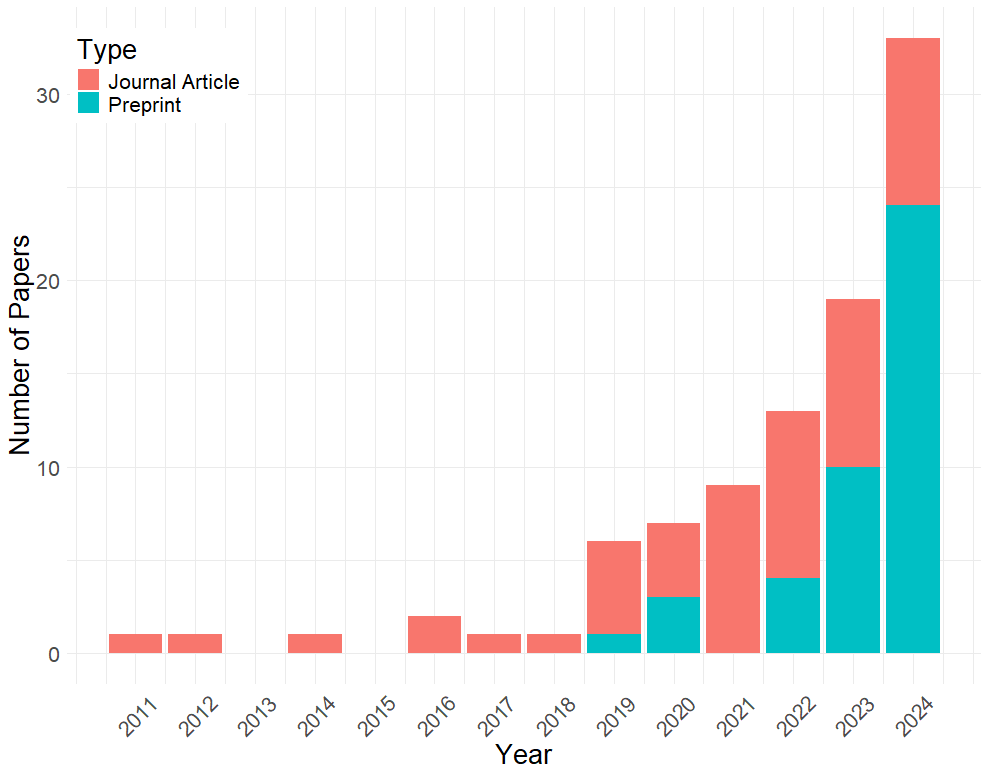
Figure 1: Trends in research output on the intersection of causal inference, machine learning, and earth observation.

Thematically, the majority of papers collected through the search query focused on environmental or earth sciences, and/or methods development of causal discovery and estimation (see §8.1 for details). Preprints tend to outnumber journal articles in recent years. This signals that the cross-fertilization between the geography of poverty and causal ML research is in the early stages. There was only a small number of substantive published papers focusing on poverty or other social science topics. This indicates that while the methodological foundations for ML-based causal inference with EO data are being forged, substantive poverty research is only now starting to integrate this perspective.

Table 1 summarizes a sampling of papers of greatest relevance to the CI-EO-ML analysis of poverty found in this search. Although we will cover themes from this table in turn in the review, we observe that, so far, the geographic reach of the predictive EO-ML work has been more expansive than the causal EO-ML literature (which has primarily focused on country-level effects). This focus indicates space for expanding the reach of causal EO-ML work to the planetary scale. We also find that the majority of papers in the causal space use EO data for outcome imputation, as opposed for deconfounding or heterogeneity decomposition.

Table 1: Summary of papers in the EO-ML poverty and poverty-adjacent literature.

Reference	EO Use	EO Data Type	Context	Estimation
–Predictive EO-ML–
[22]	Estimate electrification	Nightlight	Sub-Saharan Africa	Structural
[33]	Estimate poverty	Daylight	Africa	CNN
[58]	Estimate incomes	Daylight	Global	Random projections
[51]	Estimate poverty	Temporal multi-spectral, nightlight	Africa	CNN + RNN
–Causal EO-ML–
[55]	Impute livelihood outcomes in causal analysis	Dalight, multi-temporal	Uganda	CNN, difference-in-differences
[46]	Estimate DAG	Daylight	Simulated	SEM
[27]	Impute vehicle traffic outcomes in causal analysis	Daytime, multi-temporal	Philippines	CNN, difference-in-differences
[64]	Impute housing change outcomes in causal analysis	Daytime multi-temporal	Mongolia	CNN, stacked Granger causality
[34]	Estimate CATEs (cash transfer treatment)	Multispectral (ETM+)	Uganda	Bayesian CNN, heterogeneity model
[35]	Deconfound aid effectiveness	Multispectral (ETM+)	Nigeria	CNN, random projections with IPW

3 Spatial Statistical Approaches Towards the Geography of Poverty Without EO Data

This growth in work at the intersection of EO, ML, and causality in the study of poverty derives from earlier literature on welfare stemming from the early days of social science and evolving to the current day. In order to provide context for the EO-ML-causality intersection described later, we summarize some of these early developments here, discussing the implications of previous advancements in GIS computation, local data availability, and how spatial effects have been traditionally modeled. While this is not a complete history of the geography of poverty, details provided herein will motivate our later recommendations for the EO-ML-causal intersection.

The study of poverty—the flip side of economic prosperity—has, of course, deep roots. While some early work focused on the description of relative deprivation from a class struggle perspective [43], a shift occurred in the 1970s where the quantification of relative welfare became a focal point [66]. In the decades to follow, the rise of the welfare state and the growth in economic inequality globally prompted attention to poverty’s social and geographical elaboration [3]. Scholarship clarified “people poverty”—where poverty clustered among specific groups—and “place poverty”’—where specific structural issues tied to a geographical location could compound disadvantages [52]. While earlier poverty research was directed towards inner cities where the most acute deprivation was observed in the European or US contexts, some scholars pointed to a growing need to widen the scope to urban, suburban, and rural poverty at a global scale [44].

The 1990s also heralded an age of improvements in mapping technologies and computation acknowledged as motivating factors in propelling the geography of poverty forward. Previously, poverty and inequality were often calculated as national or regional statistics. These large areas of aggregation can obfuscate the phenomena unfolding at finer resolutions at the city, neighborhood, block, and household levels (see the discussion in, e.g., [7]). Poverty maps were then created from the desire to study the ways in which inequality varies across finer resolution, motivating new avenues in the study of the geography of poverty [44]. These large-scale poverty maps were made possible in the mid-1990s due to advancements in GIS technologies and the growing availability of geocoded local data such as the US Census Bureau’s Topologically Integrated Geographic Encoding and Referencing (TIGER) [69]. In this way, some of the earliest work quantifying poverty at refined spatial scales was centered on wealthy countries with high state capacity and well-financed census administrations.

During this process of elaborating poverty’s spatial dynamics, economists were producing various metrics to measure poverty at neighborhood levels. For some, poverty, commonly understood as economic disadvantage, shifted towards a multifaceted understanding that incorporates broader aspects of human living conditions. The capability poverty theory proposed by [63] greatly influenced subsequent measurement scholars, transforming how poverty is studied and understood. While the definition of poverty has expanded and many scholars agree with the new standards, a major theme in the geography of poverty literature lies in the continued dominance of economic indicator operationalizations [52]. For example, the [6] used a consumption-based poverty line, such as the $1 a day threshold. Another common quantitative measure is the international wealth index (IWI), an asset-based approach created from ownership of features such as consumer durables and housing characteristics from available surveys. Reasons for this continued income focus largely stem from the ability to make international comparisons with such measures. Still, there are alternative measures such as the human development index (HDI) [54] and multidimensional poverty index (MPI) [53] based on health, education, and living standards where the HDI is calculated at aggregated levels and the MPI with micro-data (e.g., individual-level credit or household survey data).

Such quantifications of poverty led to the documentation of spatial poverty traps (SPT) defined as the agglomeration and persistence of poverty in specific regions [32]. While SPTs are locally clustered, researchers have recognized SPTs in numerous countries across the world; SPTs are not a unique feature to specific regions or nations. Theorists have posited that SPTs form in response to the lack of geographical capital [8], fragile ecological environment [71], and political disadvantages [15] as their causes. While most scholars believe there are strong geographic elements that are tied to agricultural productivity, related to climate as well as the spread of diseases [62], recent arguments are less spatial and focused on institutional factors [1] as main drivers of reinforcing or liberating spatial poverty traps.

To quantify SPTs and other spatial phenomenon, various spatial models were developed. For example, one such model, spatial autocorrelation, which differs from traditional correlation as it pertains to within-variable relationships across georeferenced space. Before 1968, terms like “spatial dependence,” “spatial association”, “spatial interaction”, and “spatial interdependence” were used [25], with “spatial autocorrelation” eventually becoming the term of choice. When the spatial distribution of the outcomes is not randomly distributed across space, regression models can be misspecified as they are missing key explanatory information containing spatial dependence [39].

In models developed to capture such spatial dependence, the outcome for one observation, $Y_{i}$, would be present in the outcome model of another observation, $Y_{j}$. For example, if we sought to predict poverty levels in village $i$ in year $t$, a traditional regression model might use poverty levels in year $t-1$. But if we incorporate spatial autoregression, poverty levels in neighboring village $j$ would also affect the prediction of poverty in village $i$ [70].

More specifically, the spatial autoregressive structure is denoted by a $n\times n$ spatial weights matrix $\mathbf{W}$, with each entry, $ij$, representing the spatial dependency between unit $i$ and $j$ (and with $W_{ii}$ usually set to 0). Here, $i$ and $j$ might represent a location/scene, such as a physical address, or may represent a geographically demarcated unit, such as the centroid of a pixel. The spatial weights matrix can take numerous forms depending on researcher conceptualizations of the process being studied; examples include contiguity, distance, and nearest-neighbor elaborations [28]. See Appendix 8.2 for details.

In summary, the geography of poverty has been bolstered by the work of several domains and has continued to evolve over its inception. New technologies, data, and models have shaped the conception of poverty—how spatial poverty traps can be mapped and identified. While the past four decades have steadily grown the field via spatial models involving an assumed functional form of distance-defined spatial dependencies, in the next section, we discuss recent trends that include more flexible modeling approaches for the prediction of poverty using machine learning.

4 Machine Learning Approaches Towards the Geography of Poverty With EO Data

To address some of the aforementioned limitations of traditional statistical methods, in particular, the restricted functional form of the spatial dependence, and to leverage rapid progress in computer vision, a number of machine learning methods have been developed to process earth observation data streams (we denote this strand of literature as EO-ML). The theme here is that spatial information, previously modeled as distance alone, can be further unpacked by examining specific factors in the built environment visually captured in satellite imagery.

Grid-cell poverty prediction is perhaps the most prominent use of ML methods in the geography of poverty. Whereas sub-national poverty maps discussed in §3 have primarily been collected by governments at an administrative unit of analysis (e.g., ADM2 level), EO-ML has contributed to the creation of higher-resolution maps. This use of satellite images also allows for the imputation of missing poverty data, where missingness is present due to civil conflict or resource constraints on survey sampling.

In EO-ML poverty prediction, analysis takes the following form:

$$\widehat{\mathbb{E}}\left[Y_{i}\,\mid\,\mathbf{M}_{i}=\mathbf{m}\right]=f_{\bm{\theta}}(\mathbf{m}),$$

where $Y_{i}$ denotes the poverty outcome in question, $f_{\bm{\theta}}$ denotes a machine learning model defined with parameters $\bm{\theta}$ and $\mathbf{M}_{i}$ denotes EO image arrays. In other words, we use the EO image data to form predictions of poverty in different grid cells indexed by $i$ (where grid cells can be as precise as 1 km by 1 km). Effort has evolved from the use of nightlight-only images [21, 22], to joined night-light and daytime images [33], to night-light, daytime, and supplementary non-EO (but still spatially-resolved) datastreams [42]. Whereas the spatial statistics literature generally modeled outcomes assuming interdependence between spatial units proportional to distance between them, here, the associations between different spatial locations in the image arrays are allowed to flexibly interact with all other locations via convolutional or attention-based modeling strategies (with the former modeling spatial interactions generically as correlations of spatial locations in the image with target patterns (termed filters) and the latter modeling spatial interdependencies as weighting edges between pixels in an implicit network representation of the image).

Some of these EO-ML applications use transfer learning methods in $f_{\bm{\theta}}$, where computer vision models using CNN or ViT backbones built for one purpose are adapted for the prediction of poverty. For example, [45] leverage transfer learning approaches, using pre-trained deep learning models (VGG-Net, Inception-Net, ResNet, and DenseNet) to extract features from daytime satellite imagery, which are then used as inputs in a LASSO regression model to predict poverty levels. In a related approach, [58] use randomized feature mappings between the image and vector representations, followed by a predictive ridge regression step, to avoid the need to fall back on computationally expensive transfer learning models trained for a different purpose while still yielding performant models.

To supplement these traditional machine learning approaches where labeled poverty data (e.g., from DHS surveys) are used to form poverty predictions with EO data, there is also now a rapidly growing set of earth-observation-based foundation models for generating representations of image data that can be used in downstream poverty prediction tasks [68, 24]. In contrast to the supervised approach, EO foundation model methods often use self-supervised techniques wherein patches of input satellite images are randomly masked (i.e., held out); the rest of the image is then fed through a vision model (e.g., ViTs) to predict the masked image portion [5]. A benefit of using EO foundation models for poverty analysis is that predictions of poverty based on image information from one location can be improved by leveraging large amounts of image data from outside the study area, as these foundation models are trained on terabytes of global image information.

At the same time that EO-ML researchers interested in poverty may turn to foundation models, researchers are now starting to leverage the temporal aspect of satellite imagery. EO data streams contain temporal slices on a weekly (e.g., in Landsat images) to daily (e.g., in Maxar commercial images) basis, allowing for complex patterns of development and changes to the built environment to be modeled in generating a latent understanding of the kind of place under consideration. By incorporating temporal dependence in models, a higher degree of accuracy can be achieved, as illustrated in [51]. An implication of this work is that satellite time sequences reveal information about the progression of economic development, enabling improved predictions about the level of development at any given time slice.

There are several important considerations to be made when performing EO-ML analysis in a spatially sensitive way. First, in a comparison of various ML methods against ordinary least squared regression, the neural nets performed slightly better on prediction and reducing spatial autocorrelation of residuals [67], that is, the systematic mis-prediction of outcomes in a spatially clustered way. CNNs were not included, but non-linear models seemed to perform better overall. Still, research needs to be conducted to understand where residual spatial autocorrelation proliferates, and whether this is due to data or model. To explore this question further, there are techniques like blocked cross-validation which can deal with different interactions among the units of interest such as temporal, spatial, group, and phylogenetic/hierarchical structure [57] to test for dependence structures and yield more realistic assessments of out-of-sample performance.

In addition to spatial residual correlations in the EO-ML model pipeline, a second consideration for substantive work relates to the choice of EO image representation, which can substantially affect downstream conclusions regarding neighborhood poverty prediction. For example, while foundation models are promising in that they are specifically trained using a large corpus of satellite images (unlike random projection and many transfer learning approaches), they are not only expensive to train [65], but also not specifically tuned to capture socio-economic dynamics. Transfer learning approaches are constrained by how the data used to train the original model are often photographs (not satellite data), limiting their predictive power. In addition, randomized image representations are computationally efficient and do not require the fitting of complex models, but they are also limited in their ability to represent intricate associations between images and, e.g., spatial poverty outcomes. In this way, there are a number of tradeoffs in the EO-ML prediction of poverty that researchers must grapple with in applied work.

Integration of spatially resolved non-EO data. While EO data has lent a new perspective for understanding spatially resolved levels of development, the rise in flexible ML methods has led to use of data to supplement EO sources in poverty quantification. For instance, Google search trends can offer near real-time indicators for economic activity [17], while poor areas, which usually correlate with “data poor” regions, can be measured with mobile phone call record details [11]. These data can provide insights into population mobility, social connectedness, and communication patterns, which may be indicative of economic status. However, the use of mobile and network data raises concerns about privacy, representativeness, and potential biases. Not everyone has equal access to mobile phones or social media, and usage patterns may differ across socio-economic groups [40].

Furthermore, the availability and quality of these alternative data sources can vary significantly across countries and regions. Nationally representative surveys, such as the Demographic and Health Surveys (DHS) and the Living Standards Measurement Study (LSMS), remain important for providing consistent and reliable data on poverty and related indicators. These surveys are designed to be representative at the national and sub-national levels, allowing for comparisons across different geographic areas and population subgroups and forming the training data for EO-ML models.

In summary, while EO-based poverty predictions show potential, integrating multiple data sources, including census data, mobile phone data, and nationally representative surveys, can provide a more comprehensive understanding of poverty.

5 Causal Machine Learning With EO Data

While the integration of EO and ML methods in the geography of poverty has shown promise in predicting poverty outcomes in ways that leverage the information content of the built environment captured via image arrays, a third major strand of research has recently emerged that aims to synthesize causal inference, machine learning, and spatial analysis. In this emerging strand of research, visual signals of the built environment are still leveraged beyond spatial distance alone—not just to predict outcomes, but also now to generate counterfactuals for improving policy understanding and action. In this section, we discuss four distinct ways in which EO data, together with ML methods, can be incorporated into the causal analysis of poverty—(1.) poverty outcome imputation for downstream causal analysis, (2.) EO image deconfounding, (3.) EO-based treatment effect heterogeneity, and (4.) EO-based transportability analysis.

By way of introduction here, we note that, although this causal EO-ML literature is growing, much initial work on the intersection of EO-ML and CI-ML has been conducted in the earth and environmental sciences realm [60, 49]. This early work on causal inference with EO data was conducted in the natural sciences since there are physical laws relating radiance (e.g., Watts per square meter per steradian measured in satellite images) with physical processes on the ground (for an early example, see the discussion of how leaf temperature has been inferred from satellite data [10]). The social sciences have fewer, if any, such governing laws relating radiance from satellite data with economic processes. Therefore, there has been a greater reliance on inductive machine-learning methods.

Motivation for this evolution seems to be at least twofold. First, while [13] contrasts the model-based and algorithmic ideologies to statistical modeling and the need to move past exclusive dependence on generalized linear models in the analysis of socio-economic systems, a third culture is also proposed for the need to embrace a hybrid modeling culture that incorporates the deductive and inductive features from the data [18]. Rather than only obtaining predictions of poverty from data, there is thus interest in probing cause-effect mechanisms through a CI-ML lens. In this context, a quantity of interest is the discovery of the latent Directed Acyclic Graph relating the various structures present in the image with one another causally, among other quantities we will explore later.

Relatedly, there is also a movement to move beyond linear models in the analysis of causal inference in the spatial setting. This movement is not without potential limitations. For example, [48] observes three obstacles for CI-ML: adaptability to new circumstances, lack of explainability, and lack of native cause-effect comprehension of ML systems. Despite this, ML can support causal inference by finding more accurate statistical functionals relating outcomes, exposures, and covariates while allowing for the decomposition of treatment effect responses [37].

Poverty outcome imputation for downstream causal analysis. With this motivation in mind, we observe that scholars investigating the causes of poverty with EO data have, as an initial entry, used ideas from the previous section on satellite-based predictions of poverty with causal inference methods. For example, [55] measured the impacts of electrification in Uganda by combining EO-ML predictions of local livelihood measures in difference-in-differences (DiD) analyses. Another study combined EO-ML classification and enumeration of automobiles with DiD to measure change in traffic volumes following construction of a new airport [27]. Here, the logic of using EO data to predict outcomes found in §4 is directly applied to the causal inference context while using long-standing identification practices such as DiD.

EO-based deconfounding. There is also interest in using satellite imagery to analyze causal effects underlying the geography of poverty in observational data. For example, [23] use causal discovery algorithms to propose relationships in satellite-based representations of spatial systems which can be used to distinguish correlation from causation.

Moreover, EO data can also be used in a related way in order to model the spatial factors that led to non-experimental interventions such as the allocation of aid [35]. That is, there are a number of factors why some places, but not others, receive interventions such as aid. Techniques, such as geographic regression discontinuity, attempt to remove the influence of such spatially resolved factors by comparing places close to each other, one of which receives, the other of which does not receive the intervention [29]. While this design can be useful, spillovers and other factors complicate analysis. In an alternative design, satellite imagery, which contains information about a host of economic, geographic, and environmental factors, can potentially proxy for some of the unobserved reasons why interventions are placed where they are in order to deconfound analyses by modeling the probability of the intervention, given the image:

$$\widehat{\Pr}(W_{i}\mid\mathbf{M}_{i}=\mathbf{m})=\tilde{f}_{\bm{\theta}}(\mathbf{m}),$$

where, again, $\tilde{f}_{\bm{\theta}}(\cdot)$ defines a machine learning model with parameters $\bm{\theta}$ relating the image or image sequence information, $\mathbf{M}_{i}$ with the probability of treatment. This probability can then be used in double machine learning or inverse probability weighting methods [38].

EO-based treatment effect heterogeneity. While EO data are useful in estimating effects of anti-poverty interventions on an observational basis using ML methods, CI-EO-ML literature has also begun using EO data in the analysis of treatment effects in experimental data. For example, [34] estimate conditional average treatment effects (CATEs) using satellite data to model the kinds of neighborhoods most responsive to anti-poverty interventions. In this literature, there is substantive and policy interest in modeling

$$\textrm{CATE}(\mathbf{m})=\mathbb{E}[Y_{i}(1)-Y_{i}(0)\mid\mathbf{M}_{i}=\mathbf{m}],$$

where $\mathbf{M}_{i}$ represents a satellite image or image sequence representation around $\mathbf{M}_{i}$’s location (where $i$ could be a household or a village) and where $Y_{i}(1)-Y_{i}(0)$ represents the different in poverty outcomes with and without an economic intervention (such as a cash transfer). Substantively, $\textrm{CATE}(\mathbf{m})$ can inform decision-makers about the kinds of neighborhood structures where individuals are most responsive to anti-poverty interventions.

EO-based effect transportability. The model for $\textrm{CATE}(\mathbf{m})$’s can also be applied, with or without re-weighting, to the area outside the original geographic context of the experiment, as image data is available not only for experimental sites but also all others in a region of interest, expanding the reach of transportability analysis [20]. This sort of dis-aggregation can help identify individuals or groups harmed by an overall effective treatment for the development of policy optimization rules [61]. EO foundation models, randomized projections, and end-to-end ML architectures can also be used in translating the raw image array, $\mathbf{M}_{i}$, into a useful representation for heterogeneity decomposition.

In short, causal inference methods have been advanced to handle EO image arrays to model cause and effect as it relates to neighborhood-level poverty. Some of this work has focused on using EO-ML imputed poverty outcomes in causal analyses; others have used EO data for treatment effect heterogeneity reasoning or for deconfounding.

6 Discussion & Future Directions

This review has analyzed the evolution of the geography of poverty. In §3, we explored traditional spatial statistical methods used with government or researcher-collected data to explore poverty at the individual and group levels. We argued that spatial statistical methods, while valuable in contributing to clear deductive research questions, have limits in the expressivity of non-linear relationships and complex data structures.

We then discussed the rise of machine learning methods paired with EO data to address the limitations of strongly parametric models with researcher-defined spatiotemporal interdependencies. This area has seen rapid growth in the prediction of poverty [33], the study of spatial interdependencies in poverty prediction using machine learning and Earth observation data, and in the integration of non-EO data sources such as mobile phone data and social network data to improve poverty estimates [12]. EO-ML opened up new opportunities in the field, with models that were more accurate and generalizable than traditional methods. Lastly, we analyzed the work of causal ML and its promise of a hybrid modeling culture that combines causal reasoning with AI in the geography of poverty. Figure 2 summarizes some of the choices involved in causal EO-ML workflows.

Figure 2: EO-ML causal workflow.

1. Define research question, measurement strategy, and causal quantity of interest

   • Determine role of EO data

     • Outcome imputation: Image as observed outcome predictor? ATE or CATE estimand

     • Observational inference: Image deconfounder? ATE estimand

     • Experimental inference: Image heterogeneity? CATE estimand

   • Clarify poverty measures (e.g. asset-based poverty index, consumption)

   • Identify potential treatment/exposure variables (e.g., aid, economic intervention)

   • Consider relevant spatial/temporal scales (e.g., yearly, quarterly)

2. Collect and preprocess EO & non-EO data

   • Acquire outcome or poverty data from surveys (e.g., DHS), censuses, experiments

   • Obtain relevant EO data (e.g., satellite imagery, night lights, etc.)

   • Obtain relevant non-EO data (e.g., cell phone coverage)

3. EO-ML-CI Identification strategy

   • Assess plausibility of identifying assumptions given data and causal model; perform balance tests

4. Estimation strategy

   • Choose ML models for nuisance parameters (e.g. propensity scores, outcome models)

     • Consider randomized projection models for image representations

     • Consider EO foundation models for image representations

     • Consider pre-trained image foundation models for image representations

     • Consider models that leverage spatial and temporal structure (e.g. CNNs, RNNs, ViTs)

   • Select model hyperparameters via spatial cross-validation

5. Estimate causal effects

   • Compute point estimates and confidence intervals using bootstrap, cross-fitting, or Bayesian methods

   • Validate estimates on held-out test sets, new time periods, and/or new geographies

6. Interpret results

   • Examine gradient/salience maps

   • Observational inference: Examine highest/lowest treatment probability images

   • Experimental inference: Examine highest/lowest responder images

   • Analyze transportability by applying causal model to more expansive geographic area

Open questions remain regarding how to handle spatial interdependencies in the EO-ML causal framework, which has primarily made various assumptions about scenes (e.g., villages depicted in satellite image arrays) being independent. This assumption might not be satisfied in some cases, violating a fundamental assumption of causal inference known as the stable unit treatment value assumption (SUTVA) [59]. SUTVA assumes that units are independent with no interactions amongst other observations and that there is a single version of the treatment. Spatial dependence and some forms of economic interaction break these assumptions because proximity effects occur between units, and spatial variation can lead to different versions of treatments [2]. While some methods, such as the block bootstrap, can be used in causal machine-learning pipelines to handle spatial dependencies, there is still room to develop best practices, especially given the presence of spatial interdependencies possible in treatment, pre-treatment covariates, mediators, and outcomes [2].

Future work should also examine privacy and fairness issues with causal analyses based on passive sensor technologies. For example, even if an analysis using EO data does not explicitly contain information about some variable, such as race, not for inclusion in the analysis products for legal or ethical reasons, such information may nonetheless be imprinted in the built environment. Thus, the EO data streams may have statistical associations with the forbidden variable requiring further processing (e.g., [56]). This consideration could also motivate the use of synthetic EO or population data streams [72].

Third, there are a host of open questions at the intersection of EO-ML-based causal inference and EO foundation models. While foundation models may generate useful representations of EO data streams for causal heterogeneity or confounding analysis, foundation model weights contain information from the entire training period of images (usually both pre- and post-treatment, especially for historical interventions). Therefore, use of EO-ML foundation models in causal inference may face a problem of treatment leakage [19], where treatment information may be found in pre-treatment representations of the target image set.

7 Conclusion

In this chapter, we focused on the growing field of causal ML and its implications on the geography of poverty, which led us to first investigate the small but growing body of papers, both published and pre-prints, that attempt to combine causal EO-ML methods and applications. Our investigation of this literature uncovered several open questions. We observed that some of the conversation thus far has kept spatial considerations implicit in the analysis, with an underexplored distinction between EO data and spatial dynamics. Indeed, the relationship between the spatial information contained in satellite data streams and spatial dynamics traditionally understood in statistical models is still being clarified; there is space for human geographers and social scientists to form interdisciplinary research standards in this area.

Going forward, by leveraging the power of machine learning, causal inference methods, and EO data, researchers will be better equipped to unravel the web of factors contributing to poverty and to develop more effective strategies for alleviating it. This new view of the geography of poverty is grounded in existing high-quality data sources from experimenters and governments. It also develops insights from new data streams, holding promise to advance our understanding of global inequality in pursuit of a more prosperous world. $\square$

8 Appendix

8.1 A Quantitative Literature Survey

We here discuss how the papers found via SCOPUS were analyzed. The search terms used were: ‘( ‘eo’ OR ‘Earth Observation’ OR ‘satellite image*’ OR ‘remote sensing’ OR ‘earth science’ OR ‘earth’s system’ OR ‘environmental eco*’ OR ‘environmental science*’ OR ‘geosci*’) AND (‘machine learning’ OR ‘ml’ OR ‘ai’ OR ‘deep learning’ ) AND ( ‘causal inf*’ OR ‘causal relation*’ OR ‘causality’ OR ‘causal learning’ OR ‘causal effect*’ OR ‘policy eval*’ OR ‘causal impact’ OR ‘causal discovery’ OR ‘treatment effect*’ OR ‘causal representation’)”. We limited the scope of the survey to between 2011 and 2024 (as few papers appear before 2011). This resulted in 46 papers and 24 preprints.

We analyzed the SCOPUS articles and pre-prints in the following way. First, bigrams from the abstracts were analyzed; Table Table 2 shows bigrams that appeared over 8 times. Beyond the expected results, some of the notable bigrams are time series, which occurred 25 times, earth system/ sciences 18 and 11, and causal discovery at 17 times. There are some trends in the type of data being processed, like time series or remotely sensed variety, the domains being studied, like earth sciences, and the types of methods or concepts, like causal discovery and Granger causality, that repeatedly show up in the nascent literature.

	Abstract Bigram	Count
1	machine learning	45
2	remote sensing	31
3	causal inference	30
4	deep learning	27
5	time series	25
6	earth system	18
7	causal discovery	17
8	causal relationships	13
9	earth sciences	11
10	neural network	11
11	granger causality	10
12	building damage	9
13	causal effects	8
14	crop diversification	8
15	feature extraction	8
16	satellite imagery	8
17	spurious variables	8

Table 2: Top bigrams among papers found in the literature search.

We then evaluate where papers are being published, Table 3 shows the various journal themes, with remote sensing journals having the greatest number followed by earth and environment, and then by AI/ML/CV publications. This goes to show that technologically minded journals have been utilized, followed by earth and environmental science related ones. Next, the content of the paper was evaluated by themes, and surprisingly, most of the papers were grounded in earth and environmental sciences, while only 21 of the papers focused only on technical topics. For the geography of poverty, we find that there are few papers dealing with economic topics, being far eclipsed by natural science topics.

Another finding is that technical development is being outpaced by applications. The majority of papers focus on using machine learning and causal inference methods to study substantive questions in earth and environmental sciences. Comparatively, fewer papers are solely dedicated to extending or developing novel methodologies at the intersection of these fields. This suggests there may be opportunities for more dedicated technical and methodological research to expand the toolkit for applying ML and causal inference to geospatial data.

	Journal Theme	Count
1	remote sensing	18
2	earth and environment	14
3	AI ML CV	10
4	economics	3
5	public health	1

Table 3: Journal themes in quantitative review of EO-ML literature.

In the literature found, four papers used double machine learning, five chose Granger causality, and nine used some network or graphical approach. Many of the outcomes were focused on environmental factors like vegetation, atmospheric measurements, or hydrological features. Only 12 papers were focused on socio-economic outcomes such as IWI, local development from infrastructure projects like roads, airports, and the electric grid.

	Paper Theme	Count
1	earth and environment	41
2	AI ML CV	21
3	economics	9
4	public health	1

Table 4: Paper themes in quantitative review of EO-ML literature.

Taken together, this review suggests that research at the intersection of causal inference, machine learning, and earth observation is a rapidly growing but still nascent field.

8.2 Spatial Models

The spatially-lagged outcome model has a spatial lag of the predictor variable; from the previous example, this would equate to neighboring housing prices being included in the regression for the price of a specific house. The multiplication of $\mathbf{W}$ represents a linear combination of the values of the target and neighboring values, which captures the spatial dependence through a spatially weighted average of its neighbor’s values. In its generic form, we have:

$$Y_{i}=\alpha+\rho\sum_{j=1}^{n}W_{ij}Y_{j}+\epsilon_{i},\quad i=1,\ldots,n$$

where

• $W_{ij}$ is the $ij$-th element of $\mathbf{W}$;

• $\sum_{j=1}^{n}W_{ij}Y_{j}$ is the spatially weighted average of the dependent variable;

• $\rho$ is the spatial autoregressive parameter which measures the intensity of the spatial interdependence ($\rho>0$ indicates positive spatial dependence, $\rho<0$ indicates negative spatial dependence, and $\rho=0$ indicates a traditional univariate OLS model with no dependence);

• $\epsilon_{i}$ is the error term representing unmodeled factors affecting the outcome.

Work attempting to quantify associations between various proposed causal factors and spatially-defined poverty outcomes widely adopted this sort of methodological framework to account for spatial dynamics in geographical poverty analysis [50].

References

- [1] Daron Acemoglu and James A. Robinson “Why is Africa Poor?” In Economic History of Developing Regions 25.1 Taylor & Francis, 2010, pp. 21–50
- [2] Kamal Akbari, Stephan Winter and Martin Tomko “Spatial Causality: A Systematic Review on Spatial Causal Inference” In Geographical Analysis 55.1 Wiley Online Library, 2023, pp. 56–89
- [3] Peter Alcock “Understanding Poverty.” Palgrave Macmillan, 2006
- [4] Susan Athey “The impact of machine learning on economics” In The economics of artificial intelligence: An agenda, 2018, pp. 507–547
- [5] Vijay Badrinarayanan, Alex Kendall and Roberto Cipolla “Segnet: A Deep Convolutional Encoder-decoder Architecture for Image Segmentation” In IEEE Transactions on Pattern Analysis and Machine Intelligence 39.12 IEEE, 2017, pp. 2481–2495
- [6] World Bank “World Development Report 1990: Poverty” The World Bank, 1990
- [7] Tara Bedi, Aline Coudouel and Kenneth Simler “More Than a Pretty Picture: Using Poverty Maps to Design Better Policies and Interventions” World Bank Publications, 2007
- [8] Kate Bird “Addressing Spatial Poverty Traps” In Chronic Poverty Advisory Network, London 2, 2019
- [9] Kate Bird, Kate Higgins and Dan Harris “Spatial Poverty Traps: An Overview” CPRC Working Paper 161, 2010 URL: http://cdn-odi-production.s3.amazonaws.com/media/documents/5514.pdf
- [10] Blaine L. Blad and Norman J. Rosenberg “Measurement of Crop Temperature by Leaf Thermocouple, Infrared Thermometry and Remotely Sensed Thermal Imagery” In Agronomy Journal 68.4 Wiley Online Library, 1976, pp. 635–641
- [11] Joshua E. Blumenstock “Fighting Poverty with Data” In Science 353.6301, 2016, pp. 753–754 DOI: 10.1126/science.aah5217
- [12] Joshua E. Blumenstock, Gabriel Cadamuro and Robert On “Predicting Poverty and Wealth from Mobile Phone Metadata” In Science 350.6264 American Association for the Advancement of Science, 2015, pp. 1073–1076
- [13] Leo Breiman “Statistical Modeling: The Two Cultures” In Statistical Science 16.3 Institute of Mathematical Statistics, 2001, pp. 199–231
- [14] Ryan C Briggs “Poor Targeting: A Gridded Spatial Analysis of the Degree to which Aid Reaches the Poor in Africa” In World Development 103 Elsevier, 2018, pp. 133–148
- [15] William J. Burke and Thomas S. Jayne “Spatial Disadvantages or Spatial Poverty Traps: Household Evidence from Rural Kenya” In RePEc, 2008
- [16] Raj Chetty, Nathaniel Hendren, Patrick Kline and Emmanuel Saez “Where is the Land of Opportunity? The Geography of Intergenerational Mobility in the United States” In The Quarterly Journal of Economics 129.4 MIT Press, 2014, pp. 1553–1623
- [17] Hyunyoung Choi and Hal Varian “Predicting the Present with Google Trends” In Economic record 88 Wiley Online Library, 2012, pp. 2–9
- [18] Adel Daoud and Devdatt Dubhashi “Statistical Modeling: The Three Cultures” In arXiv preprint arXiv:2012.04570, 2020
- [19] Adel Daoud, Connor T. Jerzak and Richard Johansson “Conceptualizing Treatment Leakage in Text-based Causal Inference” In Proceedings of the 2022 Conference of the North American Chapter of the Association for Computational Linguistics: Human Language Technologies Seattle, United States: Association for Computational Linguistics, 2022, pp. 5638–5645 DOI: 10.18653/v1/2022.naacl-main.413
- [20] Irina Degtiar and Sherri Rose “A Review of Generalizability and Transportability” In Annual Review of Statistics and Its Application 10 Annual Reviews, 2023, pp. 501–524
- [21] Christopher NH Doll “Estimating Non-population Ativities from Night-time Satellite Imagery” In Remotely-Sensed Cities CRC Press, 2003, pp. 335
- [22] Christopher NH Doll and Shonali Pachauri “Estimating Rural Populations Without Access to Electricity in Developing Countries through Night-time Light Satellite Imagery” In Energy policy 38.10 Elsevier, 2010, pp. 5661–5670
- [23] Imme Ebert-Uphoff and Yi Deng “Causal Discovery for Climate Research Using Graphical Models” In Journal of Climate 25.17 American Meteorological Society, 2012, pp. 5648–5665
- [24] Clay Foundation “GitHub Model Repository” Accessed: 2023-05-01, https://github.com/Clay-foundation/model, 2023
- [25] Arthur Getis “A History of the Concept of Spatial Autocorrelation: A Geographer’s Perspective” In Geographical Analysis 40.3 Wiley Online Library, 2008, pp. 297–309
- [26] Edward Glaeser “Cities, Productivity, and Quality of Life” In Science 333.6042 American Association for the Advancement of Science, 2011, pp. 592–594
- [27] Eugenia Go, Kentaro Nakajima, Yasuyuki Sawada and Kiyoshi Taniguchi “On the Use of Satellite-Based Vehicle Flows Data to Assess Local Economic Activity: The Case of Philippine Cities”, 2022 DOI: 10.2139/ssrn.4057690
- [28] Daniel A Griffith “Some Guidelines for Specifying the Geographic Weights Matrix Contained in Spatial Statistical Models” In Practical handbook of spatial statistics CRC press, 2020, pp. 65–82
- [29] Jinyong Hahn, Petra Todd and Wilbert Van der Klaauw “Identification and Estimation of Treatment Effects with a Regression-discontinuity Design” In Econometrica 69.1 JSTOR, 2001, pp. 201–209
- [30] Ola Hall, Francis Dompae, Ibrahim Wahab and Fred Mawunyo Dzanku “A review of machine learning and satellite imagery for poverty prediction: Implications for development research and applications” In Journal of International Development 35.7 Wiley Online Library, 2023, pp. 1753–1768
- [31] John R Hipp “General Theory of Spatial Crime Patterns” In Criminology 54.4 Wiley Online Library, 2016, pp. 653–679
- [32] Jyotsna Jalan and Martin Ravallion “Spatial Poverty Traps?” World Bank, Development Research Group Washington, DC, USA, 1997
- [33] Neal Jean et al. “Combining Satellite Imagery and Machine Learning to Predict Poverty” In Science 353.6301 American Association for the Advancement of Science, 2016, pp. 790–794
- [34] Connor T. Jerzak, Fredrik Johansson and Adel Daoud “Image-based Treatment Effect Heterogeneity” In Proceedings of the Second Conference on Causal Learning and Reasoning (CLeaR), Proceedings of Machine Learning Research (PMLR) 213, 2023, pp. 531–552
- [35] Connor T. Jerzak, Fredrik Johansson and Adel Daoud “Integrating Earth Observation Data into Causal Inference: Challenges and Opportunities” In arXiv preprint arXiv:2301.12985, 2023
- [36] George Em Karniadakis et al. “Physics-informed Machine Learning” In Nature Reviews Physics 3.6 Nature Publishing Group, 2021, pp. 422–440
- [37] Shiho Kino et al. “A Scoping Review on the Use of Machine Learning in Research on Social Determinants of Health: Trends and Research Prospects” In SSM-population Health 15 Elsevier, 2021, pp. 100836
- [38] Michael C Knaus “Double Machine Learning-based programme Evaluation Under Unconfoundedness” In The Econometrics Journal 25.3 Oxford University Press, 2022, pp. 602–627
- [39] Yingji Li et al. “Mitigating Social Biases of Pre-trained Language Models via Contrastive Self-Debiasing with Double Data Augmentation” In Artificial Intelligence Elsevier, 2024, pp. 104143
- [40] Alejandro Llorente, Manuel Garcia-Herranz, Manuel Cebrian and Esteban Moro “Social Media Fingerprints of Unemployment” In PloS one 10.5 Public Library of Science San Francisco, CA USA, 2015, pp. e0128692
- [41] Linda M Lobao, Gregory Hooks and Ann R Tickamyer “The Sociology of Spatial Inequality” Suny Press, 2007
- [42] Robert Marty and Alice Duhaut “Global Poverty Estimation using Private and Public Sector Big Data Sources” In Scientific Reports 14.1 Nature Publishing Group UK London, 2024, pp. 3160
- [43] Karl Marx “Karl Marx: Selected Writings” Oxford University Press, USA, 2000
- [44] Paul Milbourne “The Geographies of Poverty and Welfare” In Geography Compass 4.2 Wiley Online Library, 2010, pp. 158–171
- [45] Ye Ni et al. “An Investigation on Deep Learning Approaches to Cmbining Nighttime and Daytime Satellite Imagery for Poverty Prediction” In IEEE Geoscience and Remote Sensing Letters 18.9 IEEE, 2020, pp. 1545–1549
- [46] Soronzonbold Otgonbaatar, Mihai Datcu and Begüm Demir “Causality for Remote Sensing: An Exploratory Study” ISSN: 2153-7003 In IGARSS 2022 - 2022 IEEE International Geoscience and Remote Sensing Symposium, 2022, pp. 259–262 DOI: 10.1109/IGARSS46834.2022.9883060
- [47] Georgia Papadogeorgou, Kosuke Imai, Jason Lyall and Fan Li “Causal Inference with Spatio-temporal Data: Estimating the Effects of Airstrikes on Insurgent Violence in Iraq” In Journal of the Royal Statistical Society Series B: Statistical Methodology 84.5 Oxford University Press, 2022, pp. 1969–1999
- [48] Judea Pearl “The Seven Tools of Causal Inference, with Reflections on Machine Learning” In Communications of the ACM 62.3 ACM New York, NY, USA, 2019, pp. 54–60
- [49] Adrián Pérez-Suay and Gustau Camps-Valls “Causal Inference in Geoscience and Remote Sensing From Observational Data” Conference Name: IEEE Transactions on Geoscience and Remote Sensing In IEEE Transactions on Geoscience and Remote Sensing 57.3, 2019, pp. 1502–1513 DOI: 10.1109/TGRS.2018.2867002
- [50] Alessandra Petrucci, Nicola Salvati and Chiara Seghieri “The Application of a Spatial Regression Model to the Analysis and Mapping of Poverty” Food & Agriculture Org., 2003
- [51] Markus B. Pettersson et al. “Time Series of Satellite Imagery Improve Deep Learning Estimates of Neighborhood-level Poverty in Africa” In Proceedings of the Thirty-Second International Joint Conference on Artificial Intelligence, 2023, pp. 6165–6173
- [52] Martin Powell, George Boyne and Rachel Ashworth “Towards a Geography of People Poverty and Place Poverty” In Policy & Politics 29.3 Policy Press, 2001, pp. 243–258
- [53] UNDP (United Nations Development Programme “2023 Global Multidimensional Poverty Index (MPI): Unstacking Global Poverty: Data for High Impact Action” UNDP (United Nations Development Programme, 2023
- [54] UNDP (United Nations Development Programme) “Human Development Report 1990: Concept and Measurement of Human Development” UNDP (United Nations Development Programme), 1990
- [55] Nathan Ratledge et al. “Using Machine Learning to Assess the Livelihood Impact of Electricity Access” Num Pages: 23 Place: Berlin Publisher: Nature Portfolio Web of Science ID: WOS:000884842400024 In Nature 611.7936, 2022, pp. 491–+ DOI: 10.1038/s41586-022-05322-8
- [56] Shauli Ravfogel et al. “Null It Out: Guarding Protected Attributes by Iterative Nullspace Projection” In arXiv preprint arXiv:2004.07667, 2020
- [57] David R Roberts et al. “Cross-validation strategies for data with temporal, spatial, hierarchical, or phylogenetic structure” In Ecography 40.8 Wiley Online Library, 2017, pp. 913–929
- [58] Esther Rolf et al. “A Generalizable and Accessible Approach to Machine Learning with Global Satellite Imagery” In Nature Communications 12.1 Nature Publishing Group UK London, 2021, pp. 4392
- [59] Donald B Rubin “Comment: Which Ifs Have Causal Answers” In Journal of the American statistical association 81.396 Taylor & Francis, 1986, pp. 961–962
- [60] Jakob Runge et al. “Causal Inference for Time Series” Num Pages: 19 Place: London Publisher: Springernature Web of Science ID: WOS:001017712700002 In Nature Reviews Earth & Environment 4.7, 2023, pp. 487–505 DOI: 10.1038/s43017-023-00431-y
- [61] Mehak Sachdeva and A Stewart Fotheringham “A Geographical Perspective on Simpson’s Paradox” In Journal of Spatial Information Science, 2023, pp. 1–25
- [62] Jeffrey D Sachs, Andrew D Mellinger and John L Gallup “The Geography of Poverty and Wealth” In Scientific American 284.3 JSTOR, 2001, pp. 70–75
- [63] Amartya Sen “Development as Capability Expansion” In The community development reader 41, 1990, pp. 58
- [64] Batkhurel Serdavaa “A Satellite Image Analysis on Housing Conditions and the Effectiveness of the Affordable Housing Mortgage Program in Mongolia: A Deep Learning Approach”, 2023 DOI: 10.2139/ssrn.4664966
- [65] Craig Smith “What Large Models Cost You – There Is No Free AI Lunch” Accessed: 2024-05-02, 2023
- [66] David M. Smith “Human Geography” London, England: Hodder Arnold, 1977
- [67] Insang Song and Daehyun Kim “Three Common Machine Learning Algorithms Neither Enhance Prediction Accuracy Nor Reduce Spatial Autocorrelation in Residuals: An Analysis of Twenty-five Socioeconomic Data Sets” In Geographical Analysis 55.4 Wiley Online Library, 2023, pp. 585–620
- [68] Aristeidis Tsaris et al. “Pretraining Billion-scale Geospatial Foundational Models on Frontier” In arXiv preprint arXiv:2404.11706, 2024
- [69] U.S. Census Bureau “Celebrating 25 Years of TIGER”, U.S. Census Bureau, 2023 URL: https://www.census.gov/programs-surveys/geography/about/training/25-years-tiger.html
- [70] John P Wilson “Geographic Information Science & Technology: Body of Knowledge 2.0 Project” In Final Report: University Consortium for Geographic Information Science, 2014
- [71] Zhenshan Yang, Ding Yang, Dongqi Sun and Linsheng Zhong “Ecological and Social Poverty Traps: Complex Interactions Moving Toward Sustainable Development” In Sustainable Development 31.2 Wiley Online Library, 2023, pp. 853–864
- [72] Matthew Yates et al. “Evaluation of Synthetic Aerial Imagery using Unconditional Generative Adversarial Networks” In ISPRS Journal of Photogrammetry and Remote Sensing 190 Elsevier, 2022, pp. 231–251