Towards high-order consistency and convergence of conservative SPH approximations

Abstract

Smoothed particle hydrodynamics (SPH) offers distinct advantages for modeling many engineering problems, yet achieving high-order consistency in its conservative formulation remains to be addressed. While zero- and higher-order consistencies can be obtained using particle-pair differences and the kernel gradient correction (KGC) approaches, respectively, for SPH gradient approximations, their applicability for discretizing conservation laws in practical simulations is limited due to their non-conservative feature. Although the standard anti-symmetric SPH approximation is able to achieve conservative zero-order consistency through particle relaxation, its straightforward extensions with the KGC fail to satisfy either zero- or higher-order consistency. In this paper, we propose the reverse KGC (RKGC) formulation, which is conservative and able to precisely satisfy both zero- and first-order consistencies when particles are relaxed based on the KGC matrix. Extensive numerical examples show that the new formulation considerably improves the accuracy of the Lagrangian SPH method. In particular, it is able to resolve the long-standing high-dissipation issue for simulating free-surface flows. Furthermore, with fully relaxed particles, it enhances the accuracy of the Eulerian SPH method even when the ratio between the smoothing length and the particle spacing is considerably reduced. Indeed, the reverse KGC formulation holds the potential for the extension to even higher-order consistencies. However, addressing the corresponding particle relaxation problem remains a pending challenge.

1 Introduction

As a mesh-free method, smoothed particle hydrodynamics (SPH), initially proposed by Lucy [1] and Gingold & Monaghan [2] for astrophysical applications, has demonstrated significant success across a wide range of scientific problems. These include fluid dynamics [3, 4, 5], solid dynamics [6, 7, 8], and fluid-structure interaction [9, 10, 11], among others. The SPH approximation operates on the principle of reconstructing the continuous field and its spatial derivatives from a collection of discrete particles, each possessing individual properties, through a Gaussian-like smoothing kernel function with compact support [12, 13]. It generally encounters two different types of errors that amalgamate to the overall truncation error [14, 15]. The first is the smoothing error determined by the kernel function where the leading moments vanish. This error arises due to the discrepancy between the smoothing approximations and the exact values. The second is the integration error, characterized by the non-vanishing of leading moments due to the particle approximation. For typical SPH kernel functions, such as the cubic B-spline [16] and the Wendland kernel [17] are second-order accuracy, given that only the first moment vanishes, corresponding to first-order consistency. With the given kernel function, Quinlan et al. [14] observed that the overall truncation error generally decreases or exhibits consistency with increased resolution only when $h/\Delta{x}$, i.e., the ratio between the smoothing length $h$ and the particle spacing $\Delta{x}$, is large, suggesting sufficient small integration error. However, achieving this condition leads to an excessive number of particles within the kernel compact support and results in an extremely high computational cost.

Therefore, different approaches have been proposed to minimize integration error or improve consistency with a computationally acceptable value of $h/\Delta{x}$, typically less than 1.5 [18]. Besides that zero-order consistency can be easily achieved by using particle-pair differences for gradient approximations, high-order consistencies can be attained through kernel gradient correction (KGC) [19] and various similar approaches, such as corrective smoothed particle method (CSPM) [20], reproducing kernel particle method (RKPM) [21, 22], finite particle method [23], modified SPH method (MSPH) [24, 25, 26, 27], moving least squared (MLS) [28] and many others [29, 30, 31]. While these approaches are able to achieve consistencies for the SPH approximation of the gradient and/or Laplacian operators, their application to the discretization of physical conservation laws still faces a significant challenge of non-conservation. Specifically, conservative discretization necessitates an anti-symmetric form between particle pairs, a condition that these methods could not appropriately satisfy.

The first approach to achieve both zero-order consistency and conservation involves implementing the particle relaxation based on constant background pressure [15, 32] before applying anti-symmetric SPH approximations. Since the particle relaxation is computationally expensive for the Lagrangian SPH method, the alternative one-step consistency correction, such as the transport-velocity formulation [33, 34], based on the same principle, has also been proposed to enhance the consistency. Although conservation properties always hold a high priority [18], there is still an expectation for high-order consistency in SPH so that it can be utilized as a generally effective numerical method. To address this, approaches have been developed to enhance numerical accuracy and consistency by integrating KGC with anti-symmetric formulations [35, 36, 37] and/or particle relaxation [38]. These methods include utilizing the average correction matrix [39, 40, 41] and implementing separate corrections for each particle pair [18, 42], etc. For some problems, while these conservative KGC formulations have demonstrated improved results compared to standard SPH methods without KGC, as will be shown later, they not only fail to achieve high-order consistency but also lose zero-order consistency, even with particle relaxation.

In this study, we introduce the reverse KGC (RKGC) formulation designed for conservative SPH approximations. In contrast to the prior conservative KGC formulations, RKGC is able to precisely fulfill both zero- and first-order consistencies of the gradient operator. The formulation incorporates a particle relaxation driven by the KGC matrix and is distinguished into two parts: the first part addresses zero-order consistency and vanishes during particle relaxation, while the second part ensures first-order consistency and accurately reproduces the linear gradient. The formulation notably improves numerical accuracy in Lagrangian SPH simulations. In particular, it exhibits very good energy conservation properties and resolves the long-standing high-dissipation issue for the SPH simulation of free-surface flows. Moreover, since these consistencies can be strictly imposed in the Eulerian SPH method, even when employing a reduced smoothing length, the formulation still has the potential to yield results with improved accuracy.

In the following sections, Section 2 presents the approximation of gradients in the SPH method and its application in discretizing governing equations. Section 3 introduces the RKGC formulation, detailing the particle relaxation and the transport-velocity formulation based on the KGC matrix. Section 4 conducts corresponding error and convergence analyses. Following this, Section 5 presents extensive numerical examples that highlight the benefits gained from the proposed method. In Section 6, we extend the RKGC formulation to second-order consistency, with a yet-to-be-addressed condition on the particle relaxation. Finally, Section 7 summarizes the key findings and outlines of future research.

2 Preliminary

2.1 Gradient approximation

In SPH, the kernel approximation for the gradient of a smooth field $\psi\left({\boldsymbol{\rm r}}\right)$ can be expressed through a two-stage approach

$$\nabla\psi\left(\boldsymbol{\rm r}\right)\approx\int_{\Omega}\nabla\psi\left({\boldsymbol{\rm r}^{*}}\right)W\left(\boldsymbol{\rm r}-\boldsymbol{\rm r}^{*},h\right)d\boldsymbol{\rm r}^{*}=-\int_{\Omega}\psi\left({\boldsymbol{\rm r}^{*}}\right)\nabla W\left(\boldsymbol{\rm r}-\boldsymbol{\rm r}^{*},h\right)d\boldsymbol{\rm r}^{*},$$ (1)

where $W\left(\boldsymbol{\rm r},h\right)$ is the kernel function scaled by the smoothing length $h$. While the first stage introduces smoothing errors by the kernel function, the second stage entails the integration by parts, assuming the kernel function vanishes at the boundary of compact support. Through Taylor expansion, for Eq. (1), one can easily find that the zero-order consistency condition is

$$\int_{\Omega}\nabla W\left(\boldsymbol{\rm r}-\boldsymbol{\rm r}^{*},h\right)d\boldsymbol{\rm r}^{*}=0,$$ (2)

and the first-order consistency condition is

$$-\int_{\Omega}\left(\boldsymbol{\rm r}^{*}-\boldsymbol{\rm r}\right)\otimes\nabla W\left(\boldsymbol{\rm r}-\boldsymbol{\rm r}^{*},h\right)d\boldsymbol{\rm r}^{*}=\mathbf{I},$$ (3)

where $\mathbf{I}$ represents the identity matrix. Note that, with zero-order consistency condition, one can rewrite the kernel approximation in two equivalent forms:

$$\nabla\psi\left(\boldsymbol{\rm r}\right)=\int_{\Omega}\left(\psi\left({\boldsymbol{\rm r}}\right)-\psi\left({\boldsymbol{\rm r}^{*}}\right)\right)\nabla W\left(\boldsymbol{\rm r}-\boldsymbol{\rm r}^{*},h\right)d\boldsymbol{\rm r}^{*}\\ \equiv-\int_{\Omega}\left(\psi\left({\boldsymbol{\rm r}}\right)+\psi\left({\boldsymbol{\rm r}^{*}}\right)\right)\nabla W\left(\boldsymbol{\rm r}-\boldsymbol{\rm r}^{*},h\right)d\boldsymbol{\rm r}^{*}.$$ (4)

By introducing particle summation, the first approximation in Eq. (4) can be further approximated at an SPH particle $i$ as

$$\nabla\psi_{i}=\sum_{j}\psi_{ij}\nabla W_{ij}V_{j},$$ (5)

where $V_{j}$ is the volume of the neighbor particles within the support, and the particle-pair difference $\psi_{ij}=\psi_{i}-\psi_{j}$ is adopted. This form is often referred to as a symmetric or non-conservative form. Similarly, the second approximation in Eq. (4) can be further approximated as

$$\nabla\psi_{i}=-\sum_{j}\left(\psi_{i}+\psi_{j}\right)\nabla W_{ij}V_{j},$$ (6)

where the particle-pair sum is employed. This form, known as the anti-symmetric or conservative form, ensures conservation properties and is commonly chosen in classic SPH methods for the discretization of physical conservation laws.

For the non-conservative form of Eq. (5), zero-order consistency is automatically satisfied as the particle-pair difference is used. To achieve first-order consistency, one requires that the approximation of Eq. (3) satisfying

$$-\sum_{j}\boldsymbol{\rm r}_{ij}\otimes\nabla W_{ij}V_{j}=\mathbf{I}.$$ (7)

To precisely fulfill the above condition, the KGC approach [19], introducing a correction matrix $\mathbf{B}_{i}$ to adjust the gradient of the kernel function, can be employed, so that one has

$$-\sum_{j}\boldsymbol{\rm r}_{ij}\otimes\mathbf{B}_{i}\nabla W_{ij}V_{j}=\mathbf{I},\quad\mathbf{B}_{i}=\left(-\sum_{j}\mathbf{r}_{ij}\otimes\nabla W_{ij}V_{j}\right)^{-1}.$$ (8)

With the KGC, Eq. (5) is modified into

$$\nabla\psi_{i}=\sum_{j}\psi_{ij}\mathbf{B}_{i}\nabla W_{ij}V_{j}.$$ (9)

Note that, introducing $\mathbf{B}_{i}$ does not affect the zero-order consistency of Eq. (9). Also note that, although the non-conservation form is not desirable for the discretization of physical conservation laws, Eq. (9) is often used when the conservation is not a primary concern because it can reproduce the linear gradient and achieve second-order accuracy.

In the conservative form of Eq. (6), where the particle-pair sum other than the difference is used, the zero-order consistency condition becomes nontrivial as

$$\sum_{j}\nabla W_{ij}V_{j}=0.$$ (10)

Litvinov et al. [15] proposed a particle relaxation process driven by a constant background pressure assuming invariant particle volume. After the particles are settled or fully relaxed, Eq. (10) is satisfied for the zero-order consistency. To achieve first-order constancy, as a straightforward extension for Eq. (6), one may expect that

$$\nabla\psi_{i}=-\sum_{j}\left(\psi_{i}\mathbf{B^{\prime}}_{i}+\psi_{j}\mathbf{B^{\prime}}_{j}\right)\nabla W_{ij}V_{j},$$ (11)

where $\mathbf{B^{\prime}}_{i}$ and $\mathbf{B^{\prime}}_{j}$ are some correction matrices for particles $i$ and $j$, is able to reproduce linear gradient similar to Eq. (9). Since how to obtain these correction matrices is not straightforward, various attempts based on the origin KGC matrix for non-conservative form have been carried out. One widely spread formulation, introduced by Oger et al. [18], is expressed as,

$$\nabla\psi_{i}=-\sum_{j}\left(\psi_{i}\mathbf{B}_{i}+\psi_{j}\mathbf{B}_{j}\right)\nabla W_{ij}V_{j},$$ (12)

where the KGC matrix is applied for each of the particle pair.

2.2 Weakly compressible SPH (WCSPH)

The governing equations in the Lagrangian framework for viscous flows consist of the mass and momentum conservation equations, written as

$$\begin{cases}\vspace{5pt}\displaystyle\dfrac{\text{d}\rho}{\text{d}t}=-\rho\nabla\cdot\boldsymbol{\rm v}\\ \displaystyle\dfrac{\text{d}\boldsymbol{\rm v}}{\text{d}t}=-\dfrac{1}{\rho}\nabla p+\nu\nabla^{2}\boldsymbol{\rm v}+\boldsymbol{\rm g}\end{cases},$$ (13)

where $\rho$ represents density, $\boldsymbol{\rm v}$ velocity, $p$ pressure, $\nu$ kinematic viscosity, $\boldsymbol{\rm g}$ gravity and $\text{d}(\bullet)/\text{d}t=\partial(\bullet)/\partial t+\boldsymbol{\rm v}\cdot\nabla(\bullet)$ refers to the material derivative. An artificial equation of state (EOS) for weakly compressible flows is used to close Eq. (13) as

$$p={c_{0}}^{2}\left(\rho-\rho_{0}\right).$$ (14)

Here, $\rho_{0}$ is the initial density, and $c_{0}$ denotes the artificial sound speed. Setting $c_{0}=10U_{max}$, where $U_{max}$ represents the anticipated maximum fluid speed, fulfills the weakly compressible assumption where the density variation remains around $1\%$.

The Riemann-SPH method [5] is employed here to discretize Eq. (13). Subsequently, the continuity and momentum equations are approximated as

$$\begin{cases}\vspace{5pt}\displaystyle\dfrac{\text{d}\rho_{i}}{\text{d}t}=2\rho_{i}\sum_{j}\left(\boldsymbol{\rm v}_{i}-\boldsymbol{\rm v^{*}}\right)\cdot\nabla W_{ij}V_{j}\\ \displaystyle\dfrac{\text{d}\boldsymbol{\rm v_{i}}}{\text{d}t}=-\dfrac{2}{m_{i}}\sum_{j}P^{*}\nabla W_{ij}V_{i}V_{j}+2\sum_{j}\dfrac{\nu}{\rho_{i}}\frac{\boldsymbol{\rm v}_{ij}}{r_{ij}}\dfrac{\partial W}{\partial{r_{ij}}}V_{j}+\boldsymbol{\rm g}_{i}\end{cases},$$ (15)

where $\nabla W_{ij}=\frac{\partial W_{ij}}{\partial r_{ij}}\boldsymbol{\rm e}_{ij}$, and $\boldsymbol{\rm e}_{ij}=\frac{\boldsymbol{\rm r}_{ij}}{{\rm r}_{ij}}$ is the unit vector. The particle-pair velocity $\boldsymbol{\rm v}^{*}$ and pressure $P^{*}$, respectively, are solutions obtained from the Riemann problem constructed along the interacting line of each pair of particles. Note that the particle-pair pressure $P^{*}$ leads to an anti-symmetric form and hence momentum conservation. With a linearised Riemann solver, the solutions can be computed as

$$\begin{cases}\vspace{5pt}\boldsymbol{\rm v}^{*}=\overline{\boldsymbol{\rm v}}_{ij}+\left(U^{*}-\overline{U}_{ij}\right)\boldsymbol{\rm e}_{ij},\quad U^{*}=\overline{U}_{ij}+\dfrac{1}{2}\dfrac{p_{ij}}{\rho_{0}c_{0}}\\ P^{*}=\overline{p}_{ij}+\dfrac{1}{2}\beta\rho_{0}c_{0}U_{ij}\end{cases}.$$ (16)

Here, $\overline{(\bullet)}_{ij}=\left[(\bullet)_{i}+(\bullet)_{j}\right]/2$ represents particle-pair average, $\overline{U}_{ij}=-\overline{\boldsymbol{\rm v}}_{ij}\cdot{\rm e}_{ij}$ and $U_{ij}=-\boldsymbol{\rm v}_{ij}\cdot{\rm e}_{ij}$, represent the particle-pair average and difference of the particle velocity along the interaction line, respectively, and the low-dissipation limiter is defined as $\beta=\min\left(3\max\left(U_{ij}/c_{0},0\right),1\right)$. Additionally, it should be noted that the particle-pair pressure $P^{*}$ in Eq. (16) comprises two main components: a non-dissipative term denoted by $\overline{p}_{ij}$, and a dissipative term derived from the differences between particle pairs.

2.3 Eulerian SPH (ESPH)

The conservation equations for weakly compressible flows in the Eulerian framework are expressed as

$$\dfrac{\partial\boldsymbol{\rm U}}{\partial t}+\nabla\cdot\boldsymbol{\rm F}\left(\boldsymbol{\rm U}\right)=0,$$ (17)

where $\boldsymbol{\rm U}=(\rho,\rho\boldsymbol{\rm v})$ denotes the vector of conserved variables, and $\boldsymbol{\rm F}\left(\boldsymbol{\rm U}\right)$ represents the corresponding fluxes. Following the methodology outlined in Refs. [43, 44], the Eulerian SPH discretization of Eq. (17) can be expressed in an anti-symmetric or conservative form as

$$\begin{cases}\vspace{5pt}\displaystyle\dfrac{\partial}{\partial t}\left(\rho_{i}V_{i}\right)+2\sum_{j}\left(\rho\boldsymbol{\rm v}\right)^{*}_{E,ij}\cdot\nabla W_{ij}V_{i}V_{j}=0\\ \displaystyle\dfrac{\partial}{\partial t}\left(\rho_{i}\boldsymbol{\rm v}_{i}V_{i}\right)+2\sum_{j}\left[\left(\rho\boldsymbol{\rm v}\otimes\boldsymbol{\rm v}\right)+p\mathbf{I}\right]^{*}_{E,ij}\cdot\nabla W_{ij}V_{i}V_{j}=0\end{cases}.$$ (18)

Here, terms $\left(\bullet\right)^{*}_{E,ij}$ denote numerical fluxes for each particle pair, determined by solutions of the Riemann problem [43]. The HLL Riemann solver [45, 46] incorporating a low-dissipation limiter [5] is adopted here to solve the Riemann problem. The solutions as numerical fluxes can be written as

$$\boldsymbol{\rm F}^{*}=\frac{1}{2}\overline{\boldsymbol{\rm F}}_{ij}+\beta\left(\dfrac{1}{2}\dfrac{S_{R}+S_{L}}{S_{R}-S_{L}}\boldsymbol{\rm U}_{ij}+\dfrac{S_{R}S_{L}}{S_{R}-S_{L}}\boldsymbol{\rm F}_{ij}\right).$$ (19)

Here, $S_{L}$ and $S_{R}$ represent the wave speeds estimated in the left and right regions of the Riemann problem (see Ref. [45] for more details), respectively, satisfying the assumption of $S_{L}\leq 0\leq S_{R}$ and $S_{l}\neq S_{R}$, which is validated for weakly compressible flows. The same low-dissipation limiter $\beta$ as in Eq. (16) is utilized to handle the dissipative component of the numerical fluxes. Again, the non-dissipative component in Eq. (19) is given by the particle-pair average of the physical fluxes.

3 Reverse KGC formulation

3.1 Consistent correction method

Although it has been shown that the straightforward employment of the KGC matrix, as outlined in Eq. (12), is able to obtain improved results for some problems [35, 42, 38] compared to the standard conservative formulation in Eq. (6), it loses both zero- and first-order consistencies. The formulation of Eq. (12) can be rewritten as

$$\nabla\psi_{i}=-\psi_{i}\sum_{j}\left(\mathbf{B}_{i}+\mathbf{B}_{j}\right)\nabla W_{ij}V_{j}+\sum_{j}\psi_{ij}\mathbf{B}_{j}\nabla W_{ij}V_{j}.$$ (20)

It can be found that the first term on the right-hand side (RHS), mimicking Eq. (10), gives the zero-order consistency condition when incorporating the KGC, and the second term, again mimicking Eq. (9), attempts to reproduce the linear gradient. However, the first term generally does not vanish even after the particle relaxation driven by constant pressure [15] due to the modification by the KGC matrix. In addition, the second term is different from the original form as the KGC matrix of neighboring particles is employed and, consequently, does not guarantee first-order consistency either. The same issues also arise in other corrected formulations [39, 40, 41].

Therefore, we modify Eq. (20) by using the KGC matrix of particle $i$ as

$$\nabla\psi_{i}=-\psi_{i}\sum_{j}\left(\mathbf{B}_{i}+\mathbf{B}_{j}\right)\nabla W_{ij}V_{j}+\sum_{j}\psi_{ij}\mathbf{B}_{i}\nabla W_{ij}V_{j},$$ (21)

so that the second term is the same as Eq. (9) and achieves first-order consistency. If the first term also vanishes for achieving zero-order consistency, the entire formulation satisfies both consistencies at the same time. Similar to employing constant pressure for particle relaxation, here, we can consider $\mathbf{B}_{i}$ and $\mathbf{B}_{j}$ as some geometric stresses dependent on the particle distribution and use them to drive the particle relaxation. It is easy to find that after the particle is settled or fully relaxed under such KGC particle relaxation, the first term vanishes. Note that, Eq. (21) can be simplified into the following anti-symmetric form

$$\nabla\psi_{i}=-\sum_{j}\left(\psi_{i}\mathbf{B}_{j}+\psi_{j}\mathbf{B}_{i}\right)\nabla_{i}W_{ij}V_{j}.$$ (22)

Comparing Eq. (22) with Eq. (12), one can find that the only difference is that, in the new formulation satisfying both zero- and first-order consistencies, the KGC matrix is employed reversely with respect to particle pair $i$ and $j$. Therefore, Eq. (22) is denoted as a reverse KGC (RKGC) formulation.

In this work, the RKGC formulation is employed in the discretization of the momentum conservation equation for the Lagrangian SPH method, and both the mass and momentum conservation equations for the Eulerian SPH method by replacing the original particle-pair average for the non-dissipative terms in the Riemann solutions as the form of $\overline{(\bullet\mathbf{B})}_{ij}=\left[(\bullet)_{i}\mathbf{B}_{j}+(\bullet)_{j}\mathbf{B}_{i}\right]/2$ in Eqs. (16) and (19).

3.2 KGC particle relaxation and transport-velocity formulation

The original relaxation method (denoted as P relaxation or PR), as detailed in Ref. [15, 32], operates by executing particle relaxation driven by a constant background pressure to obtain the zero-order consistency condition as outlined in Eq. (10). It iteratively adjusts particle positions to rectify zero-order integration errors, with the correction in each step determined by

$$\Delta\mathbf{r}_{i}=\alpha\left(\Delta{x}\right)^{2}\sum_{j}\nabla W_{ij}V_{j}.$$ (23)

Here, the parameter $\alpha=0.2$ is chosen to ensure numerical stability until the relaxation error reaches a sufficiently small value.

To incorporate the proposed RKGC formulation, we introduce the KGC relaxation (denoted as B relaxation or BR), where the particle relaxation is driven by the geometric stress or the KGC matrix, to obtain the zero-order consistency as the first term in Eq. (21) suggested. Similar to P relaxation, the iterative correction on particle positions in each step is accordingly modified into

$$\Delta\mathbf{r}_{i}=\alpha\left(\Delta{x}\right)^{2}\sum_{j}(\mathbf{B}_{i}+\mathbf{B}_{j})\nabla W_{ij}V_{j}.$$ (24)

Note that the KGC matrix for each particle is recomputed by Eq. (8) before each iteration step. Similar to the P relaxation, this B relaxation could also provide a uniformly distributed particle distribution, with body-fitted particles for complex geometries.

In the Lagrangian SPH method, the original transport-velocity formulation [33], where a single correction step according to Eq. (23) is used (for example in each advection time step of the dual-time step SPH method [47]) to enhance (without pursing full) zero-order consistency and avoid particle clustering when negative pressure presents. Similarly, a KGC transport-velocity formulation can be proposed in the same fashion, except the single correction step is replaced with that of Eq. (24). Note that both transport-velocity formulations only slightly modify the particle positions without modifying the velocity or the total momentum of the entire system.

4 Error and convergence analysis

The accuracy and convergence of the SPH gradient operators in conservative form without correction (NKGC) in Eq. (6), with the original straightforward KGC (SKGC) in Eq. (12), and with the reverse KGC (RKGC) in Eq. (22), are investigated. A circle domain with the radius $R=1.0$ is considered, and a scalar field is initialized within the domain by the function

$$\psi\left(x\right)=e^{-10x^{2}}.$$ (25)

As in Ref. [14], the error is measured with the non-dimensionalized $L_{2}$ norm defined as

$$\epsilon L_{2}=\sqrt{\dfrac{1}{N_{t}}\left(\sum_{i}|\nabla\psi^{ANA}_{i}-\nabla\psi^{SPH}_{i}|^{2}\right)},$$ (26)

where $\psi^{ANA}_{i}$ and $\psi^{SPH}_{i}$ represent the analytical and numerical solutions, and $N_{t}$ is the total number of particles within the domain of interest (sufficiently away from the boundary). The C2 Wendland kernel is utilized to conduct tests on lattice-distributed (without body-fit particles at the boundary) and relaxed particle distributions with both P and B relaxations. The convergence criterion for relaxation is set at a maximum zero-order consistency residue of $1\times 10^{-5}$. The particle spacing $\Delta{x}$ ranges from $0.2$ to $0.0125$, while the smoothing lengths $h$ of $1.3\Delta x$, $1.15\Delta x$, and $0.8\Delta x$ are used to study the convergence with decreasing $h/\Delta x$.

Fig. 1 presents the convergences with increasing resolutions at $h=1.3\Delta x$.

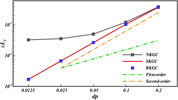
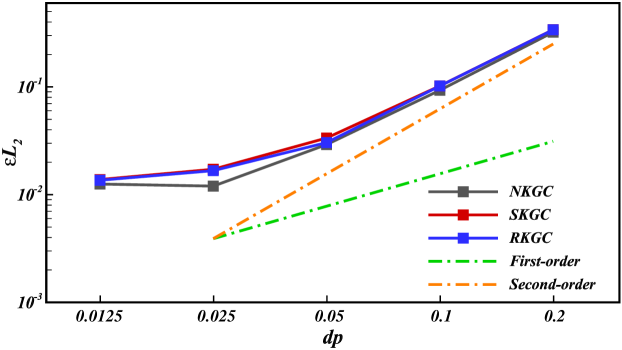
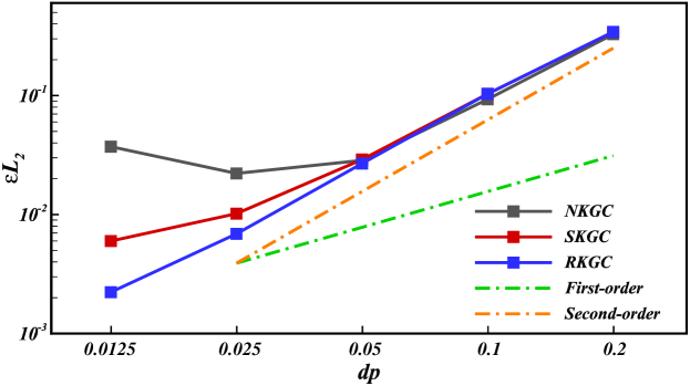
Figure 1: Convergence study of conservative approximations of the gradient at the $h=1.3\Delta x$. (a) Lattice distribution; (b) P relaxation; (c) B relaxation.

For lattice-distributed particles, as illustrated in Fig. 1, both corrected formulations achieve second-order convergence compared to the typical second-order-to-saturation behavior of NKGC. For the particles after the P relaxation, as depicted in Fig. 1, all formulations exhibit the second-order-to-saturation behavior, as the integration errors dominant at high-resolution independent of the kernel corrections. For particles after the B relaxation, as shown in Fig. 1 only RKGC maintains second-order convergence as expected from the analysis in section 3.1. At high resolutions, SKGC degrades to first-order as it fails to reproduce the linear gradient, and NKGC even suffers from increased error.

Furthermore, as depicted in Fig. 2, it is observed that, for RKGC, reducing the $h/\Delta x$ does not affect the convergence rate as long as the B relaxation is applied.

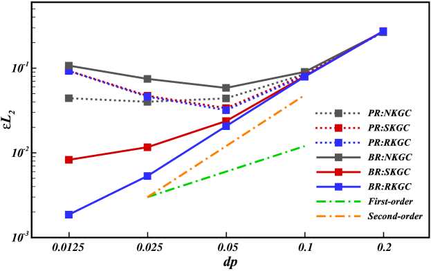
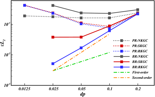
Figure 2: Convergence study of conservative approximations of the gradient at the reduced $h/\Delta x$ values. (a) $h=1.15\Delta x$; (b) $h=0.8\Delta x$.

This is not out of expectation since Eq. (21) is not explicitly dependent on smoothing length. In contrast, SKGC and NKGC suffer from serious degeneration or even increased error at high resolutions, no matter whether P or B relaxation is applied. Note that the data at $\Delta x=0.0125$ for $h=0.8\Delta x$ is missing for B relaxation as shown in Fig. 2. This is because, under the present straightforward relaxation stepping as given in Section 3.2, the B relaxation is not able to reach the convergence criterion. Such difficulty actually indicates the implicit limitation of the RKGC formulation. However, such limitation is generic and more demanding for high-order consistencies as shown latter, and even not unexpected since a basic requirement of consistent particle approximation is sufficient overlapping between the kernel supports of neighboring particles [48].

5 Numerical examples

In this section, the proposed RKGC formulation is applied to the WCSPH and ESPH methods with fully relaxed particles for the latter. Again, the C2 Wendland kernel is utilized, with the smoothing length set to be $h=1.3\Delta x$ if not specifically stated.

5.1 Taylor-Green vortex flow at Re=100

The incompressible Navier-Stokes equation offers an analytical time-dependent solution for this periodic array of vortices in a unit square domain as

$$\begin{cases}u\left(x,y,t\right)=-Ue^{bt}\cos\left(2\pi x\right)\sin\left(2\pi y\right)\\ v\left(x,y,t\right)=Ue^{bt}\sin\left(2\pi x\right)\cos\left(2\pi y\right)\end{cases}.$$ (27)

This solution serves as the initial velocity distribution at $t=0$ and acts as a benchmark to assess the simulation accuracy. The decay rate of the velocity field is determined by $b=-8\pi^{2}/Re$, where $Re=\rho UL/\eta$ represents the Reynolds number derived from the fluid density $\rho$, the maximum initial velocity $U$, the domain size $L$, and the viscosity $\eta$. In the current simulations, a domain size of $L=1$ is employed, with periodic boundary conditions applied in both coordinate directions. The maximum initial flow speed is set at $U=1$, and the Reynolds number is $Re=100$.

5.1.1 WCSPH results

The Taylor-Green vortex problem is first investigated using the WCSPH method, with the particle spacing $\Delta x=0.02$ ($50\times 50$ particles), $\Delta x=0.01$ ($100\times 100$ particles), and $\Delta x=0.005$ ($200\times 200$ particles). The initial particle distribution follows a lattice arrangement. Fig. 3 showcases the results obtained by employing the transport-velocity formulation in each advection time step.

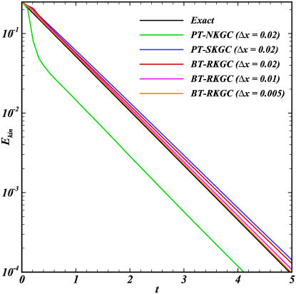
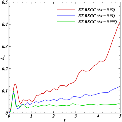
Figure 3: Taylor-Green Vortex: WCSPH results obtained with the transport-velocity formulations. (a) Decay of the kinetic energy; (b) Relative error of the maximum velocity (BT-RKGC).

Here, PT and BT denote the original and KGC transport-velocity formulations, respectively. The relative error of the maximum velocity $L_{\infty}^{\rm v}$ is defined as

$$L_{\infty}^{\rm v}=\left|\frac{{\rm max}(\boldsymbol{\rm v_{i}}(t))-Ue^{bt}}{Ue^{bt}}\right|.$$ (28)

Fig. 3 shows that the corrected formulations deliver superior results compared to PT-NKGC, where no correction is employed. Specifically, BT-RKGC yields the most favorable outcomes, indicating improved accuracy. Moreover, as the resolution increases, the kinetic energy obtained by BT-RKGC converges toward the analytical solutions. Such convergence is also demonstrated in Fig. 3 through the relative error of the maximum velocity.

5.1.2 ESPH results

In the ESPH simulations, the particle distributions are initialized through relaxation, ensuring that the zero-order consistency residue diminishes to less than $1\times 10^{-5}$ for P and B relaxations in SKGC and RKGC, respectively. The initial particle spacing is varied as $\Delta x=0.04$ ($25\times 25$ particles), $\Delta x=0.02$ ($50\times 50$ particles), and $\Delta x=0.01$ ($100\times 100$ particles) to analyze the influence of the resolution. Fig. 4 presents the decay of the kinetic energy $E_{\text{kin}}$ and its relative error $L_{\infty}^{E}$ defined by

$$L_{\infty}^{E}=\left|\frac{E_{\text{kin}}(t)-E_{\text{kin}}^{a}(t)}{E_{\text{kin}}^{a}(t)}\right|,$$ (29)

where $E_{\text{kin}}^{a}$ represents the analytical kinetic energy with a decay rate of $-16\pi^{2}/Re$.

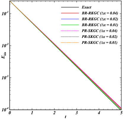
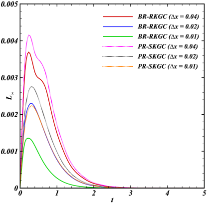
Figure 4: Taylor-Green Vortex: ESPH results obtained with the relaxed particles. (a) Decay of the kinetic energy; (b) Relative error of the kinetic energy.

Both SKGC and RKGC produce results converging to the analytical solution, while RKGC achieves lower kinetic energy error across all resolutions and exhibits improved accuracy compared to that of SKGC.

5.2 Lid-driven cavity at Re=1000

The lid-driven cavity problem serves as a well-known and challenging test case for the SPH method. In this scenario, a wall-bounded unit square cavity is presented, with its top wall moving at a constant speed of $U_{\text{wall}}=1$. For the flow at a Reynolds number of $Re=1000$, we reference the high-resolution multi-grid results of Ghia et al. [49], who utilized the finite difference method on a $257\times 257$ mesh.

5.2.1 WCSPH results

The results obtained by the WCSPH method are presented in Fig. 5.

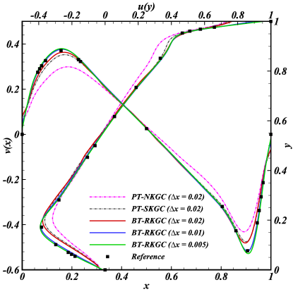
Figure 5: Lid-driven cavity: WCSPH results obtained with the transport-velocity formulations. (a) Velocity profiles along the horizontal and vertical central lines; (b) Velocity fields (visualized by the magnitude ranging from 0 to 1) with vectors obtained by BT-RKGC at the $\Delta x=0.01$.

The comparison of velocity profiles with the reference results, depicted in Fig. 5, reveals that corrected formulations yield results more closely aligned with the reference than PT-NKGC formulation without correction. Furthermore, BT-RKGC outperforms PT-SKGC. As resolution increases, results obtained by BT-RKGC demonstrate clear convergence and good agreement with the reference. The magnitude of the velocity and the velocity vectors of the flow field shown in Fig. 5 exhibit a smoothed distribution and typical vortical structures, such as those induced by the shear force of the moving wall and the single-core vortex located at the center of the cavity, consistent with findings presented in Refs. [49, 33, 50].

5.2.2 ESPH results

Again, the ESPH results are obtained on fully relaxed initial particle distributions at smoothing lengths of $h=1.3\Delta x$ and $h=1.15\Delta x$, as illustrated in Fig. 6..

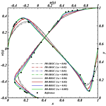
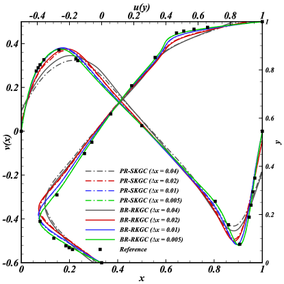
Figure 6: Lid-driven cavity: ESPH method results for velocity profiles along the horizontal and vertical central lines at different smoothing lengths. (a) $h=1.3\Delta x$; (b) $h=1.15\Delta x$.

It is observed that the BR-RKGC produces results closer to the reference than the PR-SKGC at the low resolutions, i.e., $\Delta x=0.04$ and $\Delta x=0.02$, indicating less integration errors. With the resolution increased, both methods could yield converged results, and the error difference is small due to the sufficient smoothing length.

Fig. 7 presents the obtained velocity fields with vectors when the smoothing length is decrease to $h=0.8\Delta x$.

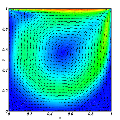
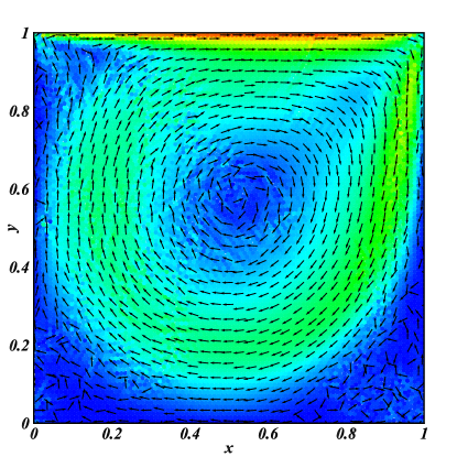
Figure 7: Lid-driven cavity: ESPH method results for velocity fields (visualized by the magnitude ranging from 0 to 1) with vectors at $h=0.8\Delta x$ and $\Delta x=0.01$. (a) BR-RKGC; (b) PR-SKGC.

As discussed in Section 4, the RKGC formulation combined with the B relaxation achieves the first-order consistency, not explicitly relying on the smoothing length, while the SKGC one suffers serious degeneration. Therefore, as presented in Fig. 7, the BR-RKGC is still able to generate the smooth velocity distribution and captures the key flow characteristics, aligning with the reference results [49, 51] and the one displayed in Fig. 5 obtained by the WCSPH method. Moreover, the secondary vortices in the lower and upper corners are still well-identified. However, the PR-SKGC, as presented in Fig. 7, fails to yield a reasonable smooth velocity distribution, with velocity oscillation and noise, especially at the upper-left corner vortex and around the single-core vortex. The velocity vectors at the lower corners also failed to capture the secondary vortices. Therefore, the proposed RKGC formulation and B relaxation could still achieve improved accuracy and good convergence, even with a reduced $h/\Delta x$ value. Note that, in practical viscous flow simulations, while the RKGC aims to achieve first-order consistency for gradient and divergence operators, the numerical results do not necessarily always maintain it because the Laplacian operator in SPH approximations does not precisely satisfy first-order consistency yet, and the adoption of the Riemann solver may also degenerate the consistency as the RKGC is only applied on the non-dissipative terms.

5.3 Standing wave

The standing wave problem serves as a typical benchmark for evaluating the accuracy of the SPH method in addressing free-surface problems. In this section, a two-dimensional standing wave problem is investigated using the WCSPH method. The initial configuration, as depicted in Fig. 8,

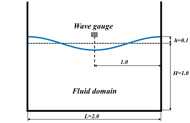
Figure 8: Standing wave: Initial configuration of the simulation.

defines the initial free surface according to

$$\eta_{0}=A\cos(k(x+\lambda)/2).$$ (30)

Here, the parameters are set as follows: the wave amplitude $A$ = $0.1H$, with an average water depth of $H=1.0$; the wave number $k=2\pi/\lambda$, and the wavelength $\lambda=2.0$. The initial velocity of the particles is set to be zero. Note that transport velocity formulations are not employed here (also for other free-surface flows in this work) following the general practice of SPH simulations [18, 52, 38]. The study evaluates the free-surface elevation at the central position, and compare it against the second-order analytical solution proposed by Wu et al. [53]. In order to maintain numerical stability, the KGC matrix near the free surface is weighted by the identity matrix (WKGC¹), as suggested in Ref. [38], with the constant parameter $\alpha=0.5$ for all free-surface flow problems in the current study.

Fig. 9 illustrates the decay of the normalized mechanical energy across different formulations and compares them with the analytical and reference results.

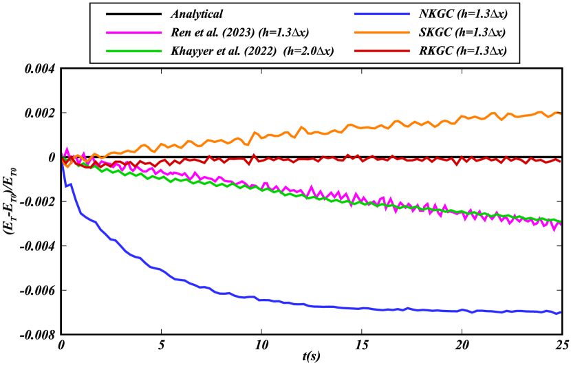
Figure 9: Standing wave: Time evolution of the decay of the normalized mechanical energy obtained by different formulations ($\Delta x=0.01$).

It is observed that the RKGC formulation is able to preserve the energy very well, suggesting very small numerical dissipation. However, NKGC exhibits rapid energy decay, even when the smoothing length is increased to $h=2.0\Delta x$, as shown by Khayyer et al. [54]. It is also noted that the SKGC formulation leads to an increase in the energy, consistent with findings from Ref. [38, 52]. Therefore, extra weight with the identity matrix (as WKGC² in Ref. [38]) is added to decrease the contribution of the SKGC formulation to eliminate the artifact but, as illustrated in Fig. 9, it still shows considerable energy loss.

Fig. 10 illustrates the wave heights across different methods as well as the convergence analysis of the RKGC formulation.

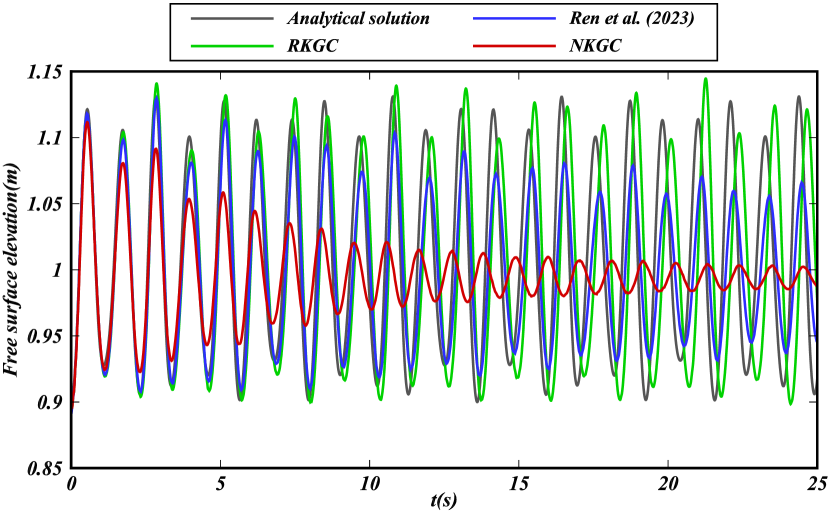
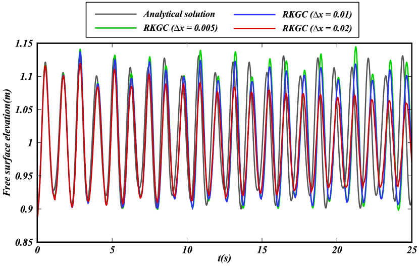
Figure 10: Standing wave: Time evolution of the free-surface elevation at the center of the tank. (a) Comparison across different formulations ($\Delta x=0.005$); (b) Convergence study of the RKGC formulation.

The comparisons of the wave height depicted in Fig. 10 indicate that while the results obtained with both SKGC and RKGC achieve notable improvements compared to NKGC, RKGC further improves accuracy considerably and generates closer approximations to the analytical solution. As displayed in Fig. 10, RKGC demonstrates good convergence with increasing resolution.

5.4 Oscillating drop

The two-dimensional oscillating drop was also investigated to evaluate the energy conservation properties of the proposed method. This problem, as outlined in Ref. [55] and depicted in Fig. 11, involves a drop with a radius of $R=1$ immersed in an assumed inviscid fluid.

Figure 11: Oscillating drop: Schematic illustration of the benchmark test.

This drop experiences a central conservative force $F=-\Omega^{2}R$ and is initialized with a velocity profile defined by

$$\begin{cases}u_{0}=A_{0}x\\ v_{0}=-A_{0}y\end{cases},$$ (31)

where $A_{0}=1.0$ and $A_{0}/\Omega=1.0$. The analytical solution reported in Ref. [56] is referenced for quantitative comparison and validation.

The pressure contours at two different instants are illustrated in Fig. 12, showcasing the robust free-surface profile and smooth pressure fields obtained by RKGC.

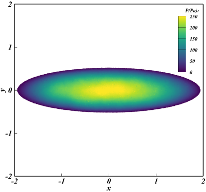
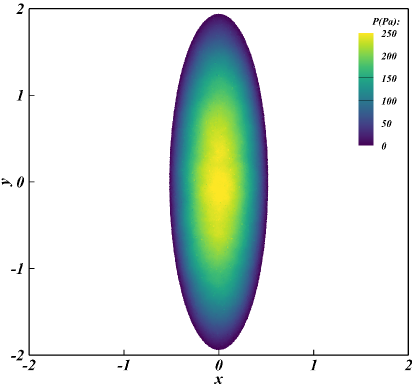
Figure 12: Oscillation drop: Snapshots of the free-surface profile and the pressure contour obtained by the RKGC. (a) t=20.5s; (b)t=22.9s.

Furthermore, Fig. 13 illustrates pressure observations at the center of the domain obtained by the RKGC for different resolutions. It shows that the RKGC has good numerical stability and accuracy. As the resolutions increase, they converge and indicate a good convergence property.

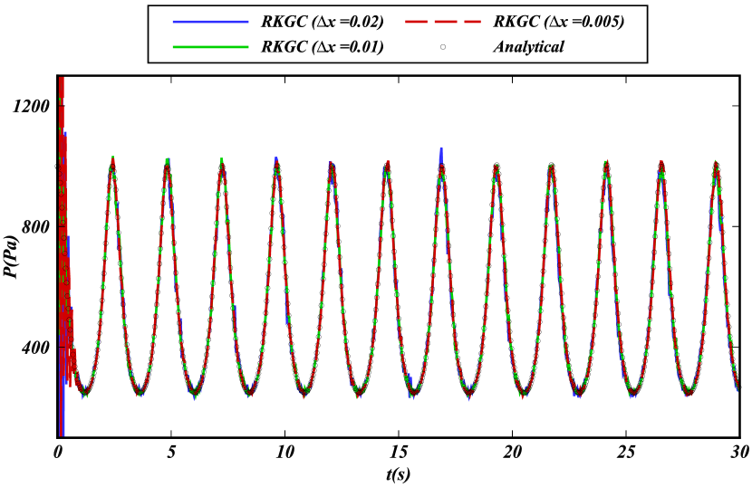
Figure 13: Oscillating drop: Time history of the pressure at the drop center obtained by the RKGC with different particle resolutions.

Fig. 14 presents the time evolution of the decay of normalized mechanical energy across different formulations and compares them with the analytical and reference results.

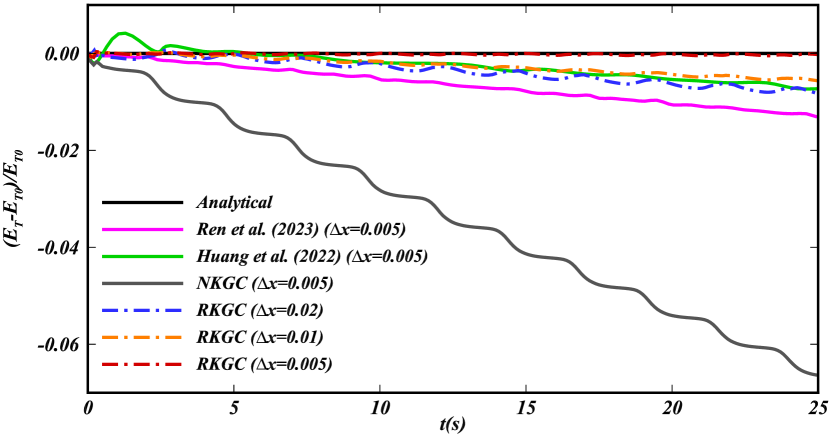
Figure 14: Oscillating drop: Time evolution of the decay of the normalized mechanical energy obtained by different formulations.

Aligning with the observation in Fig. 9, the RKGC formulation is able to preserve the energy quite well, even at a low resolution, and the energy conservation properties are improved with the resolution increase. It indicates there is no evident energy decay at the resolution of $\Delta x=0.005$. However, at this high resolution, NKGC still exhibits a considerably high decay rate of the energy. While the corrected formulations introduced by Ren et al. [38] and Huang et al. [42] achieve notable reduction of the energy decay, they still suffer more energy loss than that obtained by RKGC at a lower resolution. The separate comparisons of kinetic and potential energies are depicted in Fig. 15.

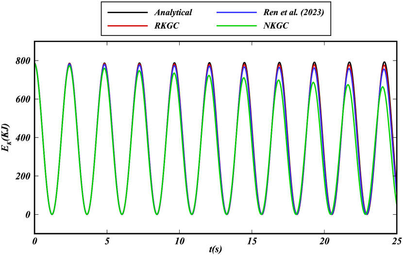
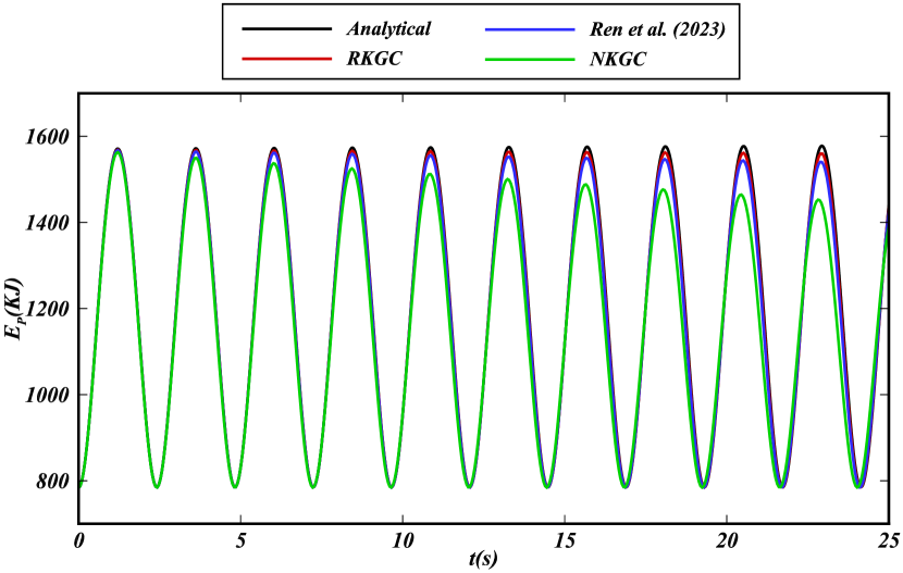
Figure 15: Oscillating drop: Time history of the energy obtained by different formulations ($\Delta x=0.01$). (a) Kinetic energy; (b) Potential energy.

The corrected formulations all show improved alignment with the analytical solution compared to the NKGC for both kinetic and potential energies. Moreover, RKGC exhibits a closer agreement with the analytical solution than those reported in Ref. [38] where a corrected formulation is also adopted.

5.5 Dam-break flow

The dam-break flow, extensively explored both experimentally [57, 58, 59, 60] and numerically [61, 62, 5, 47], is a challenging benchmark to validate the SPH method. Fig. 16 depicts the initial configuration for the simulation, aligning with the experimental setup outlined by Lobovsky et al. [60].

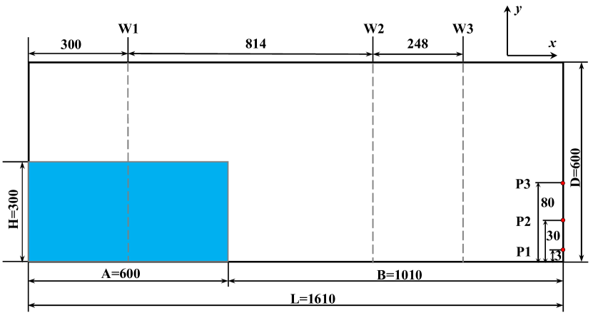
Figure 16: Dam-break flow: Initial configuration of the simulation.

Three measurement points (W1, W2, and W3) are assigned to record the free surface height, and three probes (P1, P2, and P3) are employed to capture the pressure signals. We consider an inviscid flow with a density of $\rm\rho_{0}=1000kg/m^{3}$ and a gravitational constant of $\rm g=9.8m/s^{2}$. According to the shallow water theory [63], the maximum velocity is estimated as $2\sqrt{gH}$ to determine the speed of sound, where $H$ represents the initial water depth.

Fig. 17 shows several typical snapshots of the time evolution of the free surface obtained by the RKGC formulation.

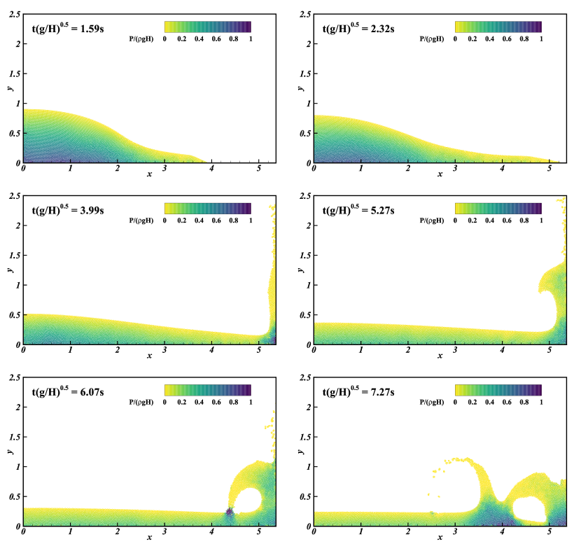
Figure 17: Dam-break flow: Snapshots of particles and pressure distributions during the time evolution with $H/\Delta x=60$.

The obtained results demonstrate smooth pressure distributions and robust free-surface profiles and align well with experimental observations [60] and previously reported simulation results [5, 47, 38]. RKGC could appropriately capture key flow characteristics, including high roll-up along the downstream wall, a prominently reflected jet, and free surface disruption caused by the arrival of the secondary wave. Fig. 18 shows the predicted propagation of the surge-wave front, along with comparisons to data measured in various experiments [58, 57, 60] and the analytical solution derived from the shallow-water equation [63].

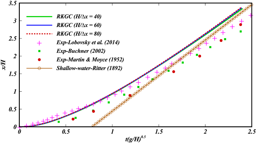
Figure 18: Dam-break flow: Time evolution of the surge-wave front.

It is observed that the present predictions have good convergence and agree well with the experiments before $t\sqrt{gH}<1$, aligning closely with the analytical solution afterward, but overestimate the front speed obtained from the experiments, which was also observed in other simulations [61, 64, 5].

The comparisons of the water levels recorded at W1, W2, and W3 with experimental observations obtained from Ref. [60] are presented in Fig. 19.

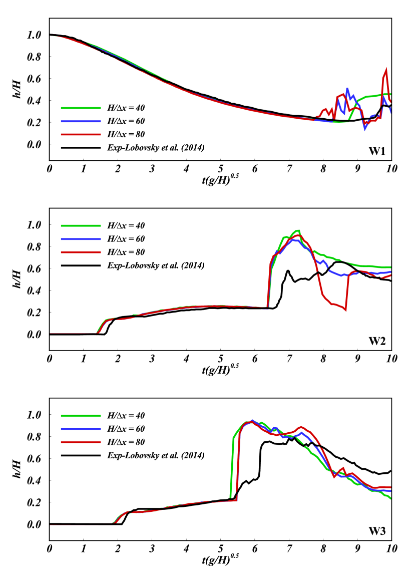
Figure 19: Three-dimensional dam-break: water levels recorded at W1, W2, and W3. Convergence study and comparison against experimental results presented by Lobovsky et al. [60].

The wave height exhibits good agreement with the experimental data. Nonetheless, we observe discrepancies in higher run-up waves (W1) and marginally faster wavefront (W2 and W3) in the current results. Similar observations were also reported in previous numerical studies [61, 5, 38], potentially attributed to the adoption of inviscid flow in the current study, leading to violent wave breaking up and splashing. The history of pressure signals recorded at P1, P2, and P3 is presented in Fig. 20.

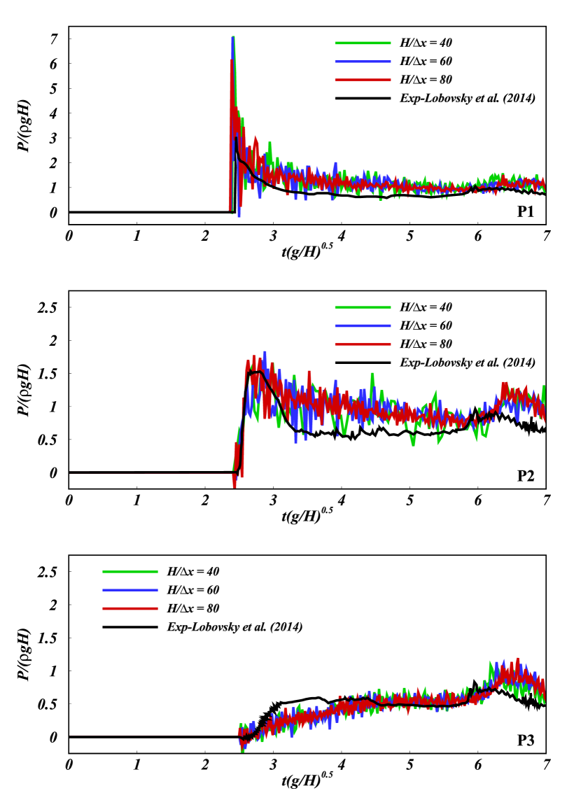
Figure 20: Three-dimensional dam-break: history of pressure signals recorded at probes P1, P2 and P3. Convergence study and comparison against experimental results presented by Lobovsky et al. [60].

The current results have good agreement with the experimental observations [60], except for observed pressure fluctuations in the current study resulting from the weakly compressible assumption, which tend to decrease with increasing spatial resolutions. Discrepancies in pressure magnitudes at P2 and P3 were also reported in other studies [62, 47] where different WCSPH methods were employed. The overestimated pressure peak at P2 by the current method is potentially due to the weakly compressible model. In addition, the air cushion effect in the experiment may also decrease its pressure peak [60]. The occurrence time of the pressure observation at P3 aligns with $t\sqrt{g/H}\approx 2.7$ very well, though the peak value is underestimated.

Following the definition of the dissipation of total mechanical energy [65]:

$$\Delta E=\frac{E-E_{0}}{E_{0}-E_{\infty}},$$ (32)

where $E$ the total mechanical energy, $E_{0}$ is the initial mechanical energy, and $E_{\infty}$ is the mechanical energy after reaching the equilibrium state. Fig. 21 displays the evolution of the mechanical energy of RKGC, and compares it with SKGC and different references.

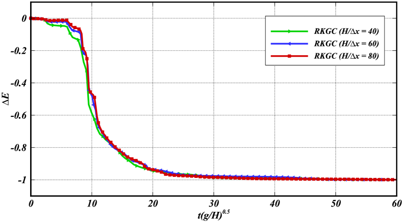
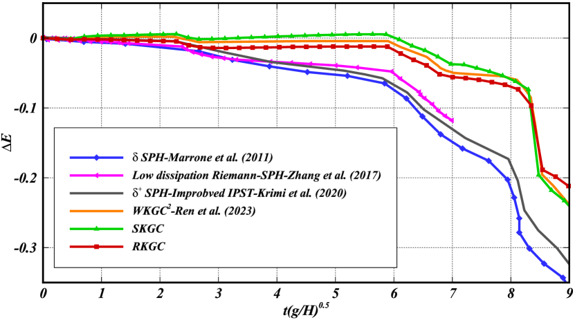
Figure 21: Dam-break flow: evolution of mechanical energy. (a) Global evolution; (b) Zoom in on the initial evolution and compare with references ($H/\Delta x=80$).

Fig. 21 shows that with increased resolutions, the numerical dissipation decreases rapidly. It is observed in Fig. 21 that RKGC has lower energy decay compared to other numerical results [65, 5, 66], where no correction was employed. SKGC results in energy increasing before the splashing ($t\sqrt{gH}<6$), and involving the extra weighting of the KGC employed by Ren et al. [38] could alleviate this issue, but it still leads to an energy increase before the roll-up wave ($t\sqrt{gH}<2.3$). However, RKGC could maintain the energy before the splashing and leads to a slightly lower energy decay rate afterwards compared to SKGC and the results in Ref. [38], except for the energy-increasing artifacts observed for the latter.

5.6 Three-dimensional oscillating wave surge converter (OWSC)

As a forefront wave energy converter, the oscillating wave surge converter (OWSC) has showcased remarkable energy absorption capabilities and hydrodynamic performance, and it has been widely studied with numerical and experimental methods [67, 68, 69, 70]. In this section, the three-dimensional OWSC is investigated with the RKGC formulation. Fig. 22 illustrates the configurations of the wave tank and the OWSC model, which are identical to the experimental setup detailed in Ref. [68].

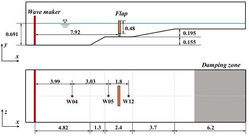
Figure 22: OWSC: Schematic depiction of the wave tank and the OWSC model.

The wave tank measures 18.42 m in length, 4.58 m in width, and 1.0 m in height. The OWSC device is simplified as a flap with dimensions of 0.48 m in height, 1.04 m in width, and 0.12 m in thickness, and is hinged to a base with a height of 0.16 m. The flap has a mass of 33 kg, and its angular inertia is 1.84 $\rm kg/m^{2}$. To measure the wave elevation and impact pressure on the flap, three wave gauges, as shown in Fig. 22, and six pressure sensors, whose positions are listed in Table 1, are employed. Note that the present model is 1:25 scaled to that in the Ref. [68], and all the results present in this work have been converted to the full scale accordingly.

Table 1: OWSC: Pressure sensor positions on the front flap along the z-axis from the device’s center, with $y=0$ representing the mean water level.

No.	y-axis(m)	z-axis(m)	No.	y-axis(m)	z-axis(m)
P01	-0.046	0.468	P09	-0.117	0.156
P03	0.050	0.364	P11	0.025	0.052
P05	-0.300	0.364	P13	-0.239	0.052

Considering the regular wave with a height $H=5$m and a period $T=10$s at full scale, a piston-type wave maker is employed to generate regular waves, adopting an ensemble of dummy particles whose motion follows the linear wavemaker theory [71], where the particle displacement in $x$-direction $x_{a}$ is determined by

$$x_{a}=S\sin(ft+\phi),$$ (33)

with $S$ the wave stroke, $f$ the wave frequency, and $\phi$ the initial phase. The wave stroke is further defined as

$$S=\dfrac{H\sinh(2kh_{0})+2kh_{0}}{\sinh(2kh_{0})\tanh(kh_{0})},$$ (34)

where $h_{0}$ is the water depth, and $k$ is the wave number. To minimize wave reflection effects, a damping zone [72] as illustrated in Fig. 22, is established at the end of the wave tank. Within this damping zone, the particle velocity undergoes decay according to

$$\boldsymbol{\rm v}=\boldsymbol{\rm v_{0}}\left(1.0-\Delta t\theta\left(\dfrac{\boldsymbol{\rm r-r_{0}}}{\boldsymbol{\rm r_{1}-r_{0}}}\right)\right).$$ (35)

Here, $\boldsymbol{\rm v_{0}}$ the initial velocity of the fluid particle at the entry of the damping zone, $\boldsymbol{\rm v}$ the velocity after damping, $\Delta t$ the time step, and $\boldsymbol{\rm r_{0}}$ and $\boldsymbol{\rm r_{1}}$ are the initial and final positions of the damping zone, respectively. The reduction coefficient $\theta=5.0$ governs the modifications on the velocity at each time step in the current simulation. The entire system is discretized with a particle spacing of 0.03 m, resulting in 1.542 million fluid particles and 0.628 million solid particles. The present numerical results have been compared with both experimental observations and numerical investigations reported in Ref. [68].

Fig. 23 displays snapshots of the free-surface profile colored by the normalized pressure 23 and velocity magnitude 23, respectively.

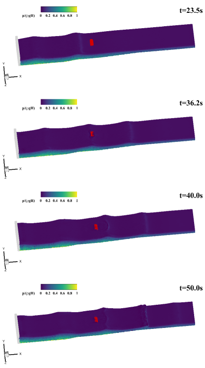
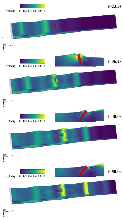
Figure 23: OWSC: Snapshots of free surfaces and the flap motion during time evolution. (a) Fluid particles are colored by the normalized pressure; (b) Fluid particles are colored by the velocity magnitude.

The results clearly demonstrate that the current method effectively captures the dynamic free-surface elevation, including wave reflection and breaking around the flap. Additionally, the outcomes exhibit smooth pressure and velocity fields, even during the intensive wave interactions around the flap, where wave reflection and breaking are observed. Furthermore, the cross-sectional slices along the middle line provide insights into the rotational state of the flap. These observations are consistent with those reported in the references [68, 70], as evidenced by the wave height and flap rotation angle history presented below.

The observed wave evaluations are depicted in Fig. 24, offering a comparison with the reference results [68, 38].

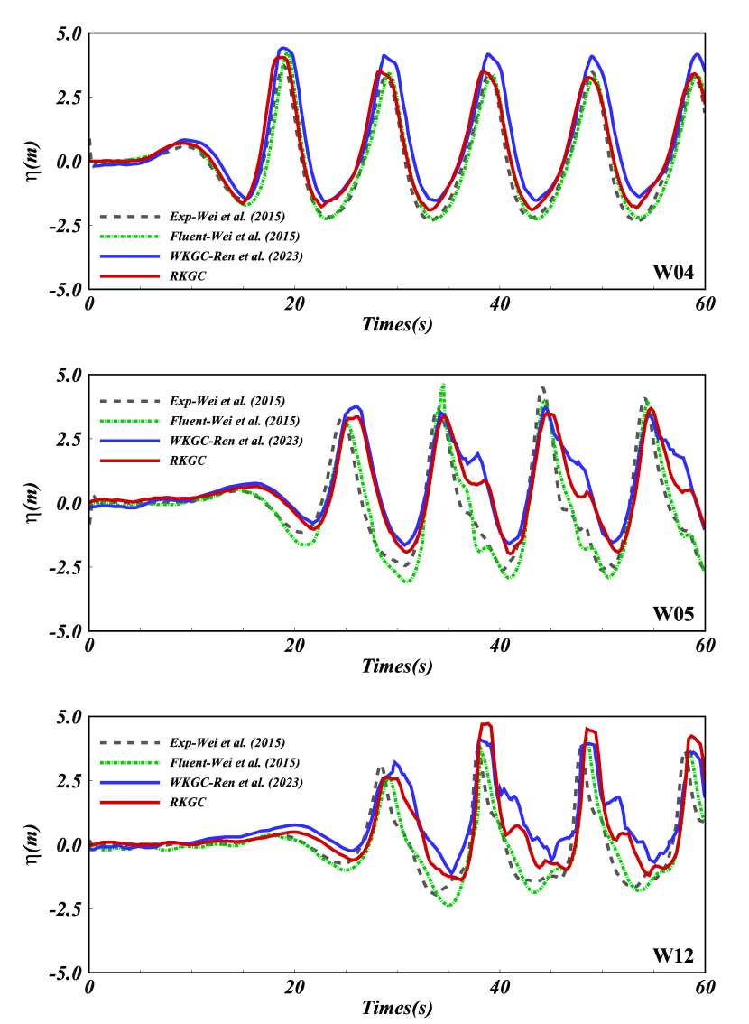
Figure 24: OWSC: Comparison of free surface elevations for wave height $H=5.0m$ and period $T=10.0s$ against results of Wei et al. [68] and Ren et al. [38].

The RKGC formulation demonstrates good agreement with the results obtained from experiments, particularly at locations W04 and W05, which are in the seaward direction from the flap. However, discrepancies, especially the overestimation of wave crest height, are noticeable at location W12, positioned behind the flap. These differences may arise from wave reflection and breaking around the flap. Additionally, the absence of a turbulence model in the current study also contributes to these observations, as the reference numerical results [68] utilize a turbulence model, introducing additional numerical dissipation. Compared to the results in Ref. [38] where WKGC² is adopted, RKGC shows better alignment with experimental, particularly predicting more accurate wave heights at W04 and W05 positions and wave falls at all three positions.

Fig. 25 presents the rotation angle of the flap, providing a comparison with the experimental observations and other numerical predictions.

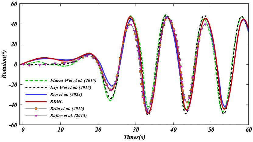
Figure 25: OWSC: Comparison of the time evolution of the flap rotation.

The comparison underscores the good agreement with the experimental and Fluent results [68]. While predictions obtained by standard SPH formulations without corrections, such as those reported in Ref. [67, 69], often underestimate the extreme rotation angle of the flap compared to experimental results, the prediction gained with the RKGC formulation and WKGC² [38] notably overcomes this limitation. They provide more accurate predictions for flap rotating angles, aligning more closely with the experimental observations. The RKGC formulation in this study is applied only in the fluid domain rather than the fluid-structure interaction, thus, it gives slightly closer predictions to experiments than that in Ref. [38].

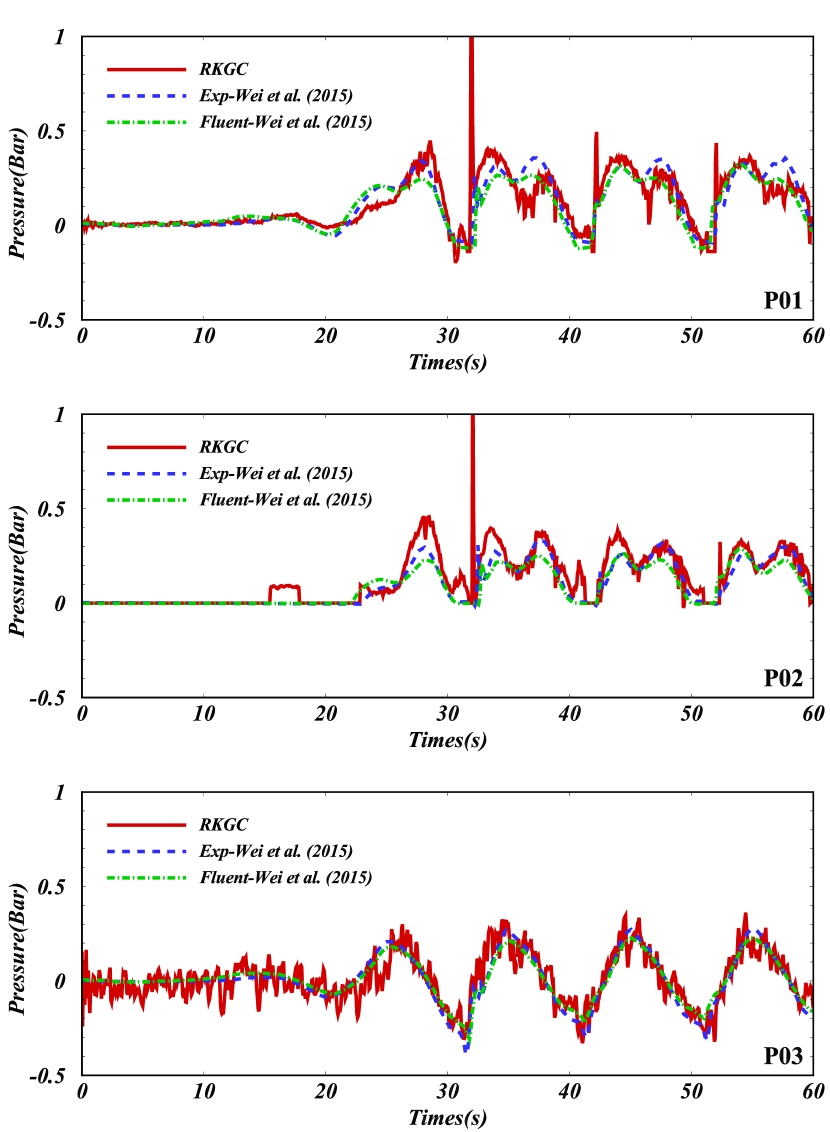
Figure 26:

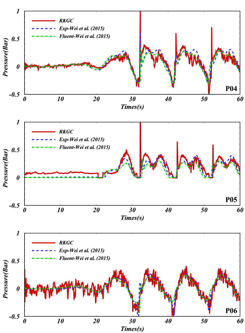
Figure 27: OWSC: Comparison of wave load time histories on the flap for $H=5.0m$ and $T=10.0s$ against the results of Wei et al. [68].

The pressure evolution over time at each probe on the flap is illustrated and compared in Fig. 27. The results obtained using the RKGC formulation align well with the experimental data, predicting reasonable slamming pressures despite some pressure oscillations due to the weakly compressible assumption. Compared to the pressure results in Ref. [70, 38] based on the SPH method, the current observed pressure shows fluctuations due to the density reinitialization method employed in Ref. [73], which has been proven more suitable for free-surface problems. Moreover, the RKGC method predicts pressures that are more consistent with experimental results than those obtained using Fluent. This includes capturing higher double pressure peaks at P01, P02, and P05, as well as the lower pressure drops at P03 and P06. However, some discrepancies still exist, which may be attributed to air entrainment in the splash passing the flap, a factor not considered in the current method.

6 Extension

Indeed, the concept of the reverse KGC formulation can be readily extended to accommodate second- or even higher-order consistency conditions of the SPH gradient approximation. This extension uses the correction function for RKPM proposed by Liu et al. [21, 22], provided that the corresponding particle relaxation is employed. The SPH gradient approximation in the non-conservative form can be expressed similarly to Eq. (9) as

$$\nabla\psi_{i}=\sum_{j}\psi_{ij}\boldsymbol{C_{i}}\left(\boldsymbol{\rm r}_{i},\boldsymbol{\rm r}_{j}\right)\nabla W_{ij}V_{j},$$ (36)

where $\boldsymbol{C_{i}}\left(\boldsymbol{\rm r}_{i},\boldsymbol{\rm r}_{j}\right)={C}_{0}\left(\boldsymbol{\rm r}_{i}\right)+\boldsymbol{C_{1}}\left(\boldsymbol{\rm r}_{i}\right)\left(\boldsymbol{\rm r}_{j}-\boldsymbol{\rm r}_{i}\right)$ represents the correction function (see Refs. [21, 22] for more definitions). Following Taylor expansion of $\psi_{j}$ and substituting it into (36), one can obtain

$$\nabla\psi_{i}=-\sum_{j}\left(\nabla\psi_{i}\cdot\boldsymbol{\rm r}_{ij}+\frac{1}{2}\nabla\cdot\nabla\psi_{i}:\boldsymbol{\rm r}_{ij}\otimes\boldsymbol{\rm r}_{ij}\right)\boldsymbol{C_{i}}\left(\boldsymbol{\rm r}_{i},\boldsymbol{\rm r}_{j}\right)\nabla W_{ij}V_{j}.$$ (37)

To vanish the leading moments and ensure second-order consistency, the following conditions should be satisfied simultaneously:

$$\begin{cases}\displaystyle\sum_{j}-\boldsymbol{\rm r}_{ij}\otimes\boldsymbol{C_{i}}\left(\boldsymbol{\rm r}_{i},\boldsymbol{\rm r}_{j}\right)\nabla W_{ij}V_{j}=\mathbf{I}\\ \displaystyle\sum_{j}\boldsymbol{\rm r}_{ij}\otimes\boldsymbol{\rm r}_{ij}\cdot\boldsymbol{C_{i}}\left(\boldsymbol{\rm r}_{i},\boldsymbol{\rm r}_{j}\right)\nabla W_{ij}V_{j}=\mathbf{0}\end{cases}.$$ (38)

Subsequently, $C_{0}$ and $\boldsymbol{C_{1}}$ can be obtained by solving Eq. (38). Consequently, the reverse-corrected conservative formulation with second-order consistency can be written similarly to Eq. (22) as

$$\nabla\psi_{i}=-\sum_{j}\left(\psi_{i}\boldsymbol{C_{j}}+\psi_{j}\boldsymbol{C_{i}}\right)\nabla W_{ij}V_{j},$$ (39)

which can be further rewritten as

$$\nabla\psi_{i}=-\psi_{i}\sum_{j}\left(\boldsymbol{C_{i}}+\boldsymbol{C_{j}}\right)\nabla W_{ij}V_{j}+\sum_{j}\psi_{ij}\boldsymbol{C_{i}}\nabla W_{ij}V_{j}.$$ (40)

The first term on the RHS can also be nullified by particle relaxation based on the correction function, while the second term accurately reproduces the gradient as indicated in Eq. (36). Therefore, the reverse-corrected conservative formulation in Eq. (39) could continuously exhibit second-order consistency. However, obtaining the corresponding correction function and achieving convergence in the particle relaxation driven by the correction function to fulfill second-order consistency still presents significant challenges.

7 Conclusion

This paper introduces the reverse KGC (RKGC) formulation, which is conservative and, integrating the particle relaxation based on the KGC matrix, ensures the zero- and first-order consistencies without explicit dependence on smoothing length. The implementations in typical SPH methods, including Lagrangian SPH and Eulerian SPH, exhibited considerably improved accuracy, especially good energy conservation properties in general free-surface problems. While acknowledging the ease of extending the scheme to high-order consistency, one expects future work to address the persistent challenges in achieving converged solutions for particle relaxation driven by the KGC matrix and high-order correction function, especially for three-dimensional complex geometries and the situation employing a $h/\Delta x$ value smaller than 1.0. Additionally, extending RKGC for SPH solid dynamics and to a similar idea for Laplacian operators is to be considered as future work.

References

- [1] L. B. Lucy, A numerical approach to the testing of the fission hypothesis, Astronomical Journal, vol. 82, Dec. 1977, p. 1013-1024. 82 (1977) 1013–1024.
- [2] R. A. Gingold, J. J. Monaghan, Smoothed particle hydrodynamics: theory and application to non-spherical stars, Monthly notices of the royal astronomical society 181 (3) (1977) 375–389.
- [3] J. J. Monaghan, Simulating free surface flows with sph, Journal of computational physics 110 (2) (1994) 399–406.
- [4] X. Y. Hu, N. A. Adams, A multi-phase sph method for macroscopic and mesoscopic flows, Journal of Computational Physics 213 (2) (2006) 844–861.
- [5] C. Zhang, X. Hu, N. A. Adams, A weakly compressible sph method based on a low-dissipation riemann solver, Journal of Computational Physics 335 (2017) 605–620.
- [6] W. Benz, E. Asphaug, Simulations of brittle solids using smooth particle hydrodynamics, Computer physics communications 87 (1-2) (1995) 253–265.
- [7] T. Rabczuk, J. Eibl, Simulation of high velocity concrete fragmentation using sph/mlsph, International Journal for Numerical Methods in Engineering 56 (10) (2003) 1421–1444.
- [8] Y.-X. Peng, A.-M. Zhang, F.-R. Ming, S.-P. Wang, A meshfree framework for the numerical simulation of elasto-plasticity deformation of ship structure, Ocean Engineering 192 (2019) 106507.
- [9] T. Ye, D. Pan, C. Huang, M. Liu, Smoothed particle hydrodynamics (sph) for complex fluid flows: Recent developments in methodology and applications, Physics of Fluids 31 (1) (2019) 011301.
- [10] H. Gotoh, A. Khayyer, On the state-of-the-art of particle methods for coastal and ocean engineering, Coastal Engineering Journal 60 (1) (2018) 79–103.
- [11] C. Zhang, M. Rezavand, X. Hu, A multi-resolution sph method for fluid-structure interactions, Journal of Computational Physics 429 (2021) 110028.
- [12] D. A. Fulk, A numerical analysis of smoothed particle hydrodynamics, Air Force Institute of Technology, 1994.
- [13] D. A. Fulk, D. W. Quinn, An analysis of 1-d smoothed particle hydrodynamics kernels, Journal of Computational Physics 126 (1) (1996) 165–180.
- [14] N. J. Quinlan, M. Basa, M. Lastiwka, Truncation error in mesh-free particle methods, International Journal for Numerical Methods in Engineering 66 (13) (2006) 2064–2085.
- [15] S. Litvinov, X. Hu, N. A. Adams, Towards consistence and convergence of conservative sph approximations, Journal of Computational Physics 301 (2015) 394–401.
- [16] J. J. Monaghan, Smoothed particle hydrodynamics, Annual review of astronomy and astrophysics 30 (1) (1992) 543–574.
- [17] V. G. Maz’ia, G. Schmidt, Approximate approximations, no. 141, American Mathematical Soc., 2007.
- [18] G. Oger, M. Doring, B. Alessandrini, P. Ferrant, An improved sph method: Towards higher order convergence, Journal of Computational Physics 225 (2) (2007) 1472–1492.
- [19] P. Randles, L. D. Libersky, Smoothed particle hydrodynamics: some recent improvements and applications, Computer methods in applied mechanics and engineering 139 (1-4) (1996) 375–408.
- [20] J. Chen, J. Beraun, T. Carney, A corrective smoothed particle method for boundary value problems in heat conduction, International Journal for Numerical Methods in Engineering 46 (2) (1999) 231–252.
- [21] W. K. Liu, S. Jun, Y. F. Zhang, Reproducing kernel particle methods, International journal for numerical methods in fluids 20 (8-9) (1995) 1081–1106.
- [22] W. K. Liu, S. Jun, S. Li, J. Adee, T. Belytschko, Reproducing kernel particle methods for structural dynamics, International Journal for Numerical Methods in Engineering 38 (10) (1995) 1655–1679.
- [23] M. Liu, G.-R. Liu, Restoring particle consistency in smoothed particle hydrodynamics, Applied numerical mathematics 56 (1) (2006) 19–36.
- [24] R. Batra, G. Zhang, Analysis of adiabatic shear bands in elasto-thermo-viscoplastic materials by modified smoothed-particle hydrodynamics (msph) method, Journal of computational physics 201 (1) (2004) 172–190.
- [25] G. Zhang, R. Batra, Modified smoothed particle hydrodynamics method and its application to transient problems, Computational mechanics 34 (2) (2004) 137–146.
- [26] S. Sibilla, An algorithm to improve consistency in smoothed particle hydrodynamics, Computers & Fluids 118 (2015) 148–158.
- [27] A. M. Nasar, G. Fourtakas, S. J. Lind, J. King, B. D. Rogers, P. K. Stansby, High-order consistent sph with the pressure projection method in 2-d and 3-d, Journal of Computational Physics 444 (2021) 110563.
- [28] S. N. Atluri, J. Cho, H.-G. Kim, Analysis of thin beams, using the meshless local petrov–galerkin method, with generalized moving least squares interpolations, Computational mechanics 24 (5) (1999) 334–347.
- [29] N. Flyer, B. Fornberg, Radial basis functions: Developments and applications to planetary scale flows, Computers & Fluids 46 (1) (2011) 23–32.
- [30] J. King, S. J. Lind, A. M. Nasar, High order difference schemes using the local anisotropic basis function method, Journal of Computational Physics 415 (2020) 109549.
- [31] N. Trask, M. Perego, P. Bochev, A high-order staggered meshless method for elliptic problems, SIAM Journal on Scientific Computing 39 (2) (2017) A479–A502.
- [32] Y. Zhu, C. Zhang, Y. Yu, X. Hu, A cad-compatible body-fitted particle generator for arbitrarily complex geometry and its application to wave-structure interaction, Journal of Hydrodynamics 33 (2) (2021) 195–206.
- [33] S. Adami, X. Hu, N. A. Adams, A transport-velocity formulation for smoothed particle hydrodynamics, Journal of Computational Physics 241 (2013) 292–307.
- [34] C. Zhang, X. Y. Hu, N. A. Adams, A generalized transport-velocity formulation for smoothed particle hydrodynamics, Journal of Computational Physics 337 (2017) 216–232.
- [35] A. Nasar, B. D. Rogers, A. Revell, P. Stansby, S. Lind, Eulerian weakly compressible smoothed particle hydrodynamics (sph) with the immersed boundary method for thin slender bodies, Journal of Fluids and Structures 84 (2019) 263–282.
- [36] J. Bonet, T.-S. Lok, Variational and momentum preservation aspects of smooth particle hydrodynamic formulations, Computer Methods in applied mechanics and engineering 180 (1-2) (1999) 97–115.
- [37] P. R. R. de Campos, A. J. Gil, C. H. Lee, M. Giacomini, J. Bonet, A new updated reference lagrangian smooth particle hydrodynamics algorithm for isothermal elasticity and elasto-plasticity, Computer Methods in Applied Mechanics and Engineering 392 (2022) 114680.
- [38] Y. Ren, P. Lin, C. Zhang, X. Hu, An efficient correction method in riemann sph for the simulation of general free surface flows, Computer Methods in Applied Mechanics and Engineering 417 (2023) 116460.
- [39] J. P. Vila, Sph renormalized hybrid methods for conservation laws: applications to free surface flows, in: Meshfree methods for partial differential equations II, Springer, 2005, pp. 207–229.
- [40] V. Zago, L. J. Schulze, G. Bilotta, N. Almashan, R. Dalrymple, Overcoming excessive numerical dissipation in sph modeling of water waves, Coastal Engineering 170 (2021) 104018.
- [41] G. Liang, X. Yang, Z. Zhang, G. Zhang, Study on the propagation of regular water waves in a numerical wave flume with the -sphc model, Applied Ocean Research 135 (2023) 103559.
- [42] X. Huang, P. Sun, H. Lü, S. Zhong, Development of a numerical wave tank with a corrected smoothed particle hydrodynamics scheme to reduce nonphysical energy dissipation, Chinese Journal of Theoretical and Applied Mechanics 54 (6) (2022) 1502–1515.
- [43] J. P. Vila, On particle weighted methods and smooth particle hydrodynamics, Mathematical models and methods in applied sciences 9 (02) (1999) 161–209.
- [44] Z. Wang, C. Zhang, O. J. Haidn, N. A. Adams, X. Hu, Extended eulerian sph and its realization of fvm, arXiv preprint arXiv:2309.01596 (2023).
- [45] A. Harten, P. D. Lax, B. v. Leer, On upstream differencing and godunov-type schemes for hyperbolic conservation laws, SIAM review 25 (1) (1983) 35–61.
- [46] F. Rieper, On the dissipation mechanism of upwind-schemes in the low mach number regime: A comparison between roe and hll, Journal of Computational Physics 229 (2) (2010) 221–232.
- [47] C. Zhang, M. Rezavand, X. Hu, Dual-criteria time stepping for weakly compressible smoothed particle hydrodynamics, Journal of Computational Physics 404 (2020) 109135.
- [48] P. Koumoutsakos, Multiscale flow simulations using particles, Annu. Rev. Fluid Mech. 37 (2005) 457–487.
- [49] U. Ghia, K. N. Ghia, C. Shin, High-re solutions for incompressible flow using the navier-stokes equations and a multigrid method, Journal of computational physics 48 (3) (1982) 387–411.
- [50] Y. Zhu, C. Zhang, X. Hu, A consistency-driven particle-advection formulation for weakly-compressible smoothed particle hydrodynamics, Computers & Fluids 230 (2021) 105140.
- [51] M. Bayareh, A. Nourbakhsh, F. Rouzbahani, V. Jouzaei, Explicit incompressible sph algorithm for modelling channel and lid-driven flows, SN Applied Sciences 1 (2019) 1–13.
- [52] H.-G. Lyu, P.-N. Sun, P.-Z. Liu, X.-T. Huang, A. Colagrossi, Derivation of an improved smoothed particle hydrodynamics model for establishing a three-dimensional numerical wave tank overcoming excessive numerical dissipation, Physics of Fluids 35 (6) (2023).
- [53] G. Wu, R. E. Taylor, Finite element analysis of two-dimensional non-linear transient water waves, Applied Ocean Research 16 (6) (1994) 363–372.
- [54] A. Khayyer, Y. Shimizu, T. Gotoh, H. Gotoh, Enhanced resolution of the continuity equation in explicit weakly compressible sph simulations of incompressible free-surface fluid flows, Applied Mathematical Modelling 116 (2023) 84–121.
- [55] M. Antuono, S. Marrone, A. Colagrossi, B. Bouscasse, Energy balance in the -sph scheme, Computer Methods in Applied Mechanics and Engineering 289 (2015) 209–226.
- [56] J. J. Monaghan, A. Rafiee, A simple sph algorithm for multi-fluid flow with high density ratios, International Journal for Numerical Methods in Fluids 71 (5) (2013) 537–561.
- [57] J. Martin, W. Moyce, An experimental study of the collapse of fluid columns on a rigid horizontal plane, in a medium of lower, but comparable, density. 5., Philosophical Transactions of the Royal Society of London Series A-Mathematical and Physical Sciences 244 (882) (1952) 325–334.
- [58] B. Buchner, Green water on ship-type offshore structures, Ph.D. thesis, Delft University of Technology Delft, The Netherlands (2002).
- [59] T.-h. Lee, Z. Zhou, Y. Cao, Numerical simulations of hydraulic jumps in water sloshing and water impacting, J. Fluids Eng. 124 (1) (2002) 215–226.
- [60] L. Lobovskỳ, E. Botia-Vera, F. Castellana, J. Mas-Soler, A. Souto-Iglesias, Experimental investigation of dynamic pressure loads during dam break, Journal of Fluids and Structures 48 (2014) 407–434.
- [61] A. Ferrari, M. Dumbser, E. F. Toro, A. Armanini, A new 3d parallel sph scheme for free surface flows, Computers & Fluids 38 (6) (2009) 1203–1217.
- [62] J. L. Cercos-Pita, Aquagpusph, a new free 3d sph solver accelerated with opencl, Computer Physics Communications 192 (2015) 295–312.
- [63] A. Ritter, Die fortpflanzung der wasserwellen, Zeitschrift des vereines deutscher ingenieure 36 (33) (1892) 947–954.
- [64] S. Adami, X. Y. Hu, N. A. Adams, A generalized wall boundary condition for smoothed particle hydrodynamics, Journal of Computational Physics 231 (21) (2012) 7057–7075.
- [65] S. Marrone, M. Antuono, A. Colagrossi, G. Colicchio, D. Le Touzé, G. Graziani, -sph model for simulating violent impact flows, Computer Methods in Applied Mechanics and Engineering 200 (13-16) (2011) 1526–1542.
- [66] A. Krimi, M. Jandaghian, A. Shakibaeinia, A wcsph particle shifting strategy for simulating violent free surface flows, Water 12 (11) (2020) 3189.
- [67] A. Rafiee, B. Elsaesser, F. Dias, Numerical simulation of wave interaction with an oscillating wave surge converter, in: International Conference on Offshore Mechanics and Arctic Engineering, Vol. 55393, American Society of Mechanical Engineers, 2013, p. V005T06A013.
- [68] Y. Wei, A. Rafiee, A. Henry, F. Dias, Wave interaction with an oscillating wave surge converter, part i: Viscous effects, Ocean Engineering 104 (2015) 185–203.
- [69] M. Brito, R. Canelas, R. Ferreira, O. García-Feal, J. Domínguez, A. Crespo, M. Neves, Coupling between dualsphysics and chrono-engine: towards large scale hpc multiphysics simulations, in: 11th International SPHERIC Workshop, Munich, Germany, 2016.
- [70] C. Zhang, Y. Wei, F. Dias, X. Hu, An efficient fully lagrangian solver for modeling wave interaction with oscillating wave surge converter, Ocean Engineering 236 (2021) 109540.
- [71] R. G. Dean, R. A. Dalrymple, Water wave mechanics for engineers and scientists, Vol. 2, world scientific publishing company, 1991.
- [72] S. J. Lind, R. Xu, P. K. Stansby, B. D. Rogers, Incompressible smoothed particle hydrodynamics for free-surface flows: A generalised diffusion-based algorithm for stability and validations for impulsive flows and propagating waves, Journal of Computational Physics 231 (4) (2012) 1499–1523.
- [73] N. Salis, X. Hu, M. Luo, A. Reali, S. Manenti, 3d sph analysis of focused waves interacting with a floating structure, Applied Ocean Research 144 (2024) 103885.