Higher DNS-resolution requirements for expanded overlap region and confirmation of a convergence criterion

ABSTRACT

Direct numerical simulations (DNS) stand out as formidable tools in studying turbulent flows. Despite the fact that the achievable Reynolds number remains lower than those available through experimental methods, DNS offers a distinct advantage: the complete knowledge of the velocity field, facilitating the evaluation of any desired quantity. This capability should extend to compute derivatives. Among the classic functions requiring derivatives is the indicator function, $\Xi(y^{+})=y^{+}\frac{{\rm d}\overline{U}_{x}^{+}}{{\rm d}y^{+}}$. This function encapsulates the wall-normal derivative of the streamwise velocity, with its value possibly influenced by mesh size and its spatial distribution. The indicator function serves as a fundamental element in unraveling the interplay between inner and outer layers in wall-bounded flows, including the overlap region, and forms a critical underpinning in turbulence modeling. Our investigation reveals a sensitivity of the indicator function on the utilized mesh distributions, prompting inquiries into the conventional mesh-sizing paradigms for DNS applications.

Introduction

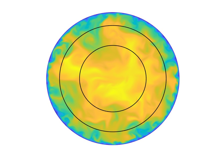
Since the early work by  Kim et al. (1987), direct numerical simulation (DNS) has become a widely used approach to study fundamental aspects of wall-bounded turbulence (Spalart & Watmuff, 1993; Hoyas & Jiménez, 2006; Sillero et al., 2013; Vinuesa et al., 2017; Pirozzoli et al., 2021; Alcántara-Ávila et al., 2021; Hoyas et al., 2022). Due to its profound implications, the overlap region of the mean velocity profile in wall-bounded turbulence has emerged as a focal point of considerable interest within the research community (See Figure 1). Here, the coexistence of large structures from the outer layer with smaller ones significantly affected by wall and viscous effects are observed (Townsend, 1976; Jiménez & Hoyas, 2008). Classical literature asserts that the mean velocity profile in this overlap region adheres to the renowned logarithmic law, characterized by its Kármán constant  (von Kármán, 1934; Millikan, 1938), $\kappa$. This formula reads:

$$\overline{U}_{x}^{+}(y^{+})=\frac{1}{\kappa}\log(y^{+})+B.$$ (1)

In this equation, $B$ is the interception constant, $\overline{U}_{x}$ is the mean streamwise velocity, and $y$ is the distance to the closest wall. All the quantities with $+$ superscripts have been nondimensionalized using the viscosity, $\nu$, and the friction velocity, $u_{\tau}$.

Figure 1: $r-\theta$ view of the instantaneous streamwise component $U_{x}$. The flow has been nondimensionalized by the maximum velocity. The scale goes from approximate $0$ (blue) to 1 (light yellow). The black lines indicate the boundaries of the overlap region, shown here at $y/\delta=0.2$ and $0.5$.

Figure 2: (Top) Streamwise velocity for the PHRF case (thick line), together with the pure log (dashed line) and log-plus-linear (thin line) overlap layers. (Bottom) Grid distance in the wall-normal direction, scaled with the Kolmogorov length. Colors as in Table 1, where solid lines denote pipe and dashed ones channel.

Over the years, this has been a topic of active study, and the universality of the log law and the von Kármán coefficient has occasionally been challenged or reaffirmed (George & Castillo, 2006; Barenblatt et al., 2000; Monkewitz et al., 2008; Vinuesa et al., 2014; Nagib & Chauhan, 2008; Luchini, 2017; Oberlack et al., 2022). Recently,  Monkewitz & Nagib (2023) (MN from now on) shed additional light on this topic, challenging the accumulated knowledge during the last century. MN’s main point is to consider in the inner asymptotic expansion a term proportional to the wall-normal coordinate, $\mathcal{O}(Re_{\tau}^{-1})$. Here $Re_{\tau}=u_{\tau}\delta/\nu$ is the friction Reynolds number with $\delta$ a characteristic outer length. This $\delta$ can be thought of as the radius $R$ in pipes, the semi-height in channels, $h$, or a length scale related to $\delta_{99}$ in boundary layers. Following MN, we find that the pure log law is not observed in channels and pipes (as well as other flows with streamwise pressure gradients) even if $Re_{\tau}$ is not above $\mathcal{O}(10^{4})$. MN’s extended matched asymptotics reveals an additional term in the expansion of the velocity for this layer, leading to an extra contribution in the overlap layer in the form $S_{0}y^{+}Re_{\tau}^{-1}$, where $S_{0}$ is a coefficient.

Figure 3: (Top) Intensities in the wall-normal and streamwise directions for all cases. (Bottom) $\overline{U}_{x}$. The inset shows the difference between the fine-resolution case and the others. Colors as in Table 1. Continuous lines, pipes and dotted lines, channels

Interestingly, the overlap region represented by a combined logarithmic and linear terms exhibits values of the von Kármán coefficient $\kappa$ consistent with those obtained from skin-friction relations, a fact that suggests that this approach can reveal high-$Re$ trends even at moderate Reynolds numbers. The main point of this matched asymptotic theory is to use a new expression in the overlap region for $\overline{U}_{x}$. MN’s formula reads:

$$\overline{U}_{x,\rm in}^{+}(y^{+}\gg 1)\sim\kappa^{-1}\ln y^{+}+B_{0}+B_{1}/Re_{\tau}+S_{0}y^{+}/Re_{\tau}.$$ (2)

Case	$Re_{\tau}$	$L_{x}/\delta$	$L_{z}/\delta$	$\Delta x^{+}$	$\Delta(R\theta^{+})$	$\max(\Delta y^{+}$)	$\min(\Delta y^{+})$	$N_{x}$	$N_{z}$	$N_{y}$	ETT	$\varepsilon$
PLRF	549	$10\pi$	$2\pi$	5.62	3	3.2	0.018	3072	1152	256	93	$1.2\times 10^{-4}$
PHRF	549	$10\pi$	$2\pi$	5.62	3	1.6	0.005	3072	1152	512	87	$2.6\times 10^{-4}$
PLRC	549	$10\pi$	$2\pi$	11.2	4.5	3.2	0.018	1536	768	256	184	$8.2\times 10^{-5}$
PHRC	549	$10\pi$	$2\pi$	11.2	4.5	1.6	0.005	1536	768	512	56	$3.8\times 10^{-4}$
CLRC	546	$8\pi$	$3\pi$	9	5	5.85	0.8	1536	1152	251	150	$7.6\times 10^{-5}$
CHRC	546	$8\pi$	$3\pi$	9	5	1.68	0.05	1536	1152	901	150	$3.8\times 10^{-5}$

Table 1: Summary of the simulations discussed in this work, where ‘P’ stands for pipe and ‘C’ for channel. The nomenclature ‘LR’ and ‘HR’ stands for low and high resolution in $y$, whereas ‘C’ and ´F’ denote coarse and fine in $x$ and $z$. Note that $L_{x}$ and $L_{z}$ are the periodic streamwise and spanwise dimensions while $h$ is the channel half height. $\Delta x^{+}$ and $\Delta z^{+}$ are the inner-scaled resolutions in terms of dealiased Fourier modes. The wall-normal direction is indicated in both flows by $y$. $N_{x},N_{z},$ and $N_{y}$ are the numbers of collocation points in the three different directions. The time span of the simulation is given in terms of eddy turnovers $u_{\tau}T/\delta$, and $\varepsilon$ is a measure of convergence, defined in Vinuesa et al. (2016). Colors given in the first column are used throughout the paper, while using dashed lines for the channel.

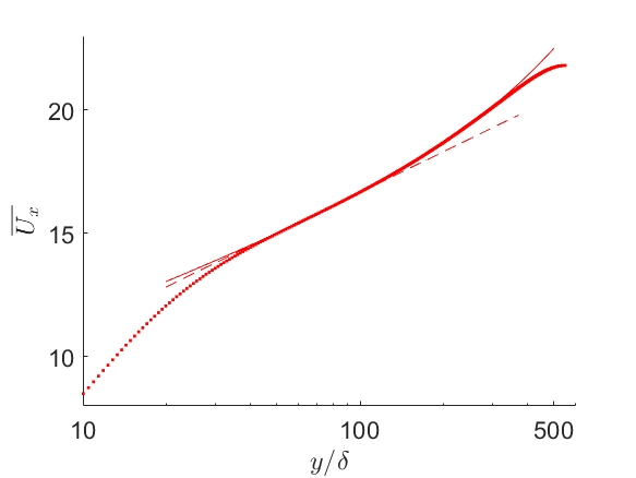
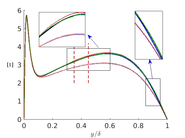
This model is depicted in Figure 2(top) as a thick line. The classic logarithmic is displayed using a thin line. However, to obtain accurate values of these coefficients, it is necessary to address two fundamental issues:

1. To find $\kappa$, the challenge is to identify the location and extent of the overlap region, which is weakly dependent on the Reynolds number (Monkewitz & Nagib, 2023).

2. To obtain the correct value of $S_{0}$, it is necessary to obtain with high accuracy the wall-normal distribution of ${\rm d\overline{U}_{x}^{+}}/{\rm d}y^{+}$.

Focusing on the second point above, it is possible to obtain an equation for the value of $\kappa$ and $S_{0}$ through the indicator function:

$$\Xi(y^{+})=y^{+}\frac{{\rm d}\overline{U}_{x}^{+}}{{\rm d}y^{+}}.$$ (3)

From equations (2) and (3), one can obtain the equation for $\kappa$ and $S_{0}$:

$$\Xi(y^{+})=\kappa^{-1}+S_{0}y^{+}/Re_{\tau}.$$

Thus, to accurately determine $S_{0}$, it is necessary to compute the indicator function with high accuracy, an aspect that has not been sufficiently investigated in the literature. While a convergence criterion exists for fully developed flows (Vinuesa et al., 2016), and the domain size of the problem has been examined in depth (Lozano-Durán & Jiménez, 2014; Lluesma-Rodríguez et al., 2018), the necessary grid spacing has received much less attention. Examples can be found in some very large simulations (Hoyas et al., 2022; Yao et al., 2023), where the authors only report their mesh size and compare their results with those in previous references, which basically do the same.

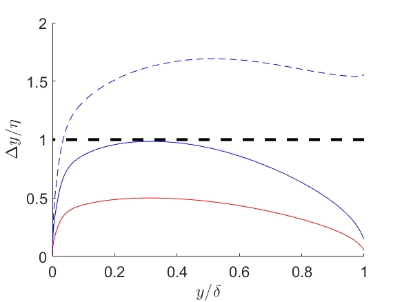
We have performed two different numerical experiments to examine this issue and its implications. The details can be found in Table 1. On the one hand, we have studied a smooth pipe of radius $R$ and length $L_{x}=10\pi R$ for $Re_{\tau}=550$. We will use $y$ to indicate the distance to the wall. We have used four different meshes, as seen in Table 1. The base mesh is the case PLRC with the same resolution in $x$ and $\theta$ as a channel. On the other hand, the mesh in the radial direction has twice the number of points needed in a channel due to the skewness of the cells near the pipe center. The mesh distribution can be seen in Figure 2 (bottom). Note that for the pipe cases, the wall-normal grid spacing is below the Kolmogorov scale throughout the computational domain. Starting with the PLRC, we doubled the cells in the radial direction (PHRC), azimuthal, and streamwise directions (PLRF), and all of them (PHRF). All these simulations ran for at least 55 eddy-turnover times (ETT), defined as ${\rm ETT}=Tu_{\tau}/R$. This is the primary motivation behind making our initial phase of DNS to $Re_{\tau}\sim 550$, as these cases can be run relatively quickly.

On the other hand, we have also run two channel-flow simulations. The first one (CLRC) is a simulation with the same mesh as Jiménez and Hoyas (Hoyas & Jiménez, 2008; Jiménez & Hoyas, 2008). The second one (CHRC) uses a mesh considered enough for $Re_{\tau}=3000$ (Lozano-Durán & Jiménez, 2014; Alcántara-Ávila et al., 2021). Two different codes were employed. OpenpipeFlow was used to run the pipe simulations (Willis, 2017; Yao et al., 2023). The code LISO was used for running the channel flow (Hoyas & Jiménez, 2006; Lluesma-Rodríguez et al., 2021; Yu et al., 2022). Both codes employ Fourier-decomposition techniques in the streamwise and spanwise directions. Openpipeflow uses a seventh-order finite-difference scheme in the wall-normal direction, while LISO uses a tenth-order compact-finite-difference scheme Lele (1992); Lluesma-Rodríguez et al. (2021).

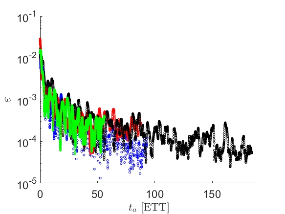
One of the tools used to assert whether a statistically steady state has been reached is to compute the total shear stress, as displayed in Figure 4. This equation is

$$1-y^{+}=\frac{\mathrm{d}\overline{U}_{x}^{+}}{\mathrm{d}{y}^{+}}-\overline{uv}^{+}.$$ (4)

where $\overline{uv}^{+}$ is the Reynolds stress. The parameter $\varepsilon$ is defined as the $L_{2}$ norm of the error between the left and right-hand sides of equation 4. As we can see, we do not obtain reasonable convergence until 50ETT, which is much longer than expected. It is clear that during the first 20 ETT, the simulation has a large statistical noise.

Figure 4: Evolution of the error in the momentum equation (4) integrated over the cross section, as a function of the averaging time $t_{a}$ expressed in eddy-turnover times.

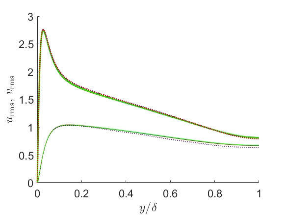
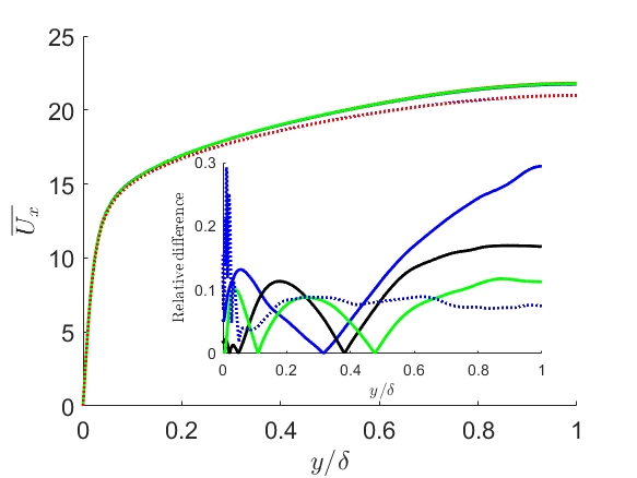
In the case of the pipe flow, the differences among the four simulations appear to be small when analyzing the streamwise and wall-normal fluctuations, as displayed in Figure 3 (top), and the streamwise velocity, Figure 3 (bottom). As shown in the latter, the difference between the coarser and finer cases is below $0.3\%$ everywhere. Such accuracy, however, is insufficient for utilizing the indicator function $\Xi$ to extract reliable coefficients of the overlap region. As shown in Figure 3 (bottom), the different curves of $\Xi$ do not collapse exactly in the region between $y/\delta=0.3$ and $y/\delta=0.5$, where the slope value of $\Xi$ is critical. This is more clearly appreciated in Figure 5 (Top), where the differences across cases can be more clearly assessed. Notice that the finer mesh, PHRF case, corresponds to the solid red line. The other three cases have not converged to the PHRF’s value even after 100 ETT. A better agreement is found in the case of the channels. Here, the convergence at $y/h=0.35$ is obtained after approximately 15 ETT. However, at $y/h=0.45$ the differences are of the order of 2% after 80 ETT, which is an extremely lengthy computation for high-Reynolds-number simulations.

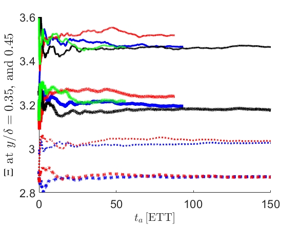
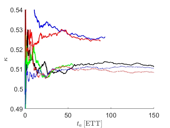
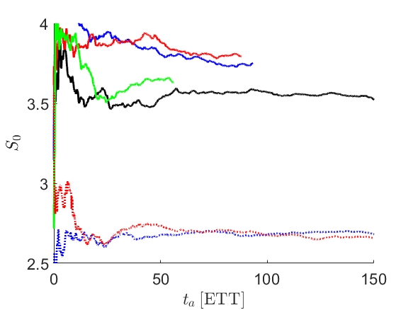
The effect of this lack of adequate resolution can be better evaluated by the time-averaged values of the overlap coefficients $\kappa$, $B$, and $S_{0}$ as functions of ETT. After 50 ETTs, the differences among the cases are still above 3$\%$, as shown in Figure 6. Again, the convergence for the channel case is better, but there remains a small difference up to ETT of 150, which corresponds to very expensive computations. In any case, at least 20 ETTs are needed to obtain a minimum level of convergence. Such differences in the indicator function $\Xi$ should be smaller for any reliable simulation to predict the values of $\kappa$, $B$, and $S_{0}$.

Finally, in the case of pipe flow, the values of these coefficients appear to depend on the azimuthal resolution, raising questions about the mesh aspect ratio of the grids. A careful study of such mesh variation effects in flows near their singularities, as in the case around the axis of pipes, is highly recommended. Such a study should also examine the sensitivity of the indicator function $\Xi$ to the order of the finite difference scheme used in the DNS. In general, the results demonstrate that classical and commonly used mesh sizes in the wall-normal direction for DNSs are not sufficiently fine to extract coefficients of the overlap region in wall-bounded turbulent flows, such as the von Kármán coefficient, $\kappa$.

Figure 5: (Top) $\Xi$ for the six case under study. (Bottom) Values of $\Xi$ at $y/\delta=0.35$ and $0.45$ as a function of the averaging time $t_{a}$ expressed in eddy-turnover times (ETT). Colors as in Table 1. Continuous lines for pipes, and dotted lines for channels. Thick lines represent, $y/\delta=0.35$, and thin ones, $y/\delta=0.45$.

Figure 6: $\kappa$ (top) and $S_{0}$ (bottom) for the six cases under study as functions of the averaging time $t_{a}$ expressed in ETT. Colors as in Table 1. Continuous lines for pipes, and dotted lines for channel

In conclusion, DNSs still stand as a powerful tool for exploring turbulent flows. However, the accuracy of DNS to compute certain important derivatives, such as those required for the indicator function $\Xi$ is challenged. To calculate $\Xi$, accurate values of the wall-normal derivative of the streamwise velocity must be established. This is a highly critical issue for experiments and should be addressed in all future measurements with more densely and equally spaced measurement locations in the wall-normal direction. Our investigation reveals that the indicator function exhibits sensitivity around the classic mesh size commonly used in DNSs. In particular, several coefficients of the overlap region required for Monkewitz and Nagib’s model of wall-bounded flows under streamwise pressure gradients cannot be found with less than 3% difference among the various meshes we tested. For example, this creates a new uncertainty source in estimating the von Kármán coefficient, which is very important for modeling and predicting wall-bounded turbulent flows. This uncertainty can also be generalized to any quantity needing wall-normal derivatives.

Data availability: The data used for this paper can be obtained by contacting S. Hoyas at serhocal@mot.upv.es.

References

- Alcántara-Ávila et al. (2021) Alcántara-Ávila, F., Hoyas, S. & Pérez-Quiles, M.J. 2021 Direct Numerical Simulation of thermal channel flow for and . Journal of Fluid Mechanics 916, A29.
- Barenblatt et al. (2000) Barenblatt, G. I., Chorin, A. J. & Prostokishin, V. M. 2000 A note on the intermediate region in turbulent boundary layers. Phys. Fluids 12, 2159–2161.
- George & Castillo (2006) George, W. K. & Castillo, L. 2006 Recent advancements toward the understanding of turbulent boundary layers. AIAA J. 44, 2435–2449.
- Hoyas & Jiménez (2006) Hoyas, S. & Jiménez, J. 2006 Scaling of the velocity fluctuations in turbulent channels up to . Phys. Fluids 18 (1), 011702.
- Hoyas & Jiménez (2008) Hoyas, S. & Jiménez, J. 2008 Reynolds number effects on the Reynolds-stress budgets in turbulent channels. Phys. Fluids 20 (10), 101511.
- Hoyas et al. (2022) Hoyas, S., Oberlack, M., Alcántara-Ávila, F., Kraheberger, S.V. & Laux, J. 2022 Wall turbulence at high friction reynolds numbers. Phys. Rev. Fluids 7, 014602.
- Jiménez & Hoyas (2008) Jiménez, J. & Hoyas, S. 2008 Turbulent fluctuations above the buffer layer of wall-bounded flows. J. Fluid Mech. 611, 215–236.
- von Kármán (1934) von Kármán, T. 1934 Turbulence and skin friction. J. Aero. Sci. 1, 1–20.
- Kim et al. (1987) Kim, J., Moin, P. & Moser, R. 1987 Turbulence statistics in fully developed channels flows at low Reynolds numbers. J. Fluid Mech. 177, 133–166.
- Lele (1992) Lele, S. K. 1992 Compact finite difference schemes with spectral-like resolution. Journal of Computational Physics 103 (1), 16–42.
- Lluesma-Rodríguez et al. (2018) Lluesma-Rodríguez, F., Hoyas, S. & Peréz-Quiles, MJ 2018 Influence of the computational domain on DNS of turbulent heat transfer up to for . International Journal of Heat and Mass Transfer 122, 983–992.
- Lluesma-Rodríguez et al. (2021) Lluesma-Rodríguez, F., Álcantara Ávila, F., Pérez-Quiles, M.J. & Hoyas, S. 2021 A code for simulating heat transfer in turbulent channel flow. Mathematics 9 (7).
- Lozano-Durán & Jiménez (2014) Lozano-Durán, A. & Jiménez, J. 2014 Effect of the computational domain on direct simulations of turbulent channels up to . Phys. Fluids 26 (1), 011702.
- Luchini (2017) Luchini, P. 2017 Universality of the turbulent velocity profile. Phys. Rev. Lett. 118, 224501.
- Millikan (1938) Millikan, C. M. 1938 A critical discussion of turbulent flows in channels and circular tubes. In Proc. 5th Int. Congr. Appl. Mech., Wiley, NY .
- Monkewitz & Nagib (2023) Monkewitz, P.A. & Nagib, H.M. 2023 The hunt for the kármán ‘constant’ revisited. Journal of Fluid Mechanics 967, A15.
- Monkewitz et al. (2008) Monkewitz, P. A., Chauhan, K. A. & Nagib, H. M. 2008 Comparison of mean flow similarity laws in zero pressure gradient turbulent boundary layers. Phys. Fluids 20, 105102.
- Nagib & Chauhan (2008) Nagib, H. M. & Chauhan, K. A. 2008 Variations of von kármán coefficient in canonical flows. Phys. Fluids 20, 101518.
- Oberlack et al. (2022) Oberlack, M., Hoyas, S., Kraheberger, S. V., Alcántara-Ávila, F. & Lawx, J. 2022 Turbulence statistics of arbitrary moments of wall-bounded shear flows: A symmetry approach. Phys. Rev. Lett. 128, 024502.
- Pirozzoli et al. (2021) Pirozzoli, S., Romero, J., Fatica, M., Verzicco, R. & Orlandi, P. 2021 One-point statistics for turbulent pipe flow up to . J. Fluid Mech. 926, A28.
- Sillero et al. (2013) Sillero, J.A., Jiménez, J. & Moser, R. D. 2013 One-point statistics for turbulent wall-bounded flows at reynolds numbers up to . Phys. Fluids 25, 105102.
- Spalart & Watmuff (1993) Spalart, P. R. & Watmuff, J. H. 1993 Experimental and numerical study of a turbulent boundary layer with pressure gradients. J. Fluid Mech. 249, 337–371.
- Townsend (1976) Townsend, A.A. 1976 The Structure of Turbulent Shear Flows, 2nd ed.. Cambridge University Press, New York,.
- Vinuesa et al. (2017) Vinuesa, R., Hosseini, S. M., Hanifi, A., Henningson, D. S. & Schlatter, P. 2017 Pressure-gradient turbulent boundary layers developing around a wing section 99, 613–641.
- Vinuesa et al. (2016) Vinuesa, R., Prus, C., Schlatter, P. & Nagib, H.M. 2016 Convergence of numerical simulations of turbulent wall-bounded flows and mean cross-flow structure of rectangular ducts. Meccanica 51 (12), 3025–3042.
- Vinuesa et al. (2014) Vinuesa, R., Schlatter, P. & Nagib, H. M. 2014 Role of data uncertainties in identifying the logarithmic region of turbulent boundary layers. Exp. Fluids 55, 1751.
- Willis (2017) Willis, Ashley P 2017 The Openpipeflow Navier–Stokes solver. SoftwareX 6, 124–127.
- Yao et al. (2023) Yao, J., Rezaeiravesh, S., Schlatter, P. & Hussain, F. 2023 Direct numerical simulations of turbulent pipe flow up to . Journal of Fluid Mechanics 956, A18.
- Yu et al. (2022) Yu, Linqi, Yousif, Mustafa Z, Zhang, Meng, Hoyas, Sergio, Vinuesa, Ricardo & Lim, Hee-Chang 2022 Three-dimensional esrgan for super-resolution reconstruction of turbulent flows with tricubic interpolation-based transfer learning. Phys. Fluids 34 (12).