Dark photon limits from patchy dark screening of the cosmic microwave background
Abstract
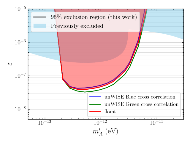
Dark photons that kinetically mix with the Standard Model photon give rise to new spectral anisotropies (patchy dark screening) in the cosmic microwave background (CMB) due to conversion of photons to dark photons within large-scale structure. We utilize predictions for this patchy dark screening signal to provide the tightest constraints to date on the dark photon kinetic mixing parameter ( (95% confidence level)) over the mass range eV, almost an order of magnitude stronger than previous limits, by applying state-of-the-art component separation techniques to the cross-correlation of Planck CMB and unWISE galaxy survey data.
Introduction — The cosmic microwave background (CMB) is an exquisitely well-calibrated source of photons. It has a near-perfect blackbody frequency spectrum and small ‘primary’ anisotropies (anisotropies imprinted on its release), consistent with Gaussian statistics. These properties can be used to isolate ‘secondary’ CMB anisotropies, induced by the interaction of CMB photons with large-scale structure (LSS) over cosmic history. For example, scattering from free electrons in LSS induces non-Gaussian and non-blackbody temperature and polarization anisotropies (Sunyaev-Zel’dovich, or SZ, effects Sunyaev and Zeldovich (1972, 1980)) that can be distinguished from the primary CMB. If the photon has interactions with particles beyond the Standard Model (BSM), the associated secondary CMB anisotropies provide a powerful discovery tool to search for new physics Pîrvu et al. (2024); Mondino et al. (2024).
One of the simplest extensions of the Standard Model is a light, massive vector boson Holdom (1986); Okun (1982), the dark photon (DP) , which can couple to the photon through kinetic mixing. The DP is motivated as a low-energy consequence of string theory Arvanitaki et al. (2010); Arias et al. (2012); Goodsell et al. (2009), a dark matter candidate Goodsell et al. (2009); Graham et al. (2016); East and Huang (2022), and a mediator of interactions with a larger dark sector (see Knapen et al. (2017) and references within). The mass range of interest for the DP spans many orders of magnitude, generating a diverse experimental program Pospelov et al. (2008); An et al. (2013); Baryakhtar et al. (2017, 2018); Barak et al. (2020); Hardy and Lasenby (2017); Lasenby and Van Tilburg (2021); Romanenko et al. (2023); Chaudhuri et al. (2015). For a DP with mass below eV, the signatures of interest are mainly cosmological and astrophysical Georgi et al. (1983); Mirizzi et al. (2009); Caputo et al. (2020a, b); Siemonsen et al. (2023); Siemonsen and East (2020).
As a consequence of kinetic mixing, CMB photons can convert to DPs as they propagate Georgi et al. (1983). The strongest, resonant, conversion occurs in regions where the photon plasma mass (proportional to the square root of the number density of electrons) is equal to the mass of the DP Mirizzi et al. (2009) — this is analogous to the Mikheyev-Smirnov-Wolfenstein (MSW) effect for neutrino oscillations in matter Wolfenstein (1978); Mikheyev and Smirnov (1985). Resonant conversion can occur due to the evolution of the cosmic mean density as the Universe expands Mirizzi et al. (2009) or due to the variation in density associated with the formation and evolution of LSS Caputo et al. (2020b, a). Measurements of the CMB monopole spectrum Fixsen et al. (1996) constrain the strength of the kinetic mixing Mirizzi et al. (2009); Caputo et al. (2020b, a). Ref. Pîrvu et al. (2024) demonstrated that these previous constraints could be greatly improved at DP masses by measuring the patchy screening of the CMB monopole, the frequency- and spatially-dependent reduction of intensity due to resonant conversion inside of non-linear structure. The characteristic spatial and spectral shape of the signal, as well as its correlation with tracers of LSS, can be used to separate the signal from the primary CMB and astrophysical foregrounds.111This framework can be extended to other BSM particles such as axions (e.g., Mondino et al. (2024); Mehta and Mukherjee (2024)).
In this Letter, we perform the first search for DPs via patchy dark screening of the CMB in cross-correlation with LSS, using data from the Planck mission Aghanim et al. (2020a) cross-correlated with the unWISE galaxy catalog Lang (2014); Meisner et al. (2017a, b); Schlafly et al. (2019); Krolewski et al. (2020) assembled from data taken by the Wide-field Infrared Survey Explorer (WISE) mission Wright et al. (2010); Mainzer et al. (2011). We place the strongest constraints to date on the strength of DP kinetic mixing in the mass range eV, improving existing constraints by almost an order of magnitude. Forecasts Pîrvu et al. (2024) suggest that even more dramatic improvements will be possible with data from future CMB Aguirre et al. (2019); Abazajian et al. (2019) and galaxy surveys Abell et al. (2009); Aghamousa et al. (2016); Doré et al. (2014).
Dark Photon Model — A kinetically mixed DP is described by the following Lagrangian222We use units where . Okun (1982); Holdom (1986):
| (1) |
where is the mass of the DP, is the kinetic mixing parameter, and ( is the photon (DP) field-strength tensor. The photon obtains a medium-dependent plasma mass , where is the free electron number density, and resonant conversion of CMB photons to DPs occurs at , when along any photon trajectory . The conversion probability can be computed via the Landau-Zener formula Mirizzi et al. (2009); Pîrvu et al. (2024), resulting in a position- and frequency-dependent (scaling as ) dark screening optical depth :
| (2) |
where the sum is over all resonances in the line of sight direction . The dark screening optical depth couples to the CMB monopole intensity , where is the Planck blackbody specific intensity at the CMB monopole temperature , resulting in a frequency-dependent specific intensity anisotropy , which can be extracted from multi-frequency CMB maps. In CMB thermodynamic temperature units, this takes the form where is the dimensionless photon frequency D’Amico and Kaloper (2015), with K Fixsen et al. (1996); Fixsen (2009).
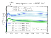
In Ref. Pîrvu et al. (2024), angular correlation functions of the dark screening map and of its cross-correlation with a template for the dark screening signal constructed from a tracer of LSS, , were computed within the halo model (see, e.g., Cooray and Sheth (2002) for a review). In the Supplemental Material (SM), we adapt this result to compute the cross-correlation , where the galaxy overdensity is modeled using the halo occupation distribution (HOD) described in Ref. Kusiak et al. (2022) for the unWISE galaxies. As in Ref. Pîrvu et al. (2024), we model the electron distribution in halos using the “AGN feedback” model of Ref. Battaglia (2016). We work with the harmonic transforms of the statistics, i.e., , where is the multipole moment.
Data and measurement: Dark screening map — The Planck satellite Aghanim et al. (2020a) mapped the full sky in nine microwave frequency bands. In our standard measurement, we use the sky maps produced by the NPIPE (PR4) data processing Akrami et al. (2020) at {30, 44, 70, 100, 143, 217, 353, 545} GHz. We apply several preprocessing steps to the maps, as described in Ref. McCarthy and Hill (2024a); in particular we mask and inpaint regions with bright point sources, as defined by the Planck point source masks, and a region near the Galactic center.
We use pyilc McCarthy and Hill (2024a)333https://github.com/jcolinhill/pyilc/ to construct a constrained needlet internal linear combination (NILC) Chen and Wright (2009); Remazeilles et al. (2011) map of the CMB spectral distortion induced by the DP conversion. NILC is a component separation technique that allows for minimum-variance estimation of the sky map of a component with a known frequency dependence (in this case, the DP distortion) via a linear combination of the frequency maps. In CMB thermodynamic temperature units, the frequency dependence of the DP distortion that we preserve is
| (3) |
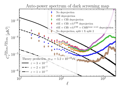
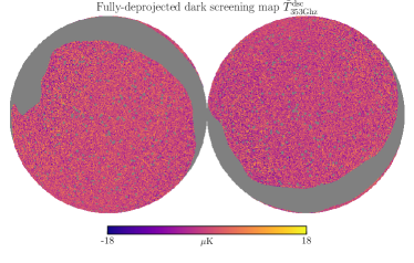
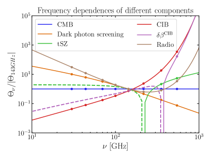
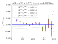
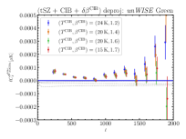
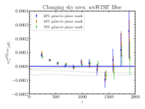
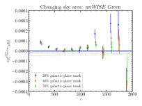
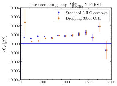
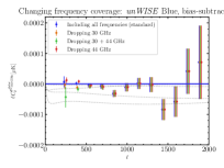
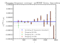
We normalize the DP distortion in Eq. (3) at 353 GHz, and thus we denote our NILC patchy dark screening map as . The angular power spectrum of the resulting map is plotted in Fig. 1 along with the predicted dark screening signal for several values of .
We choose constraints that allow us to directly remove, or ‘deproject,’ contamination from residual foregrounds in the NILC, in particular the thermal Sunyaev-Zel’dovich (tSZ) effect, the cosmic infrared background (CIB), and the blackbody CMB on large scales (which contains the integrated Sachs–Wolfe Sachs and Wolfe (1967) signal). These signals are correlated with the unWISE galaxies Kusiak et al. (2023, 2021); Ibitoye et al. (2022); Yan et al. (2024); Krolewski and Ferraro (2022), and as demonstrated in the SM, bias our measurement of the cross-correlation if not removed. The tSZ effect has a well-understood spectral dependence Sunyaev and Zeldovich (1970) and can therefore be deprojected exactly (as can the blackbody CMB). The spectral dependence of the CIB is less well-known, but we remove it by performing a Taylor expansion around an estimate of a model for its frequency dependence following Ref. Chluba et al. (2017); such a method was demonstrated to remove CIB contamination in an ILC setting in Refs. McCarthy and Hill (2024a, b).
We also construct two other versions of the undeprojected (standard ILC) map with independent noise realizations, from the independent half-ring splits of the NPIPE maps (these are co-added to produce the final NPIPE maps, such that each is twice as noisy as the final products). Their cross-power spectrum does not contain an instrumental noise term, so indicates the contribution from only foregrounds and signal.
As shown in Fig. 1, foreground deprojection comes at the expense of an increase in variance, since the NILC weights are constrained to explicitly remove the foregrounds rather than solely minimize the variance of the resulting map. This has the effect of weakening the sensitivity to dark screening, but increasing the robustness and interpretability of our results. We provide further details about the mapmaking procedure, including stability tests of the foreground removal, in the SM.
Data and measurement: LSS tracer (unWISE galaxies) — We cross-correlate our dark screening map with galaxy catalogs extracted from unWISE Lang (2014); Meisner et al. (2017a, b); Schlafly et al. (2019). We use both the “Blue” and “Green” unWISE samples described in Refs. Krolewski et al. (2020, 2021). These catalogs comprise objects from a broad range of redshifts, with the Blue sample at median redshift and the Green sample at . We convert the Green and Blue galaxy number density maps into overdensity maps by measuring the mean galaxy density and calculating
| (4) |
These catalogs have previously been used in various CMB cross-correlation analyses, including as a tracer of matter/galaxy overdensities for CMB lensing cross-correlations Krolewski et al. (2021); Farren et al. (2024, 2023) and of electron overdensities for kinetic SZ (kSZ) cross-correlations Kusiak et al. (2022); Coulton et al. (2024a); Kusiak et al. (2021); Bloch and Johnson (2024) and patchy Thomson screening cross-correlations Coulton et al. (2024a). In this work, we similarly use these maps to trace the electron distribution.
Cross-correlation measurement — We use pymaster Hivon et al. (2002); Alonso et al. (2019) to estimate the mask-decoupled cross-power spectrum between the NILC foreground-deprojected dark screening map and the unWISE maps. We apply the unWISE mask to the galaxies (retaining of the sky) and the union of the apodized preprocessing mask and the Planck Galactic plane mask to the dark screening map (retaining of the sky). The masks are described in the SM.
We measure power spectra in multipole bins of width , starting at . We do not use the largest-scale data point in our theoretical interpretation as it has a very large error bar (and is slightly unstable with respect to the choice of frequency coverage in the NILC). Our lowest multipole bin thus corresponds to .
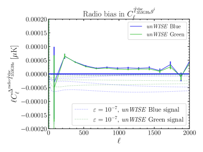
As described in greater detail in the SM, we find that our cross-correlation measurement is unstable to the removal of the lowest-frequency channels from the ILC, suggesting a residual extragalactic contribution from some other source in the NILC map. We expect that this is synchrotron emission from extragalactic radio sources, which we have not explicitly deprojected in the ILC.
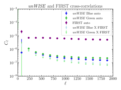
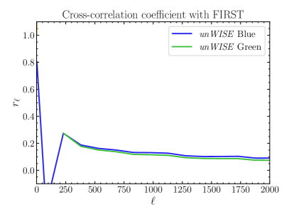
To assess the size of a possible radio bias, we directly measure the cross-correlation between our dark screening map and a catalog of radio-selected objects from the Very Large Array (VLA) Faint Images of the Radio Sky at Twenty centimeters (FIRST) survey White et al. (1997). The FIRST sources are detected via bright emission at 1.4 GHz, a much lower frequency than those used in our NILC map construction. We detect a correlation coefficient of between the FIRST sources and the unWISE samples. Additionally, the cross-correlation between our dark screening map and the FIRST catalog is positive and much higher than the cross-correlation between the dark screening map and the unWISE maps, indicating that there is some emission remaining in the NILC map that is more correlated with the radio sources than with unWISE. We build a template for the residual radio-unWISE signal as follows:
| (5) |
where is the measured cross-power spectrum of map with the FIRST map. This bias is small (equivalent in amplitude to a DP signal corresponding to in our most sensitive mass range, but with opposite sign). We describe this bias template in further detail in the SM. The bias can be measured for NILC maps constructed with different sets of frequency maps, and we find that upon subtraction of this bias the cross-correlation measurements become stable with respect to the choice of frequency coverage. We also validate our full pipeline, including the radio bias subtraction, with a signal injection test in the SM. Thus, in the following analysis we use the NILC map constructed from all eight Planck channels between 30 and 545 GHz, which yields the tightest constraints on and shows no evidence of additional bias.
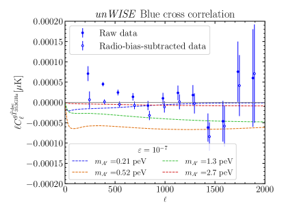
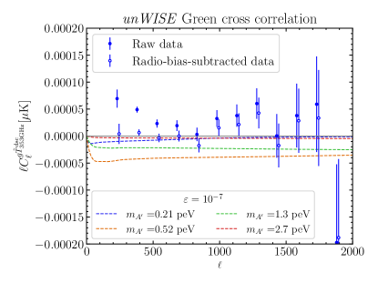
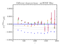
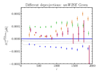
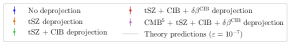
The measured cross-power spectra, before and after radio-bias subtraction, are shown in Fig. 2. We compute the mask-deconvolved covariance matrix for the cross-power spectrum assuming that the two maps are uncorrelated Gaussian random fields with underlying power spectra given by their measured power spectra Efstathiou (2006); Alonso et al. (2019). Note that, by comparison with Fig. 1, it is clear that the cross-correlation is a more sensitive probe of than the auto-power spectrum, confirming the forecasts of Ref. Pîrvu et al. (2024).
The with respect to null for each of the samples, including the 12 data points, with the radio bias subtracted, in the range we use for the separate analyses, are 17.71 for Blue; 9.85 for Green; and 26.80 for the combination (including their covariance). The associated probability-to-exceed (PTE) values are 0.12, 0.63, and 0.31, respectively, indicating consistency with a null detection.
Constraints on dark photon parameters — As is proportional to , we construct a Gaussian likelihood for :
| (6) | |||
where is the measured power spectrum data vector (with the radio bias subtracted) and is the theoretical model for this data vector (see the SM) for DP mass , with the index denoting either the Blue or Green unWISE sample. The covariance matrix is computed using pymaster to decouple the mask from the standard full-sky expression for uncorrelated Gaussian fields:
| (7) |
where and include all sources of signal and noise in the and fields respectively. In practice (and in particular in the absence of a model for all sources of noise and foregrounds in the field), we use the measured auto-power spectra in place of models to evaluate Eq. (7).
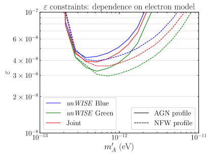
We scan over a range of in the region eV and compute . For each value, we adopt a uniform prior on over the domain . The DP mass to which our data are most sensitive is eV. The derived 95% confidence upper limits on as a function of are shown in Fig. 3. We find that for most of the covered mass range, almost an order-of-magnitude improvement compared to the previous best constraints in the literature.
For the purposes of these constraints, we hold fixed the parameters describing the electron distribution (to the AGN feedback model of Ref. Battaglia (2016)) and the galaxy HOD models. We demonstrate the validity of this approach in the SM.
Conclusion and Remarks — We have improved constraints on the kinetic mixing parameter of the DP in the mass range eV by almost an order of magnitude, using a foreground-cleaned cross-correlation between LSS tracers and the anisotropic dark screening induced by resonant conversion of CMB photons into DPs. This is the first time that such a CMB-LSS cross-correlation has been used to derive a constraint on light bosons in the dark sector, and demonstrates the power of such methods to constrain BSM physics.
Improvements in the analysis can be made with higher-sensitivity CMB experiments and deeper samples of LSS tracers. In addition, different DP masses can be probed by using LSS tracers that are sensitive to regions with different photon plasma mass, i.e., different electron densities. Theoretical calculations of such dark screening maps are underway. This method can also be adapted to search for patchy dark screening from axions Mondino et al. (2024); this is ongoing work.
We make our NILC dark screening maps public at https://users.flatironinstitute.org/~fmccarthy/dark_photon_screening_maps/.
Acknowledgements.—
We thank Gerrit Farren, Aleksandra Kusiak, and Cristina Mondino for useful discussions, and Alex Krolewski for providing us with the unWISE samples. This work made use of the healpy444https://healpy.readthedocs.io/en/latest/ library Zonca et al. (2019) (the Python implementation of HEALPix Górski et al. (2005)) as well as heavy use of numpy Harris et al. (2020).
We thank the Scientific Computing Core staff at the Flatiron Institute for computational support.
The Flatiron Institute is a division of the Simons Foundation. FMcC acknowledges support from the European Research Council (ERC) under the European Union’s Horizon 2020 research and innovation programme (Grant agreement No. 851274). MCJ and JH are supported by the Natural Sciences and Engineering Research Council of Canada through a Discovery grant. Research at Perimeter Institute is supported in part by the Government of Canada through the Department of Innovation, Science and Economic Development Canada and by the Province of Ontario through the Ministry of Research, Innovation and Science. JCH acknowledges support from NSF grant AST-2108536, NASA grant 80NSSC23K0463 (ADAP), NASA grant 80NSSC22K0721 (ATP), DOE HEP grant DE-SC0011941, the Sloan Foundation, and the Simons Foundation. The Dunlap Institute is funded through an endowment established by the David Dunlap family and the University of Toronto.
Note added: An analysis appeared on arXiv Aramburo-Garcia et al. (2024) during the final stage of this project, utilizing the temperature auto-correlation at 70 GHz to search for the patchy dark screening signal from dark photons. Our work improves on theirs both through the use of component separation and cross-correlation, an estimator shown to give stronger constraints than the auto-power spectrum in Ref. Pîrvu et al. (2024).
References
- Sunyaev and Zeldovich (1972) R. A. Sunyaev and Y. B. Zeldovich, Comments on Astrophysics and Space Physics 4, 173 (1972).
- Sunyaev and Zeldovich (1980) R. A. Sunyaev and Y. B. Zeldovich, MNRAS 190, 413 (1980).
- Pîrvu et al. (2024) D. Pîrvu, J. Huang, and M. C. Johnson, J. Cosmology Astropart. Phys 2024, 019 (2024).
- Mondino et al. (2024) C. Mondino, D. Pîrvu, J. Huang, and M. C. Johnson, arXiv e-prints (2024), 2405.08059 .
- Holdom (1986) B. Holdom, Phys. Lett. B 166, 196 (1986).
- Okun (1982) L. B. Okun, Sov. Phys. JETP 56, 502 (1982).
- Arvanitaki et al. (2010) A. Arvanitaki, S. Dimopoulos, S. Dubovsky, N. Kaloper, and J. March-Russell, Phys. Rev. D D81, 123530 (2010).
- Arias et al. (2012) P. Arias, D. Cadamuro, M. Goodsell, J. Jaeckel, J. Redondo, and A. Ringwald, J. Cosmology Astropart. Phys 06, 013 (2012).
- Goodsell et al. (2009) M. Goodsell, J. Jaeckel, J. Redondo, and A. Ringwald, J. High Energy Phys 11, 027 (2009).
- Graham et al. (2016) P. W. Graham, J. Mardon, and S. Rajendran, Phys. Rev. D 93, 103520 (2016).
- East and Huang (2022) W. E. East and J. Huang, J. High Energy Phys 12, 089 (2022).
- Knapen et al. (2017) S. Knapen, T. Lin, and K. M. Zurek, Phys. Rev. D 96, 115021 (2017).
- Pospelov et al. (2008) M. Pospelov, A. Ritz, and M. B. Voloshin, Phys. Rev. D 78, 115012 (2008).
- An et al. (2013) H. An, M. Pospelov, and J. Pradler, Phys. Rev. Lett. 111, 041302 (2013).
- Baryakhtar et al. (2017) M. Baryakhtar, R. Lasenby, and M. Teo, Phys. Rev. D D96, 035019 (2017).
- Baryakhtar et al. (2018) M. Baryakhtar, J. Huang, and R. Lasenby, Phys. Rev. D 98, 035006 (2018).
- Barak et al. (2020) L. Barak et al. (SENSEI), Phys. Rev. Lett. 125, 171802 (2020).
- Hardy and Lasenby (2017) E. Hardy and R. Lasenby, J. High Energy Phys 02, 033 (2017).
- Lasenby and Van Tilburg (2021) R. Lasenby and K. Van Tilburg, Phys. Rev. D 104, 023020 (2021).
- Romanenko et al. (2023) A. Romanenko et al., Phys. Rev. Lett. 130, 261801 (2023).
- Chaudhuri et al. (2015) S. Chaudhuri, P. W. Graham, K. Irwin, J. Mardon, S. Rajendran, and Y. Zhao, Phys. Rev. D 92, 075012 (2015).
- Georgi et al. (1983) H. Georgi, P. H. Ginsparg, and S. L. Glashow, Nature 306, 765 (1983).
- Mirizzi et al. (2009) A. Mirizzi, J. Redondo, and G. Sigl, J. Cosmology Astropart. Phys 03, 026 (2009).
- Caputo et al. (2020a) A. Caputo, H. Liu, S. Mishra-Sharma, and J. T. Ruderman, Phys. Rev. D 102, 103533 (2020a).
- Caputo et al. (2020b) A. Caputo, H. Liu, S. Mishra-Sharma, and J. T. Ruderman, Phys. Rev. Lett. 125, 221303 (2020b).
- Siemonsen et al. (2023) N. Siemonsen, C. Mondino, D. Egana-Ugrinovic, J. Huang, M. Baryakhtar, and W. E. East, Phys. Rev. D 107, 075025 (2023).
- Siemonsen and East (2020) N. Siemonsen and W. E. East, Phys. Rev. D 101, 024019 (2020).
- Wolfenstein (1978) L. Wolfenstein, Phys. Rev. D 17, 2369 (1978).
- Mikheyev and Smirnov (1985) S. P. Mikheyev and A. Y. Smirnov, Sov. J. Nucl. Phys. 42, 913 (1985).
- Fixsen et al. (1996) D. J. Fixsen, E. S. Cheng, J. M. Gales, J. C. Mather, R. A. Shafer, and E. L. Wright, ApJ 473, 576 (1996).
- Mehta and Mukherjee (2024) H. Mehta and S. Mukherjee, (2024), arXiv:2405.08879 [astro-ph.CO] .
- Aghanim et al. (2020a) N. Aghanim et al. (Planck collaboration), A&A 641, A1 (2020a).
- Lang (2014) D. Lang, AJ 147, 108 (2014).
- Meisner et al. (2017a) A. M. Meisner, D. Lang, and D. J. Schlegel, AJ 153, 38 (2017a).
- Meisner et al. (2017b) A. M. Meisner, D. Lang, and D. J. Schlegel, AJ 154, 161 (2017b).
- Schlafly et al. (2019) E. F. Schlafly, A. M. Meisner, and G. M. Green, ApJS 240, 30 (2019).
- Krolewski et al. (2020) A. Krolewski, S. Ferraro, E. F. Schlafly, and M. White, J. Cosmology Astropart. Phys 2020, 047 (2020).
- Wright et al. (2010) E. L. Wright et al., AJ 140, 1868 (2010).
- Mainzer et al. (2011) A. Mainzer et al., ApJ 731, 53 (2011).
- Aguirre et al. (2019) J. Aguirre et al. (Simons Observatory), J. Cosmology Astropart. Phys 1902, 056 (2019).
- Abazajian et al. (2019) K. Abazajian et al., (2019), arXiv:1907.04473 [astro-ph.IM] .
- Abell et al. (2009) P. A. Abell et al. (LSST collaboration), arXiv e-prints (2009), 0912.0201 .
- Aghamousa et al. (2016) A. Aghamousa et al. (DESI collaboration), arXiv e-prints (2016), 1611.00036 .
- Doré et al. (2014) O. Doré et al. (SPHEREx), arXiv e-prints (2014), 1412.4872 .
- D’Amico and Kaloper (2015) G. D’Amico and N. Kaloper, Phys. Rev. D 91, 085015 (2015), arXiv:1501.01642 [astro-ph.CO] .
- Fixsen (2009) D. J. Fixsen, ApJ 707, 916 (2009).
- Cooray and Sheth (2002) A. Cooray and R. Sheth, Phys. Rep. 372, 1 (2002).
- Kusiak et al. (2022) A. Kusiak, B. Bolliet, A. Krolewski, and J. C. Hill, Phys. Rev. D 106, 123517 (2022).
- Battaglia (2016) N. Battaglia, J. Cosmology Astropart. Phys 2016, 058 (2016).
- Akrami et al. (2020) Y. Akrami et al. (Planck collaboration), A&A 643, A42 (2020).
- McCarthy and Hill (2024a) F. McCarthy and J. C. Hill, Phys. Rev. D 109, 023528 (2024a).
- Chen and Wright (2009) X. Chen and E. L. Wright, ApJ 694, 222 (2009).
- Remazeilles et al. (2011) M. Remazeilles, J. Delabrouille, and J.-F. Cardoso, MNRAS 410, 2481 (2011).
- Sachs and Wolfe (1967) R. K. Sachs and A. M. Wolfe, ApJ 147, 73 (1967).
- Kusiak et al. (2023) A. Kusiak, K. M. Surrao, and J. C. Hill, Phys. Rev. D 108, 123501 (2023).
- Kusiak et al. (2021) A. Kusiak, B. Bolliet, S. Ferraro, J. C. Hill, and A. Krolewski, Phys. Rev. D 104, 043518 (2021).
- Ibitoye et al. (2022) A. Ibitoye, D. Tramonte, Y.-Z. Ma, and W.-M. Dai, ApJ 935, 18 (2022).
- Yan et al. (2024) Z. Yan, A. S. Maniyar, and L. van Waerbeke, J. Cosmology Astropart. Phys 05, 058 (2024).
- Krolewski and Ferraro (2022) A. Krolewski and S. Ferraro, J. Cosmology Astropart. Phys 04, 033 (2022).
- Sunyaev and Zeldovich (1970) R. A. Sunyaev and Y. B. Zeldovich, Ap&SS 7, 3 (1970).
- Chluba et al. (2017) J. Chluba, J. C. Hill, and M. H. Abitbol, MNRAS 472, 1195 (2017).
- McCarthy and Hill (2024b) F. McCarthy and J. C. Hill, Phys. Rev. D 109, 023529 (2024b).
- Krolewski et al. (2021) A. Krolewski, S. Ferraro, and M. White, J. Cosmology Astropart. Phys 2021, 028 (2021).
- Farren et al. (2024) G. S. Farren et al. (ACT collaboration), ApJ 966, 157 (2024).
- Farren et al. (2023) G. S. Farren, B. D. Sherwin, B. Bolliet, T. Namikawa, S. Ferraro, and A. Krolewski, arXiv e-prints (2023), 2311.04213 .
- Coulton et al. (2024a) W. R. Coulton et al. (ACT collaboration), arXiv e-prints (2024a), 2401.13033 .
- Bloch and Johnson (2024) R. Bloch and M. C. Johnson, arXiv e-prints (2024), 2405.00809 .
- Hivon et al. (2002) E. Hivon, K. M. Górski, C. B. Netterfield, B. P. Crill, S. Prunet, and F. Hansen, ApJ 567, 2 (2002).
- Alonso et al. (2019) D. Alonso, J. Sanchez, A. Slosar, and LSST Dark Energy Science Collaboration, MNRAS 484, 4127 (2019).
- White et al. (1997) R. L. White, R. H. Becker, D. J. Helfand, and M. D. Gregg, ApJ 475, 479 (1997).
- Efstathiou (2006) G. Efstathiou, MNRAS 370, 343 (2006).
- Zonca et al. (2019) A. Zonca, L. Singer, D. Lenz, M. Reinecke, C. Rosset, E. Hivon, and K. Gorski, Journal of Open Source Software 4, 1298 (2019).
- Górski et al. (2005) K. M. Górski, E. Hivon, A. J. Banday, B. D. Wandelt, F. K. Hansen, M. Reinecke, and M. Bartelmann, ApJ 622, 759 (2005).
- Harris et al. (2020) C. R. Harris et al., Nature 585, 357 (2020).
- Aramburo-Garcia et al. (2024) A. Aramburo-Garcia, K. Bondarenko, A. Boyarsky, P. Kashko, J. Pradler, A. Sokolenko, R. Kugel, M. Schaller, and J. Schaye, arXiv e-prints (2024), 2405.05104 .
- Peacock and Smith (2000) J. A. Peacock and R. E. Smith, MNRAS 318, 1144 (2000).
- Navarro et al. (1996) J. F. Navarro, C. S. Frenk, and S. D. M. White, ApJ 462 (1996), 10.1086/177173.
- Tinker et al. (2008) J. Tinker, A. V. Kravtsov, A. Klypin, K. Abazajian, M. Warren, G. Yepes, S. Gottlöber, and D. E. Holz, ApJ 688, 709 (2008).
- Tinker et al. (2010) J. L. Tinker, B. E. Robertson, A. V. Kravtsov, A. Klypin, M. S. Warren, G. Yepes, and S. Gottlöber, ApJ 724, 878 (2010).
- Bhattacharya et al. (2013) S. Bhattacharya, S. Habib, K. Heitmann, and A. Vikhlinin, ApJ 766, 32 (2013).
- Aghanim et al. (2020b) N. Aghanim et al. (Planck collaboration), A&A 641, A6 (2020b), [Erratum: Astron.Astrophys. 652, C4 (2021)].
- Narcowich et al. (2006) F. J. Narcowich, P. Petrushev, and J. D. Ward, SIAM Journal on Mathematical Analysis 38, 574 (2006).
- Bennett et al. (1992) C. L. Bennett et al., ApJ 396, L7 (1992).
- Bennett et al. (2003) C. L. Bennett et al., ApJS 148, 97 (2003).
- Page et al. (2007) L. Page et al., ApJS 170, 335 (2007).
- Delabrouille et al. (2009) J. Delabrouille, J. F. Cardoso, M. Le Jeune, M. Betoule, G. Fay, and F. Guilloux, A&A 493, 835 (2009).
- Hill and Spergel (2014) J. C. Hill and D. N. Spergel, J. Cosmology Astropart. Phys 2014, 030 (2014).
- Aghanim et al. (2016) N. Aghanim et al. (Planck collaboration), A&A 594, A22 (2016).
- Madhavacheril et al. (2020) M. S. Madhavacheril et al., Phys. Rev. D 102, 023534 (2020).
- Rotti et al. (2022) A. Rotti, A. Ravenni, and J. Chluba, MNRAS 515, 5847 (2022).
- Chandran et al. (2023) J. Chandran, M. Remazeilles, and R. B. Barreiro, MNRAS 526, 5682 (2023).
- Coulton et al. (2024b) W. R. Coulton et al. (ACT collaboration), Phys. Rev. D 109, 063530 (2024b).
- Ade et al. (2016) P. A. R. Ade et al. (Planck), Astron. Astrophys. 594, A4 (2016), arXiv:1502.01584 [astro-ph.CO] .
- Adam et al. (2016a) R. Adam et al. (Planck), Astron. Astrophys. 594, A7 (2016a), arXiv:1502.01586 [astro-ph.IM] .
- Zonca et al. (2009) A. Zonca et al., JINST 4, T12010 (2009), arXiv:1001.4589 [astro-ph.IM] .
- Ade et al. (2014) P. A. R. Ade et al. (Planck), Astron. Astrophys. 571, A9 (2014), arXiv:1303.5070 [astro-ph.IM] .
- Choi et al. (2020) S. K. Choi et al. (ACT), JCAP 12, 045 (2020), arXiv:2007.07289 [astro-ph.CO] .
- Adam et al. (2016b) R. Adam et al. (Planck collaboration), A&A 586, A133 (2016b).
- Stein et al. (2020) G. Stein, M. A. Alvarez, J. R. Bond, A. van Engelen, and N. Battaglia, J. Cosmology Astropart. Phys 2020, 012 (2020).
- Li et al. (2022) Z. Li, G. Puglisi, M. S. Madhavacheril, and M. A. Alvarez, J. Cosmology Astropart. Phys 2022, 029 (2022).
- Navarro et al. (1997) J. F. Navarro, C. S. Frenk, and S. D. M. White, ApJ 490, 493 (1997), arXiv:astro-ph/9611107 [astro-ph] .
- Amodeo et al. (2021) S. Amodeo et al., Phys. Rev. D 103, 063514 (2021), arXiv:2009.05558 [astro-ph.CO] .
- Schaan et al. (2021) E. Schaan et al., Phys. Rev. D 103, 063513 (2021), arXiv:2009.05557 [astro-ph.CO] .
Supplemental Material
Fiona McCarthy, Dalila Pîrvu, J. Colin Hill, Junwu Huang, Matthew C. Johnson, and Keir K. Rogers
This Supplemental Material contains supporting material for the main Letter, including details about the signal modeling and needlet ILC mapmaking, as well as discussions about the impact of deprojection choices, frequency coverage, sky area, and masks.
I Signal Modeling
In this work we use the same assumptions to model the DP-induced spectral distortion anisotropies as in Ref. Pîrvu et al. (2024). We extend the analysis of this work to include the cross-correlation between the dark screening optical depth and the halo occupation distributions (HODs) Peacock and Smith (2000) representing the unWISE Blue and Green galaxy catalogs. A similar calculation is performed in Mondino et al. (2024) for the case of axion-induced dark screening.
The optical depth for photon-dark photon conversion is the sum over all resonance events that take place along each line of sight , as defined in Eq. (2). Within the halo model, this quantity can be factorized into contributions from each halo , which can be described by the product of an isotropic and an anisotropic term:
| (S1) |
where we have defined
| (S2) |
Note that we assume that these quantities are functions of halo mass and redshift only, and is comoving distance to . Above, is the halo-centric radius at which the resonance condition is met and the virial radius is taken as the halo boundary, beyond which no conversion takes place. The angle between the halo center and the photon arrival direction is defined as , such that . The function counts the number of resonance crossings per halo; it equals when , since the photon crosses the resonance once as it enters the halo and a second time exiting the halo, and is set to 1 when the photon grazes the resonance surface at . Finally, is the radial profile of the ionized gas density within a spherically symmetric halo. We adopt the “AGN feedback” profile from Ref. Battaglia (2016), which is obtained from hydrodynamical cosmological simulations, and is defined in detail in Ref. Pîrvu et al. (2024).
Taking the ensemble average over the halos distributed along the line of sight and performing a harmonic transform, we arrive at the expression for the DP optical depth:
| (S3) |
where is the Legendre polynomial of degree . The DP-induced fluctuation in the CMB temperature is
| (S4) |
where and K is the CMB monopole temperature.
The cross-power spectrum between a patchy dark screening map and a galaxy number density map is formally obtained by taking the product of the multipole-space kernels of the dark screening-induced temperature fluctuations and a galaxy overdensity field , weighted by the halo mass function , defined as the isotropic average halo number density per comoving volume element and halo mass. Within the halo model framework, the cross-correlation is defined as a sum of a 1-halo term, which carries the small-scale dependence on the halo density profile’s projected angular shape, and a 2-halo term, proportional to the clustering of halos:
| (S5) | ||||
where is the Hubble rate at , is the linear matter power spectrum evaluated at redshift and comoving wavenumber , and is the linear halo bias.
To model how the observed galaxies populate the underlying dark matter halo distribution, we use the HOD described in Ref. Kusiak et al. (2022). The galaxy multipole space kernel is given by:
| (S6) |
where
| (S7) |
and the functions and represent the expectation values for the number of central and satellite galaxies respectively. These functions are parametrized as a function of halo mass as:
| (S8) |
Eq. (S6) above defines central galaxies as lying at the center of each halo, while satellites are distributed according to an NFW profile, where is the normalized harmonic transform of the NFW density profile Navarro et al. (1996), truncated at . Finally, the quantity is the redshift distribution of the empirical galaxy sample, normalized to unity. Overall, this HOD model is defined by five free parameters: . The HOD values used in this work are the best-fit set of parameters obtained for the unWISE Blue and Green samples in Ref. Kusiak et al. (2022).
For the numerical modeling of the template signal we use a modified version of the code hmvec.555https://github.com/simonsobs/hmvec We assume that within the virial radius, the halo density is 178 times the critical density of the universe, i.e., . We use the halo mass function of Ref. Tinker et al. (2008) that fixes the halo bias function Tinker et al. (2010), as well as the concentration-mass relation from Ref. Bhattacharya et al. (2013). To evaluate the integrals, we use equal redshift bins in the range and logarithmically-spaced halo mass bins . We assume a flat CDM cosmology, with parameters from the best-fit Planck model Aghanim et al. (2020b): , , , , .
II NILC mapmaking
In CMB thermodynamic temperature units, the frequency dependence of the DP-induced spectral distortion is
| (S9) | ||||
| (S10) |
where is the kinetic mixing parameter (see Eq. (1)), K is the CMB monopole temperature, and is the redshift-independent dimensionless photon frequency. We normalize this distortion at a reference frequency of 353 GHz, and thus we denote our NILC reconstruction of this distortion as . The ILC estimate is a linear combination of frequency maps that preserves the spectral energy distribution (SED) of a signal of interest — in our case, that in Eq. (S10) — while minimizing the variance of the estimated map, given the frequency-frequency covariance matrix, which is estimated directly from the data. For NILC, the covariance matrix is estimated on a needlet frame Narcowich et al. (2006), allowing for simultaneous harmonic (angular)-space and pixel-space localization. ILC has a long history of applications to CMB data (e.g., Bennett et al. (1992, 2003); Page et al. (2007); Delabrouille et al. (2009); Hill and Spergel (2014); Aghanim et al. (2016); Madhavacheril et al. (2020); Rotti et al. (2022); Chandran et al. (2023); McCarthy and Hill (2024a); Coulton et al. (2024b)) to isolate components with well-understood SEDs such as the blackbody CMB temperature anisotropy and the Compton- distortion induced by the thermal SZ (tSZ) effect Sunyaev and Zeldovich (1970). We use a constrained ILC Chen and Wright (2009); Remazeilles et al. (2011) to deproject the SEDs of other sky components that could bias our measurement — in particular, the tSZ SED; a modified blackbody SED with spectral index and temperature K; and the first derivative of this modified blackbody with respect to . The latter two constraints effectively remove the cosmic infrared background (CIB) signal, following the moment expansion approach of Ref. Chluba et al. (2017). Lastly, on large scales (the first five of the harmonic needlet scales defined below) we deproject a blackbody SED with temperature K Fixsen et al. (1996); Fixsen (2009) to remove the blackbody CMB anisotropies, which are correlated on large scales with the galaxy overdensity field due to the late-Universe integrated Sachs-Wolfe (ISW) effect Sachs and Wolfe (1967).
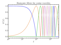
We use cosine needlets in our NILC, which have the following harmonic filters:
| (S11) |
We use 13 harmonic needlet scales with the values given by {0, 100, 200, 300, 400, 600, 800, 1000, 1250, 1400, 1800, 2200, 4097} (following Ref. Coulton et al. (2024b)). The harmonic needlet filters are shown in Fig. S1.
The calculation of the covariance matrix from the data leads to the well-known “ILC bias” Delabrouille et al. (2009), where chance fluctuations in the noise can be used to artificially minimize the variance of the inferred signal. This bias can be controlled by measuring the covariance matrix from regions which contain a large enough number of modes. In particular, by using Gaussian real-space kernels with standard deviation given by McCarthy and Hill (2024a)
| (S12) |
where is the number of components deprojected and is the number of frequency channels used in the ILC, we maintain a fractional ILC bias less than . Our real-space filters are Gaussian, with FWHMs chosen at each scale to ensure that the fractional ILC bias is 0.01 for an undeprojected map with full frequency coverage. We drop frequency channels when their beam functions become smaller than a certain threshold depending on the needlet filters; the frequency channels included, as well as the real-space filter sizes, at each needlet scale are given in Table S1. Note that we treat the Planck beams Ade et al. (2016); Adam et al. (2016a) as isotropic Gaussians, as described in Ref. McCarthy and Hill (2024a).
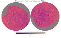
We construct all of our NILC dark screening maps at a reference frequency of 353 GHz. The auto-power spectra of our maps are shown in Fig. 1. The maps themselves are shown in Fig. S2.
| Harmonic scale | Frequencies included | Real-space filter FWHM (degrees) | |
|---|---|---|---|
| 0 | 0 | 30,44,70,100,143,217,353,545 GHz | 91.8 |
| 1 | 100 | 30,44,70,100,143,217,353,545 GHz | 35.6 |
| 2 | 200 | 30,44,70,100,143,217,353,545 GHz | 25.2 |
| 3 | 300 | 30,44,70,100,143,217,353,545 GHz | 20.6 |
| 4 | 400 | 30,44,70,100,143,217,353,545 GHz | 14.1 |
| 5 | 600 | 30,44,70,100,143,217,353,545 GHz | 10.3 |
| 6 | 800 | 44,70,100,143,217,353,545 GHz | 8.26 |
| 7 | 1000 | 70,100,143,217,353,545 GHz | 6.31 |
| 8 | 1250 | 70,100,143,217,353,545 GHz | 6.11 |
| 9 | 1400 | 70,100,143,217,353,545 GHz | 4.74 |
| 10 | 1800 | 70,100,143,217,353,545 GHz | 3.55 |
| 11 | 2200 | 143,217,353,545 GHz | 1.34 |
| 12 | 4097 | 143,217,353,545 GHz | 1.28 |

The frequency scalings of various components of interest for the problem are shown in Fig. S3. To compute the signal due to each component in a given Planck frequency map, we integrate these SEDs over the Planck passbands Zonca et al. (2009); Ade et al. (2014), as described in Ref. McCarthy and Hill (2024a).
III Impact of deprojection choices and CIB model
We measure using a map that has the tSZ spectral distortion, the CIB, and the first moment of the CIB with respect to deprojected, along with the primary CMB blackbody on large scales (in particular, the first five harmonic needlet scales, so ). In this section, we show the impact of these deprojections and demonstrate the insensitivity of our measurements to the assumed frequency dependence of the CIB SED.
In Fig. S4 we show the impact of the deprojection choices in the NILC map on the final measurement. A striking feature of this plot is the necessity for tSZ deprojection. If an unconstrained (pure minimum-variance) ILC is used, the residual tSZ foreground is significant enough to bias the measurement very high.
In Fig. S5 we demonstrate the stability of the measurement with respect to the choices of the parameters used to deproject the CIB. In particular, the CIB SED is modeled as a modified blackbody at temperature and with spectral index :
| (S13) |
where is the Planck function. The parameters and are uncertain and indeed different for each object that comprises the CIB. On average, however, the appropriate , may depend on the mean redshift of the objects one is interested in. In particular, Ref. McCarthy and Hill (2024a) found that the CIB monopole (as predicted by the CIB model constrained by the Planck CIB auto-power spectrum in Ref. Adam et al. (2016b)) is best fit by . However, the CIB monopole is sourced at higher redshift than the anisotropies we are interested in, and so the appropriate temperature is likely higher than this (the CIB temperature increases with redshift, but does so slower than , the factor that describes the redshift of the photons, so the effective temperature decreases with redshift).
In any case, it is clear from Fig. S5 that the deprojection with respect to CIB is insensitive to the choice of CIB SED, within a reasonable range, indicating that we have removed the systematics due to residual CIB contamination in the cross-correlation measurement. Without the additional moment deprojection (referred to as deprojection), the measurement is strongly dependent on the choice of parameters.

IV Sky area and masks
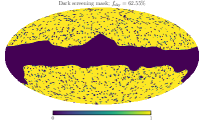
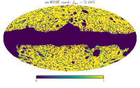
Our measurement is made with the dark screening map masked by the union of the preprocessing mask and the Planck 70% Galactic plane mask (the mask that leaves 70% of the sky unmasked), apodized with a scale of 30 arcminutes using the “C2” apodization routine of namaster. The unWISE galaxies are masked by the unWISE mask, which is the union of a point source mask and the Planck CMB lensing mask. Following Ref. Kusiak et al. (2021), we apodize only the Planck CMB lensing contribution to this mask, with an apodization scale of 60 arcminutes, again using the “C2” routine of namaster. These masks are shown in Fig. S6, and the dark screening maps themselves (for various deprojection choices) are shown in Fig. S2.
In Fig. S7 we show the cross-correlation measurements as we vary the amount of the Galactic plane that we mask, to test for Galactic contamination in our data. Generally, there is no evidence of such contamination, as the measurements are all broadly consistent.
V Radio bias subtraction
As we have not explicitly deprojected foreground contamination due to radio sources in the NILC dark screening map, the possibility of a residual extragalactic radio contribution that is correlated with the unWISE galaxies remains.666Note that the NILC procedure will naturally clean a significant amount of radio contamination via its variance-minimization objective. To assess the level of bias from this contribution, we directly measure the cross-correlation of the unWISE galaxy samples with a separate radio galaxy catalog from the FIRST survey White et al. (1997). We measure the cross-correlation on the area of sky left unmasked by the union of the unWISE mask and the mask removing the sky area not covered by FIRST. The unWISE Green and Blue samples have a correlation with the FIRST catalog, as shown in Fig. S8. The correlation coefficient between fields and is estimated as
| (S14) |
The cross-correlation between our fully-deprojected dark screening map and the FIRST catalog is shown in Fig. S9. There is a clear non-zero positive correlation, a sign of residual positive radio emission in the dark screening map. Additionally, the measurement depends on the frequency coverage of the map (see below), a sign that we are detecting something with a different SED to the DP signal.
Note that radio sources are brightest at low frequencies, and would be expected to leak into the measurement as a positive (emission) signal, due to the relatively similar shape of the synchrotron SED and the DP distortion SED that our NILC preserves. Indeed, we verify with simulations that this is the case — in particular, we perform our NILC procedure on the Planck mm-wave sky simulations described in Ref. McCarthy and Hill (2024b), which include extragalactic signals from the Websky simulations Stein et al. (2020), including a radio component that is correlated with LSS Li et al. (2022). In the absence of a proper unWISE mock galaxy catalog built from the Websky matter density field, we correlate our NILC dark screening map (constructed from the Websky frequency maps) with the Websky halo catalog, reweighted to have the same redshift distribution as the unWISE Blue galaxy catalog (as well as the Websky CMB lensing convergence map, which is sourced at higher redshift than the unWISE galaxies), and verify that the radio bias is positive.
Under the assumption that this measurement is dominated by the radio residuals in the dark screening map correlating with the FIRST catalog, we can use it to create a model of the residual radio – unWISE correlation. Specifically, writing the dark screening map as
| (S15) |
where are the remaining uncorrelated foregrounds and noise, is the true dark screening signal, and is the radio residual, we have
| (S16) |
In the unWISE – DP cross-correlation, we have
| (S17) |
we can thus use the FIRST measurements to estimate
| (S18) |
We show these bias estimates explicitly in the right panel of Fig. S9. They have a similar scale dependence to the expected dark screening signal, with a magnitude corresponding to for the masses that our data are most sensitive to (but with opposite sign, as they are due to emission rather than screening).
VI Frequency coverage
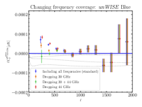
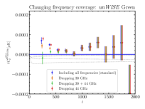
In our nominal results, we include the {30, 44, 70, 100, 143, 217, 353, 545} GHz Planck intensity maps. In the top of Fig. S10, we show the cross-correlation measurements when the lower-frequency channels, 30 and 44 GHz, are excluded from the construction of the NILC dark screening map.
When all frequency channels are included, before radio-bias subtraction a positive (emission) signal is evident at low (). This residual bias is removed when we drop the lowest-frequency channels (30 and 44 GHz) from the measurement, and is generally stable to the additional removal of the 70 GHz channel (not shown in the plots).
This instability to the choice of frequency coverage is evidence for a frequency-dependent residual foreground in the NILC map, which we attribute to radio emission (see above). However, after performing the radio-bias subtraction described in the previous section (with the radio bias recalibrated for each choice of frequency coverage), we note that this procedure brings the data into agreement for all choices of frequency coverage, as shown in the bottom of Fig. S10.
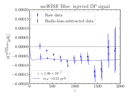
VII Recovery of an artificial signal
To ensure that our pipeline is unbiased, we inject an artificial signal into the data and demonstrate that we can recover it. We create the artificial signal by first filtering the unWISE map to create a map with the appropriate correlation:
| (S19) |
where is our signal prediction and is the measured unWISE Blue auto-power spectrum, which is effectively noiseless over the range of scales considered here due to its extremely low shot noise (i.e., high number density). We choose a signal corresponding to and . We add this to the Planck single-frequency maps with the appropriate DP-distortion frequency dependence and then perform NILC component separation.
We measure the cross-correlation of this signal-injected NILC map with the unWISE Blue sample, and we re-calibrate the radio bias from this map using the FIRST data as described above. This is very important, as we aim to explicitly verify that the radio bias subtraction step does not artificially subtract the true signal.
The recovery of the input signal is demonstrated in Fig. S11, thereby validating our pipeline, including the radio bias subtraction. The between the data and the model curve is 15.58 for 12 points, which corresponds to a PTE of 0.21, indicating good agreement.
VIII Changes to the galaxy and electron models
In our nominal analysis, we hold fixed the astrophysical quantities appearing in the halo model used to compute , as described in SM I. In reality, there is some uncertainty associated with both the galaxy HOD and electron density profile models. Properly, one should marginalize over these uncertainties, e.g., by performing a full Markov Chain Monte Carlo (MCMC) analysis with the HOD and electron profile parameters allowed to vary. However, such an operation would be computationally expensive and, as we show below, unlikely to significantly change our derived constraints on . In this section, we explore the dependence of our DP constraints on such changes to the underlying astrophysical modeling assumptions, to justify our decision to ignore the associated marginalization.
VIII.1 Uncertainties in the galaxy HOD model
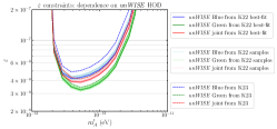
The unWISE HOD parameters we use were obtained in Ref. Kusiak et al. (2022) from fits to galaxy clustering and galaxy – CMB lensing cross-correlation data. To explore the uncertainty involved in these fits, we draw 20 samples from the MCMC chains used to approximate the posterior distributions in Ref. Kusiak et al. (2022); these can be thought of as a prior on the galaxy HOD model. We then re-run our analysis pipeline to obtain constraints on for each set of galaxy HOD parameters. We show in Fig. S12 the distribution of the constraints we obtain when we vary the HOD model in this way. In general, the results obtained with the best-fit HOD model were representative; the constraints degrade at most from at their strongest to , a degradation of only 5%.
A larger, but not significant, degradation in the constraints is found when we switch from the best-fit model of Ref. Kusiak et al. (2022) (K22) to that of Ref. Kusiak et al. (2023) (K23) (see their Appendix B). In K23, the HOD parameters were fit to data at higher than in K22 (where only the large scales, , were used). In particular, due to the change in the best-fit value of the parameter from 0.687 to 0.02, the prediction of is much lower in the K23 model. These changes in the predictions for are explicitly shown in the right panel of Fig. S12.
VIII.2 Uncertainties in the electron model
There are also uncertainties in the electron density profile model used in the computation of . In our nominal analysis, we use the spherically-symmetric generalized Navarro-Frenk-White (gNFW) profiles fit in Ref. Battaglia (2016) to hydrodynamic simulations incorporating feedback from active galactic nuclei (AGNs). Responding to the feedback, the electrons are distributed more smoothly than the dark matter, which follows the standard NFW profile Navarro et al. (1997). To indicate how our constraints on could change due to different assumptions about the electron distribution, we calculate assuming that the electrons exactly trace the dark matter; this is an extreme assumption that is empirically ruled out Amodeo et al. (2021); Coulton et al. (2024a). The resulting constraints are shown in Fig. S13.
We see that the inclusion of AGN feedback (and the other non-gravitational physics included in the simulations of Ref. Battaglia (2016)) reduces our sensitivity to at the high end of the relevant DP mass range. Thus, if AGN feedback is weaker than that in the simulations on which these profiles are based, our constraints are conservative. Updated DP analyses using new electron density profile modeling constraints, such as from kinematic SZ measurements Amodeo et al. (2021); Schaan et al. (2021); Kusiak et al. (2021) would be interesting.