To Believe or Not to Believe Your LLM

Abstract

We explore uncertainty quantification in large language models (LLMs), with the goal to identify when uncertainty in responses given a query is large. We simultaneously consider both epistemic and aleatoric uncertainties, where the former comes from the lack of knowledge about the ground truth (such as about facts or the language), and the latter comes from irreducible randomness (such as multiple possible answers). In particular, we derive an information-theoretic metric that allows to reliably detect when only epistemic uncertainty is large, in which case the output of the model is unreliable. This condition can be computed based solely on the output of the model obtained simply by some special iterative prompting based on the previous responses. Such quantification, for instance, allows to detect hallucinations (cases when epistemic uncertainty is high) in both single- and multi-answer responses. This is in contrast to many standard uncertainty quantification strategies (such as thresholding the log-likelihood of a response) where hallucinations in the multi-answer case cannot be detected. We conduct a series of experiments which demonstrate the advantage of our formulation. Further, our investigations shed some light on how the probabilities assigned to a given output by an LLM can be amplified by iterative prompting, which might be of independent interest.

1 Introduction

Who’s talking? I asked, peering behind the mirror. Many dead spiders and a lot of dust were there. Then I pressed my left eye with my index finger. This was an old formula for detecting hallucinations, which I had read in To Believe or Not to Believe?, the gripping book by B. B. Bittner. It is sufficient to press on the eyeball, and all the real objects, in contradistinction to the hallucinated, will double. The mirror promptly divided into two and my worried and sleep-dulled face appeared in it.

—"Monday Starts on Saturday" by A. and B. Strugatsky

Like the protagonist of the novel, language models too occasionally suffer from hallucinations, or responses with low truthfulness, that do not match our own common or textbook knowledge (Bubeck et al., 2023, Gemini Team, Google, 2023). At the same time, since LLMs work by modeling a probability distribution over texts, it is natural to view the problem of truthfulness through the lens of statistical uncertainty. In this paper we explore uncertainty quantification in LLMs. We distinguish between two sources of uncertainty: epistemic and aleatoric (Wen et al., 2022, Osband et al., 2023, Johnson et al., 2024). Epistemic uncertainty arises from the lack of knowledge about the ground truth (e.g., facts or grammar in the language), stemming from various reasons such as insufficient amount of training data or model capacity. Aleatoric uncertainty comes from irreducible randomness in the prediction problem, such as multiple valid answers to the same query. Hence, truthfulness can be directly analyzed via looking at the epistemic uncertainty of a model in the sense that when the epistemic uncertainty is low, the model predictions must be close to the ground truth.

Rigorously identifying when (either) uncertainty is small is notoriously hard, especially in deep neural networks (Blundell et al., 2015, Antorán et al., 2020). This is because we generally lack guarantees about learning the ground truth (consistency), or even a weaker guarantee about how large the variance of a learning algorithm is. At the same time, there exist many heuristic approaches for uncertainty quantification based on simply looking at the log-likelihood of responses (Kadavath et al., 2022), estimating entropy (Kuhn et al., 2023), ensembling (Lakshminarayanan et al., 2017b, Dwaracherla et al., 2023, Osband et al., 2023), or sometimes even more principled formulations, such as conformal prediction (Angelopoulos et al., 2023, Ravfogel et al., 2023, Yadkori et al., 2024) (which however come with strong assumptions).

To the best of our knowledge, a common limitation of these approaches is that they are only meaningful in problems where there exists a single correct response (e.g. label) as they aim for detecting if one response is dominant (or multiple responses with the same meaning), that is, if there is only little uncertainty in the prediction. On the other hand, when multiple responses are correct, that is, there is aleatoric uncertainty in the ground truth, simply estimating the amount of uncertainty in the LLM’s output is insufficient, as the perfect (ground-truth) predictor may have large aleatoric uncertainty and no epistemic uncertainty, while a completely useless predictor may have large epistemic uncertainty only, but the total amount of uncertainty of the two predictors might be the same.

Contributions.

In this paper we address the above problem directly, and design methods to decouple epistemic and aleatoric uncertainty, allowing us to effectively deal with multi-response queries. Rather than trying to quantify how small epistemic uncertainty can be, we aim to identify when only the epistemic uncertainty is large, in which case we can suspect that the response is hallucinated.

As a starting point we make a simple observation: If multiple responses are obtained to the same query from the ground truth (the language), they should be independent from each other, that is, in probabilistic interpretation, the joint distribution of these multiple responses, for a fixed query, must be a product distribution.

This observation can be used to measure how far the language model can be from the ground truth. The sequential model implemented by a language model allows us to construct a joint distribution over multiple responses, which is done through iterative prompting of an LLM based on its previous responses and the application of the chain rule of probability: first we ask the model to provide a response given a query, then to provide another response given the query and the first response, then a third one given the query and the first two responses, an so on. This is in contrast to some of the earlier works that approached decoupling epistemic and aleatoric uncertainty for classification problems by training the model with pairs (or tuples) of labels (Wen et al., 2022).

So, if the response to a prompt containing the query and previous responses is insensitive to the previous responses, we have the desired independence and the LLM-derived joint distribution can be arbitrarily close to the ground truth. On the other hand, if the responses within the context heavily influence new responses from the model then, intuitively speaking, the LLM has low confidence about the knowledge stored in its parameters, and so the LLM-derived joint distribution cannot be close to the ground truth. As more responses are added to the prompt, this dependence can be made more apparent, allowing to detect epistemic uncertainty via our iterative prompting procedure.

Interestingly, as we will see in Section 3, we can force an LLM to provide a desired (possibly incorrect) response by adding this response repeatedly to the prompt. This phenomenon is then further investigated from the viewpoint of a transformer LLM architecture in Section 3.1.

The iterative prompting procedure then leads to the following main contributions:

(i) Based on the above iterative prompting procedure, we derive an information-theoretic metric of epistemic uncertainty in LLMs (Section 4), which quantifies the gap between the LLM-derived distribution over responses and the ground truth. This gap is insensitive to aleatoric uncertainty, and therefore we can quantify epistemic uncertainty even in cases where there are multiple valid responses.

(ii) We derive a computable lower bound on this metric, which turns out to be a mutual information (MI) of an LLM-derived joint distribution over responses, and propose a finite-sample estimator for it. We prove that this finite-sample MI estimator sometimes suffers only a negligible error even though LLMs and their derived joint distributions are defined over potentially infinite supports (all possible strings in a language).

(iii) We discuss an algorithm for hallucination detection based on thresholding a finite-sample MI estimator, where the threshold is computed automatically through a calibration procedure. We show experimentally on closed-book open-domain question-answering benchmarks (such as TriviaQA, AmbigQA, and a dataset synthesized from WordNet) that when the data is mostly composed of either single-label or multi-label queries, our MI-based hallucination detection method surpasses a naive baseline (which is based on the likelihood of the response), and achieves essentially similar performance to that of a more advanced baseline which is based on the entropy of the output as a proxy for uncertainty. However, on datasets which contain both single- and multi-label samples at the same time, our method also significantly outperforms the entropy-based baseline, by achieving a much higher recall rate on samples with high output entropy while maintaining similar error rates.

(iv) Focusing on a single self-attention head, we identify a simple mechanistic explanation for how the model output can be changed through iterative prompting using previous responses, as discussed earlier. Suppose that the prompt is composed from a query and a repeated element (e.g., a possibly wrong answer). If the query lies within the space spanned by the large principal components of a key-query matrix product, then the output will be generated according to the knowledge extracted from the training data (now stored in a value matrix). On the other hand, if the query has little overlap with the large principal components, then the repeated element is likely to be copied from the prompt.

Notation.

As usual, $\mathbb{N}$ and ${\mathbb{R}}$ denote the sets of natural and real numbers, respectively. For any measurable set $\mathcal{Z}$, we denote the the set of distributions supported on $\mathcal{Z}$ by ${\mathcal{M}}_{1}(\mathcal{Z})$. For any positive integer $k$, we denote $[k]=\{1,\ldots,k\}$.

2 Preliminaries

In this section we present some basic definitions used throughout the paper.

Conditional distributions and prompting.

Let ${\mathcal{X}}$ be the space of finite text sequences, that is ${\mathcal{X}}\subset\Sigma^{*}$ where $\Sigma$ is a finite alphabet (and $\Sigma^{*}=\bigcup_{n=1}^{\infty}\Sigma^{n}$). Moreover, consider a family of conditional distributions ${\mathcal{P}}=\{\mu:{\mathcal{X}}\to[0,1]\,\mid\,\sum_{x\in{\mathcal{X}}}\mu(x\mid x^{\prime})=1\quad\forall x^{\prime}\in{\mathcal{X}}\}$. In the following, we let $P\in{\mathcal{P}}$ be the ground-truth conditional probability distribution over text sequences (responses) given a prompt, and we let $Q\in{\mathcal{P}}$ be the learned language model. Given a fixed query $x\in{\mathcal{X}}$ and possible responses $Y_{1},\ldots,Y_{t}$, we define a family of prompts $\mathcal{F}=\{F_{t}:{\mathcal{X}}\to{\mathcal{X}}\,\mid\,t\in\mathbb{N}\}$, such that $F_{t}(x,Y_{1},\ldots,Y_{t})$ is defined as:

Consider the following question: Q: $x$ One answer to question Q is $Y_{1}$. Another answer to question Q is $Y_{2}.[\ldots]$ Another answer to question Q is $Y_{t}$. Provide an answer to the following question: Q: $x$. A:

Information-theoretic notions.

Let $\mu,\mu^{\prime}$ be distributions supported on set $\mathcal{Z}=\mathcal{Z}_{1}\times\cdots\times\mathcal{Z}_{n}$ where $(\mathcal{Z}_{i})_{i}$ is a collection of countable sets. The entropy of a distribution $\mu$ is defined as $H(\mu)=\sum_{z\in\mathcal{Z}}\mu(z)\ln(1/\mu(z))$. If $\mu,\mu^{\prime}$ are such that $\mu^{\prime}(z)=0$ only if $\mu(z)=0$, we have a Kullback-Leibler (KL) divergence between them defined as $D_{\mathrm{KL}}(\mu,\mu^{\prime})=\sum_{z\in\mathcal{Z}}\mu(z)\ln(\mu(z)/\mu^{\prime}(z))$. For any $z\in\mathcal{Z}$, we denote $z^{\backslash i}=(z_{1},\ldots,z_{i-1},z_{i+1},\ldots,z_{n})$, and the marginal of the $i$th coordinate of $\mu$ is given by $\mu_{i}(z)=\sum_{z^{\backslash i}\in\mathcal{Z}^{n-1}}\mu(z)$. The product distribution of the marginals of $\mu$ is given by $\mu^{\otimes}(z)=\prod_{i=1}^{n}\mu_{i}(z)$, and the mutual information of $\mu$ is defined as $I(\mu)=D_{\mathrm{KL}}(\mu,\mu^{\otimes})$.

3 Probability amplification by iteratively prompting

In this section we demonstrate that, as mentioned in the introduction, repeating possible responses several times in a prompt can have pronounced effects on the output of a language model. Consider $x=$“What is the capital of the UK?” and $Y_{1}=\cdots=Y_{t}=$“Another answer to question Q is Paris.” Here we can repeat the sentence “Another answer to question Q is Paris.” an arbitrary number of times. Although the number of repetitions changes the behavior of the LLM, the correct response maintains a significant probability: as Figure 2 shows, the conditional normalized probability of the correct response, “London”, reduces from approximately 1 to about 96% as we increase the number of repetitions of the incorrect response to 100. Figure 2 shows 3 more examples where, with initially low epistemic uncertainty in the response to the query (the aleatoric uncertainty is also low as we consider single-response queries), the correct response maintains a significant or non-negligible probability even in the presence of repetitions of incorrect information, while the probability of predicting the latter is increased.

Q: What is the capital of the UK? A: London ($\approx 1.0$) and Paris ($1.29\times 10^{-10}$).

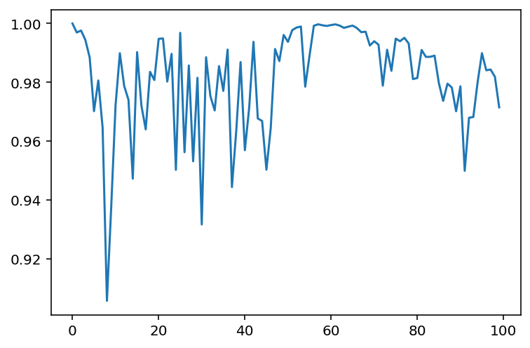
Q: Who was the first US president? A: George Washington ($0.999$) and Abraham Lincoln ($3.1\times 10^{-06}$).

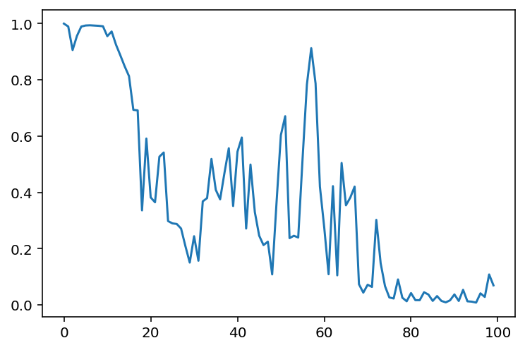
Q: Who is the author of The Grapes of Wrath? A: John Steinbeck ($\approx 1.0$) and Ernest Hemingway ($1.34\times 10^{-10}$).

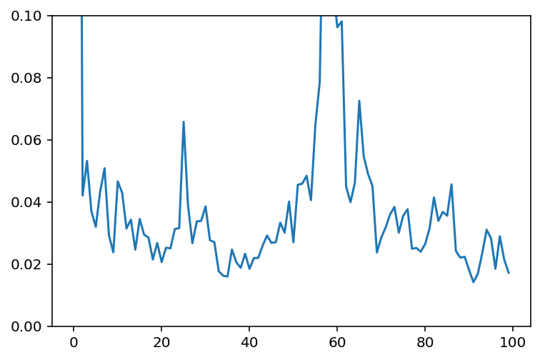
Q: What is the largest country in the world? A: Russia ($0.999$) and United Kingdom ($9.02\times 10^{-06}$).

Figure 1: Single-label queries with low epistemic uncertainty: Conditional normalized probability of the correct completion given repetitions of an incorrect response. Each figure shows the query and the considered two responses with their initial probabilities, as a response for the query, in parentheses (the first response is the correct one).

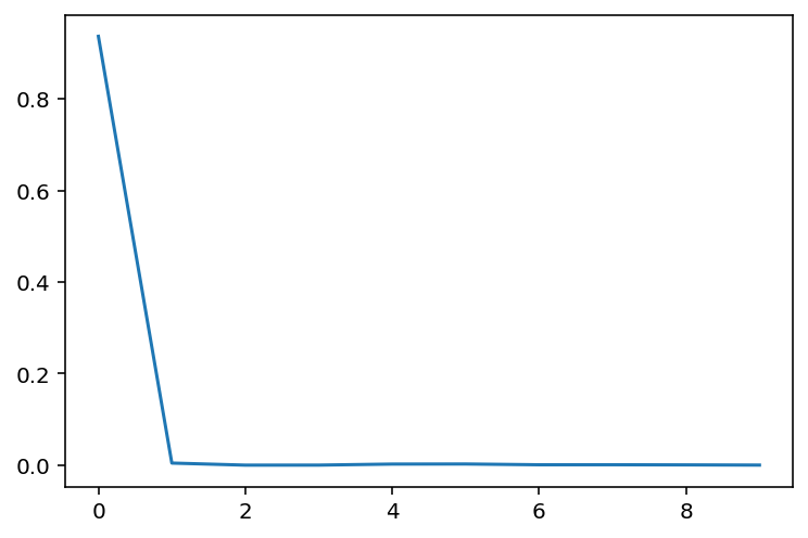
Q: What is the national instrument of Ireland? A: The harp ($0.936$) and Uilleann pipes ($0.063$).

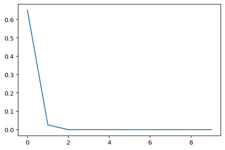
Q: Which actor became M in the Bond film Skyfall? A: Ralph Fiennes ($0.651$) and Judi Dench ($0.348$).

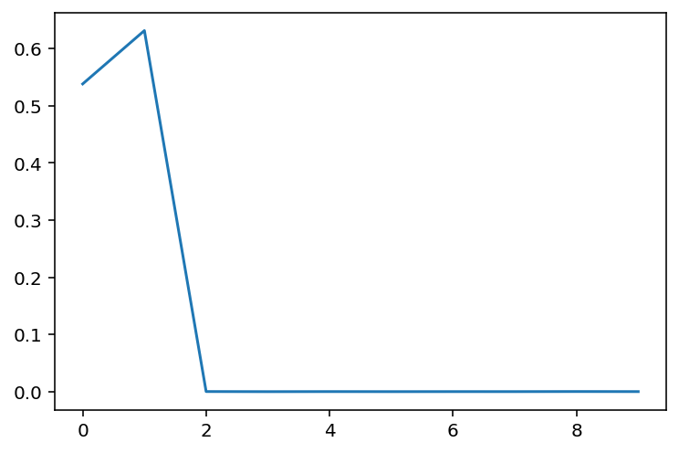
Q: Which can last longer with out water a camel or a rat? A: A rat ($0.538$) and A camel ($0.461$).

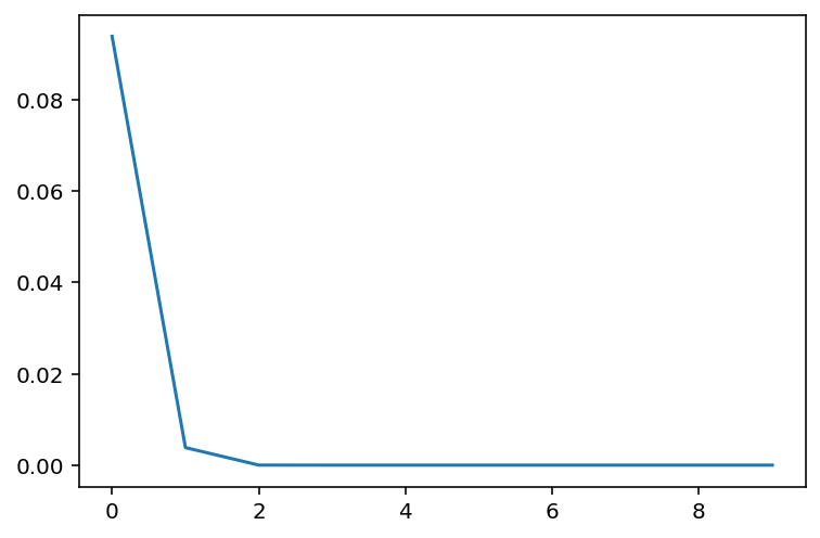
Q: If Monday’s child is fair of face what is Saturday’s child? A: Work hard for a living ($0.093$) and Full of grace ($0.906$).

Figure 2: Single-label queries with high epistemic uncertainty: Conditional normalized probability of the correct completion given repetitions of an incorrect response. Each figure shows the query and the considered two responses with their initial probabilities, as a response for the query, in parentheses (the first response is the correct one).

Next, we consider a queries for which the model is more uncertain. For the prompt “What is the national instrument of Ireland?”, we observe that responses “The harp” and “Uilleann pipes” both have significant probabilities (the first answer is the correct one). This time, by incorporating the incorrect response in the prompt multiple times, the probability of the correct answer quickly collapses to near zero, as shown in Figure 2, together with three more examples with significant epistemic uncertainty.

Finally, we consider multi-label queries for which the LLM confidently knows a correct answer. This time, by incorporating a potential response in the prompt, the probabilities of other correct answers stay relatively large. Figure 3 shows four such examples.

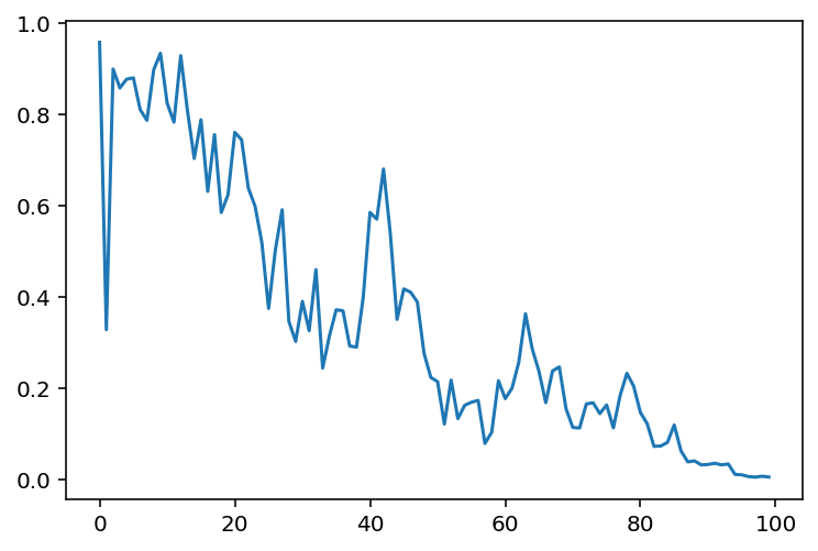
Q: Name a city in the UK A: London ($0.958$) and Manchester ($0.041$).

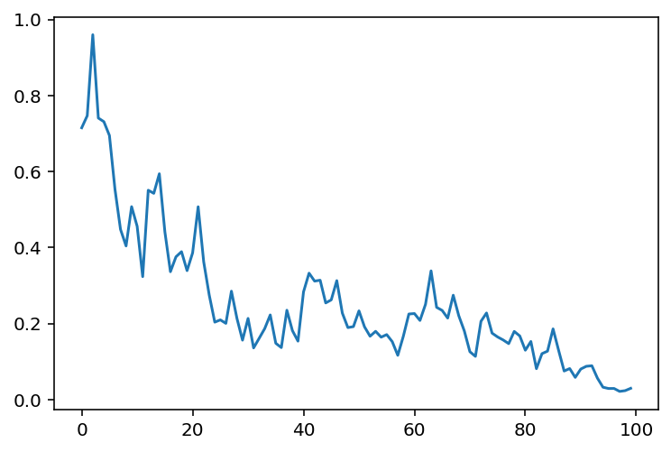
Q: Name a yellow fruit A: Banana ($0.715$) and Lemon ($0.284$).

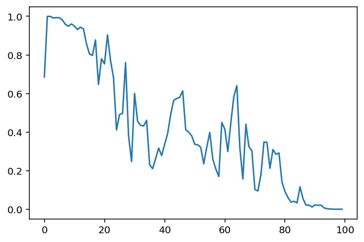
Q: Name an alcoholic drink, A: Wine ($0.685$) and Beer ($0.314$).

Q: Name a ball game that is played by more than 5 players A: Volleyball ($0.542$) and Soccer ($0.457$).

Figure 3: Multi-label queries with aleatoric uncertainty: Conditional normalized probability of the first of the two provided responses, both of which are correct, given repetitions of the second response in the prompt. Each figure shows the query and the considered two responses with their initial probabilities, as a response for the query, in parentheses.

3.1 In-context learning vs. in-weight learning

The sensitivity of the response of an LLM to extra in-context information, as observed above, can already be observed in a single attention head as explained next.

We consider an idealized attention mechanism as follows. Let ${\mathbf{Z}}\in{\mathbb{R}}^{n\times d^{\prime}}$ be an input matrix comprised of $n$ semantic feature vectors each of dimension $d^{\prime}$. Each row is meant to represent a complete statement (such as “What is the capital of the UK?” or “One answer to the question is Paris.”, etc.) rather than a single token. Let $X^{\top}\in{\mathbb{R}}^{1\times d^{\prime}}$ be the first row of ${\mathbf{Z}}$, which represents the query of interest, such as “What is the capital of the UK?”. Let $E^{\top}\in{\mathbb{R}}^{1\times d^{\prime}}$ be a special vector indicating the end of the input. The matrix ${\mathbf{Z}}\setminus X$, denoting the ${\mathbf{Z}}$ matrix without its first row, represents the in-context information.

We assume the ground-truth distribution $P$ is such that a query vector is mapped to its response, but a statement is simply copied. For example, for $V=\,$“What is the capital of the UK?”, $P(\,\cdot\,\mid V)$ would be a distribution with support on “London” and its variations, while for $V^{\prime}=\,$“What is the capital of the UK? One answer to the question is Paris.”, $P(\,\cdot\,\mid V^{\prime})$ returns the same distribution. We assume a parameter matrix ${\mathbf{W^{V}}}$ is learned such that $V^{\top}{\mathbf{W^{V}}}$ estimates $P(\,\cdot\,\mid V)$ for vector $V$.

Let ${\mathbf{W^{Q}}},{\mathbf{W^{K}}},{\mathbf{W^{V}}}\in{\mathbb{R}}^{d^{\prime}\times d}$ be the query, key, and value matrices. A self-attention head with query $X$ and context ${\mathbf{Z}}\setminus X$ is defined as

$$f({\mathbf{Z}};{\mathbf{W^{Q}}},{\mathbf{W^{K}}},{\mathbf{W^{V}}})=\text{Softmax}\left(\frac{1}{\sqrt{d}}E^{\top}{\mathbf{W^{Q}}}({\mathbf{Z}}{\mathbf{W^{K}}})^{\top}\right){\mathbf{Z}}{\mathbf{W^{V}}}\;$$

where the output of the Softmax is a row vector of length $n$.

If $X$ has appeared many times in the training data, then parameters ${\mathbf{W^{Q}}}$ and ${\mathbf{W^{K}}}$ could be learned such that $E^{\top}{\mathbf{W^{Q}}}({\mathbf{W^{K}}})^{\top}X$ is large, that is, $X$ is within the space spanned by the large principal components of the key-query matrix product. Then, no matter what in-context information appears in ${\mathbf{Z}}$, the probability assigned to $X$ will dominate the sotmax, and we will have

$$\text{Softmax}\left(\frac{1}{\sqrt{d}}E^{\top}{\mathbf{W^{Q}}}({\mathbf{Z}}{\mathbf{W^{K}}})^{\top}\right){\mathbf{Z}}\approx X^{\top}\,,$$

and therefore $f({\mathbf{Z}};{\mathbf{W^{Q}}},{\mathbf{W^{K}}},{\mathbf{W^{V}}})\approx P(\,\cdot\,\mid X)$.

On the other hand, consider the case that $X$ has not appeared many times in the training data, and vector $Y$ is copied in many rows of ${\mathbf{Z}}$. Then $E^{\top}{\mathbf{W^{Q}}}({\mathbf{W^{K}}})^{\top}X$ could be small as $X$ is not in the span of the large principal components of the key-query matrix product. Therefore $f({\mathbf{Z}};{\mathbf{W^{Q}}},{\mathbf{W^{K}}},{\mathbf{W^{V}}})\approx Y$ since

$$\text{Softmax}\left(\frac{1}{\sqrt{d}}E^{\top}{\mathbf{W^{Q}}}({\mathbf{Z}}{\mathbf{W^{K}}})^{\top}\right){\mathbf{Z}}\approx Y^{\top}\,.$$

Even if $X$ is in the span, repeating $Y$ $t$ times in ${\mathbf{Z}}$ would give a $t$-times increased total weight to $Y$ inside the softmax, which can dominate the weight assigned to $X$ when $t$ is large enough, also resulting in $Y$ as the answer.

4 Metric of epistemic uncertainty and its estimation

In this section we apply iterative prompting to estimate the epistemic uncertainty of a language model about responding to some query. The idea is to utilize the different behavior patterns observed in Section 3, which can be used to differentiate between two modes of high uncertainty: when the aleatoric uncertainty is high vs. when only the epistemic uncertainty is high. We then apply our new uncertainty metric to design a score-based hallucination detection algorithm.

Recall the family of prompts $\mathcal{F}$ defined in Section 2. We make the following assumption about the ground truth, which states that multiple responses to the same question drawn according to the ground truth are independent from each other:

Assumption 4.1 (Ground truth independence assumption).

The ground-truth satisfies

$$P(Y_{t}\mid F_{t-1}(x,Y_{1},\ldots,Y_{t-1}))=P(Y_{t}\mid x)\qquad\text{for any $t\in\mathbb{N}$ and any $x,Y_{1},\ldots,Y_{t}\in{\mathcal{X}}$.}$$

Note that the above assumption is heavily dependent on our prompt construction. Without embedding $Y_{1},\ldots,Y_{t-1}$ in the prompt, the independence assumption would not hold, for example, if $Y_{1},\ldots,Y_{t}$ were partial answers, such as a step of an algorithm or a part of a story, because in such a case $Y_{t}$ might indeed depend on the previous outputs $Y_{1},\ldots,Y_{t-1}$. Roughly speaking, the assumption tells that the response distribution is insensitive to a query based on previously sampled responses. For example, for query $x=$“A city in the UK:”, the probability of $Y_{2}=$“Manchester” does not change if a city is $Y_{1}=$“London”. Now we formally introduce a notion of the joint distribution over responses given a query, derived from the language model:

Definition 4.2 (Pseudo joint distribution).

Given a family of prompt functions $\mathcal{F}$, a conditional distribution $\mu\in{\mathcal{P}}$, and $n\in\mathbb{N}$, we use notation $\widetilde{\cdot}$ to denote a pseudo joint distribution defined as

$$\widetilde{\mu}(Y_{1},\dots,Y_{n}\mid x)=\mu(Y_{1}\mid F_{0}(x))\,\mu(Y_{2}\mid F_{1}(x,Y_{1}))\cdots\mu(Y_{n}\mid F_{n-1}(x,Y_{1},\ldots,Y_{n-1}))\;.$$ (1)

The above is a pseudo joint distribution since the standard conditioning in the chain-rule is replaced with prompt functions of the conditioning variables. In the following we focus on $\widetilde{Q}$ derived from the LLM and $\widetilde{P}$ derived from the ground truth.

Remark 4.3 (Sampling from $\widetilde{Q}$).

Note that sampling from $\widetilde{Q}$ can be simply done through a chain-rule-like procedure as can be seen from the above definition, that is, to have $(Y_{1},\dots,Y_{n})\sim\widetilde{Q}$ we draw $Y_{1}\sim Q(\cdot\mid F_{0}(x))$, $Y_{2}\sim Q(\cdot\mid F_{1}(x,Y_{1}))$, $Y_{3}\sim Q(\cdot\mid F_{2}(x,Y_{1},Y_{2}))$, and so on.

In the rest of the paper we drop subscripts in joint distributions and conditioning on query $x$ (which is understood implicitly), for example, $\widetilde{P}\equiv\widetilde{P}_{Y_{1}\cdots Y_{n}\mid x}$.

To measure epistemic uncertainty, we need to quantify how far the estimated pseudo joint distribution $\tilde{Q}$ is from the ground truth $\tilde{P}$. One natural choice is the following definition:

Definition 4.4 (Epistemic uncertainty metric).

Given an input $x\in{\mathcal{X}}$, we say that the epistemic uncertainty of $\widetilde{Q}$ is quantified by $D_{\mathrm{KL}}(\widetilde{Q},\widetilde{P})$.

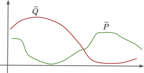
Figure 4: A hallucination: $\widetilde{Q}$ places an excessive mass where the ground truth $\widetilde{P}$ has a low mass.

Here $D_{\mathrm{KL}}$ measures how well $\widetilde{Q}$ approximates $\widetilde{P}$ for a given query $x$. Namely, this metric determines if $\widetilde{Q}$ assigns a large probability to an event which has a small probability under $\widetilde{P}$. In case of LLMs, this means the LLM generates a sequence that is unlikely in the typical usage of the language. In Figure 4 we have a situation where $\widetilde{P}$ is a pseudo joint distribution derived from the ground-truth, and $\widetilde{Q}$ suffers from a high hallucination rate. Given an input $x$, we want to estimate the above hallucination metric, but we only have access to $\widetilde{Q}$, and so computing it explicitly is impossible. However, next we show that under 4.1 we can lower bound $D_{\mathrm{KL}}(\widetilde{Q},\widetilde{P})$ by a quantity which only depends on $\widetilde{Q}$ (the proof is given in Appendix B).

Theorem 4.5.

For all pseudo joint distributions $\widetilde{P}$ satisfying 4.1, we have that

$$D_{\mathrm{KL}}(\widetilde{Q},\widetilde{P})\geq I(\widetilde{Q})~{}.$$

The lower bound in the theorem holds uniformly for all $\widetilde{P}$, and it is computable solely based on $\tilde{Q}$. This makes the bound applicable for decision making; in fact we chose to consider $D_{\mathrm{KL}}(\widetilde{Q},\widetilde{P})$ as the measure of epistemic uncertainty (out of many similar distance measures) because it admits this property).

Also, note that we have $I(\widetilde{Q})=D_{\mathrm{KL}}(\widetilde{Q},\widetilde{Q}^{\otimes})$ , $\widetilde{Q}^{\otimes}=\prod_{i}\sum_{y^{\backslash i}}\widetilde{Q}(y_{1},\ldots,y_{i-1},Y_{i},y_{i+1},\ldots,y_{n})$. In general $\sum_{y^{\backslash i}}\widetilde{Q}(y_{1},\ldots,y_{i-1},Y_{i},y_{i+1},\ldots,y_{n})\not=\widetilde{Q}(Y_{i})$, because the independence assumption 4.1 does not necessarily (and, in practice, almost never) holds for $Q$.

Finally, a quantity related to $D_{\mathrm{KL}}(\widetilde{Q},\widetilde{P})$ is $D_{\mathrm{KL}}$ with arguments arranged in the opposite order, that is $D_{\mathrm{KL}}(\widetilde{P},\widetilde{Q})$ which is a (query) conditional excess risk of the LLM-derived pseudo joint distribution $\widetilde{Q}$, under the logarithmic loss. Controlling the excess risk (for instance, upper-bounding it) for various algorithms is one of the central questions in learning theory, however it is a much harder task than the one we consider here, because for the former we need to theoretically control all sources of errors (such as generalization, estimation, and approximation error).

4.1 A computable lower bound on epistemic uncertainty

Theorem 4.5 gives a lower bound on the epistemic uncertainty by the mutual information. However, to compute the mutual information term, in practice we need to evaluate $\widetilde{Q}$ on its entire support, which is potentially infinite. Practically speaking, it is impossible to observe probabilities of all strings under the language model and so we must rely on a finite sample. Therefore, we replace $\widetilde{Q}$ with an empirical distribution with a finite support; in the following we show that the error induced by such an approximation is controlled. To estimate the MI we employ the method given in Algorithm 1; for generality it is presented for an arbitrary (pseudo) joint distribution $\mu$, but we keep in mind that our case of interest is $\mu=\widetilde{Q}$.

Algorithm 1 MI estimator

1:  Input: $\mu\in{\mathcal{M}}_{1}({\mathcal{X}}^{n})$ any (pseudo-) joint distribution over ${\mathcal{X}}^{n}$  $k\in\mathbb{N}$ sample size  $\gamma\geq 0$ stabilization parameter (typically selected as $1/k$)

2:  Independently sample tuples $X_{1},\,\ldots,\,X_{k}\sim\mu\in{\mathcal{M}}_{1}({\mathcal{X}}^{n})$

3:  Construct a set of indices of unique elements $S=\big{\{}i\in[k]~{}:~{}X_{i}\neq X_{j}\quad\forall j<i\big{\}}$

4:  Construct empirical distributions: for all $i\in S$,

$$\widehat{\mu}(X_{i}) =\frac{\mu(X_{i})}{Z}~{},$$

$$\widehat{\mu}^{\otimes}(x^{\prime}) =\prod_{i=1}^{n}\frac{\sum_{x^{\backslash i}}\mu(x_{1},\ldots,x_{i-1},x_{i}^{\prime},x_{i+1},\ldots,x_{n})}{Z^{\otimes}}\qquad\text{(for all $x^{\prime}\in{\mathcal{X}}^{n}$)}$$

where $$Z=\sum_{j\in S}\mu(X_{j})~{},\quad Z^{\otimes}=\sum_{j\in S}\sum_{x^{\backslash i}}\mu(x_{1},\ldots,x_{i-1},X_{j,i},x_{i+1},\ldots,x_{n})$$

5:  Compute estimate

$$\widehat{I}_{k}(\gamma)=\sum_{i\in S}\widehat{\mu}(X_{i})\,\ln\left(\frac{\widehat{\mu}(X_{i})+\gamma/Z}{\widehat{\mu}^{\otimes}(X_{i})+\gamma/Z^{\otimes}}\right)$$

Note that the estimator is constructed using only each unique element in the sample (the indices of these representative elements are collected in $S$), that is, we do not account for duplicate samples. Also note that most terms in the summations defining the product distribution $\widehat{\mu}^{\otimes}$ are zero (except the ones which correspond to the observed data). Furthermore, adding $\gamma/Z$ and $\gamma/Z^{\otimes}$ in the estimator $\widehat{I}_{k}(\gamma)$ is intended to account for the total probability of missing observations, not included while constructing $\widehat{\mu}$ and $\widehat{\mu}^{\otimes}$, making sure the estimate is bounded. Similar ideas are well-know in probability and information theory, such as in universal coding (cesa2006prediction), Laplace smoothing (Polyanskiy and Wu, 2024) and Good-Turing smoothing (Gale and Sampson, 1995, McAllester and Schapire, 2000).

The bias introduced by $\gamma$ in the last equation allows us to rigorously bound the error in estimating $I(\mu)$ via $\widehat{I}_{k}(\gamma)$, which is explored next. In particular, in Theorem 4.6 we prove a high-probability lower bound on $I(\mu)$ in terms of $\widehat{I}_{k}$. The core of controlling the estimation error is in accounting for the missing mass, or in other words, how much of $\mu$ we miss out by only observing a finite sample. In Appendix C, we present a more complete discussion and the proof of the bound on the estimation error for mutual information. Here we adapt this result to our particular case.

Define the missing mass as

$$U_{k}=\sum_{x\in{\mathcal{X}}^{n}}\mu(x)\,\mathbb{I}\big{\{}x\not\in\{X_{1},\ldots,X_{k}\}\big{\}}~{}.$$

Using this quantity, we are ready to present a non-asymptotic bound on the estimation error, which depends on the estimator $\widehat{I}_{k}(\gamma)$, the expected missing mass, and the sample size:

Theorem 4.6.

Suppose that $\widehat{I}_{k}(\gamma)$ is given by Algorithm 1, and assume that ${\mathcal{X}}$ is finite. For $\gamma=1/(k\,|{\mathcal{X}}^{n}|)$, with probability at least $1-\delta$,

$$I(\mu)\geq(1-\varepsilon_{k})\,\widehat{I}_{k}(\gamma)-\left(\frac{1}{k}+(1+n\,\ln\big{(}1+k\,|{\mathcal{X}}|)\big{)}\,\varepsilon_{k}\right)$$

$$\quad\text{where}\quad\varepsilon_{k}=\mathbb{E}[U_{k}]+\sqrt{\frac{\ln(\frac{1}{\delta})}{k}}~{}.$$

Furthermore, given $\delta_{\mathrm{supp}}\in[0,1)$, let $\tilde{\mathcal{X}}\subseteq{\mathcal{X}}^{n}$ such that $\mu(\tilde{\mathcal{X}})\geq 1-\delta_{\mathrm{supp}}$. Then, for $\gamma=1/(k\,|\tilde{\mathcal{X}}|)$, with probability at least $1-\delta$,

$$I(\mu)\geq(1-\varepsilon_{k})\,\widehat{I}_{k}(\gamma)-\left(\frac{1}{k}+(1+\ln\big{(}1+k\,|\tilde{\mathcal{X}}|)\big{)}\left(\delta_{\mathrm{supp}}+\varepsilon_{k}\right)\right)~{}.$$

The theorem is a corollary of Theorem C.4 shown in Appendix C. Note that in Theorem 4.6 we consider two bounds. The first one is pessimistic in the sense that it does not expect that the samples carry much information about the support, and it is most suitable in situations where we expect $\mu$ to be spread out (uniformly) across its entire support. The price of not having samples covering the whole support in this case is a factor $n\ln|{\mathcal{X}}|$ appearing in the bound. For example, in case of a language model with $10,000$ tokens, considering all possible strings of length $T$ tokens yields $n\ln|{\mathcal{X}}|=n\,T\ln(10000)$, and so

$$I(\mu)\geq(1-\varepsilon_{k})\,\widehat{I}_{k}(\gamma)-\left(\frac{1}{k}+(1+n\,T\ln\big{(}1+k\,\ln(10000))\big{)}\,\varepsilon_{k}\right)~{}.$$

Arguably, in practice, such situations are rare, as in natural languages we will not encounter all possible strings. To this end, we consider an optimistic scenario where the effective support of $\mu$, denoted by $\tilde{\mathcal{X}}$, is small with high probability. In this case, we can replace the size of the support for strings of length $n$, $|{\mathcal{X}}|^{n}$, in the first bound with the effective support size $|\tilde{\mathcal{X}}|$, and we only pay essentially a factor $\ln(1+k|\tilde{\mathcal{X}}|)$ instead of $n\ln(1+k|{\mathcal{X}}|)$. In case the effective sample size is only polynomial in $n$, this leads to an exponential reduction in $n$ for the second term in the bounds. In fact, in Section C.4 we demonstrate some empirical evidence that on two question-answering benchmarks, $|\tilde{\mathcal{X}}|$ rarely exceeds $\approx 100$ with $\mu(\tilde{\mathcal{X}})\geq 0.95$, while sampling responses from an LLM given a query.

Next we consider sufficient conditions for the estimator to converge to the mutual information. In particular, using the first bound in the theorem, we have (hiding logarithmic factors)

$$I(\mu)=\tilde{\Omega}\Big{(}(1-\mathbb{E}[U_{k}])\,\widehat{I}_{k}(\gamma)-\mathbb{E}[U_{k}]\Big{)}\qquad k\to\infty~{}.$$

This tells us that the rate of estimation error is essentially controlled by the expected missing mass $\mathbb{E}[U_{k}]$, which, as we will see, converges to zero as $k\to\infty$, however the decay can be very slow in general. For example, it is known that for a finite support of size $N$, $\mathbb{E}[U_{k}]\leq e^{-\frac{k}{N}}$ when $k\leq N$ and $\mathbb{E}[U_{k}]\leq N/(e\,k)$ otherwise (Berend and Kontorovich, 2012). For countable distributions with entropy bounded by $h$, one has $\mathbb{E}[U_{k}]\leq h/\ln(k)$ (Berend et al., 2017).

Despite these pessimistic bounds, in reality we expect the expected missing mass to be significantly smaller, especially when $\mu$ is heavy-tailed. It is well-known that natural languages (and many artificial ones) follow a Zipf distribution, where probability of each word (or a text piece) is proportional to $1/\mathrm{freq(text)}^{\alpha}$ for some exponent $\alpha>1$, where $\mathrm{freq}()$ is a frequency of occurrence in the corpus (Piantadosi, 2014). Then, we expect that $\mathbb{E}[U_{k}]$ should be much smaller than in such a case, since sampling from the tail of Zipf distribution is a rare event. To this end, in Appendix C we show that if $\widetilde{Q}$ is Zipf with exponent $\alpha>1$, then for any free parameter $\beta>0$,

$$\mathbb{E}[U_{k}]=\mathcal{O}\Big{(}k^{-(\frac{\alpha-1}{\alpha}-\beta)}\Big{)}~{}.$$

Hence, the rate at which the expected missing mass vanishes can be very fast (potentially matching a concentration rate $1/\sqrt{k}$ for $\alpha=2$).

Finally in Section C.4 we present a data-dependent estimation of $\mathbb{E}[U_{k}]$ based on a concentration inequality for a missing mass and repetitive sampling from LLM, in the context of some Q/A datasets. We conclude that the expected missing mass is very small: Most of the upper bounds on the expected missing mass (we have one upper bound per question) are highly concentrated close to $0$.

5 Score-based hallucination tests

Let $\widehat{I}_{k}(\gamma,x)\equiv\widehat{I}_{k}(\gamma)$ computed as in Algorithm 1 for $\mu=\widetilde{Q}$, to emphasize the explicit dependence on the query $x$. The uncertainty estimate $\widehat{I}_{k}(\gamma,x)$ derived above can be used as a score indicating the strength of our belief that the LLM hallucinates for the given query $x$. Such a score can then be used to design abstention policies: if the response is deemed to be hallucinated, the system abstains from responding, while a response is provided otherwise. Score-based abstention methods usually compute a score chosen by the user (such as the response likelihood or the estimator $\widehat{I}(\gamma)$ discussed earlier), and declare hallucination if the score is above or below a threshold, which is determined through calibration. To detect hallucinations successfully, the threshold can be adjusted through calibration on a given task using a hold-out (ground-truth) sample, see, for instance, the paper of Yadkori et al. (2024) where this calibration is discussed in detail.

Given our estimated lower bound on the epistemic uncertainty, we can define an abstention policy (a policy which decides when the LLM should abstain from prediction) as

$$a_{\lambda}(x)=\begin{cases}0,&\text{ if }\ \widehat{I}_{k}(\gamma,x)<\lambda;\\ 1,&\text{ if }\ \widehat{I}_{k}(\gamma,x)\geq\lambda;\end{cases}$$

where $\lambda>0$ is a threshold parameter tuned on a hold-out sample of some particular task. This policy abstains ($a_{\lambda}(x)=1$) when the epistemic uncertainty in the prediction (response) is large. When the policy does not abstain ($a_{\lambda}(x)=0$), any prediction from $\widehat{Q}$ can be served.

In the experiments, we compare a number of scoring functions for detecting hallucinations, including $\widehat{I}(\gamma)$, the probability of the greedy (temperature zero) response, and an estimate of the entropy of the response distribution.

6 Experiments

In this section we evaluate our abstention method derived based on the MI estimate in Section 5 on a variety of closed-book open-domain question-answering tasks.

Language model. We used a Gemini 1.0 Pro model (Gemini Team, Google, 2023) to generate outputs and scores.

Datasets. We consider three different datasets and their combinations: As base datasets, we consider (i) a random subset of $50,000$ datatpoints from the TriviaQA dataset (Joshi et al., 2017), and (ii) the entire AmbigQA dataset (with $12038$ datapoints) (Min et al., 2020). These datasets mostly contain single-label queries, and only contain a few multi-label ones. Moreover, we created a multi-label dataset based on the WordNet dataset (Fellbaum, 1998): We extracted all (6015) datapoints from WordNet at depth $4$ or more of the physical_entity subtree. For each datapoint (entity, children) in WordNet, we constructed a query of the form “Name a type of entity.” and children are considered target labels.

Comparison of responses and computing the output distributions. We use the F1 score thresholded at $0.25$ to decide if two text sequences match. When multiple responses are sampled, we approximate the output distribution of an LLM in a semantically meaningful way by collapsing matching responses into a single response: we sample $k=10$ responses at temperature $0.9$ for each query, and all those that match (according to the F1 score) are considered identical and their probabilities are aggregated. We only consider queries for which the greedy (temperature zero) and at least one of the random responses are shorter than $20$ characters. This is because the F1 score (as a match function) and log-probabilities (as a measure of uncertainty) are less reliable for longer sequences. After this filtering, we are left with $38870$ datapoints for TriviaQA, $5315$ datapoints for AmbigQA, and $3296$ datapoints for WordNet.

Baselines. We consider abstention policies based on four scoring methods. The first three are as follows: (i) the probability of the greedy response (denoted by $T0$); (ii) the semantic-entropy method of Kuhn et al. (2023) whose score is the entropy of $k=10$ generated samples (denoted by S.E.). To calculate entropy, we first aggregate probabilities of equivalent responses and normalize the probabilities so that they sum to 1 (as described above); and (iii) our proposed mutual information score as defined in Section 4 (and denoted by M.I.) with the choices of $k=10$, $n=2$, and $\gamma=0$ (the latter choice approximates the case that the number of potential responses can be very large in which case the theoretical choice of $\gamma$ would be very small). To calculate the mutual information, we first generate $k=10$ random samples. Then for any response $Y$, we calculate the probability of all generated responses given the prompt $F_{1}(x,Y)$. We construct estimates $\widehat{Q}(Y)$ and $\widehat{Q}(Y^{\prime}|Y)$ by aggregating probabilities of equivalent responses, and normalizing the probabilities so that they sum to 1.

Each baseline also has a default choice which is taken when the relevant score is above a threshold, and hence the method does not abstain. For $T0$, the default choice is the greedy (temperature zero) response. For S.E., the default choice is the response with the highest (aggregate) probability among the generated random responses. For the M.I. method, the default choice is the sampled response with the highest probability according to the marginalized pseudo joint distribution.

We also consider a version of the self-verification method of Kadavath et al. (2022) (denoted by S.V.) that, for a query $x$, first finds $Y_{1}$, the element with the largest (aggregated) probability (which is the default choice of S.E. method), and then calculates the probability of token “True” (normalized for the two tokens “True” and “False”) for the following query: “Consider the following question: Q: $x$. One answer to question Q is $Y_{1}$. Is the above answer to question Q correct? Answer True or False. A:”. The default choice of this baseline is the same as the default choice of the S.E. method. By this design, our intention is to construct a score that (unlike the first-order scores we consider) is not sensitive to the size of the label set.

In our experiments we either sweep through all abstention thresholds (Figure 5), or optimize the threshold on some calibration data, as explained in the description of the relevant experiment (Figure 6).

Results. We consider the precision-recall (PR) trade-off for the various methods on the different datasets. Here, recall is the percentage of queries where the method does not abstain, and precision is the percentage of correct decisions among these queries. Figure 5ab show PR-curves for the baselines and the proposed method on TriviaQA and AmbigQA. As can be seen, our method is better than the $T0$ and S.V. baselines, but performs similarly to the S.E. method. This is because the TriviaQA and AmbigQA datasets contain mostly single-label queries, and therefore a first-order method such as S.E. is sufficient to detect hallucinations. The AmbigQA dataset contains a few multi-label queries, but upon closer inspection, we observe that the LLM has low entropy on most of these queries. Therefore, a first-order method can perform as well as our method on such queries. Our proposed method, as well as the baselines, make no mistakes on the WordNet dataset (as the prediction of the LLM is always correct), hence we omit those results. The S.V. baseline performs significantly worse than the other methods when the recall is not high (is below about 0.8).

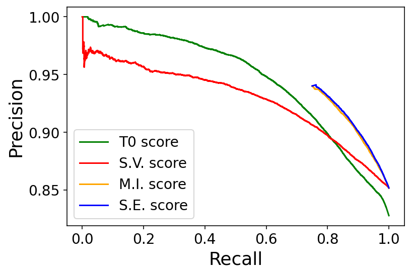
(a) TriviaQA

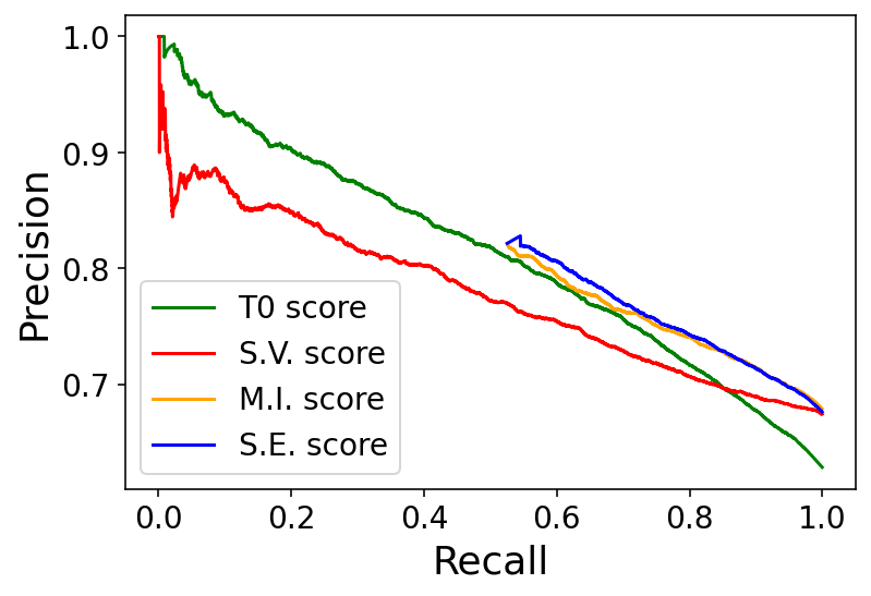
(b) AmbigQA

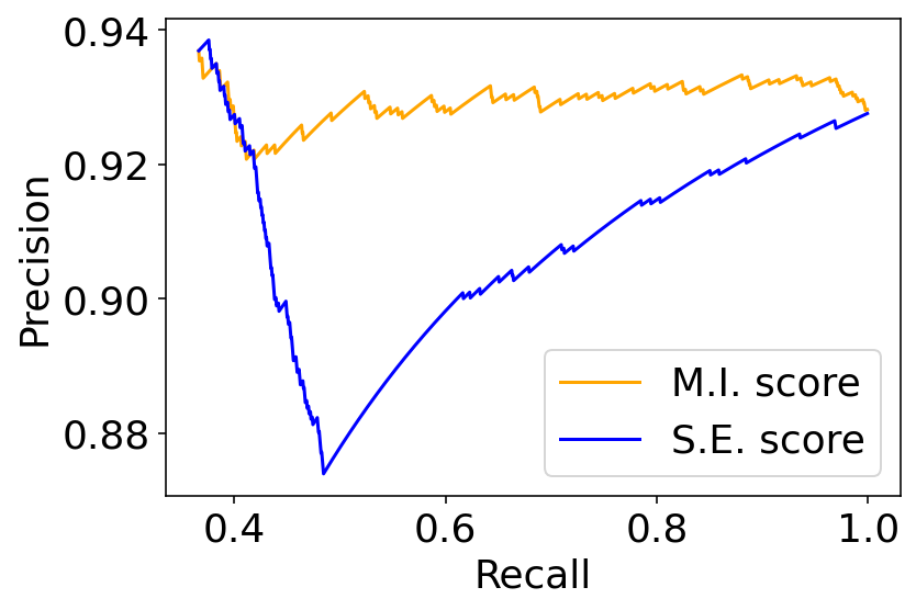
(c) TriviaQA+WordNet

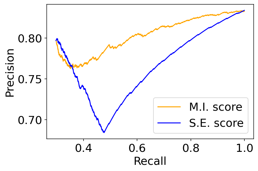
(d) AmbigQA+WordNet

Figure 5: PR-curve for the baseline and the proposed methods on various datasets. On the TriviaQA and AmbigQA datasets, M.I. and S.E. perform nearly identically, but they outperform the $T0$ and S.V. baselines. For the S.E. and M.I. methods, the responses for a large number of queries can be clustered into a single group, and therefore the semantic entropy and mutual information scores are zero. This is why the starting point of their curves is at a higher recall values. On the TriviaQA+WordNet and AmbigQA+WordNet datasets with a significant number of high entropy multi-label queries, M.I. outperforms the S.E. baseline. The methods perform nearly identical on the recall area that is not shown.

The similar performance for the S.E. and M.I. methods shown in Figure 5ab is due to the fact that the LLM has low entropy on most multi-label queries. However, ideally, an LLM should have higher entropy on multi-label queries (which would demonstrate broader knowledge, not focusing on a single possible answer). To include such queries, we mix the TriviaQA and AmbigQA datasets with our WordNet-based dataset with “truely” multi-label queries as constructed above. To enhance the intended effect, we filter our WordNet dataset by keeping only queries with entropy higher than $0.7$ (approximately the entropy of the uniform distribution over two atoms). Then we have $842$ remaining datapoints in WordNet. Note that when considered in isolation, both our proposed method and the semantic entropy method rarely make mistakes on this dataset. Then we create two new datasets by combining our $842$ WordNet datapoints with $842$ randomly selected datapoints from TriviaQA and AmbigQA, respectively, resulting in the TriviaQA+WordNet and AmbigQA+WordNet datasets. Figure 5cd show PR-curves for the S.E. and M.I. methods on these two combined datasets. Apart from low recall values, the performance of the S.E. method degrades noticeably with the addition of extra multi-label data. This precision/recall curve might look somewhat strange (with precision sometimes increasing with recall); this is due to the fact that both methods are always correct on the large number of high-entropy WordNet queries, where the LLM’s default predictions are correct.

The hardness with the combined datasets is that the predominantly single-label datasets (TriviaQA, AmbigQA) might need a different calibration threshold than the multi-label WordNet dataset, and this is better handled by our proposed method than by S.E. To better illustrate the improved abstention properties of our method, we examine how the two methods handle when the output of the LLM is diverse (i.e., has high entropy). In order to do this, we perform the following experiment: We create a calibration dataset by adding $500$ random datapoints from the WordNet dataset to $500$ random datapoints from TriviaQA, and another such random dataset for test. We determine the abstention thresholds on the calibration dataset for both the S.E. and the M.E. methods, and measure the performance (error rate, i.e., 1 minus precision, and recall) of the resulting abstention policies on the test set. We repeat this process $10$ times and report mean values and 95% confidence intervals with Gaussian approximation. We perform a similar evaluation process for mixtures of AmbigQA and WordNet datasets. Figure 6 show that while the S.E. method has similar recall and error rates to those of the proposed method on low-entropy queries, its recall values are much lower for queries with higher entropy, while the M.E. method makes only few mistakes on these queries.

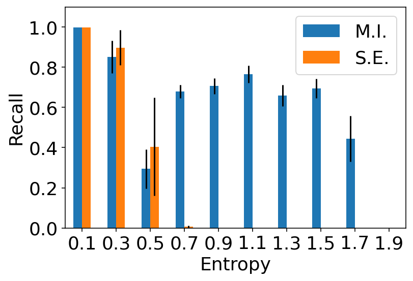
(a) TriviaQA+WordNet

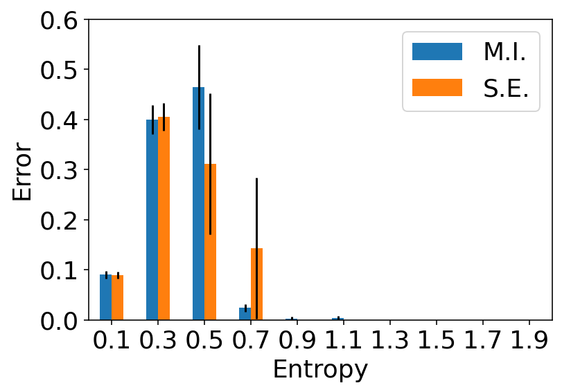
(b) TriviaQA+WordNet

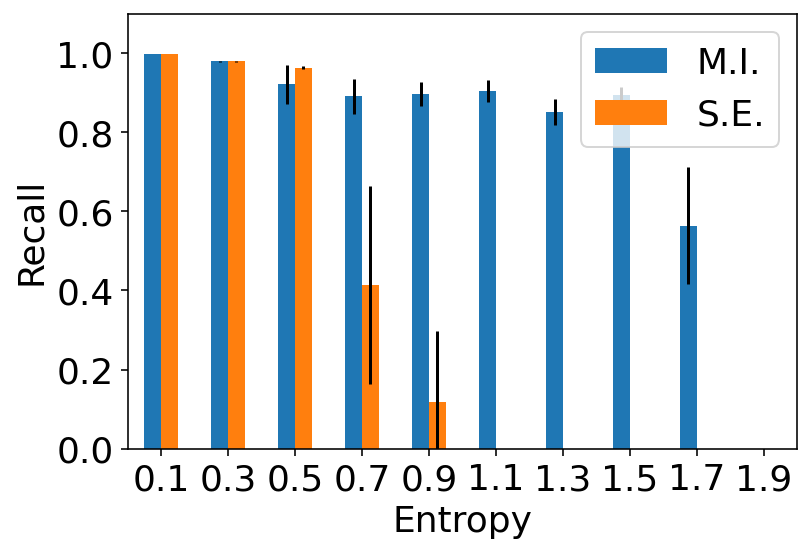
(c) AmbigQA+WordNet

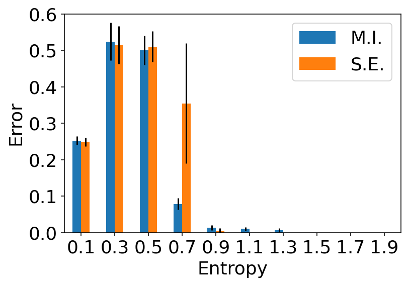
(d) AmbigQA+WordNet

Figure 6: Recall and error rates (one minus precision: percentage of mistakes when not abstaining) of the proposed and the baseline method on TriviaQA+WordNet and AmbigQA+WordNet datasets. On TriviaQA+WordNet and AmbigQA+WordNet datasets, the methods are calibrated at target loss of $0.05$ and $0.15$, respectively. On the x-axis, the queries are partitioned according to the entropy of the LLM’s output. Error bars show 2 standard deviation confidence intervals (based on 10 repetitions). While the first-order S.E. method has similar recall and error rates to those of the proposed M.E. method on low-entropy queries, its recall values are nearly zero for queries with higher entropy.

7 Conclusions

In this paper we considered epistemic uncertainty as a proxy for the truthfulness of LLMs. We proposed a mutual-information-based uncertainty estimator that admits a provable lower bound on the epistemic uncertainty of the LLM’s response to a query. That we consider joint distributions of multiple answers allows us to disentangle epistemic and aleatoric uncertainty, which makes it possible to better detect hallucination than first order methods, which can only tackle uncertainty as a whole, not epistemic uncertainty alone. This approach yielded an abstention method that performs significantly better on mixed single-label/multi-label datasets than first-order methods. While earlier methods for classification that aim to quantify epistemic uncertainty are usually based on a modified training method using response-tuples, utilizing the sequential nature of LLMs, our method does not need to change the training procedure, but needs to prompt the model iteratively with multiple responses generated by the LLM for the same query.

Appendix A Related works

In this section we present an overview of the related literature.

A.1 Training models with pairs of responses

Wen et al. (2022), Osband et al. (2023), Johnson et al. (2024) show that we can distinguish between epistemic and aleatoric uncertainty if we train the models with paired observations.

A.2 Epistemic neural nets

Ensemble methods are based on the classical idea of bootstrap for confidence estimation (Tibshirani and Efron, 1993), where multiple estimators for the regression function, each computed on a perturbed version of the data (e.g., by drawing samples from the empirical distribution over the data), are combined.

The empirical distribution of the resulting estimates is then used to construct confidence intervals. While many of these methods can be interpreted as sample-based approximations to Bayesian methods, model-hyperparameter selection (e.g., scale of perturbations, learning) for ensemble methods is typically done using a validation on holdout data (a subset of the training data). Many recent papers have studied ensemble methods in the context of deep learning and reinforcement learning (Osband et al., 2016, Lakshminarayanan et al., 2017a, Malinin and Gales, 2020). In the context of LLMs, the methods require training multiple language models, which is very expensive. Osband et al. (2023) introduces epistemic neural networks (epinets), which approximate ensemble methods by training a single network with an artificially injected (controlled) source of randomness. Rabanser et al. (2022) proposes to use intermediate model checkpoints to quantify the uncertainty of the final model in its responses. While these approaches aim to mimic the bootstrap procedure during prediction, their validity is not justified by theoretical considerations, and hence remain heuristic approximations.

A.3 Hallucination detection using first-order methods

First-order methods consider variance in the response distribution as a measure of hallucination (Kadavath et al., 2022, Cole et al., 2023, Manakul et al., 2023, Lin et al., 2023, Kuhn et al., 2023, Wang et al., 2022, Jiang et al., 2024, Zhang et al., 2023, Zhao et al., 2024, Yadkori et al., 2024). A common limitation of these approaches is that they are only applicable to prompts where there exists a single correct response, as they aim for detecting if one response (or multiple responses with the same meaning) is dominant. On the other hand, when multiple responses are correct, there is an aleatoric uncertainty in the ground truth: If an LLM correctly assigns non-negligible scores to multiple correct responses, most of these (if not all) will be declared as hallucination since, by design, only very few (typically at most one) responses can have scores higher than the threshold at the same time. Thus, hallucination detectors unaware of aleatoric uncertainty will invalidate most of the correct answers.

Yona et al. (2024) design a method that generates multiple responses, and then aggregates them into a single response at a (typically higher) granularity level where no further uncertainty (contradiction) is left compared to the generated responses. Although not a strictly first order method, it does not differentiate between aleatoric and epistemic uncertainty.

A.3.1 Asking language models to quantify uncertainty (self-verification)

Kadavath et al. (2022) propose to use LLM self-prompting to measure a model’s uncertainty in its responses. More specifically, for a given query, a number of responses are generated, and then the model is queried if the responses are correct. For this query, the log-probability of “True" is returned as a measure of uncertainty. Related approaches are studied by Mielke et al. (2022).

A.4 Uncertainty estimation based on sensitivity to contexts

Kassner and Schütze (2020) show that an LLM’s responses can be influenced by irrelevant contexts. Longpre et al. (2021), Neeman et al. (2022) study two sources of knowledge: parametric knowledge stored in the network weights, and contextual knowledge retrieved from external sources. They view reliance of the model on its parametric knowledge and ignoring relevant contextual information as hallucination. These works are mainly motivated by situations where the LLM’s knowledge is outdated and it is instructed to use the (new) contextual information. Accordingly, they design strategies to prioritize contextual information over parametric knowledge. Longpre et al. (2021) also show that larger models are more likely to ignore in-context information in favor of in-weight information. They propose creating training data with modified contextual information so that the model learns to favor the contextual information. Neeman et al. (2022) propose to train a model that predicts two answers: one based on parametric knowledge and one based on contextual information.

Similarly to Neeman et al. (2022), Li et al. (2023) aims to design a mechanism such that the model’s behavior is influenced more by relevant context than by its parametric knowledge (controllability), while the model is robust to irrelevant contexts (robustness). They improve controllability and robustness using finetuning.

Hou et al. (2024) study an approach to estimate model uncertainty due to ambiguity in a question. For a given question, their method generates multiple input clarification questions, and a new question is formed by augmenting the original question with each clarification question. The clarification questions are generated using an LLM with the aim of removing ambiguity in the question. This is different than the problem we study as the model can be uncertain about the answer even if the query itself has no ambiguity. For such queries, the method of Hou et al. (2024) might decide that no clarification is needed, and therefore there is no uncertainty.

A.5 Hallucination detection using internal states of LLMs

There are a number of papers that try to extract knowledge/truthfulness by inspecting hidden-layer activations of LLMs (Burns et al., 2023, Azaria and Mitchell, 2023, Chen et al., 2024). Such methods clearly require access to the LLM’s internal states, which is not always possible, and severely limits the applicability of these methods.

Appendix B Omitted proofs

Proof of Theorem 4.5.

In the following we will use abbreviations

$$\sum_{y}=\sum_{y_{1},\ldots,y_{n}}~{},\qquad\sum_{y^{\backslash i}}=\sum_{y_{1},\ldots,y_{i-1},y_{i+1},\ldots,y_{n}}$$

where each coordinate belongs to ${\mathcal{X}}$. Now,

$$D_{\mathrm{KL}}(\widetilde{Q},\widetilde{P}) =-H(\widetilde{Q})+\sum_{y}\widetilde{Q}(y_{1},\ldots,y_{n})\,\ln\frac{1}{\widetilde{P}(y_{1},\ldots,y_{n})}$$

$$=-H(\widetilde{Q})+\sum_{y}\widetilde{Q}(y_{1},\ldots,y_{n})\,\ln\frac{1}{\prod_{i}P\big{(}y_{i}\mid F_{i-1}(y_{1},\ldots,y_{i-1})\big{)}}$$ (using Definition 4.2)

$$=-H(\widetilde{Q})+\sum_{y}\widetilde{Q}(y_{1},\ldots,y_{n})\,\ln\frac{1}{\prod_{i}P(y_{i})}~{}.$$ (by the independence assumption)

Focusing on the last (cross-entropy) term

$$\sum_{y}\widetilde{Q}(y_{1},\ldots,y_{n})\,\ln\frac{1}{\prod_{i}P(y_{i})}$$

$$\quad=\sum_{y}\widetilde{Q}(y_{1},\ldots,y_{n})\,\sum_{i}\ln\frac{1}{P(y_{i})}$$

$$\quad=\sum_{i}\sum_{y_{i}}\sum_{y^{\backslash i}}\widetilde{Q}(y_{1},\ldots,y_{n})\,\ln\frac{1}{P(y_{i})}$$

$$\quad\stackrel{{\scriptstyle(a)}}{{\geq}}\sum_{i}\sum_{y_{i}}\sum_{y^{\backslash i}}\widetilde{Q}(y_{1},\ldots,y_{n})\,\ln\frac{1}{\sum_{y^{\backslash i}}\widetilde{Q}(y_{1},\ldots,y_{n})}$$

$$\quad=\sum_{y}\widetilde{Q}(y_{1},\ldots,y_{n})\,\ln\frac{1}{\prod_{i}\sum_{y^{\backslash i}}\widetilde{Q}(y_{1},\ldots,y_{n})}$$

where in $(a)$ we used the fact that entropy is no larger than cross-entropy. Thus,

$$D_{\mathrm{KL}}(\widetilde{Q},\widetilde{P})\geq\sum_{y}\widetilde{Q}(y_{1},\ldots,y_{n})\ln\frac{\widetilde{Q}(y_{1},\ldots,y_{n})}{\prod_{i}\sum_{y^{\backslash i}}\widetilde{Q}(y_{1},\ldots,y_{n})}=I(\widetilde{Q};Y_{1},\ldots,Y_{n})~{}.$$

∎

Appendix C Estimation of mutual information and missing mass problem

In this section, we discuss how to estimate the mutual information from a finite sample, which may not cover the full distribution. To control the estimation error, we first introduce the concept of missing mass.

C.1 The missing mass problem

Let ${\mathcal{X}}$ be a countable set and suppose that $X_{1},\ldots,X_{k}\sim\mu\in{\mathcal{M}}_{1}({\mathcal{X}}^{n})$ independently. In the following $x$ is used as an element of ${\mathcal{X}}^{n}$ rather than the query (as in Section 4). Then, the missing mass is defined as the random variable

$$U_{k}=\sum_{x\in{\mathcal{X}}^{n}}\mu(x)\,\xi(x)~{},\qquad\xi(x)=\mathbb{I}\{x\not\in\{X_{1},\ldots,X_{k}\}\}~{}.$$

Here we are primarily interested in two questions: (i) how quickly $U_{k}$ approaches the expected missing mass $\mathbb{E}U_{k}$, where it is not hard to see that

$$\mathbb{E}U_{k}=\sum_{x\in{\mathcal{X}}^{n}}\mu(x)(1-\mu(x))^{k}~{};$$

and (ii) we are also interested in giving an estimate for $\mathbb{E}U_{k}$ given $\mu$ and $k$. The first question is answered by the following theorem:

Theorem C.1 (Concentration of a missing mass (Berend and Kontorovich, 2013)).

For any $t>0$, we have an upper-tail bound

$$\mathbb{P}\left(U_{k}>\mathbb{E}U_{k}+t\right)\leq e^{-tk^{2}}~{},$$

and moreover for a universal constant $c\approx 7.6821$, we have an lower-tail bound

$$\mathbb{P}\left(U_{k}<\mathbb{E}U_{k}-t\right)\leq e^{-ctk^{2}}~{}.$$

Notably $U_{k}$ exhibits a sub-gaussian concentration (i.e. $1/\sqrt{k}$), which is surprisingly fast. As we will see next, the main bulk of the error incurred for missing a subset of the support is hidden in $\mathbb{E}U_{k}$.

In particular, when ${\mathcal{X}}$ is finite with $|{\mathcal{X}}|=N$, Berend and Kontorovich (2012) showed that

$$\mathbb{E}U_{k}\leq\begin{cases}e^{-\frac{n}{N}},&\text{ if }n\leq N;\\ \frac{N}{e\,n},&\text{ if }n>N.\end{cases}$$

In the countably infinite ${\mathcal{X}}$, we cannot generally have a non-trivial bound on $\mathbb{E}U_{k}$ only in terms of $n$. In fact, Berend and Kontorovich (2012) show a bound that depends on $\mu$ which is expected to be finite for rapidly decaying atoms. Interestingly, when the entropy of $\mu$ is bounded, one has the following result (Berend et al., 2017):

Theorem C.2.

Let $H(\mu)\leq h<\infty$. For all $n\geq 1$, we have $\mathbb{E}U_{k}\leq\frac{h}{\sum_{i=1}^{k}i^{-1}}\leq\frac{h}{\ln(n)}.$

Note that these estimates are very pessimistic, and in reality we expect the expected missing mass to be significantly smaller. Since natural (and many artificial) languages follow a Zipf distribution (Piantadosi, 2014), we expect that $\mathbb{E}[U_{k}]$ should be much smaller than in the above cases, since sampling from the tail of a Zipf distribution is a rare event. In Section C.4 we show the following:

Corollary C.3 (Expected missing mass of Zipf distribution).

Consider distribution $\mu(i)=i^{-\alpha}/H(\alpha,N)$ for $i\in[N]$, where $\alpha>1$ and $H(\alpha,N)=\sum_{i=1}^{N}i^{-\alpha}$. Then, for any $\beta>0$,

$$\mathbb{E}[U_{k}]=\mathcal{O}\Big{(}k^{-(\frac{\alpha-1}{\alpha}-\beta)}\Big{)}~{}.$$

Proof.

The statement followss by combining Lemmas C.7 and C.8. ∎

C.2 Estimating mutual information from the partial support

Our goal is to estimate

$$I(\mu)=D_{\mathrm{KL}}(\mu,\mu^{\otimes})=\sum_{x\in{\mathcal{X}}^{n}}\mu(x)\ln\left(\frac{\mu(x)}{\mu^{\otimes}(x)}\right)$$

by only having access to $X_{1},\ldots,X_{k}\sim\mu$. Note that that the sample might cover only some part of the support of ${\mathcal{X}}$ and therefore we are facing a missing mass problem. In the following we consider estimator $\widehat{I}_{k}(\gamma)$ given by Algorithm 1.

In particular in Section C.3 we show the following

Theorem C.4.

Fix $\tilde{\mathcal{X}}\subseteq{\mathcal{X}}^{n}$. For any fixed $\gamma>0,\delta\in(0,1)$, with probability at least $1-\delta$,

$$(1-\varepsilon_{k})\,\widehat{I}_{k}(\gamma)-\left(|\tilde{\mathcal{X}}|\gamma+\ln\left(e+\frac{e}{\gamma}\right)\left(\mu({\mathcal{X}}^{n}\setminus\tilde{{\mathcal{X}}})+\varepsilon_{k}\right)\right)\leq I(\mu)$$

where

$$\varepsilon_{k}=\mathbb{E}U_{k}+\sqrt{\frac{\ln(\frac{1}{\delta})}{k}}~{}.$$

In particular, Theorem C.4 implies the following:

Corollary C.5.

Under conditions of Theorem C.4, there exists $\gamma^{*}_{k}\in(0,1)$ such that

$$(1-\varepsilon_{k})\,\widehat{I}_{k}(\gamma^{*}_{k})-\left(\frac{1}{k}+(1+n\,\ln\big{(}1+k\,|{\mathcal{X}}|)\big{)}\,\varepsilon_{k}\right)\leq I(\mu)~{}.$$

Note that, choosing any of the upper bounds on $\mathbb{E}U_{k}$ discussed in Section C.1, we can see that Corollary C.5 implies asymptotic convergence in as a sense

$$\lim_{k\to\infty}\widehat{I}_{k}(\gamma^{*}_{k})\leq I(\mu)~{}.$$

C.3 Proof of Theorem C.4

The proof will heavily rely on the simple fact that

$$1-\xi(x)\,=\begin{cases}1,&\text{ if $x\in\{X_{1},\ldots,X_{k}\}$;}\\ 0,&\text{ otherwise.}\end{cases}$$ (2)

Recalling that $S=\big{\{}i\in[k]~{}:~{}X_{i}\neq X_{j}\quad\forall j<i\big{\}}$, this immediately implies the following connection between $U_{k}$ and the quantities used in Algorithm 1:

Proposition C.6.

We have that

$$\sum_{j\in S}\mu(X_{j})=\sum_{x\in{\mathcal{X}}^{n}}(1-\xi(x))\,\mu(x)=1-U_{k}~{}.$$

Recall that the product distribution of $\mu$ is defined as

$$\mu^{\otimes}(x)=\prod_{i=1}^{n}\sum_{x^{\backslash i}}\mu(x_{1},\ldots,x_{i-1},x_{i},x_{i+1},\ldots,x_{n})~{}.$$

Note that we use $\sum_{x^{\backslash i}}\mu(\cdots)$ instead of $\mu(x_{i})$ since these are not necessarily equal for some $\mu$.

Introducing a one-dimensional version of $\xi$, for $i\in[n]$ and $z\in{\mathcal{X}}$, as

$$\xi_{i}(z)=\mathbb{I}\{z\not\in\{X_{1,i},\ldots,X_{k,i}\}\}~{},$$

we introduce the normalization factors

$$Z=\sum_{x\in{\mathcal{X}}^{n}}(1-\xi(x))\mu(x)~{},\qquad Z^{\otimes}=\prod_{i=1}^{n}\sum_{z\in{\mathcal{X}}}(1-\xi_{i}(z))\sum_{x^{\backslash i}}\mu(x_{1},\ldots,x_{i-1},z,x_{i+1},\ldots,x_{n})~{}.$$

We first note that by the definition of $\widehat{\mu}^{\otimes}$, for any $x^{\prime}\in{\mathcal{X}}^{n}$,

$$\widehat{\mu}^{\otimes}(x^{\prime}) =\prod_{i=1}^{n}\frac{\sum_{x^{\backslash i}}\mu(x_{1},\ldots,x_{i-1},x_{i}^{\prime},x_{i+1},\ldots,x_{n})}{\sum_{j\in S}\sum_{x^{\backslash i}}\mu(x_{1},\ldots,x_{i-1},X_{j,i},x_{i+1},\ldots,x_{n})}$$

$$=\prod_{i=1}^{n}\frac{\sum_{x^{\backslash i}}\mu(x_{1},\ldots,x_{i-1},x_{i}^{\prime},x_{i+1},\ldots,x_{n})}{\sum_{z\in{\mathcal{X}}}(1-\xi_{i}(z))\sum_{x^{\backslash i}}\mu(x_{1},\ldots,x_{i-1},z,x_{i+1},\ldots,x_{n})}$$

$$=\frac{\mu^{\otimes}(x^{\prime})}{Z^{\otimes}}~{},$$

where the second equality comes from the definition of $\xi_{i}$ and the fact that the $X_{i}$ are all different. Now, using the definitions of $\widehat{I}_{k}$ and $\widehat{\mu}$,

$$\widehat{I}_{k}(\gamma) =\frac{1}{\sum_{j\in S}\mu(X_{j})}\sum_{i\in S}\mu(X_{i})\left(\ln\left(\frac{\mu(X_{i})}{\sum_{j\in S}\mu(X_{j})}+\frac{\gamma}{\sum_{j\in S}\mu(X_{j})}\right)-\ln\left(\widehat{\mu}^{\otimes}(X_{i})+\frac{\gamma}{Z^{\otimes}}\right)\right)$$

$$=\frac{1}{Z}\sum_{i\in S}\mu(X_{i})\left(\ln\left(\frac{\mu(X_{i})+\gamma}{Z}\right)-\ln\left(\frac{\mu^{\otimes}(X_{i})+\gamma}{Z^{\otimes}}\right)\right)$$ (by Proposition C.6)

$$=\frac{1}{Z}\sum_{x\in{\mathcal{X}}^{n}}(1-\xi(x))\,\mu(x)\left(\ln\left(\frac{\mu(x)+\gamma}{Z}\right)-\ln\left(\frac{\mu^{\otimes}(x)+\gamma}{Z^{\otimes}}\right)\right)$$ (by Eq. 2 )

$$\leq\frac{1}{Z}\sum_{x\in{\mathcal{X}}^{n}}(1-\xi(x))\,\mu(x)\left(\ln\left(\frac{\mu(x)+\gamma}{\mu^{\otimes}(x)+\gamma}\right)\right)+\ln\frac{Z^{\otimes}}{Z}$$

$$=\underbrace{\frac{1}{Z}\sum_{x\in{\mathcal{X}}^{n}}\mu(x)\ln\left(\frac{\mu(x)+\gamma}{\mu^{\otimes}(x)+\gamma}\right)}_{(i)}+\underbrace{\frac{1}{Z}\sum_{x\in{\mathcal{X}}^{n}}\xi(x)\,\mu(x)\ln\left(\frac{\mu^{\otimes}(x)+\gamma}{\mu(x)+\gamma}\right)}_{(ii)}+\underbrace{\ln\frac{{Z}^{\otimes}}{Z}}_{(iii)}~{}.$$

To control $(i)$ we will first need the fact that $q\ln((q+\gamma)/p)\leq q\ln(q/p)+\gamma$ for any $q,p\in[0,1],\gamma>0$. Note that this follows since

$$q\ln\left(\frac{q+\gamma}{p}\right)=q\ln\left(1+\frac{\gamma}{q}\right)+q\ln\left(\frac{q}{p}\right)\leq\gamma+q\ln\left(\frac{q}{p}\right)$$ (3)

using that $\ln(1+a)\leq a$ for $a>-1$. Getting back to $(i)$, and using the aforementioned inequality, we get

$$(i) =\frac{1}{Z}\sum_{x\in{\mathcal{X}}^{n}}\mu(x)\ln\left(\frac{\mu(x)+\gamma}{\mu^{\otimes}(x)+\gamma}\right)$$

$$=\frac{1}{Z}\sum_{x\in\tilde{{\mathcal{X}}}}\mu(x)\ln\left(\frac{\mu(x)+\gamma}{\mu^{\otimes}(x)+\gamma}\right)+\frac{1}{Z}\sum_{x\in{\mathcal{X}}^{n}\setminus\tilde{{\mathcal{X}}}}\mu(x)\ln\left(\frac{\mu(x)+\gamma}{\mu^{\otimes}(x)+\gamma}\right)$$

$$\leq\frac{1}{Z}\sum_{x\in\tilde{{\mathcal{X}}}}\mu(x)\ln\left(\frac{\mu(x)+\gamma}{\mu^{\otimes}(x)+\gamma}\right)+\frac{1}{Z}\,\ln\left(\frac{1+\gamma}{\gamma}\right)\,\mu({\mathcal{X}}^{n}\setminus\tilde{{\mathcal{X}}})$$

$$\leq\frac{1}{Z}\sum_{x\in\tilde{\mathcal{X}}}\left(\mu(x)\ln\left(\frac{\mu(x)}{\mu^{\otimes}(x)}\right)+\gamma\right)+\frac{1}{Z}\,\ln\left(1+\frac{1}{\gamma}\right)\,\mu({\mathcal{X}}^{n}\setminus\tilde{{\mathcal{X}}})$$ (by Equation 3)

$$=\frac{1}{Z}\left(D_{\mathrm{KL}}(\mu,\mu^{\otimes})+|\tilde{\mathcal{X}}|\,\gamma\right)+\frac{1}{Z}\,\ln\left(1+\frac{1}{\gamma}\right)\,\mu({\mathcal{X}}^{n}\setminus\tilde{{\mathcal{X}}})~{}.$$

Furthermore,

$$(ii)\leq\frac{1}{Z}\,\sum_{x\in{\mathcal{X}}^{n}}\xi(x)\,\mu(x)\ln\left(1+\frac{1}{\gamma}\right)=\frac{1-Z}{Z}\,\ln\left(1+\frac{1}{\gamma}\right)~{}.$$

Next, observe that $(iii)\leq\ln(1/Z)$. Finally, putting all together,

$$\widehat{I}_{k}(\gamma) \leq\frac{1}{Z}\left(D_{\mathrm{KL}}(\mu,\mu^{\otimes})+|\tilde{\mathcal{X}}|\gamma\right)+\frac{1}{Z}\,\ln\left(1+\frac{1}{\gamma}\right)\left(\mu({\mathcal{X}}^{n}\setminus\tilde{{\mathcal{X}}})+1-Z\right)+\ln(1/Z)~{}.$$

Finally, multiplying through by $Z$ the entire inequality, and using the fact that $Z\ln(1/Z)\leq 1-Z$, we get

$$Z\,\widehat{I}_{k}(\gamma) \leq D_{\mathrm{KL}}(\mu,\mu^{\otimes})+|\tilde{\mathcal{X}}|\gamma+\ln\left(1+\frac{1}{\gamma}\right)\left(\mu({\mathcal{X}}^{n}\setminus\tilde{{\mathcal{X}}})+1-Z\right)+1-Z$$

$$\leq D_{\mathrm{KL}}(\mu,\mu^{\otimes})+|\tilde{\mathcal{X}}|\gamma+\ln\left(e+\frac{e}{\gamma}\right)\left(\mu({\mathcal{X}}^{n}\setminus\tilde{{\mathcal{X}}})+1-Z\right)$$

To complete the proof we need to give a lower bound on $Z$. Note that $Z=1-U_{k}$ by the definition of $Z$ and Proposition C.6, and so by Theorem C.1

$$\mathbb{P}\left(1-\mathbb{E}U_{k}>1-U_{k}+t\right)\leq e^{-tk^{2}}~{}.$$

Using this concentration bound together with the choices of $\gamma$ (also setting $\delta_{\mathrm{supp}}=0$ for the first inequality in the main statement) completes the proof of Theorem C.4. $\square$

C.4 Expected missing mass under Zipf distribution

We will rely on some machinery used by Ohannessian and Dahleh (2010) who established distribution-dependent bounds on the expected missing mass. As before let $\mu$ be supported on a countable set. The accrual function is defined as

$$F(v)=\sum_{\mu(i)\leq v}\mu(i)\qquad(v\in[0,1])$$

and moreover the accrual rates are defined as

$$\underline{\rho}=\liminf_{v\to 0}\frac{\ln F(v)}{\ln v}~{},\qquad\overline{\rho}=\limsup_{v\to 0}\frac{\ln F(v)}{\ln v}$$

We use the following result:

Lemma C.7 (Ohannessian and Dahleh, 2010, Theorem 1).

Let $\mu$ have lower and upper accrual rates $0<\underline{\rho}\leq\overline{\rho}<\infty$. Then for every $\beta>0$ there exists $k_{0}$ such that for all $k>k_{0}$ we have:

$$k^{-(\overline{p}+\beta)}\leq\mathbb{E}[U_{k}]\leq k^{-(\underline{p}-\beta)}$$

or, equivalently, for every $\beta>0$ we have that $\mathbb{E}[U_{k}]$ is both $\Omega(k^{-(\overline{p}+\beta)})$ and $\mathcal{O}(k^{-(\underline{p}-\beta)})$.

Proposition C.8.

Consider the distribution $\mu(v)=i^{-\alpha}/H(\alpha,N)$ for $i\in[N]$ where $\alpha>1$ and $H(\alpha,N)=\sum_{i=1}^{N}i^{-\alpha}$. Then, $\underline{\rho}=\Omega(\frac{\alpha-1}{\alpha})$ as $N\to\infty$.

Proof.

The idea is to use Lemma C.7 to give an upper bound on the missing mass. Therefore, we need to establish a lower bound on $\ln F(v)$. For now, abbreviate

$$u=(v\,H(\alpha,N))^{-\frac{1}{\alpha}}~{}.$$

First note that for some $1\leq u\leq N$

$$\sum_{i\geq u}^{N}i^{-\alpha}\geq\int_{u}^{N}(1+i)^{-\alpha}\mathop{}\!\mathrm{d}i=\frac{1}{\alpha-1}\,\left((1+u)^{1-\alpha}-(1+N)^{1-\alpha}\right)~{}.$$

On the other hand,

$$\sum_{i=1}^{N}i^{-\alpha}\leq\int_{1}^{N}(1+i)^{-\alpha}\mathop{}\!\mathrm{d}i\leq\frac{1}{\alpha-1}\,(1-N^{1-\alpha})~{}.$$

So,

$$\ln F(v) \geq\ln\left((1+u)^{1-\alpha}-(1+N)^{1-\alpha}\right)-\ln(1-N^{1-\alpha})$$

$$\geq\ln\left((1+u)^{1-\alpha}-(1+N)^{1-\alpha}\right)$$

and then

$$\ln F(v) =\Omega\left((1-\alpha)\ln(1+u)\right)\qquad(\text{as}\,N\to\infty)$$

$$=\Omega\left((1-\alpha)\ln(u)\right)$$

$$=\Omega\left((1-\alpha)\ln((v\,H(\alpha,N))^{-\frac{1}{\alpha}})\right)$$

$$=\Omega\left(\frac{\alpha-1}{\alpha}\,\ln(v)+\frac{\alpha-1}{\alpha}\ln H(\alpha,N)\right)$$

$$=\Omega\left(\frac{\alpha-1}{\alpha}\,\ln(v)\right)~{}.$$

∎

Data-dependent estimate of the expected missing mass

We perform an experiment designed to give a data-dependent estimate of the expected missing mass $\mathbb{E}[U_{k}]$ for some specific datasets. Clearly, we cannot simply apply a concentration bound discussed in Section C.1 since the complete support of the pseudo joint distribution derived from the LLM is unknown. To this end, we approximate it with a finite support driven by the language model itself. In particular, given a query we sample responses (at temperature $0.9$) until their total probability mass reaches $0.95$ or we reach $1000$ responses per query. In case of TriviaQA, we performed $1233$ queries in total. The mean and the median number of unique responses per query was eventually $118.3$ and $22$, respectively. In case of the AmbigQA dataset, we performed $700$ queries, while the mean and the median number of unique responses was $277$ and $69$, respectively.

At this point, we denote the set of responses by $\tilde{\mathcal{X}}$ and let $\tilde{U}_{k}$ be the missing mass computed on $\tilde{\mathcal{X}}$. Then, we have

$$\mathbb{E}[U_{k}]\leq U_{k}+\sqrt{\frac{\ln(\frac{1}{\delta})}{k}}\leq\tilde{U}_{k}+U_{k}-\tilde{U}_{k}+\sqrt{\frac{\ln(\frac{1}{\delta})}{k}}\leq\tilde{U}_{k}+1-P(\tilde{\mathcal{X}})+\sqrt{\frac{\ln(\frac{1}{\delta})}{k}}~{},$$

which can be computed in practice. In Figure 7 we present our results in the form of empirical distributions of different quantities, where each observation corresponds to a single query. We compute the bounds for TriviaQA and AmbigQA datasets (see Section 6 for details about these datasets). From Figure 7 we can conclude that the expected missing mass for both datasets is very small: Both the missing mass computed on $\tilde{{\mathcal{X}}}$ and the resulting upper bound on $\mathbb{E}[U_{k}]$ are concentrated close to $0$, while the cumulative probability of the approximate support $\tilde{{\mathcal{X}}}$ is close to $1$ most of the time, showing that our approximations are meaningful.

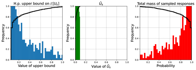
TriviaQA dataset

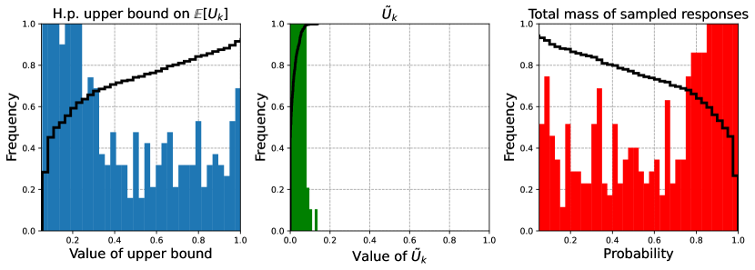
AmbigQA dataset

Figure 7: Distributions of bounds on the missing mass. The left figure for each dataset presents the empirical distribution of the upper bounds on the missing mass $\mathbb{E}[U_{k}]$. The middle figure presents the empirical distribution of $\tilde{U}_{k}$, the missing mass computed on a finite support approximation (where the support is obtained by taking samples from the LLM until a cumulative probability of 95% or 1000 samples are achieved). The right graph shows the empirical distribution of $P(\tilde{\mathcal{X}})$, the cumulative probabilities of all responses generated by the language model. For each figure, one observation (sample) corresponds to a single query. The black curves represent the corresponding empirical cumulative distribution functions for the upper bounds on $\mathbb{E}{U_{k}}$ and for $\tilde{U}_{k}$, and the empirical survival function (1 minus the empirical distribution function) for the distribution of $P(\tilde{\mathcal{X}})$.

References

- Angelopoulos et al. (2023) Anastasios N Angelopoulos, Stephen Bates, et al. Conformal prediction: A gentle introduction. Foundations and Trends® in Machine Learning, 16(4):494–591, 2023.
- Antorán et al. (2020) Javier Antorán, James Allingham, and José Miguel Hernández-Lobato. Depth uncertainty in neural networks. Conference on Neural Information Processing Systems (NeurIPS), 2020.
- Azaria and Mitchell (2023) Amos Azaria and Tom Mitchell. The internal state of an LLM knows when its lying. In Conference on Empirical Methods in Natural Language Processing (EMNLP), 2023.
- Berend and Kontorovich (2012) Daniel Berend and Aryeh Kontorovich. The missing mass problem. Statistics & Probability Letters, 82(6):1102–1110, 2012.
- Berend and Kontorovich (2013) Daniel Berend and Aryeh Kontorovich. On the concentration of the missing mass. Electronic Communications in Probability, 2013.
- Berend et al. (2017) Daniel Berend, Aryeh Kontorovich, and Gil Zagdanski. The expected missing mass under an entropy constraint. Entropy, 19(7):315, 2017.
- Blundell et al. (2015) Charles Blundell, Julien Cornebise, Koray Kavukcuoglu, and Daan Wierstra. Weight uncertainty in neural network. In International Conference on Machine Learing (ICML), 2015.
- Bubeck et al. (2023) Sébastien Bubeck, Varun Chandrasekaran, Ronen Eldan, Johannes Gehrke, Eric Horvitz, Ece Kamar, Peter Lee, Yin Tat Lee, Yuanzhi Li, Scott Lundberg, Harsha Nori, Hamid Palangi, Marco Tulio Ribeiro, and Yi Zhang. Sparks of artificial general intelligence: Early experiments with gpt-4. arXiv preprint arXiv:2303.12712, 2023.
- Burns et al. (2023) Collin Burns, Haotian Ye, Dan Klein, and Jacob Steinhardt. Discovering latent knowledge in language models without supervision. In International Conference on Learning Representations (ICLR), 2023.
- Chen et al. (2024) Chao Chen, Kai Liu, Ze Chen, Yi Gu, Yue Wu, Mingyuan Tao, Zhihang Fu, and Jieping Ye. INSIDE: LLMs’ internal states retain the power of hallucination detection. In International Conference on Learning Representations (ICLR), 2024.
- Cole et al. (2023) Jeremy R. Cole, Michael JQ Zhang, Daniel Gillick, Julian Martin Eisenschlos, Bhuwan Dhingra, and Jacob Eisenstein. Selectively answering ambiguous questions. In Conference on Empirical Methods in Natural Language Processing (EMNLP), 2023.
- Devlin et al. (2019) Jacob Devlin, Ming-Wei Chang, Kenton Lee, and Kristina Toutanova. BERT: Pre-training of deep bidirectional transformers for language understanding. arXiv preprint arXiv:1810.04805, 2019.
- Dwaracherla et al. (2023) Vikranth Dwaracherla, Zheng Wen, Ian Osband, Xiuyuan Lu, Seyed Mohammad Asghari, and Benjamin Van Roy. Ensembles for uncertainty estimation: Benefits of prior functions and bootstrapping. Transactions on Machine Learning Research (TMLR), 2023. ISSN 2835-8856.
- Fellbaum (1998) Christiane Fellbaum. WordNet: An electronic lexical database. MIT press, 1998.
- Gale and Sampson (1995) William A Gale and Geoffrey Sampson. Good-turing frequency estimation without tears. Journal of quantitative linguistics, 2(3):217–237, 1995.
- Gemini Team, Google (2023) Gemini Team, Google. Gemini: A family of highly capable multimodal models. arXiv preprint arXiv:2312.11805, 2023. [Online; accessed 01-February-2024].
- Hou et al. (2024) Bairu Hou, Yujian Liu, Kaizhi Qian, Jacob Andreas, Shiyu Chang, and Yang Zhang. Decomposing uncertainty for large language models through input clarification ensembling. In International Conference on Machine Learing (ICML), 2024.
- Jiang et al. (2024) Mingjian Jiang, Yangjun Ruan, Sicong Huang, Saifei Liao, Silviu Pitis, Roger Grosse, and Jimmy Ba. Calibrating language models via augmented prompt ensembles. In Workshop on Challenges in Deployable Generative AI at International Conference on Machine Learning, 2024.
- Johnson et al. (2024) Daniel D. Johnson, Daniel Tarlow, David Duvenaud, and Chris J. Maddison. Experts don’t cheat: Learning what you don’t know by predicting pairs. arXiv preprint arXiv:2402.08733, 2024.
- Joshi et al. (2017) Mandar Joshi, Eunsol Choi, Daniel S Weld, and Luke Zettlemoyer. TriviaQA: A large scale distantly supervised challenge dataset for reading comprehension. In Transactions of the Association for Computational Linguistics (ACL), pages 1601–1611, 2017.
- Kadavath et al. (2022) Saurav Kadavath, Tom Conerly, Amanda Askell, Tom Henighan, Dawn Drain, Ethan Perez, Nicholas Schiefer, Zac Hatfield Dodds, Nova DasSarma, Eli Tran-Johnson, and et al. Language models (mostly) know what they know. arXiv preprint arXiv:2207.05221, 2022.