Integrated density of states for the Poisson point interactions on $\mathbf{R}^{3}$

by

Masahiro Kaminaga111 Department of Information Technology, Tohoku Gakuin University, 3-1, Shimizu-Koji, Sendai 984-8588, Japan. E-mail: kaminaga@mail.tohoku-gakuin.ac.jp , Takuya Mine222 Faculty of Arts and Sciences, Kyoto Institute of Technology, Matsugasaki, Sakyo-ku, Kyoto 606-8585, Japan. E-mail: mine@kit.ac.jp , and Fumihiko Nakano333 Mathematical institute, Tohoku University, Sendai 980-8578, Japan. E-mail: fumihiko.nakano.e4@tohoku.ac.jp

Abstract

We determine the principal term of the asymptotics of the integrated density of states (IDS) $N(\lambda)$ for the Schrödinger operator with point interactions on $\mathbf{R}^{3}$ as $\lambda\to-\infty$, provided that the set of positions of the point obstacles is the Poisson configuration, and the interaction parameters are bounded i.i.d. random variables. In particular, we prove $N(\lambda)=O(|\lambda|^{-3/2})$ as $\lambda\to-\infty$. In the case that all interaction parameters are equal to a constant, we give a more detailed asymptotics of $N(\lambda)$, and verify the result by a numerical method using R.

1 Introduction

Let $Y$ be a set of points in $\mathbf{R}^{d}$ ($d=1,2,3$) without accumulation points in $\mathbf{R}^{d}$. Let $\alpha=(\alpha_{y})_{y\in Y}$ be a sequence of real numbers. We define the operator $-\Delta_{\alpha,Y}$ on $L^{2}(\mathbf{R}^{d})$ by

$\displaystyle-\Delta_{\alpha,Y}u:=$ $\displaystyle\ -\Delta|_{\mathbf{R}^{d}\setminus Y}u,$
$\displaystyle D(-\Delta_{\alpha,Y}):=$ $\displaystyle\ \{u\in L^{2}(\mathbf{R}^{d})\cap H^{2}_{\rm loc}(\mathbf{R}^{d}\setminus Y)\,;\,-\Delta|_{\mathbf{R}^{d}\setminus Y}u\in L^{2}(\mathbf{R}^{d}),$
$\displaystyle\qquad u\mbox{ satisfies }(BC)_{y}\mbox{ for every }y\in Y\},$

where $\Delta|_{\mathbf{R}^{d}\setminus Y}u=\sum_{j=1}^{d}\partial^{2}u/\partial x_{j}^{2}$ is defined as an element of the Schwartz distribution ${\cal D}^{\prime}(\mathbf{R}^{d}\setminus Y)$, and $D(H)$ is the domain of a linear operator $H$ (the notation $A:=B$ means that $A$ is defined by $B$). The boundary condition $(BC)_{y}$ at the point $y\in Y$ is defined as follows.

  • For $d=1$,

    $\displaystyle u(y-0)=u(y+0)=u(y),\quad u^{\prime}(y+0)-u^{\prime}(y-0)=\alpha_{y}u(y).$
  • For $d=2$,

    $\displaystyle u(x)=u_{y,0}\log|x-y|+u_{y,1}+o(1)\quad(x\to y),\quad 2\pi\alpha_{y}u_{y,0}+u_{y,1}=0.$
  • For $d=3$,

    $\displaystyle u(x)=u_{y,0}|x-y|^{-1}+u_{y,1}+o(1)\quad(x\to y),\quad-4\pi\alpha_{y}u_{y,0}+u_{y,1}=0.$

Here, $\displaystyle u(y\pm 0)=\lim_{\epsilon\to\pm 0}u(y\pm\epsilon)$, and $u_{y,0}$ and $u_{y,1}$ are constants.

It is known that the operator $-\Delta_{\alpha,Y}$ is self-adjoint on $L^{2}(\mathbf{R}^{d})$ under suitable conditions on $\alpha$ and $Y$, e.g., the uniform discreteness condition

$\displaystyle d_{*}:=\inf_{y,y^{\prime}\in Y,\ y\not=y^{\prime}}|y-y^{\prime}|>0$ (1)

(see e.g. [1]). Since the support of the interaction is concentrated on the set $Y$, the quantum system governed by the Hamiltonian $-\Delta_{\alpha,Y}$ is called ‘point interaction model’, ‘zero-range interaction model’, ‘delta interaction model’, or ‘Fermi pseudo potential model’, etc. The monograph by Albeverio et al. [1] contains most of the basic facts about the operator $-\Delta_{\alpha,Y}$, and references up to 2004.

Let us review known results about the random point interactions, that is, the case that $\alpha$ or $Y$ depends on some random parameter $\omega$. There are numerous results in the case $d=1$ (references are found in [15]). When $d=2$ or $3$, there are several results in the case $Y=\mathbf{Z}^{d}$ or its random subset, and $\alpha_{\omega}=(\alpha_{\omega,y})_{y\in\mathbf{Z}^{d}}$ are i.i.d. (independently, identically distributed) random variables. Albeverio–Høegh-Krohn–Kirsch–Martinelli [2] study the spectrum of $-\Delta_{\alpha_{\omega},\mathbf{Z}^{d}}$. Boutet de Monvel–Grinshpun [3] and Hislop–Kirsch–Krishna [7] prove the Anderson localization near the bottom of the spectrum. Recently Hislop–Kirsch–Krishna [8] study the eigenvalue statistics. Dorlas–Macris–Pulé [5] study the random point interactions on $\mathbf{R}^{2}$ in a constant magnetic field.

In the present paper, we consider the following case.

Assumption 1.
  1. (i)

    $Y_{\omega}$ is the Poisson configuration (the support of the Poisson point process measure) on $\mathbf{R}^{d}$ with intensity measure $\rho dx$ for some constant $\rho>0$.

  2. (ii)

    The parameters $\alpha_{\omega}=(\alpha_{\omega,y})_{y\in Y_{\omega}}$ are real-valued i.i.d. random variables with common distribution $\nu$ on $\mathbf{R}$. Moreover, $(\alpha_{\omega,y})_{y\in Y_{\omega}}$ are independent of $Y_{\omega}$.

We denote $H_{\omega}=-\Delta_{\alpha_{\omega},Y_{\omega}}$ in the sequel. For the definition of the Poisson point process, see Appendix (section 6.1). Under Assumption 1, the Schrödinger operator with random scalar potential

$\displaystyle-\Delta+\sum_{y\in Y_{\omega}}\alpha_{\omega,y}V_{0}(x-y)\quad(\mbox{$V_{0}$: scalar function})$ (2)

is a mathematical model which governs the motion of a quantum particle in an amorphous material, and is extensively studied in the theory of random Schrödinger operators (see e.g. [15]). Formally, the operator $-\Delta_{\alpha_{\omega},Y_{\omega}}$ is a special case of (2), in the case that $V_{0}$ is a zero-range potential. Notice that the condition (1) is not satisfied under Assumption 1. When $d=1$, the operator $H_{\omega}$ under Assumption 1 is studied by several authors ([6, 13, 12, 14]). Especially, the self-adjointness is proved in [14] (or it can be proved by an application of the deterministic result [11]). When $d=2$ or $3$, the operator $H_{\omega}$ under Assumption 1 is first studied recently by the authors [10]. Their results are summarized as follows.

Theorem 2 ([10]).

Let $d=1,2$ or $3$, and suppose Assumption 1 holds. Then, the following holds.

  1. (1)

    The operator $H_{\omega}$ is self-adjoint almost surely.

  2. (2)

    The spectrum $\sigma(H_{\omega})$ is given as follows. When $d=1$, we have

    $\displaystyle\sigma(H_{\omega})=\begin{cases}[0,\infty)&(\mathop{\rm supp}\nolimits\nu\subset[0,\infty)),\\ \mathbf{R}&(\mathop{\rm supp}\nolimits\nu\cap(-\infty,0)\not=\emptyset),\end{cases}$

    almost surely. When $d=2,3$, we have $\sigma(H_{\omega})=\mathbf{R}$ almost surely.

Next we introduce the integrated density of states. For a bounded open set $U$ in $\mathbf{R}^{d}$, let $-\Delta_{\alpha,Y,U}^{D}$ (resp. $-\Delta_{\alpha,Y,U}^{N}$) be the restriction of the operator $-\Delta_{\alpha,Y}$ to the set $U$ with Dirichlet boundary conditions (resp. Neumann boundary conditions) on the boundary $\partial U$. For $\lambda\in\mathbf{R}$ and $\#=D$ or $N$, let $N_{\alpha,Y,U}^{\#}(\lambda)$ be the number of the eigenvalues of $-\Delta_{\alpha,Y,U}^{\#}$ less than or equal to $\lambda$, counted with multiplicity. For $(\alpha_{\omega},Y_{\omega})$ satisfying Assumption 1, we define

$\displaystyle N^{\#}(\lambda):=$ $\displaystyle\ \lim_{L\to\infty}\frac{N_{\alpha_{\omega},Y_{\omega},Q_{L}}^{\#}(\lambda)}{|Q_{L}|}\quad(\#=D\mbox{ or }N),$ (3)

where $Q_{L}=(0,L)^{d}$ and $|E|$ is the Lebesgue measure of a Lebesgue measurable set $E$. Under Assumption 1, we can prove by an ergodicity argument that the RHS of (3) converges almost surely, and

$\displaystyle N^{\#}(\lambda)=$ $\displaystyle\ \lim_{L\to\infty}\frac{\mathbf{E}[N_{\alpha_{\omega},Y_{\omega},Q_{L}}^{\#}(\lambda)]}{|Q_{L}|}\quad(\#=D\mbox{ or }N),$ (4)

almost surely, where $\mathbf{E}[X]$ is the expectation of a random variable $X$. The equation (4) implies $N^{\#}(\lambda)$ is independent of $\omega$, almost surely. Furthermore, we can prove $N^{D}(\lambda)=N^{N}(\lambda)$ if either $N^{D}$ or $N^{N}$ is continuous at $\lambda$ (since $N^{\#}(\lambda)$ is monotone non-decreasing, this condition holds except at most countable points of $\mathbf{R}$). So we simply write $N(\lambda):=N^{D}(\lambda)=N^{N}(\lambda)$ and call this function the integrated density of states (IDS).

For $\lambda<0$, it is convenient to introduce another counting function

$\displaystyle N_{\alpha,Y}(\lambda):=$ $\displaystyle\ \#\{\mu\leq\lambda\,;\,\mu\mbox{ is an eigenvalue of }-\Delta_{\alpha,Y}\},$
$\displaystyle N_{\alpha,Y,U}(\lambda):=$ $\displaystyle\ N_{\alpha|_{Y\cap U},Y\cap U}(\lambda),$

where eigenvalues are counted with multiplicity, $\alpha|_{Y\cap U}$ is the restriction of the sequence $\alpha=(\alpha_{y})_{y\in Y}$ on the subset $Y\cap U$, and $\#S$ is the cardinality of a set $S$. Notice that the operator $-\Delta_{\alpha|_{Y\cap U},Y\cap U}$ is defined on $L^{2}(\mathbf{R}^{d})$ (not $L^{2}(U)$). We can prove that if $(\alpha_{\omega},Y_{\omega})$ satisfies Assumption 1, $\lambda<0$ and $N(\lambda)=N^{D}(\lambda)=N^{N}(\lambda)$, then

N(λ)=limLNαω,Yω,QL(λ)|QL|𝑁𝜆subscript𝐿subscript𝑁subscript𝛼𝜔subscript𝑌𝜔subscript𝑄𝐿𝜆subscript𝑄𝐿\displaystyle N(\lambda)=\lim_{L\to\infty}\frac{N_{\alpha_{\omega},Y_{\omega},Q_{L}}(\lambda)}{|Q_{L}|} (5)

almost surely (Lemma 13). The advantage of the new expression (5) is that $N_{\alpha_{\omega},Y_{\omega},Q_{L}}(\lambda)$ can be calculated explicitly (Proposition 11).

The asymptotics of IDS near the bottom of the spectrum is intensively studied in the theory of random Schrödinger operators (see e.g. [15]). In the present paper, we give an asymptotic formula of IDS $N(\lambda)$ for our operator $H_{\omega}$ as $\lambda\to-\infty$ in the case $d=3$, under Assumption 1.

First we consider the case $\alpha_{\omega}=(\alpha_{\omega,y})_{y\in Y_{\omega}}$ is a constant sequence, that is, $\alpha_{\omega,y}$ is equal to a deterministic value independent of $\omega$ and $y$. We denote its common value by $\alpha$, and write $-\Delta_{\alpha,Y_{\omega}}:=-\Delta_{\alpha_{\omega},Y_{\omega}}$ for simplicity. In order to state our main result, we introduce some auxiliary functions. If $s>\mathop{\rm max}\limits(0,-4\pi\alpha)$, it is easy to see that the equation with respect to $R$

$\displaystyle s-\frac{e^{-sR}}{R}=-4\pi\alpha$ (6)

has a unique positive solution $R$, which we denote by $R_{\alpha}(s)$. We denote the inverse function of $R=R_{\alpha}(s)$ by $s=s_{\alpha}(R)$. Particularly when $\alpha=0$, the equation (6) becomes a simple equation $sR-e^{-sR}=0$. We denote the unique positive solution of $t-e^{-t}=0$ by $t_{0}(\doteqdot 0.567...$). Then we have explicitly

$\displaystyle R_{0}(s)=\frac{t_{0}}{s},\quad s_{0}(R)=\frac{t_{0}}{R}.$

For $\alpha\not=0$, we still have

$\displaystyle R_{\alpha}(s)\sim\frac{t_{0}}{s}\quad(s\to\infty),\quad s_{\alpha}(R)\sim\frac{t_{0}}{R}\quad(R\to+0),$ (7)

where $f\sim g$ means $f/g\to 1$ (Proposition 5). The function $R_{\alpha}(s)$ can be explicitly computed with the aid of some numerical tool.

Theorem 3.

Let $d=3$. Suppose that $\alpha_{\omega}$ and $Y_{\omega}$ satisfy Assumption 1. Suppose further that $\alpha_{\omega}$ is a constant sequence with its common value $\alpha$. Let $N(\lambda)$ be the corresponding IDS for the operator $H_{\omega}=-\Delta_{\alpha,Y_{\omega}}$. Then, for any $\epsilon$ with $0<\epsilon<3$, we have

$\displaystyle N(-s^{2})=\frac{2\pi}{3}\rho^{2}R_{\alpha}(s)^{3}+O(s^{-6+\epsilon})\quad(s\to\infty).$ (8)

In particular, the principal term of the asymptotics is given by

$\displaystyle N(-s^{2})\sim\frac{2\pi}{3}\rho^{2}t_{0}^{3}s^{-3}\quad(s\to\infty).$ (9)

In section 5, we give a numerical verification of Theorem 3, using R.

Next we consider the case that $\mathop{\rm supp}\nolimits\nu$ is bounded, i.e., there exist constants $\alpha_{-}$ and $\alpha_{+}$ such that $\alpha_{-}\leq\alpha_{\omega,y}\leq\alpha_{+}$ for every $y\in Y_{\omega}$, almost surely. By the monotonicity of the negative eigenvalues of $-\Delta_{\alpha,Y}$ with respect to $\alpha$ ((1) of Proposition 12), we have

$\displaystyle N_{\alpha_{-},Y_{\omega},U}(\lambda)\geq N_{\alpha_{\omega},Y_{\omega},U}(\lambda)\geq N_{\alpha_{+},Y_{\omega},U}(\lambda)$

for every $\lambda<0$ and every bounded open set $U$, almost surely. Since the principal term of the asymptotics (9) is independent of $\alpha$, we have the following corollary.

Corollary 4.

Let $d=3$. Suppose that $\alpha_{\omega}$ and $Y_{\omega}$ satisfy Assumption 1, and $\mathop{\rm supp}\nolimits\nu$ is bounded. Then, we have the asymptotics

$\displaystyle N(-s^{2})\sim\frac{2\pi}{3}\rho^{2}t_{0}^{3}s^{-3}\quad(s\to\infty).$ (10)

Let us compare the asymptotics (10) with the corresponding result for the scalar type Poisson random potential

$\displaystyle-\Delta+\sum_{y\in Y_{\omega}}V_{0}(x-y),$ (11)

where $V_{0}$ is a real-valued function and $Y_{\omega}$ is the Poisson configuration. If $V_{0}\leq 0$, $V_{0}$ has global minimum at $x=0$, and $V_{0}$ satisfies some regularity and decaying conditions, Pastur [15, Theorem 9.4] shows

$\displaystyle\log N(\lambda)=-\frac{|\lambda|}{|V_{0}(0)|}\log|\lambda|\cdot(1+o(1))\quad(\lambda\to-\infty).$ (12)

The asymptotics (12) implies $N(\lambda)$ decays super-exponentially, much faster than the polynomial decay (10).

Heuristically, the asymptotics (12) is explained as follows. If the operator (11) has a bound state localized near a point $a$ with negative energy $\lambda$, there must be a potential well of depth $|\lambda|$ near the point $a$. Thus it is necessary that at least

$\displaystyle n=\left[\frac{|\lambda|}{|V_{0}(0)|}\right]$ (13)

points of $Y_{\omega}$ are in the ball of small radius $\epsilon$ centered at $a$, where $[x]$ is the greatest integer less than or equal to $x$. The probability of this event is

$\displaystyle\frac{(\rho|B_{\epsilon}(0)|)^{n}}{n!}e^{-\rho|B_{\epsilon}(0)|},$ (14)

where $B_{\epsilon}(0)$ is a ball of radius $\epsilon$ centered at the origin. Then, roughly speaking, the asymptotics (12) is deduced from (13), (14), and the Stirling formula

$\displaystyle n!\sim(2\pi n)^{1/2}\left({n}/{e}\right)^{n}\quad(n\to\infty).$

In the case of point interactions, the situation is completely different. Consider the case $Y=\{y_{1},y_{2}\}$ is a two-point set, and $\alpha$ is a constant sequence. Then, by an explicit calculation, we can prove that the operator $-\Delta_{\alpha,Y}$ has a negative eigenvalue $\lambda=-(s_{\alpha}(R))^{2}$ for small $R$ (section 2), and $s_{\alpha}(R)\to\infty$ as $R\to 0$ by (7). Thus the asymptotics of $N(\lambda)$ is determined from the number of pairs of points in $Y_{\omega}$ close to each other (Lemma 7). The expectation of the number of such pairs can be explicitly computed (Proposition 6), and we obtain the above result.

The present paper is organized as follows. In section 2, we review the results about the spectrum of $-\Delta_{\alpha,Y}$ when $\#Y=1,2$. In section 3, we calculate the expectation of the number of $n$-point clusters in the Poisson configuration. In section 4, we prove Theorem 3. In section 5, we give a numerical verification of Theorem 3, using R. In Appendix (section 6), we review some known results about the Poisson point process, spectrum of the Hamiltonian with point interactions, and the operator norm of a matrix operator.

2 Spectrum of the Hamiltonian with one or two point interactions

Let $d=3$, $Y$ be a finite set in $\mathbf{R}^{3}$, and $\alpha=(\alpha_{y})_{y\in Y}$ be a sequence of real numbers. Put $N:=\#Y$. It is known that

$\displaystyle\ \sigma(-\Delta_{\alpha,Y})=\sigma_{p}(-\Delta_{\alpha,Y})\cup[0,\infty),$
$\displaystyle\ \sigma_{p}(-\Delta_{\alpha,Y})\subset(-\infty,0],$

where $\sigma_{p}(-\Delta_{\alpha,Y})$ is the point spectrum of $-\Delta_{\alpha,Y}$ (see [1] or Proposition 11 in Appendix). More explicitly, $\sigma_{p}(-\Delta_{\alpha,Y})$ for $N=1,2$ is given as follows.

When $N=1$, Proposition 11 implies that $-s^{2}$ ($s>0$) is an eigenvalue of $-\Delta_{\alpha,Y}$ if and only if

$\displaystyle\alpha+\frac{s}{4\pi}=0.$

Then we see that

$\displaystyle\sigma_{p}(-\Delta_{\alpha,Y})\cap(-\infty,0)=\begin{cases}\emptyset&(\alpha\geq 0),\\ \{-(4\pi\alpha)^{2}\}&(\alpha<0).\end{cases}$

When $N=2$, $Y=\{y_{1},y_{2}\}$, $\alpha_{y_{1}}=\alpha_{y_{2}}=\alpha$, and $R:=|y_{1}-y_{2}|>0$, Proposition 11 implies that $-s^{2}$ ($s>0$) is an eigenvalue of $-\Delta_{\alpha,Y}$ if and only if

$\displaystyle\left|\begin{matrix}\displaystyle\alpha+\frac{s}{4\pi}&\displaystyle-\frac{e^{-sR}}{4\pi R}\\[8.53581pt] \displaystyle-\frac{e^{-sR}}{4\pi R}&\displaystyle\alpha+\frac{s}{4\pi}\end{matrix}\right|=0\Leftrightarrow\left(\alpha+\frac{s}{4\pi}\right)^{2}-\left(\frac{e^{-sR}}{4\pi R}\right)^{2}=0.$

This equation is satisfied if and only if

$\displaystyle s+\frac{e^{-sR}}{R}=-4\pi\alpha$ (15)

or

$\displaystyle s-\frac{e^{-sR}}{R}=-4\pi\alpha.$ (16)

The solution $s$ to the equation (15) does not exist if $\alpha\geq 0$, and is bounded by $-4\pi\alpha$ if $\alpha<0$. The equation (16) is the same as (6), and the solution is equal to $s_{\alpha}(R)$ by definition. An asymptotics of $s_{\alpha}(R)$ and that of its inverse $R_{\alpha}(s)$ are given as follows.

Proposition 5.

Let $t_{0}$ be the unique positive solution of $t-e^{-t}=0$.

  1. (1)

    Suppose $\alpha=0$. Then we have $s_{0}(R)=t_{0}/R$ and $R_{0}(s)=t_{0}/s$.

  2. (2)

    Suppose $\alpha\not=0$. Then, for any $\epsilon>0$, there exists a positive constant $R_{0}$ dependent on $\alpha$ and $\epsilon$ such that

    $\displaystyle\frac{t_{0}-\epsilon}{R}<s_{\alpha}(R)<\frac{{t_{0}+\epsilon}}{R}$ (17)

    for any $R$ with $0<R<R_{0}$, and

    $\displaystyle\frac{t_{0}-\epsilon}{s}<R_{\alpha}(s)<\frac{t_{0}+\epsilon}{s}$ (18)

    for any $s$ with $s>(t_{0}+\epsilon)/R_{0}$.

Proof.

The proof of (1) is already given in the introduction. We prove (2). Let $\phi(t):=t-e^{-t}$. Then the defining equation (6) of $s_{\alpha}(R)$ is equivalent to

$\displaystyle\phi(sR)+4\pi\alpha R=0.$ (19)

Since

$\displaystyle\ \frac{\partial\phi}{\partial t}=1+e^{-t}>0,$
$\displaystyle\ \lim_{s\to+0}\phi(sR)=-1,\quad\lim_{s\to\infty}\phi(sR)=\infty,$

we see that the left hand side of (19) is monotone increasing with respect to $s$, and (19) has a unique positive solution $s_{\alpha}(R)$ if $-1+4\pi\alpha R<0$. Since $\phi(t_{0})=0$ by definition, we have $\phi(t_{0}-\epsilon)<0<\phi(t_{0}+\epsilon)$ for $\epsilon>0$, and

$\displaystyle\ \phi\left(t_{0}-\epsilon\right)+4\pi\alpha R<0,$
$\displaystyle\ \phi\left(t_{0}+\epsilon\right)+4\pi\alpha R>0$

for small $R>0$. So the left hand side of (19) is negative for $s=(t_{0}-\epsilon)/R$, is positive for $s=(t_{0}+\epsilon)/R$, if $R$ is sufficiently small. Thus (17) follows from the intermediate value theorem. Then we immediately have (18), since $R=R_{\alpha}(s)$ is the inverse function of $s=s_{\alpha}(R)$. ∎

3 Number of clusters in Poisson configuration

Let us calculate the expectation of the number of $n$-point clusters in the Poisson configuration in $\mathbf{R}^{d}$ ($d=1,2,3,\ldots$). For $y\in\mathbf{R}^{d}$ and $R>0$, let $B_{y}(R):=\{z\in\mathbf{R}^{d};|z-y|<R\}$. For the Poisson configuration $Y_{\omega}$ in $\mathbf{R}^{d}$, we put

$\displaystyle n_{y}(R):=\#(Y_{\omega}\cap B_{y}(R)).$ (20)
Proposition 6.

Let $Y_{\omega}$ be the Poisson configuration with intensity $\rho dx$, where $\rho$ is a positive constant. Let $L>0$ and put $Q_{L}:=[0,L]^{d}$. Then, we have for $n=1,2,3,\ldots$

$\displaystyle\frac{\mathbf{E}[\#\{y\in Y_{\omega}\cap Q_{L}\,;\,n_{y}(R)=n\}]}{|Q_{L}|}=\frac{1}{(n-1)!}|B_{0}(R)|^{n-1}\rho^{n}e^{-\rho|B_{0}(R)|}.$ (21)
Proof.

Let $Q_{L}^{\prime}=[-R,L+R]^{d}$. If $y\in Q_{L}$, then $B_{y}(R)\subset Q_{L}^{\prime}$. Moreover, $Y_{\omega}\cap Q_{L}^{\prime}$ and $Y_{\omega}\cap(Q_{L}^{\prime})^{c}$ are independently distributed. So we can replace $Y_{\omega}$ in the definition of $n_{y}(R)$ by $Y_{\omega}^{\prime}:=Y_{\omega}\cap Q_{L}^{\prime}$, when we calculate LHS of (21). Then,

$\displaystyle\ \mathbf{E}[\#\{y\in Y_{\omega}\cap Q_{L}\,;\,n_{y}(R)=n\}]$
$\displaystyle=$ $\displaystyle\ \sum_{k=n}^{\infty}\mathbf{E}[\#\{y\in Y_{\omega}\cap Q_{L}\,;\,n_{y}(R)=n\}\mid\#Y_{\omega}^{\prime}=k]\cdot\mathbf{P}(\#Y_{\omega}^{\prime}=k),$

where $\mathbf{E}[A|B]$ is the conditional expectation of $A$ under the condition $B$. Under the condition $\#Y_{\omega}^{\prime}=k$, the points $Y_{\omega}^{\prime}=\{y_{1},\ldots,y_{k}\}$ obey independent uniform distributions on $Q_{L}^{\prime}$ (Proposition 9). Thus we have an expression about the conditional probability

$\displaystyle\ \mathbf{P}(y_{j}\in Q_{L},\ n_{y_{j}}(R)=n\mid\#Y_{\omega}^{\prime}=k)$
$\displaystyle=$ $\displaystyle\ \frac{|Q_{L}|}{|Q_{L}^{\prime}|}\cdot\frac{(k-1)!}{(n-1)!(k-n)!}\cdot\left(\frac{|B_{y_{j}}(R)|}{|Q_{L}^{\prime}|}\right)^{n-1}\cdot\left(\frac{|Q_{L}^{\prime}|-|B_{y_{j}}(R)|}{|Q_{L}^{\prime}|}\right)^{k-n}$

for $j=1,\ldots,k$. Then

$\displaystyle\ \mathbf{E}[\#\{y\in Y_{\omega}\cap Q_{L}\,;\,n_{y}(R)=n\}]$
$\displaystyle=$ $\displaystyle\ \sum_{k=n}^{\infty}\sum_{j=1}^{k}\mathbf{P}(y_{j}\in Q_{L},\ n_{y_{j}}(R)=n\mid\#Y_{\omega}^{\prime}=k)\cdot\mathbf{P}(\#Y_{\omega}^{\prime}=k)$
$\displaystyle=$ $\displaystyle\ \sum_{k=n}^{\infty}k\cdot\frac{|Q_{L}|}{|Q_{L}^{\prime}|}\cdot\frac{(k-1)!}{(n-1)!(k-n)!}\cdot\left(\frac{|B_{0}(R)|}{|Q_{L}^{\prime}|}\right)^{n-1}\cdot\left(\frac{|Q_{L}^{\prime}|-|B_{0}(R)|}{|Q_{L}^{\prime}|}\right)^{k-n}$
$\displaystyle\qquad\cdot\frac{(\rho|Q_{L}^{\prime}|)^{k}}{k!}e^{-\rho|Q_{L}^{\prime}|}$
$\displaystyle=$ $\displaystyle\ \frac{|Q_{L}||B_{0}(R)|^{n-1}}{(n-1)!}e^{-\rho|Q_{L}^{\prime}|}\sum_{k=n}^{\infty}\frac{\rho^{k}(|Q_{L}^{\prime}|-|B_{0}(R)|)^{k-n}}{(k-n)!}$
$\displaystyle=$ $\displaystyle\ \frac{|Q_{L}||B_{0}(R)|^{n-1}}{(n-1)!}e^{-\rho|Q_{L}^{\prime}|}\rho^{n}e^{\rho(|Q_{L}^{\prime}|-|B_{0}(R)|)}$
$\displaystyle=$ $\displaystyle\ \frac{|Q_{L}||B_{0}(R)|^{n-1}}{(n-1)!}\rho^{n}e^{-\rho|B_{0}(R)|}.$

Remark. This result can also be deduced by Palm distribution; see section 6.2.

4 Proof of Theorem 3

In this section, we always suppose the assumptions in Theorem 3 hold, and prove Theorem 3. The relation between asymptotics of IDS and the number of 2-point clusters is given in the following lemma.

Lemma 7.

For every $\delta$ with $1/2<\delta<1$, and for every $m>0$, there exist constants $R_{0}=R_{0}(\rho,\alpha,\delta,m)>0$ and $C=C(\rho,\alpha,\delta,m)>0$ such that

$\displaystyle\mathbf{E}[N_{\alpha_{\omega},Y_{\omega},Q_{L}}(-(s_{\alpha}(R)-R^{m})^{2})]$
$\displaystyle\geq$ $\displaystyle\ \frac{1}{2}\mathbf{E}[\#\{y\in Y_{\omega}\cap Q_{L}\,;\,n_{y}(R)=2\}]-CR^{6\delta}|Q_{L}|,$ (22)
$\displaystyle\mathbf{E}[N_{\alpha_{\omega},Y_{\omega},Q_{L}}(-(s_{\alpha}(R)+R^{m})^{2})]$
$\displaystyle\leq$ $\displaystyle\ \frac{1}{2}\mathbf{E}[\#\{y\in Y_{\omega}\cap Q_{L}\,;\,n_{y}(R)=2\}]+CR^{6\delta}|Q_{L}|,$ (23)

for every $0<R<R_{0}$ and every $L>R^{-2}$, where $n_{y}(R)$ is defined in (20).

First we show that Lemma 7 implies Theorem 3.

Proof of Theorem 3.

Assume Lemma 7 holds. We make a change of variable $s=s_{\alpha}(R)-R^{m}$ in (22). Then we have by the Taylor theorem

$\displaystyle\ s_{\alpha}(R)=s+R^{m}$
$\displaystyle\Leftrightarrow$ $\displaystyle\ R=R_{\alpha}(s+R^{m})=R_{\alpha}(s)+\frac{dR_{\alpha}}{ds}(s+\theta R^{m})R^{m},\quad 0<\theta<1.$ (24)

Differentiating the defining equation of $R_{\alpha}$

$\displaystyle s-\frac{e^{-sR_{\alpha}}}{R_{\alpha}}=-4\pi\alpha$

with respect to $s$, we have

$\displaystyle\ 1+e^{-sR_{\alpha}}+\frac{(sR_{\alpha}+1)e^{-sR_{\alpha}}}{R_{\alpha}^{2}}\frac{dR_{\alpha}}{ds}=0$
$\displaystyle\Leftrightarrow$ $\displaystyle\ \frac{dR_{\alpha}}{ds}=-\frac{1+e^{-sR_{\alpha}}}{(sR_{\alpha}+1)e^{-sR_{\alpha}}}R_{\alpha}^{2}.$ (25)

By Proposition 5, we see that $s_{\alpha}(R)\sim t_{0}/R$ ($R\to 0$) and $R_{\alpha}(s)\sim t_{0}/s$ ($s\to\infty$). Then there exist positive constants $C_{1}$, $C_{2}$, $C_{3}$, $C_{4}$ such that

$\displaystyle\frac{C_{1}}{R}\leq s+\theta R^{m}\leq\frac{C_{2}}{R},$
$\displaystyle C_{3}R\leq R_{\alpha}(s+\theta R^{m})\leq C_{4}R$

for every $0\leq\theta\leq 1$ and small $R>0$. Thus (24) and (25) imply

$\displaystyle R=R_{\alpha}(s)+O(R^{m+2})=R_{\alpha}(s)(1+O(R^{m+1}))\quad(R\to 0).$ (26)

Take $m\geq 2$. Then, by (22), (26) and Proposition 6

$\displaystyle\frac{\mathbf{E}[N_{\alpha_{\omega},Y_{\omega},Q_{L}}(-s^{2})]}{|Q_{L}|}\geq$ $\displaystyle\ \frac{2\pi}{3}R^{3}\rho^{2}(1+O(R^{3}))-CR^{6\delta}$
$\displaystyle\geq$ $\displaystyle\ \frac{2\pi\rho^{2}}{3}R_{\alpha}(s)^{3}-C^{\prime}s^{-6\delta}$

for some $C^{\prime}>0$, and sufficiently large $s$ and $L$. Similarly, by a change of variable $s=s_{\alpha}(R)+R^{m}$, we have from (23) and Proposition 6

$\displaystyle\frac{\mathbf{E}[N_{\alpha_{\omega},Y_{\omega},Q_{L}}(-s^{2})]}{|Q_{L}|}\leq$ $\displaystyle\ \frac{2\pi\rho^{2}}{3}R_{\alpha}(s)^{3}+C^{\prime\prime}s^{-6\delta}$

for some $C^{\prime\prime}>0$, and sufficiently large $s$ and $L$. Taking the limit $L\to\infty$, we have the conclusion of Theorem 3. ∎

Proof of Lemma 7.

Take $\delta$ with $1/2<\delta<1$. Consider the decomposition $Y_{\omega}\cap Q_{L}=\widetilde{Y_{\omega}}\cup Z_{\omega}$, where

$\displaystyle Z_{\omega}=\{y\in Y_{\omega}\cap Q_{L}\mid n_{y}(R^{\delta})\geq 3\},\quad\widetilde{Y_{\omega}}=(Y_{\omega}\cap Q_{L})\setminus Z_{\omega}.$

In the sequel, we often omit the subscript $\omega$ and write $Y=Y_{\omega}$, etc. For the counting function, we also omit $Q_{L}$ and write $N_{\alpha_{\omega},Y_{\omega},Q_{L}}(\lambda)=N_{\alpha,Y}(\lambda)$, etc. By the properties of counting functions (Proposition 12), we have for $\lambda<0$

$\displaystyle\ N_{\alpha,\widetilde{Y}}(\lambda)\leq N_{\alpha,Y}(\lambda)\leq N_{\alpha,\widetilde{Y}}(\lambda)+\#Z,$
$\displaystyle\ \mathbf{E}[N_{\alpha,\widetilde{Y}}(\lambda)]\leq\mathbf{E}[N_{\alpha,Y}(\lambda)]\leq\mathbf{E}[N_{\alpha,\widetilde{Y}}(\lambda)]+\mathbf{E}[\#Z].$ (27)

By Proposition 6,

$\displaystyle\mathbf{E}[\#Z]=$ $\displaystyle\ \sum_{n=3}^{\infty}\frac{1}{(n-1)!}|B_{0}(R^{\delta})|^{n-1}\rho^{n}e^{-\rho|B_{0}(R^{\delta})|}|Q_{L}|$
$\displaystyle=$ $\displaystyle\ O(R^{6\delta})|Q_{L}|\quad(R\to 0).$ (28)

Next, we put for $y\in\widetilde{Y}$

$\displaystyle\widetilde{n_{y}}(R^{\delta}):=\#(\widetilde{Y}\cap B_{y}(R^{\delta})),$

then $1\leq\widetilde{n_{y}}(R^{\delta})\leq n_{y}(R^{\delta})\leq 2$ since $\widetilde{Y}\subset Y$. Thus we have another decomposition $\widetilde{Y}=\widetilde{Y}^{(1)}\cup\widetilde{Y}^{(2)}$, where

$\displaystyle\ \widetilde{Y}^{(j)}=\{y\in\widetilde{Y}\mid\widetilde{n_{y}}(R^{\delta})=j\}\quad(j=1,2).$

Then, for any $y\in\widetilde{Y}^{(2)}$, there exists a $y^{\prime}\in\widetilde{Y}^{(2)}$ such that $0<|y-y^{\prime}|<R^{\delta}$. This $y^{\prime}$ is unique, since otherwise we have $\widetilde{n_{y}}(R^{\delta})\geq 3$. Thus we can number the elements of $\widetilde{Y}^{(2)}$ and $\widetilde{Y}^{(1)}$ as

$\displaystyle\widetilde{Y}^{(2)}=$ $\displaystyle\ \{y_{1},y_{2}\}\cup\{y_{3},y_{4}\}\cup\cdots\cup\{y_{2n-1},y_{2n}\},$
$\displaystyle\ 0<|y_{1}-y_{2}|\leq|y_{3}-y_{4}|\leq\cdots\leq|y_{2n-1}-y_{2n}|<R^{\delta},$
$\displaystyle\widetilde{Y}^{(1)}=$ $\displaystyle\ \{y_{2n+1},\ldots,y_{2n+p}\},$

where $2n=\#\widetilde{Y}^{(2)}$ and $p=\#\widetilde{Y}^{(1)}$. By definition, we have

$\displaystyle|y_{k}-y_{k^{\prime}}|\geq R^{\delta},$

if $\{k,k^{\prime}\}\not=\{2j-1,2j\}$ for any $j=1,\ldots,n$.

Let $A$ and $B$ be $(2n+p)\times(2n+p)$ matrices given by

$\displaystyle\ A=\alpha I_{2n+p}+\frac{1}{4\pi}B,$
$\displaystyle\ B=(b_{jk}),\quad b_{jk}=\begin{cases}s&(j=k)\\ -\frac{e^{-s|y_{j}-y_{k}|}}{|y_{j}-y_{k}|}&(j\not=k),\end{cases}$

where $I_{m}$ is the identity matrix of degree $m$. For $j=1,\ldots,2n+p$, let $\mu_{j}=\mu_{j}(s)$ be the $j$-th smallest eigenvalue of $A$, counted with multiplicity. By Proposition 11, $\lambda=-s^{2}$ ($s>0$) is an eigenvalue of $-\Delta_{\alpha,\widetilde{Y}}$ if and only if $\mu_{j}(s)=0$ for some $j$.

We introduce another matrix $B^{\prime}$ given by

$\displaystyle B^{\prime}=(b^{\prime}_{jk}),\quad b^{\prime}_{jk}=\begin{cases}b_{jk}&(|y_{j}-y_{k}|<R^{\delta}),\\ 0&(|y_{j}-y_{k}|\geq R^{\delta}).\end{cases}$

Then the matrix $B^{\prime}$ is written as the direct sum

$\displaystyle\ B^{\prime}=\bigoplus_{j=1}^{n}B_{j}\oplus sI_{p},\quad B_{j}=\begin{pmatrix}s&-\frac{e^{-s|y_{2j-1}-y_{2j}|}}{|y_{2j-1}-y_{2j}|}\\ -\frac{e^{-s|y_{2j-1}-y_{2j}|}}{|y_{2j-1}-y_{2j}|}&s\end{pmatrix}.$

Put $A^{\prime}=\alpha I_{2n+p}+\frac{1}{4\pi}B^{\prime}$. Then, the $j$-th smallest eigenvalue $\mu^{\prime}_{j}=\mu^{\prime}_{j}(s)$ of $A^{\prime}$ is given explicitly as

$\displaystyle\ \mu^{\prime}_{j}=\alpha+\frac{1}{4\pi}\left(s-\frac{e^{-s|y_{2j-1}-y_{2j}|}}{|y_{2j-1}-y_{2j}|}\right)\quad(1\leq j\leq n),$ (29)
$\displaystyle\ \mu^{\prime}_{n+j}=\alpha+\frac{s}{4\pi}\quad(1\leq j\leq p),$
$\displaystyle\ \mu^{\prime}_{2n+p+1-j}=\alpha+\frac{1}{4\pi}\left(s+\frac{e^{-s|y_{2j-1}-y_{2j}|}}{|y_{2j-1}-y_{2j}|}\right)\quad(1\leq j\leq n).$

By the min-max principle, the difference of $\mu_{j}$ and $\mu_{j}^{\prime}$ is estimated as

$\displaystyle|\mu_{j}-\mu_{j}^{\prime}|\leq\|A-A^{\prime}\|=\frac{1}{4\pi}\|B-B^{\prime}\|,$ (30)

where $\|\cdot\|$ is the operator norm on $\ell^{2}(\widetilde{Y})\simeq\mathbf{C}^{2n+p}$. The components of the matrix $B-B^{\prime}$ are given as

$\displaystyle b_{jk}-b_{jk}^{\prime}=\begin{cases}0&(|y_{j}-y_{k}|<R^{\delta}),\\ -\frac{e^{-s|y_{j}-y_{k}|}}{|y_{j}-y_{k}|}&(|y_{j}-y_{k}|\geq R^{\delta}).\end{cases}$

By Proposition 14, we have

$\displaystyle\|B-B^{\prime}\|\leq\mathop{\rm max}\limits_{j}\sum_{k;|y_{j}-y_{k}|\geq R^{\delta}}\frac{e^{-s|y_{j}-y_{k}|}}{|y_{j}-y_{k}|}.$ (31)

In order to estimate the RHS of (31), we fix $y_{j}$, divide $\mathbf{R}^{3}$ into cubes of side $\widetilde{R_{\delta}}:=R^{\delta}/\sqrt{3}$, and classify the cubes into infinite layers, like Figure 1.
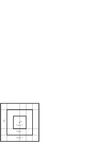
Refer to caption
Figure 1: Division by cubes of side $\widetilde{R_{\delta}}$

The diameter of each cube is $R^{\delta}$. By the construction of $\widetilde{Y}$, we see that

  1. (i)

    there is no point $y_{k}$ of $\widetilde{Y}$ with $|y_{j}-y_{k}|\geq R^{\delta}$ in Layer 0,

  2. (ii)

    there are at most two points of $\widetilde{Y}$ in each cube in Layer $\ell$ ($\ell\geq 1$),

  3. (iii)

    the minimal distance from $y_{j}$ to Layer $\ell$ is $\ell\widetilde{R_{\delta}}$,

  4. (iv)

    the number of cubes in Layer $\ell$ is

    $\displaystyle(2\ell+2)^{3}-(2\ell)^{3}=8(3\ell^{2}+3\ell+1)\leq 56\ell^{2}\quad(\ell\geq 1).$

The function $e^{-sR}/R$ is monotone decreasing with respect to $R$. Thus we have by (31) and (30)

$\displaystyle\|B-B^{\prime}\|\leq$ $\displaystyle\ \sum_{\ell=1}^{\infty}2\cdot 56\ell^{2}\cdot\frac{e^{-s\ell\widetilde{R_{\delta}}}}{\ell\widetilde{R_{\delta}}}=\frac{112}{\widetilde{R_{\delta}}}\sum_{\ell=1}^{\infty}\ell e^{-s\ell\widetilde{R_{\delta}}}=\frac{112}{\widetilde{R_{\delta}}}\frac{e^{-s\widetilde{R_{\delta}}}}{(1-e^{-s\widetilde{R_{\delta}}})^{2}},$
$\displaystyle\|A-A^{\prime}\|\leq$ $\displaystyle\ \frac{28}{\pi\widetilde{R_{\delta}}}\frac{e^{-s\widetilde{R_{\delta}}}}{(1-e^{-s\widetilde{R_{\delta}}})^{2}},$ (32)

where we used the formula

$\displaystyle\sum_{\ell=1}^{\infty}\ell e^{-\ell x}=\frac{e^{-x}}{(1-e^{-x})^{2}}\quad(x>0).$

By (30) and (32), we have

$\displaystyle\mu_{j}^{\prime}-g(s)\leq\mu_{j}\leq\mu_{j}^{\prime}+g(s),\quad g(s):=\frac{28}{\pi\widetilde{R_{\delta}}}\frac{e^{-s\widetilde{R_{\delta}}}}{(1-e^{-s\widetilde{R_{\delta}}})^{2}}.$ (33)

Let

$\displaystyle\ q^{\prime}=q_{\omega}^{\prime}:=\frac{1}{2}\#\{y\in\widetilde{Y_{\omega}}\,;\,\widetilde{n_{y}}(R)=2\},$
$\displaystyle\ \widetilde{n_{y}}(R)=\#(\widetilde{Y_{\omega}}\cap B_{y}(R)).$

If $0<R<1$, then $R<R^{\delta}$, and we have

$\displaystyle\ |y_{1}-y_{2}|\leq|y_{3}-y_{4}|\leq\cdots\leq|y_{2q^{\prime}-1}-y_{2q^{\prime}}|<R,$ (34)

and

$\displaystyle|y_{k}-y_{k^{\prime}}|\geq R$ (35)

if $\{k,k^{\prime}\}\not=\{2j-1,2j\}$ for any $j=1,\ldots,q^{\prime}$.

We shall show

$\displaystyle\mu_{j}(s_{\alpha}(R)-R^{m})<0\quad(j=1,\ldots,q^{\prime})$ (36)

for $m>0$ and sufficiently small $R$. To see this, we put $h(s,r)=s-e^{-sr}/r$. By (29) and (33),

$\displaystyle\ \mu_{j}(s_{\alpha}(R)-R^{m})$
$\displaystyle\leq$ $\displaystyle\ \alpha+\frac{1}{4\pi}h\bigl{(}s_{\alpha}(R)-R^{m},|y_{2j-1}-y_{2j}|\bigr{)}+g(s_{\alpha}(R)-R^{m}).$ (37)

Since

$\displaystyle\ \frac{\partial h}{\partial r}=\frac{(sr+1)e^{-sr}}{r^{2}}>0,$ (38)
$\displaystyle\ 1<\frac{\partial h}{\partial s}=1+e^{-sr}<2,\quad-r<\frac{\partial^{2}h}{\partial s^{2}}=-re^{-sr}<0,$ (39)

we have by (34), (38), (39), the Taylor theorem, and the definition of $s_{\alpha}(R)$,

$\displaystyle\ \alpha+\frac{1}{4\pi}h\bigl{(}s_{\alpha}(R)-R^{m},|y_{2j-1}-y_{2j}|\bigr{)}$
$\displaystyle<$ $\displaystyle\ \alpha+\frac{1}{4\pi}h\bigl{(}s_{\alpha}(R)-R^{m},R\bigr{)}$
$\displaystyle=$ $\displaystyle\ \alpha+\frac{1}{4\pi}\left\{h(s_{\alpha}(R),R)-\frac{\partial h}{\partial s}(s_{\alpha}(R),R)R^{m}+\frac{1}{2}\frac{\partial^{2}h}{\partial s^{2}}(s_{\alpha}(R)-\theta R^{m},R)R^{2m}\right\}$
$\displaystyle\ \hskip 284.52756pt(0<\theta<1)$
$\displaystyle<$ $\displaystyle\ \alpha+\frac{1}{4\pi}(-4\pi\alpha-R^{m})=-\frac{R^{m}}{4\pi}.$ (40)

As for the last term of (37), we use the fact

$\displaystyle s_{\alpha}(R)-R^{m}\geq\frac{C}{R}$

for some $C>0$ and sufficiently small $R>0$ (Proposition 5). Then we have

$\displaystyle(s_{\alpha}(R)-R^{m})\widetilde{R_{\delta}}\geq\frac{C}{R}\cdot\frac{R^{\delta}}{\sqrt{3}}=C^{\prime}R^{-(1-\delta)},\quad C^{\prime}=\frac{C}{\sqrt{3}}.$

Since $g(s)$ is monotone decreasing with respect to $s$, we have

$\displaystyle g(s_{\alpha}(R)-R^{m})\leq\frac{28}{\pi\widetilde{R_{\delta}}}\frac{e^{-C^{\prime}R^{-(1-\delta)}}}{(1-e^{-C^{\prime}R^{-(1-\delta)}})^{2}}\leq C^{\prime\prime}R^{-\delta}e^{-C^{\prime}R^{-(1-\delta)}},$ (41)

for some $C^{\prime\prime}>0$ and sufficiently small $R$. By (37), (40), (41), and $1-\delta>0$, we obtain (36) for sufficiently small $R$.

Next we shall show

$\displaystyle\mu_{j}(s_{\alpha}(R)+R^{m})>0\quad(j\geq q^{\prime}+1)$ (42)

for $m>0$ and sufficiently small $R$. It is sufficient show (42) only when $j=q^{\prime}+1$. We only consider the case $q^{\prime}+1\leq n$ (the proof in the case $q^{\prime}+1>n$ is easier). By (29) and (33),

$\displaystyle\ \mu_{q^{\prime}+1}(s_{\alpha}(R)+R^{m})$
$\displaystyle\geq$ $\displaystyle\ \alpha+\frac{1}{4\pi}h\bigl{(}s_{\alpha}(R)+R^{m},|y_{2q^{\prime}+1}-y_{2q^{\prime}+2}|\bigr{)}-g(s_{\alpha}(R)+R^{m}).$ (43)

We have by (35), (38), (39), the Taylor theorem, and the definition of $s_{\alpha}(R)$

$\displaystyle\ \alpha+\frac{1}{4\pi}h\bigl{(}s_{\alpha}(R)+R^{m},|y_{2q^{\prime}+1}-y_{2q^{\prime}+2}|\bigr{)}$
$\displaystyle\geq$ $\displaystyle\ \alpha+\frac{1}{4\pi}h\bigl{(}s_{\alpha}(R)+R^{m},R\bigr{)}$
$\displaystyle=$ $\displaystyle\ \alpha+\frac{1}{4\pi}\left\{h(s_{\alpha}(R),R)+\frac{\partial h}{\partial s}(s_{\alpha}(R),R)R^{m}+\frac{1}{2}\frac{\partial^{2}h}{\partial s^{2}}(s_{\alpha}(R)+\theta R^{m},R)R^{2m}\right\}$
$\displaystyle\ \hskip 284.52756pt(0<\theta<1)$
$\displaystyle>$ $\displaystyle\ \alpha+\frac{1}{4\pi}(-4\pi\alpha+R^{m}-\frac{1}{2}R^{2m+1})=\frac{1}{4\pi}\left(R^{m}-\frac{1}{2}R^{2m+1}\right)>0$ (44)

for sufficiently small $R>0$. Similarly to (41), we can prove

$\displaystyle g(s_{\alpha}(R)+R^{m})\leq C^{\prime\prime}R^{-\delta}e^{-C^{\prime}R^{-(1-\delta)}}$ (45)

for some constants $C^{\prime}>0$, $C^{\prime\prime}>0$ and sufficiently small $R>0$. By (43), (44), (45), and $1-\delta>0$, we obtain (42) for sufficiently small $R$.

We recall the fact that $\mu_{j}(s)$ is strictly monotone increasing with respect to $s$ and $\displaystyle\lim_{s\to\infty}\mu_{j}(s)=\infty$ (Proposition 11). Then, (36) implies that the equation $\mu_{j}(s)=0$ has a unique solution with $s>s_{\alpha}(R)-R^{m}$ for $j=1,\ldots,q^{\prime}$. Thus we have

$\displaystyle N_{\alpha,\widetilde{Y}}(-(s_{\alpha}(R)-R^{m})^{2})\geq q^{\prime}_{\omega}$ (46)

for sufficiently small $R>0$. Moreover, (42) implies that the equation $\mu_{j}(s)=0$ has no solution with $s>s_{\alpha}(R)+R^{m}$ for $j\geq q^{\prime}+1$. Thus we have

$\displaystyle N_{\alpha,\widetilde{Y}}(-(s_{\alpha}(R)+R^{m})^{2})\leq q^{\prime}_{\omega}$ (47)

for sufficiently small $R>0$. Taking the expectation of (46) and (47), and using (27) and (28), we have

$\displaystyle\ \mathbf{E}[N_{\alpha,Y}(-(s_{\alpha}(R)-R^{m}))]\geq\mathbf{E}[q^{\prime}_{\omega}],$ (48)
$\displaystyle\ \mathbf{E}[N_{\alpha,Y}(-(s_{\alpha}(R)+R^{m}))]\leq\mathbf{E}[q^{\prime}_{\omega}]+O(R^{6\delta})|Q_{L}|.$ (49)

Lastly, we estimate the difference between

$\displaystyle q_{\omega}:=\frac{1}{2}\#\{y\in Y_{\omega}\cap Q_{L}\,;\,n_{y}(R)=2\}$ (50)

and

$\displaystyle q_{\omega}^{\prime}=\frac{1}{2}\#\{y\in\widetilde{Y_{\omega}}\,;\,\widetilde{n_{y}}(R)=2\},$ (51)

provided that $0<R<1$ and $L>2$ (so $0<R<R^{\delta}$).

First we show

$\displaystyle q_{\omega}\geq q_{\omega}^{\prime}.$ (52)

Assume $y\in\widetilde{Y_{\omega}}$ and $\widetilde{n_{y}}(R)=2$. The first assumption implies $n_{y}(R^{\delta})\leq 2$, and

$\displaystyle 2=\widetilde{n_{y}}(R)\leq n_{y}(R)\leq n_{y}(R^{\delta})\leq 2.$

Thus $n_{y}(R)=2$ and the point $y$ is counted in (50). This proves (52).

Next, consider the point $y\in Y_{\omega}\cap Q_{L}$ which is counted in (50) but is not counted in (51). Then, $n_{y}(R)=2$, and either following (i) or (ii) holds:

  1. (i)

    $y\in Z_{\omega}$, that is, $n_{y}(R^{\delta})\geq 3$.

  2. (ii)

    $y\in\widetilde{Y_{\omega}}$, but $\widetilde{n_{y}}(R)=1$.

The number of points satisfying (i) is bounded by $\#Z_{\omega}$. In the case (ii), there exists a unique point $y^{\prime}\in Y_{\omega}$ such that $|y-y^{\prime}|<R$ and $y^{\prime}\not\in\widetilde{Y_{\omega}}$. Then, either following (iia) or (iib) holds:

  1. (iia)

    $y^{\prime}\in Z_{\omega}$.

  2. (iib)

    $y^{\prime}\not\in Q_{L}$.

In the case (iia), we have $n_{y^{\prime}}(R^{\delta})\geq 3$, and there exists $y^{\prime\prime}\in Y_{\omega}$ such that $y^{\prime\prime}\not=y$ and $0<|y^{\prime\prime}-y^{\prime}|<R^{\delta}$. So we have $|y-y^{\prime\prime}|<R+R^{\delta}<2R^{\delta}$, and $n_{y}(2R^{\delta})\geq 3$. In the case (iib), we have $y\in Q_{L}\setminus Q_{L}^{\prime\prime}$, where $Q_{L}^{\prime\prime}:=(R,L-R)^{3}$. Thus we have

$\displaystyle 2(q_{\omega}-q_{\omega}^{\prime})\leq$ $\displaystyle\#Z_{\omega}+\#\{y\in Y_{\omega}\cap Q_{L}\,;\,n_{y}(2R^{\delta})\geq 3\}$
$\displaystyle\ +\#\{y\in Y_{\omega}\cap(Q_{L}\setminus Q_{L}^{\prime\prime})\,;\,n_{y}(R)=2\}.$ (53)

By (28), we have $\mathbf{E}[\#Z_{\omega}]=O(R^{6\delta})|Q_{L}|$, and we can prove that the expectation of the second term is also $O(R^{6\delta})|Q_{L}|$ similarly. Moreover, we have by Proposition 6

$\displaystyle\ \mathbf{E}[\#\{y\in Y_{\omega}\cap(Q_{L}\setminus Q_{L}^{\prime\prime})\,;\,n_{y}(R)=2\}]$
$\displaystyle=$ $\displaystyle\ |B_{0}(R)|\rho^{2}e^{-\rho|B_{0}(R)|}(|Q_{L}|-|Q_{L}^{\prime\prime}|)$
$\displaystyle=$ $\displaystyle\ \frac{4\pi}{3}R^{3}\rho^{2}e^{-\frac{4\pi\rho}{3}R^{3}}\{L^{3}-(L-2R)^{3}\}$
$\displaystyle\leq$ $\displaystyle\ CL^{2}R^{4}$ (54)

for $0<R<1$ and $L>2$, where $C$ is a positive constant dependent on $\rho$. By (28), (52), (53), and (54), we have

$\displaystyle\ \mathbf{E}[q_{\omega}^{\prime}]\leq\mathbf{E}[q_{\omega}]\leq\mathbf{E}[q_{\omega}^{\prime}]+\left(O(R^{6\delta})+O(L^{-1}R^{4})\right)|Q_{L}|,$

for $0<R<1$ and $L>2$. If $L>R^{-2}$, then $O(L^{-1}R^{4})=O(R^{6})$, and we have

$\displaystyle\ \mathbf{E}[q_{\omega}^{\prime}]\leq\mathbf{E}[q_{\omega}]\leq\mathbf{E}[q_{\omega}^{\prime}]+O(R^{6\delta})|Q_{L}|$

since $1/2<\delta<1$. This inequality together with (48) and (49) implies the conclusion. ∎

5 Numerical verification of Theorem 3

Let us verify Theorem 3 by a numerical method. Our calculation is based on Proposition 11, which states that $-\Delta_{\alpha,Y}$ has an eigenvalue $-s^{2}$ $(s>0)$ if and only if $\det A(s)=0$, where the matrix $A(s)$ is given in (56). We use a simple algorithm as follows.

  1. (i)

    Choose a real parameter $\alpha$, the intensity $\rho$ of the Poisson configuration $Y_{\omega}$, and the size $L$ of the cube $Q_{L}$.

  2. (ii)

    Generate a random number $n_{\omega}$ obeying the Poisson distribution with parameter $\rho|Q_{L}|$.

  3. (iii)

    Generate $n_{\omega}$ random points $y_{1},\ldots,y_{n_{\omega}}$ in $Q_{L}$, each of which obeys the uniform distribution in $Q_{L}$.

  4. (iv)

    Choose $a>0$ and $M>0$, and divide the interval $I=[0,a]$ into $M$ sub-intervals $I_{j}:=[s_{j-1},s_{j}]$ ($j=1,2,\ldots,M$), where $s_{j}=ja/M$. We put $I_{M+1}:=(a,\infty)$.

  5. (v)

    For $j=0,\ldots,M$, calculate the $n_{\omega}\times n_{\omega}$ matrix $A(s_{j})$ given in (56) with $\alpha_{j}=\alpha$ and $Y=\{y_{1},\ldots,y_{n_{\omega}}\}$, and calculate the sign of $\det A(s_{j})$.

  6. (vi)

    Calculate the number $n_{j}$ of the solutions of $\det A(s)=0$ in the interval $I_{j}$, as follows.

    $\displaystyle n_{j}:=$ $\displaystyle\ \begin{cases}1&(\det A(s_{j-1})\det A(s_{j})<0),\\ 0&(\det A(s_{j-1})\det A(s_{j})\geq 0),\end{cases}\quad(j=1,\ldots,M),$
    $\displaystyle n_{M+1}:=$ $\displaystyle\ \begin{cases}1&(\det A(s_{M})<0),\\ 0&(\det A(s_{M})\geq 0).\end{cases}$

    Notice that $\displaystyle\lim_{s\to\infty}\det A(s)=\infty$.

  7. (vii)

    Repeat (i)-(vi) many times, and calculate the average $\overline{n_{j}}$ of $n_{j}$’s. Then, the numerical IDS $N(-s_{j}^{2})$ is calculated by

    $\displaystyle N(-s_{j}^{2})=\frac{1}{|Q_{L}|}\sum_{k={j+1}}^{M+1}\overline{n_{k}}.$

A defect of the above algorithm is that we might miss the solutions of $\det A(s)=0$ if there are two or more solutions in $I_{j}$. We have to choose $M$ and $a$ sufficiently large, so that the effect of the counting error is small. This time we choose $\rho=1$, $L=5$, $a=20$, $M=2000$, and repeat 10000 tests for each value $\alpha=-0.5$, $0.0$, $0.5$. The code is implemented by using R. The results are given in Figure 4, 4, 4.

[Uncaptioned image]
Figure 2: $\alpha=-0.5$
[Uncaptioned image]
Figure 3: $\alpha=0.0$
[Uncaptioned image]
Figure 4: $\alpha=0.5$

In these figures, the horizontal axis is $s$-axis. The curve diverging to $\infty$ as $s\to-4\pi\alpha$ is the first term in (8) (it is defined only for $s>-4\pi\alpha$). The another smooth curve is the numerical IDS $N(-s^{2})$ calculated by the above algorithm. The ticks for these two curves are given in the left side of each figure. The rapidly fluctuating curve is the ratio of the numerical IDS to the the first term in (8), and the ticks for this curve is given in the right side. In each figure, we can observe that the ratio is close to $1$ for large $s$, which justifies our Theorem 3.

In Figure 4, we find a jump of IDS near $s=-4\pi\alpha\doteqdot 6.28$. The jump is considered to be created by the isolated points in $Y_{\omega}$, since $-(4\pi\alpha)^{2}$ is the eigenvalue of $-\Delta_{\alpha,Y}$ when $Y$ is a one-point set (section 2). The height of the jump seems to be an interesting quantity, although it is not well analyzed yet.

6 Appendix

6.1 Poisson point process

The definition of the Poisson point process is as follows (see e.g. [17]).

Definition 8.

Let $S$ be a Borel measurable set in $\mathbf{R}^{d}$ ($d\geq 1$). Let $\mu_{\omega}$ be a random measure on $S$ dependent on $\omega\in\Omega$ for some probability space $\Omega$. For a positive constant $\rho$, we say $\mu_{\omega}$ is the Poisson point process on $S$ with intensity measure $\rho dx$ if the following conditions hold.

  1. (i)

    For every Borel measurable set $E$ in $S$ with the Lebesgue measure $|E|<\infty$, $\mu_{\omega}(E)$ is an integer-valued random variable on $\Omega$ and

    $\displaystyle\mathbf{P}(\mu_{\omega}(E)=k)=\frac{(\rho|E|)^{k}}{k!}e^{-\rho|E|}$

    for every non-negative integer $k$.

  2. (ii)

    For any disjoint Borel measurable sets $E_{1},\ldots,E_{n}$ in $S$ with finite Lebesgue measure, the random variables $\{\mu_{\omega}(E_{j})\}_{j=1}^{n}$ are independent.

We call the support $Y_{\omega}$ of the Poisson point process measure $\mu_{\omega}$ the Poisson configuration on $S$.

We review a construction of the Poisson configuration on $S$ when $|S|$ is finite (for the proof, see [17, Theorem 1.2.1]).

Proposition 9.

Let $S$ be a Borel measurable set in $\mathbf{R}^{d}$ ($d\geq 1$) with Lebesgue measure $|S|<\infty$. Let $\rho>0$ be a constant. Let $n_{\omega}$ be a random variable obeying the Poisson distribution with parameter $\rho|S|$. Let $\{y_{j,\omega}\}_{j=1}^{\infty}$ be independent $\mathbf{R}^{d}$-valued random variables obeying the uniform distribution on $S$, which are independent of $n_{\omega}$. Define the random set $Y_{\omega}$ by

$\displaystyle Y_{\omega}=\begin{cases}\{y_{j,\omega}\}_{j=1}^{n_{\omega}}&(n_{\omega}\geq 1),\\ \emptyset&(n_{\omega}=0).\end{cases}$

Then, $Y_{\omega}$ is a Poisson configuration on $S$ with intensity $\rho dx$.

The Poisson configuration on $\mathbf{R}^{d}$ can be constructed by dividing $\mathbf{R}^{d}$ into disjoint cubes $Q_{j}$, constructing independent Poisson configurations $Y_{j}$ on $Q_{j}$, and taking the union of $Y_{j}$.

6.2 Palm distribution

We quote some basic definitions about the Palm distribution of a random measure, from Daley–Vere-Jones [4]. We say a Borel measure $\xi$ on $\mathbf{R}^{d}$ is boundedly finite if $\xi(U)<\infty$ for any bounded Borel set $U$ in $\mathbf{R}^{d}$. Let $M$ be the space of boundedly finite measures $\xi$ on $\mathbf{R}^{d}$, equipped with the topology of weak convergence and the corresponding Borel $\sigma$-algebra. Let $\xi$ be a boundedly finite random measure on $\mathbf{R}^{d}$, that is, $\Omega\ni\omega\mapsto\xi_{\omega}\in M$ is a measurable map from some probability space $\Omega$ to $M$. We assume that the first moment measure (or the intensity measure)

$\displaystyle\mu(U):=\mathbf{E}[\xi_{\omega}(U)]$

is also boundedly finite, where $\mathbf{E}[f(\omega)]=\int_{\Omega}f(\omega)dP(\omega)$ is the expectation of a measurable function $f$ with respect to the probability measure $P$ on $\Omega$. Then, it is known that there exists a family of probability measures $\{P_{x}\}_{x\in\mathbf{R}^{d}}$ on $\Omega$ such that

$\displaystyle\mathbf{E}\left[\int_{\mathbf{R}^{d}}g(x,\xi_{\omega})d\xi_{\omega}(x)\right]=\int_{\mathbf{R}^{d}}\mathbf{E}_{x}\left[g(x,\xi_{\omega})\right]d\mu(x)$

for any non-negative measurable function $g(x,\xi)$ on $\mathbf{R}^{d}\times M$, where

$\displaystyle\mathbf{E}_{x}[f(\omega)]=\int_{\Omega}f(\omega)dP_{x}(\omega)$

(cf. [4, Proposition 13.1.IV]). The measure $P_{x}$ is called a local Palm distribution for $\xi$, and the family $\{P_{x}\}_{x\in\mathbf{R}^{d}}$ is called the Palm kernel associated with $\xi$. The local Palm distribution $P_{x}$ is, roughly speaking, the conditional distribution of the random measure $\xi$ under the condition $x\in\mathop{\rm supp}\nolimits\xi$.

In the case that $\xi$ is the homogeneous Poisson point process on $\mathbf{R}^{d}$ with intensity measure $\rho dx$, it is known that $P_{x}$ and the distribution of $\delta_{x}+\xi$ on $\Omega$ are equal (cf. [4, Proposition 13.1.VII]), where $\delta_{x}$ is the Dirac measure supported on $x$. Thus we have the following collorary.

Corollary 10.

Let $\xi$ be the Poisson point process on $\mathbf{R}^{d}$ with intensity measure $\rho dx$, where $\rho$ is a positive constant. Then, for any non-negative measurable function $g(x,\xi)$ on $\mathbf{R}^{d}\times M$, we have

$\displaystyle\mathbf{E}\left[\sum_{x\in\mathop{\rm supp}\nolimits\xi_{\omega}}g(x,\xi_{\omega})\right]=\int_{\mathbf{R}^{d}}\mathbf{E}\left[g(x,\delta_{x}+\xi_{\omega})\right]\rho dx.$ (55)

By using (55), we give another proof of Proposition 6. For $n=1,2,3,\ldots$, put

$\displaystyle g(x,\xi_{\omega})=\begin{cases}1&(x\in Q_{L},\ n_{x}(R)=n),\\ 0&(\mbox{otherwise}),\end{cases}$

where $n_{x}(R)=\xi_{\omega}(B_{x}(R))=\#(\mathop{\rm supp}\nolimits\xi_{\omega}\cap B_{x}(R))$, just as (20) with $Y_{\omega}=\mathop{\rm supp}\nolimits\xi_{\omega}$. Then, LHS of (55) divided by $|Q_{L}|$ coincides with LHS of (21). Moreover, since $(\delta_{x}+\xi_{\omega})(B_{x}(R))=1+\xi_{\omega}(B_{x}(R))$, RHS of (55) is calculated as follows.

$\displaystyle\int_{Q_{L}}\mathbf{P}(\xi_{\omega}(B_{x}(R))=n-1)\rho dx=\rho|Q_{L}|\frac{(\rho|B_{0}(R)|)^{n-1}}{(n-1)!}e^{-\rho|B_{0}(R)|}.$

Dividing the last expression by $|Q_{L}|$, we have RHS of (21).

6.3 Basic formulas for the point interactions

We review some basic formulas for the spectrum of the Hamiltonian with point interactions on $\mathbf{R}^{3}$.

First we introduce an auxiliary matrix. For a finite set $Y=(y_{j})_{j=1}^{n}$ ($n=\#Y$) in $\mathbf{R}^{3}$, a sequence of real numbers $\alpha=(\alpha_{j})_{j=1}^{n}$ (we use the abbreviation $\alpha_{y_{j}}=\alpha_{j}$), and $s>0$, define an $n\times n$ matrix $A=A(s)=(a_{jk}(s))$ by

$\displaystyle a_{jk}(s)=\begin{cases}\displaystyle\alpha_{j}+\frac{s}{4\pi}&(j=k),\\[5.69054pt] \displaystyle-\frac{e^{-s|y_{j}-y_{k}|}}{4\pi|y_{j}-y_{k}|}&(j\not=k).\end{cases}$ (56)

When we need to specify $\alpha$ and $Y$, we write $A(s)=A_{\alpha,Y}(s)$. We also recall the definition of the eigenvalue counting function

$\displaystyle N_{\alpha,Y}(\lambda):=$ $\displaystyle\ \#\{\mu\leq\lambda\,;\,\mu\mbox{ is an eigenvalue of }-\Delta_{\alpha,Y}\}$

for $\lambda<0$, where eigenvalues are counted with multiplicity.

Proposition 11.

Let $d=3$. Let $Y=(y_{j})_{j=1}^{n}$ ($n=\#Y$) be a finite set, and $\alpha=(\alpha_{j})_{j=1}^{n}$ be a sequence of real numbers. Let $A(s)$ be the matrix given by (56). Let $\mu_{j}(s)$ be the $j$-th smallest eigenvalue of $A(s)$, counted with multiplicity.

  1. (1)

    For $s>0$, $\lambda=-s^{2}$ is an eigenvalue of $-\Delta_{\alpha.Y}$ if and only if $\det A(s)=0$. Moreover, the multiplicity of the eigenvalue $-s^{2}$ is equal to the dimension of $\mathop{\rm Ker}\nolimits A(s)$.

  2. (2)

    The function $\mu_{j}(s)$ is continuous on $(0,\infty)$, and real-analytic on $(0,\infty)\setminus S$, where the set $S$ does not have an accumulation point in $(0,\infty)$. Moreover, $\mu_{j}(s)$ is strictly monotone increasing with respect to $s$, and $\displaystyle\lim_{s\to\infty}\mu_{j}(s)=\infty$.

  3. (3)

    We have $0\leq N_{\alpha,Y}(-s^{2})\leq n$ for every $s>0$. For $m=0,\ldots,n$, the condition $N_{\alpha,Y}(-s^{2})=m$ is equivalent to the condition

    $\displaystyle\mu_{1}(s)\leq\cdots\leq\mu_{m}(s)\leq 0<\mu_{m+1}(s)\leq\cdots\leq\mu_{n}(s).$
Proof.

For the proof of (1), (2), and the first statement of (3), see [1, Theorem II-1,1,4]. The equivalence in (3) follows from the fact that $\mu_{j}(s^{\prime})=0$ has a unique solution with $s^{\prime}\geq s$ if and only if $\mu_{j}(s)\leq 0$. ∎

Next we summarize properties of the counting function $N_{\alpha,Y}(\lambda)$ when we change the value $\alpha$ or the set $Y$.

Proposition 12.

Let $d=3$.

  1. (1)

    Let $Y$ be a finite set in $\mathbf{R}^{3}$. If two sequences $\alpha=(\alpha_{y})_{y\in Y}$ and $\alpha^{\prime}=(\alpha_{y}^{\prime})_{y\in Y}$ satisfy $\alpha_{y}\geq\alpha_{y}^{\prime}$ for every $y\in Y$, then

    $\displaystyle N_{\alpha,Y}(\lambda)\leq N_{\alpha^{\prime},Y}(\lambda)$

    for every $\lambda<0$.

  2. (2)

    Let $Y$ and $Y^{\prime}$ be finite sets in $\mathbf{R}^{3}$ with $Y^{\prime}\subset Y$. Let $\alpha=(\alpha_{y})_{y\in Y}$ be a real-valued sequence and $\alpha^{\prime}=\alpha|_{Y^{\prime}}$ (restriction of $\alpha$ on $Y^{\prime}$). Then,

    $\displaystyle N_{\alpha^{\prime},Y^{\prime}}(\lambda)\leq N_{\alpha,Y}(\lambda)\leq N_{\alpha^{\prime},Y^{\prime}}(\lambda)+\#(Y\setminus Y^{\prime})$

    for every $\lambda<0$.

Proof.

(1) Let $n=\#Y$, and we use the notation

$\displaystyle Y=\{y_{1},\ldots,y_{n}\},\quad\alpha=\{\alpha_{1},\ldots,\alpha_{n}\},\quad\alpha_{j}:=\alpha_{y_{j}}.$ (57)

We fix $Y$, $\alpha_{2},\cdots,\alpha_{n}$, and regard $A=A_{\alpha,Y}(s)$ as an analytic matrix-valued function of $\alpha_{1}$. This function is symmetric in the sense of [9, section II-6.1], and [9, II-Theorem 6.1] states that the $j$-th smallest eigenvalue $\mu_{j}=\mu_{j}(s,\alpha_{1})$ of $A$ is continuous in $\alpha_{1}\in\mathbf{R}$, and real-analytic in $\alpha_{1}\in\mathbf{R}\setminus S$, where $S$ is some exceptional set having no accumulation points in $\mathbf{R}$. We can also take a normalized eigenvector $\phi_{j}=\phi_{j}(s,\alpha_{1})$ corresponding to the eigenvalue $\mu_{j}$ such that $\phi_{j}(s,\alpha_{1})$ is real-analytic in $\alpha_{1}\in\mathbf{R}\setminus S$. Then, by the Feynman–Hellmann theorem and the explicit form of $A$, we have

$\displaystyle\frac{\partial\mu_{j}}{\partial\alpha_{1}}=\left(\phi_{j},\frac{\partial A}{\partial\alpha_{1}}\phi_{j}\right)_{\mathbf{C}^{n}}=|(\phi_{j})_{1}|^{2}\geq 0,$

where $(\phi_{j})_{1}$ is the first component of the vector $\phi_{j}$. This implies

$$\mu_{j}(s,\alpha_{1})\geq\mu_{j}(s,\alpha_{1}^{\prime})$$ (58)

if $\alpha_{1}\geq\alpha_{1}^{\prime}$.

Let

$\displaystyle\alpha=\{\alpha_{1},\alpha_{2},\ldots,\alpha_{n}\},\quad\alpha^{\prime}=\{\alpha_{1}^{\prime},\alpha_{2},\ldots,\alpha_{n}\},\quad\alpha_{1}\geq\alpha_{1}^{\prime}.$ (59)

Assume $N_{\alpha,Y}(-s^{2})=m$. By (3) of Proposition 11,

$\displaystyle\mu_{1}(s,\alpha_{1})\leq\cdots\leq\mu_{m}(s,\alpha_{1})\leq 0<\mu_{m+1}(s,\alpha_{1})\leq\cdots\leq\mu_{n}(s,\alpha_{1}).$

By this inequality and (58), we have

$\displaystyle\mu_{1}(s,\alpha_{1}^{\prime})\leq\cdots\leq\mu_{m}(s,\alpha_{1}^{\prime})\leq 0.$

By (3) of Proposition 11, this inequality implies

$\displaystyle N_{\alpha^{\prime},Y}(-s^{2})\geq m=N_{\alpha,Y}(-s^{2})$ (60)

for $\alpha$ and $\alpha^{\prime}$ satisfying (59). Then we can prove (60) in general case by using (60) in the case (59) repeatedly.

(2) Again we use the notation (57), and consider the case

$\displaystyle Y^{\prime}=\{y_{2},\ldots,y_{n}\},\quad\alpha^{\prime}=\{\alpha_{2},\ldots,y_{n}\}.$

Let $A=A_{\alpha,Y}$ and $A^{\prime}=A_{\alpha^{\prime},Y^{\prime}}$ be the matrix defined by (56). Let $\mu_{j}(s)$ and $\mu_{j}^{\prime}(s)$ be the $j$-th smallest eigenvalue of $A$ and $A^{\prime}$, respectively. By the min-max principle, we have

$\displaystyle\mu_{j}(s)=$ $\displaystyle\ \mathop{\rm max}\limits_{\dim V=j-1,\,V\subset\mathbf{C}^{n}}\left(\mathop{\rm min}\limits_{u\in\mathbf{C}^{n},\,u\in V^{\bot},\,u\not=0}\frac{(u,Au)_{\mathbf{C}^{n}}}{\|u\|^{2}_{\mathbf{C}^{n}}}\right)$ (61)

for $j=1,\ldots,n$, where the maximum is taken over all subspaces $V$ of $\mathbf{C}^{n}$ with $\dim V=j-1$, and $V^{\bot}$ is the orthogonal complement of $V$. Similarly, we have

$\displaystyle\mu_{j}^{\prime}(s)=$ $\displaystyle\ \mathop{\rm max}\limits_{\dim V^{\prime}=j-1,\,V^{\prime}\subset\mathbf{C}^{n-1}}\left(\mathop{\rm min}\limits_{u^{\prime}\in\mathbf{C}^{n-1},\,u^{\prime}\in(V^{\prime})^{\bot},\,u^{\prime}\not=0}\frac{(u^{\prime},A^{\prime}u^{\prime})_{\mathbf{C}^{n-1}}}{\|u^{\prime}\|^{2}_{\mathbf{C}^{n-1}}}\right)$ (62)

for $j=1,\ldots,n-1$. The maximum in (62) is attained when $V^{\prime}$ is equal to

$\displaystyle W_{j}^{\prime}:=\bigoplus_{k=1}^{j-1}V_{k}^{\prime},$ (63)

where $V_{k}^{\prime}$ is the one dimensional subspace spanned by the eigenvector $\phi_{k}^{\prime}$ for the eigenvalue $\mu_{k}^{\prime}(s)$, assuming that $\{\phi_{k}^{\prime}\}_{k=1}^{n-1}$ are chosen to be linearly independent.

Next, for $u=(u_{1},\ldots,u_{n})\in\mathbf{C}^{n}$, we denote $Pu=(u_{2},\ldots,u_{n})\in\mathbf{C}^{n-1}$. Define a quadratic form $(u,A^{\prime}u)_{\mathbf{C}^{n}}$ as

$\displaystyle(u,A^{\prime}u)_{\mathbf{C}^{n}}=\begin{cases}(Pu,A^{\prime}Pu)_{\mathbf{C}^{n-1}}&(u_{1}=0),\\ \infty&(u_{1}\not=0).\end{cases}$

The quadratic form $(u,A^{\prime}u)_{\mathbf{C}^{n}}$ is formally obtained by putting $\alpha_{1}=\infty$ in $(u,Au)_{\mathbf{C}^{n}}$. Then (62) is rewritten as

$\displaystyle\mu_{j}^{\prime}(s)=$ $\displaystyle\ \mathop{\rm max}\limits_{\dim V=j-1,\,V\subset\mathbf{C}^{n}}\left(\mathop{\rm min}\limits_{u\in\mathbf{C}^{n},\,u\in V^{\bot},\,u\not=0}\frac{(u,A^{\prime}u)_{\mathbf{C}^{n}}}{\|u\|^{2}_{\mathbf{C}^{n}}}\right)$ (64)

for $j=1,\ldots,n-1$, since

$\displaystyle\mathop{\rm min}\limits_{u\in\mathbf{C}^{n},\,u\in V^{\bot},\,u\not=0}\frac{(u,A^{\prime}u)_{\mathbf{C}^{n}}}{\|u\|^{2}_{\mathbf{C}^{n}}}=\mathop{\rm min}\limits_{u^{\prime}\in\mathbf{C}^{n-1},\,u^{\prime}\in(PV)^{\bot},\,u^{\prime}\not=0}\frac{(u^{\prime},A^{\prime}u^{\prime})_{\mathbf{C}^{n-1}}}{\|u^{\prime}\|^{2}_{\mathbf{C}^{n-1}}},$

and $\dim PV\leq j-1$ (if $k-1:=\dim PV<j-1$, this minimum is bounded by $\mu_{k}^{\prime}(s)\leq\mu_{j}^{\prime}(s)$). Comparing (61) and (64), and using $(u,A^{\prime}u)_{\mathbf{C}^{n}}\geq(u,Au)_{\mathbf{C}^{n}}$, we have

$\displaystyle\mu_{j}^{\prime}(s)\geq\mu_{j}(s)$

for $j=1,\ldots,n-1$. By (3) of Proposition 11, this inequality implies $N_{\alpha,Y}(\lambda)\geq N_{\alpha^{\prime},Y^{\prime}}(\lambda)$ for every $\lambda<0$.

Next, for $j=1,\ldots,n-1$, put $V=\mathbf{C}\oplus W_{j}^{\prime}$, where $W_{j}^{\prime}$ is given in (63). Then $\dim V=j$, and the minimum in (61) is equal to $\mu_{j}^{\prime}(s)$. Thus we have

$\displaystyle\mu_{j+1}(s)\geq\mu_{j}^{\prime}(s)$

for $j=1,\ldots,n-1$. By (3) of Proposition 11, this inequality implies $N_{\alpha^{\prime},Y^{\prime}}(\lambda)\geq N_{\alpha,Y}(\lambda)-1$ for every $\lambda<0$.

Thus the statement for $\#(Y\setminus Y^{\prime})=1$ is proved. Then statement for $\#(Y\setminus Y^{\prime})\geq 2$ can be proved by repeatedly using the statement for $\#(Y\setminus Y^{\prime})=1$.

We prove the formula (5) for IDS, the third definition of IDS for $\lambda<0$.

Lemma 13.

Let $d=1,2,3.$

  1. (1)

    Let $Y$ be a set of points in $\mathbf{R}^{d}$ without accumulation point in $\mathbf{R}^{d}$. For any $\lambda<0$ and bounded open set $U$, we have

    $\displaystyle\ N_{\alpha,Y,U}^{D}(\lambda)\leq N_{\alpha,Y,U}(\lambda)\leq N_{\alpha,Y,U}^{N}(\lambda).$ (65)
  2. (2)

    Suppose Assumption 1 holds. If $N(\lambda)=N^{D}(\lambda)=N^{N}(\lambda)$ for some $\lambda<0$, then we have

    N(λ)=limLNαω,Yω,QL(λ)|QL|𝑁𝜆subscript𝐿subscript𝑁subscript𝛼𝜔subscript𝑌𝜔subscript𝑄𝐿𝜆subscript𝑄𝐿\displaystyle N(\lambda)=\lim_{L\to\infty}\frac{N_{\alpha_{\omega},Y_{\omega},Q_{L}}(\lambda)}{|Q_{L}|} (5)

    almost surely.

Proof.

(1) By the Dirichlet-Neumann bracketing (see [16, section XIII-15]), we have the operator inequality

$\displaystyle(-\Delta_{\alpha,Y,U}^{N})\oplus(-\Delta^{N}_{U^{c}})\leq-\Delta_{\alpha|_{Y\cap U},Y\cap U}\leq(-\Delta_{\alpha,Y,U}^{D})\oplus(-\Delta^{D}_{U^{c}}),$ (66)

where $-\Delta^{N}_{U^{c}}$ (resp. $-\Delta^{D}_{U^{c}}$) is $-\Delta$ on $U^{c}$ with the Neumann boundary conditions (resp. the Dirichlet boundary conditions). Since the operators $-\Delta^{N}_{U^{c}}$ and $-\Delta^{D}_{U^{c}}$ are non-negative, we have (65) for $\lambda<0$.

(2) By (1), we have

$\displaystyle\frac{N_{\alpha_{\omega},Y_{\omega},Q_{L}}^{D}(\lambda)}{|Q_{L}|}\leq\frac{N_{\alpha_{\omega},Y_{\omega},Q_{L}}(\lambda)}{|Q_{L}|}\leq\frac{N_{\alpha_{\omega},Y_{\omega},Q_{L}}^{N}(\lambda)}{|Q_{L}|}$

for $\lambda<0$. Taking the limit $L\to\infty$, we obtain (5). ∎

6.4 Estimate for the operator norm

We review an elementary estimate for the operator norm of a matrix operator.

Proposition 14.

For a countable set $X$, let $M=(m_{xy})_{x,y\in X}$ be a $\mathbf{C}$-valued matrix satisfying

$\displaystyle C_{1}:=\sup_{x\in X}\sum_{y\in Y}|m_{xy}|<\infty,\quad C_{2}:=\sup_{y\in Y}\sum_{x\in X}|m_{xy}|<\infty.$

Then, the operator on $\ell^{2}(X)$ defined by

$\displaystyle Mf(x)=\sum_{y\in Y}m_{xy}f(y)\quad(f\in\ell^{2}(X))$

is a bounded linear operator on $\ell^{2}(X)$ and the operator norm $\|M\|$ satisfies

$\displaystyle\|M\|\leq\sqrt{C_{1}C_{2}}.$

Especially when $M$ is a Hermitian operator ($\overline{m_{xy}}=m_{yx}$), we have $C_{1}=C_{2}$ and $\|M\|\leq C_{1}$.

Proof.

For every $x\in X$, we have by the Schwarz inequality

$\displaystyle|Mf(x)|^{2}\leq$ $\displaystyle\ \left(\sum_{y\in Y}|m_{xy}||f(y)|\right)^{2}\leq\sum_{y\in Y}|m_{xy}|\cdot\sum_{y\in Y}|m_{xy}||f(y)|^{2}$
$\displaystyle\leq$ $\displaystyle\ C_{1}\sum_{y\in Y}|m_{xy}||f(y)|^{2}.$

Therefore

$\displaystyle\|Mf\|^{2}=$ $\displaystyle\sum_{x\in X}|Mf(x)|^{2}\leq C_{1}\sum_{x\in X}\sum_{y\in Y}|m_{xy}||f(y)|^{2}$
$\displaystyle\leq$ $\displaystyle\ C_{1}\sum_{y\in Y}\left(\sum_{x\in X}|m_{xy}|\right)|f(y)|^{2}\leq C_{1}C_{2}\|f\|^{2}.$

Acknowledgments. The work of T. M. is partially supported by JSPS KAKENHI Grant Number JP18K03329. The work of F. N. is partially supported by JSPS KAKENHI Grant Number 20K03659.

References

  • [1] S. Albeverio, F. Gesztesy, R. Høegh-Krohn, and H. Holden, Solvable models in quantum mechanics. Second edition. With an appendix by Pavel Exner, AMS Chelsea Publishing, Providence, RI, 2005.
  • [2] S. Albeverio, R. Høegh-Krohn, W. Kirsch, and F. Martinelli, The spectrum of the three-dimensional Kronig-Penney model with random point defects, Adv. Appl. Math. 3 (1982), 435–440.
  • [3] A. Boutet de Monvel, and V. Grinshpun, Exponential localization for multi-dimensional Schrödinger operator with random point potential, Rev. Math. Phys. 9 (1997), no. 4, 425–451.
  • [4] D. J. Daley and D. Vere-Jones, An Introduction to the Theory of Point Processes Volume II: General Theory and Structure, Springer, 2008.
  • [5] T. C. Dorlas, N. Macris, and J. V. Pulé, Characterization of the Spectrum of the Landau Hamiltonian with Delta Impurities, Comm. Math. Phys. 204 (1999), 367–396.
  • [6] H. L. Frisch, and S. P. Lloyd, Electron levels in one-dimensional lattice, Phys. Rev., 120 (1960), 1175–1189.
  • [7] P. D. Hislop, W. Kirsch, and M. Krishna, Spectral and dynamical properties of random models with nonlocal and singular interactions, Mathematische Nachrichten 278 (2005), 627–664.
  • [8] P. D. Hislop, W. Kirsch, and M. Krishna, Eigenvalue statistics for Schrödinger operators with random point interactions on $\mathbf{R}^{d}$, $d=1$, $2$, $3$. J. Math. Phys. 61 (2020), no. 9, 092103, 24 pp.
  • [9] T. Kato, Perturbation theory for linear operators, Springer-Verlag New York, Inc., New York, 1966.
  • [10] M. Kaminaga, T. Mine, and F. Nakano, A Self-adjointness Criterion for the Schrod̈inger Operator with Infinitely Many Point Interactions and Its Application to Random Operators, Ann. Henri Poincaré 21 (2020), 405–435.
  • [11] A. S. Kostenko, and M. M. Malamud, 1-D Schrödinger operators with local point interactions on a discrete set, J. Diff. Eq. 249 (2010), no. 2, 253–304.
  • [12] S. Kotani, On Asymptotic Behaviour of the Spectra of a One-Dimensional Hamiltonlan with a Certain Random Coefficient, Publ. RIMS, Kyoto Univ. 12 (1976), 447-492.
  • [13] J. M. Luttinger and H. K. Sy, Low-Lying Energy Spectrum of a One-Dimensional Disordered System, Phys. Rev. A, 7 (1973), 701–712.
  • [14] N. Minami, Schrödinger operator with potential which is the derivative of a temporally homogeneous Lévy process, in Probability Theory and Mathematical Statistics, Lecture Notes in Mathematics 1299, Springer, Berlin, Heidelberg, 1988.
  • [15] L. Pastur and A. Figotin, Spectra of random and almost periodic operators, Springer-Verlag, 1992.
  • [16] M. Reed and B. Simon, Methods of modern mathematical physics. II. Fourier analysis, IV Analysis of Operators, Academic Press, New York-London, 1978.
  • [17] R.-D. Reiss, A course on point processes, Springer Series in Statistics, Springer-Verlag, New York, 1993.