Modeling Emotional Trajectories in Written Stories Utilizing Transformers and Weakly-Supervised Learning

Abstract

Telling stories is an integral part of human communication which can evoke emotions and influence the affective states of the audience. Automatically modeling emotional trajectories in stories has thus attracted considerable scholarly interest. However, as most existing works have been limited to unsupervised dictionary-based approaches, there is no benchmark for this task. We address this gap by introducing continuous valence and arousal labels for an existing dataset of children’s stories originally annotated with discrete emotion categories. We collect additional annotations for this data and map the categorical labels to the continuous valence and arousal space. For predicting the thus obtained emotionality signals, we fine-tune a DeBERTa model and improve upon this baseline via a weakly supervised learning approach. The best configuration achieves a Concordance Correlation Coefficient (CCC) of $.8221$ for valence and $.7125$ for arousal on the test set, demonstrating the efficacy of our proposed approach. A detailed analysis shows the extent to which the results vary depending on factors such as the author, the individual story, or the section within the story. In addition, we uncover the weaknesses of our approach by investigating examples that prove to be difficult to predict.

Modeling Emotional Trajectories in Written Stories Utilizing Transformers and Weakly-Supervised Learning

Lukas Christ¹, Shahin Amiriparian², Manuel Milling², Ilhan Aslan³, Björn W. Schuller^{1,2,4 1} EIHW, University of Augsburg, Germany ²CHI, TU Munich, Germany ³ Device Software Lab, Huawei Technologies, Germany ⁴ GLAM, Imperial College London, UK lukas1.christ@uni-a.de

1 Introduction

Stories are central to literature, movies, and music, but also human dreams and memories Gottschall (2012). Storytelling has received widespread attention from various disciplines for many decades Polletta et al. (2011), e. g., in the fields of psychology Sunderland (2017), cognitive sciences Burke (2015), and history Palombini (2017). A crucial aspect of stories is their emotionality, as stories typically evoke a range of different emotions in the listeners or readers, which also serves the purpose of keeping the audience interested Hogan (2011).

Several efforts have been made to model emotionality in written stories computationally. However, these studies have often been constrained to dictionary-based methods Reagan et al. (2016); Somasundaran et al. (2020). In addition, existing work often models emotions in stories on the sentence level only Agrawal and An (2012); Batbaatar et al. (2019) without taking into account surrounding sentences, missing out on important contextual information. In this study, we address the aforementioned issues by employing a pretrained Large Language Model (LLM) to predict emotionality in stories automatically. In combination with an emotional Text-to-Speech (TTS) system Triantafyllopoulos et al. (2023); Amiriparian et al. (2023), our system could serve naturalistic human-machine interaction, educational, and entertainment purposes Lugrin et al. (2010). For example, stories could be automatically read to children Eisenreich et al. (2014) by voice assistants. Furthermore, the prediction of emotions in literary texts is of interest in the field of Digital Humanities Kim and Klinger (2018a), especially in Computational Narratology Mani (2014); Piper et al. (2021).

We conduct our experiments on the children’s story dataset created by Alm (2008). Specifically, our contributions are the following. First, we extend the annotations provided by Alm (2008) and, subsequently, map the originally discrete emotion labels to the continuous valence and arousal Russell (1980) space (cf. Section 3). We then employ DeBERTaV3 in combination with a weakly-supervised learning step to predict valence and arousal in the stories provided in the dataset (cf. Section 4). To the best of our knowledge, our work is the first to model emotional trajectories in stories over the course of complete stories, also referred to as emotional arcs, using supervised machine learning, and, in particular, LLMs. While predicting such valence and arousal signals is common in the field of multimodal affect analysis Ringeval et al. (2019); Stappen et al. (2021); Christ et al. (2022a), it has not been applied to textual stories, yet.

2 Related Work

Various unsupervised, lexicon-based approaches to model emotional trajectories in narrative and literary texts have been proposed. With a lexicon-based method, Reagan et al. (2016) identified six elementary sentiment-based emotional arcs such as rags-to-riches in a corpus of about 1,300 books. Moreira et al. (2023) generate lexicon-based emotional arcs and demonstrate their usability in predicting the perceived literary quality of novels. Further Examples include the works of  Strapparava et al. (2004), Wilson et al. (2005), Kim et al. (2017) and Somasundaran et al. (2020). While these previous works use dictionaries to directly predict emotionality, we only utilize them to map existing annotations into the valence/arousal space.

Moreover, a range of datasets of narratives annotated for emotionality exists. In a corpus of $100$ crowdsourced short stories, Mori et al. (2019) provided annotations both for character emotions as well as for emotions evoked in readers. The Dataset for Emotions of Narrative Sequences (DENS) Liu et al. (2019) contains about 10,000 passages from modern as well as classic stories, labeled with $10$ discrete emotions. In the authors’ experiments, fine-tuning BERT Devlin et al. (2019) proved to be superior to more classic approaches such as Recurrent Neural Networks. The Relational EMotion ANnotation (REMAN) dataset Kim and Klinger (2018b) comprises 1,720 text segments from about $200$ books. These passages are labeled on a phrase level regarding, among others, emotion, the emotion experiencer, the emotion’s cause, and its target. Kim and Klinger (2018b) conducted experiments with biLSTMs and Conditional Random Fields on REMAN. The Stanford Emotional Narratives Dataset (SEND) Ong et al. (2019) is a multimodal dataset containing $193$ video clips of subjects narrating personal emotional events, annotated with valence values in a time-continuous manner.

The corpus of children’s stories Alm (2008) we are using for our experiments is originally labeled for eight discrete emotions (cf. Section 3). Alm and Sproat (2005) modeled emotional trajectories in a subset of this corpus, while in Alm et al. (2005), the authors conducted machine learning experiments with several handcrafted features such as sentence length and POS-Tags as well as Bag of Words. While the corpus has frequently served as a benchmark for textual emotion recognition, scholars have so far limited their experiments to subsets of this dataset, selected based on high agreement among the annotators or certain emotion labels. Examples of such studies include an algorithm combining vector representations and syntactic dependencies by Agrawal and An (2012), the rule-based approach proposed by Udochukwu and He (2015), and a combination of Convolutional Neural Network (CNN) and Long Short-Term Memory (LSTM) introduced by Batbaatar et al. (2019). No existing work, however, aims at modeling the complete stories provided in the dataset.

3 Data

We choose the children’s story dataset by Alm (2008), henceforth referred to as Alm, for our experiments. From the mentioned datasets, the Alm dataset is the only suitable one as it is reasonably large, comprising about 15,000 sentences, and contains complete, yet brief stories, with the longest story consisting of $530$ sentences. Moreover, the data is labeled per sentence, allowing us to model emotional trajectories for stories. We extend the dataset by a third annotation, as described in Section 3.1, and modify the originally discrete annotation scheme by mapping it into the continuous valence/arousal space (cf. Section 3.2).

Originally, the dataset comprises $176$ stories from $3$ authors. More precisely, $80$ stories from the German Brothers Grimm, $77$ stories by Danish author Hans-Christian Andersen, and $19$ stories written by Beatrix Potter are contained. Every sentence is annotated with the emotion experienced by the primary character (feeler) in the respective sentence, and the overall mood of the sentence. For both label types, two annotators had to select one out of eight discrete emotion labels, namely anger, disgust, fear, happiness, negative surprise, neutral, positive surprise, and sadness. For a detailed description of the original data, the reader is referred to Alm and Sproat (2005); Alm (2008). We limit our experiments to predicting the mood per sentence, as it refers to the sentence as a whole instead of a particular subject.

3.1 Additional Annotations

In addition to the existing annotations, we collect a third mood label for every sentence. This allows us to create a continuous-valued gold standard (cf. Section 3.2) via the agreement-based Evaluator-Weighted Estimator (EWE) Grimm and Kroschel (2005) fusion method, for which at least three different ratings are required. Compared to the original dataset, however, we utilize a reduced labeling scheme, eliminating both positive surprise and negative surprise from the set of emotions. We follow the reasoning of Susanto et al. (2020) and Ortony (2022), who argue that surprise can not be considered a basic emotion, as it is not valenced, i. e., of negative or positive polarity, in itself but can only be polarised in combination with other emotions.

Krippendorff’s alpha ($\alpha$) for all three annotators is $.385$, when calculated based on single sentences. Details on agreements are provided in Appendix B. Removal of $7$ low-agreement stories (cf. Appendix B) leaves us with a final data set of $169$ stories. Key statistics of the data are summarized in Table 1.

	Overall	Grimm	HCA	Potter
Size
# sentences	14,884	5,236	7 712	1,936
# stories	169	77	73	19
	Emotion Distribution [%]
anger	4.54	6.71	2.77	5.71
disgust	2.35	1.78	2.83	1.98
fear	7.21	11.48	3.77	9.38
happiness	14.42	13.74	16.59	7.58
negative surprise	4.41	4.17	4.74	3.72
neutral	56.19	49.88	57.86	66.56
positive surprise	1.90	2.73	1.54	1.08
sadness	8.99	9.51	9.89	3.97

Table 1: Key statistics for the entire dataset and the subsets defined by the three different authors.

The label distribution statistics listed in Table 1 indicate stylistic differences between the different authors. To give an example, sadness is rare in Potter’s stories ($3.97\,\%$ of all annotations) compared to the other two authors. Overall, neutral is the most frequent label, while other classes, especially positive surprise and disgust, are underrepresented.

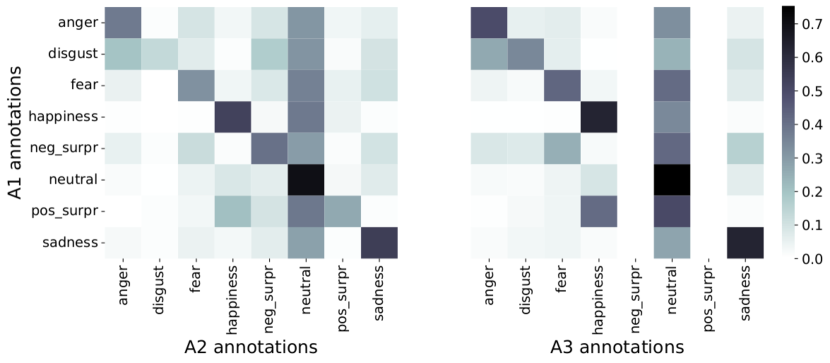
Figure 1: Confusion matrices comparing different annotators’ (A1, A2, A3) labels for the whole dataset. Note that for annotator 3, positive and negative surprise were not available.

Figure 1 shows confusion matrices comparing the annotations of annotator 1 with the annotations of annotators 2 and 3. The decision of whether a sentence is emotional or neutral is the most important source of disagreement in both annotator pairs. Furthermore, Figure 1 demonstrates that disagreement about the valence, i. e., pleasantness, of a sentence’s mood is rare. To give an example, in both depicted confusion matrices, sentences labeled with happiness by annotator 1 are rarely labeled with a negative emotion (anger, disgust, fear) by annotator 2 and 3, respectively.

3.2 Label Mapping

Motivated by low to moderate Krippendorff agreements (cf. Appendix B) and underrepresented classes in the discrete annotations (cf. Table 1), we project all emotion labels into the more generic, continuous valence/arousal space. Proposed by Russell (1980), the valence/arousal model characterizes affective states among two continuous dimensions where valence corresponds to pleasantness, while arousal is the intensity or degree of agitation. As depicted in Figure 1, the annotators often agree on the polarity of the emotion, i. e., whether it is to be understood as positive or negative in terms of valence. Hence, it can be argued that disagreement between annotators is not always as grave as suggested by low $\alpha$ values, which do not take proximity between different emotions into account. To give an example, disagreement on whether a sentence’s mood is happiness or neutral is certainly less severe than one annotator labeling the sentence sad, while the other opts for happy. Moreover, a projection into continuous space unifies the two different label spaces defined by the original and our additional annotations, respectively. To implement the desired mapping, we take up an idea proposed by Park et al. (2021), who map discrete emotion categories to valence and arousal values by looking up the label (e. g., anger) in the NRC-VAD dictionary Mohammad (2018) that assigns crowd-sourced valence and arousal values in the range $[0...1]$ to words. For instance, the label anger is mapped to a valence value of $.167$ and an arousal value of $.865$. The full mapping and further explanations can be found in Appendix C.

After label mapping, we create a gold standard for every story by fusing the thus obtained signals over the course of a story for valence and arousal, respectively. We apply the EWE Grimm and Kroschel (2005) method which is well-established for the problem of computing valence and arousal gold standards from continuous signals (e. g., Ringeval et al. (2019); Stappen et al. (2021); Christ et al. (2022b)). Figure 2 presents an example for this process, presenting both the discrete labels and the valence and arousal signals constructed from them for a specific story.

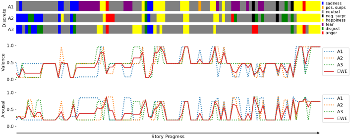
Figure 2: Exemplary mapping from the three annotators’ (A1, A2, A3) discrete annotations (top) to their respective valence (middle) and arousal (bottom) signals and the gold standard signals created via EWE (solid red lines). The annotations are taken from the story Ashputtel by the Grimm brothers, consisting of 102 sentences.

3.3 Split

We split the data on the level of stories. Three partitions for training, development, and test are created, with $118$, $25$, and $26$ stories, respectively. In doing so, we make sure to include comparable portions of stories and sentences by each author in all three partitions. A detailed breakdown is provided in Appendix D.

4 Experimental Setup

We fine-tune (cf. Section 4.1) the $304$M parameter large version of DeBERTaV3  He et al. (2023), additionally utilizing a weakly supervised learning approach (Section 4.2). Further details regarding the computational resources can be found in Appendix E.

4.1 Finetuning

Since the context of a sentence in a story is relevant to the mood it conveys, we seek to leverage multiple sentences at once in the fine-tuning process. Specifically, we create training examples as follows. We denote a story as a sequence of sentences $s_{1}\ldots s_{n}$. For a sentence $s_{i}$ and a context window size $\mathcal{C}$, we also consider the up to $\mathcal{C}$ sentences preceding ($s_{i-\mathcal{C}}\ldots s_{i-1}$) and the up to $\mathcal{C}$ sentences following ($s_{i+1}\ldots s_{i+\mathcal{C}}$) $s_{i}$. We construct an input string from the sentences $s_{i-\mathcal{C}}\ldots s_{i+\mathcal{C}}$ by concatenating them, separated via the special [SEP] token. The $i$-th [SEP] token in this sequence is intended to represent the $i$th sentence. We add a token-wise feed-forward layer on top of the last layer’s token representations. It projects each $1024$-dimensional embedding to $2$ dimensions and is followed by Sigmoid activation for both of them, corresponding to a prediction for valence and arousal, respectively. As the loss function, we sum up the Mean Squared Errors of valence and arousal predictions for each [SEP] token. We optimize $\mathcal{C}$, for $\mathcal{C}\in\{1,2,4,8\}$. If the length of an input exceeds the model’s capacity, we decrease $\mathcal{C}$ for this specific input. Figure 3 provides an example of an input sequence.

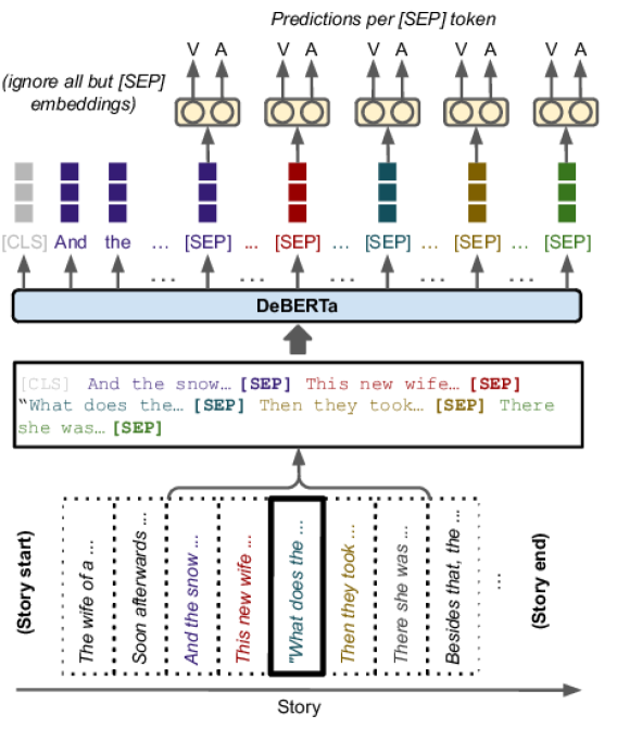
Figure 3: Example for the finetuning approach with context size $\mathcal{C}=2$. Valence (V) and arousal (A) predictions are obtained for all sentences at once.

We train the models for at most $10$ epochs but abort the training process early if no improvement on the development set is achieved for $2$ consecutive epochs. The evaluation metric is the mean of the Concordance Correlation Coefficient (CCC) Lawrence and Lin (1989) values achieved for arousal and valence, computed over the whole dataset, respectively. Equation 1 gives the formula for CCC between two signals $Y$ and $\hat{Y}$ of equal length.

$$\textit{CCC}(Y,\hat{Y})=\frac{2~{}\textit{Cov}(Y,\hat{Y})}{\textit{Var}(Y)+\textit{Var}(\hat{Y})+(\overline{Y}-\overline{\hat{Y}})^{2}}$$ (1)

CCC is a well-established correlation measure to assess agreement between (pseudo-)time continuous annotations and predictions, particularly common in Affective Computing Tasks, e. g., Ringeval et al. (2018); Schoneveld et al. (2021); Christ et al. (2023). It can be thought of as a bias-corrected modification of Pearson’s correlation. Different from Pearson’s correlation, it is sensitive to location and scale shifts, i. e., it measures not only correlation but also takes into account absolute errors. Same as for the Pearson correlation, the chance level is $0$, and two identical signals would have a CCC value of $1$. AdamW Loshchilov and Hutter (2019) is chosen as the optimization method. Following a preliminary hyperparameter search, the learning rate is set to $5\times 10^{-6}$. We do not optimise any hyperparameter besides the learning rate. Every experiment is repeated with five fixed seeds. In every experiment, we initialize the model with the checkpoint provided by the DeBERTaV3 authors.

4.2 Weakly Supervised Learning

The Alm dataset comprises $169$ stories by only three different authors, making our models prone to overfitting. Thus, we seek to augment our data set with in-domain texts written by other authors, thereby covering more topics and also spanning more cultures. We collect $45$ books containing in total $801$ different stories from Project Gutenberg, more specifically the Children’s Myths, Fairy Tales, etc. category. These stories comprise fairytales, myths, and other tales from different geographic regions, including Japan, Ireland, and India. This newly collected unlabeled data set, henceforth referred to as Gutenberg Corpus or Gb, amounts to $101529$ sentences. A more detailed description of Gb is given in Appendix F.

Figure 4 illustrates our overall finetuning approach. Given 1) a DeBERTa model finetuned on the labeled dataset (cf. 4.1), we 2) utilize its predictions on Gb as pseudo-labels, yielding a labeled dataset GbAlm. Subsequently, 3) another pretrained DeBERTa model is finetuned on GbAlm only. This training process is limited to $1$ epoch and employs a learning rate of $5\times 10^{-1}$. Lastly, 4) this model is further trained on Alm. Here, we utilize the same hyperparameters as for training $M$, but we find a smaller learning rate of $10^{-7}$ to be beneficial.

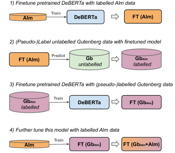
Figure 4: Illustration of our training steps and corpora. FT is short for finetuned.

5 Results

	FT Alm [CCC$\uparrow$]				FT GbAlm [CCC$\uparrow$]				FT GbAlm + Alm [CCC$\uparrow$]
	Valence		Arousal		Valence		Arousal		Valence		Arousal
$\mathcal{C}$	dev	test	dev	test	dev	test	dev	test	dev	test	dev	test
0	.6798	.6972	.5576	.5904	.6967	.7134	.5744	.6109	.7007	.7184	.5793	.6168
1	.7522	.7538	.6206	.6593	.7658	.7782	.6365	.6782	.7712	.7842	.6436	.6873
2	.7746	.7812	.6404	.6752	.7857	.7986	.6541	.6942	.7905	.8024	.6626	.7018
4	.7924	.7881	.6550	.6762	.7997	.8056	.6665	.6989	.8059	.8138	.6742	.7098
8	.7983	.7988	.6613	.6798	.8098	.8141	.6736	.7027	.8168	.8221	.6809	.7125

Table 2: Results for fine-tuning (FT) with different context sizes $\mathcal{C}$. See Figure 4 for an illustration of the three different corpora. The results are averaged over 5 fixed seeds. Standard deviations are negligible and thus omitted. Overall, the best results on the development set per prediction target and partition are boldfaced, and the best results for each context size are underlined.

Table 2 presents the results of our experiments with different $\mathcal{C}$ values. We report the mean CCC results when tuning a) only on Alm (FT Alm, step 1 in Figure 4), b) only on GbAlm (FT GbAlm, step 3 in Figure 4) and c) additionally on Alm (FT GbAlm + Alm, step 4 in Figure 4). There is a clear trend for both arousal and valence to increase with larger $\mathcal{C}$s. The models trained with a context size of $8$ account for the best valence and arousal results in every set of experiments, e. g., CCC values of $.8168$ and $.6809$ for arousal and valence, respectively, on the development set when trained on both corpora. These are also the best results encountered overall. In contrast, the models with $\mathcal{C}=0$ always perform worst, yielding e. g., only CCC values of $.6798$ (valence) and $.5576$ (arousal) on the development set in the Alm-only configuration. This supports the assumption that the context of a sentence is oftentimes key to correctly assessing its mood. The gap between valence and arousal CCC values is in line with previous studies showing that text-based classifiers are typically better suited for valence prediction than for arousal prediction Kossaifi et al. (2019); Wagner et al. (2023). Further, our results demonstrate the benefits of the weakly supervised approach. Training on GbAlm always improves upon training on Alm only, especially for smaller context sizes $\mathcal{C}$. To give an example, both the valence and arousal CCC values on the development set increase by more than $1.5$ for $\mathcal{C}=0$ on the development set. Further tuning on Alm afterward leads to additional performance gains for both prediction targets and all context sizes. However, the increase never exceeds $1$ percentage point in comparison to training on GbAlm.

5.1 Author-Wise Results

[CCC$\uparrow$]	Auth
	Grimm		HCA		Potter
Finetuning (FT)	Valence	Arousal	Valence	Arousal	Valence	Arousal
Alm	.7943	.6804	.7942	.6881	.7606	.6442
GbAlm	.8131	.7104	.8247	.7253	.7672	.6761
Alm$\setminus\{$Auth$\}$	.7597	.6505	.7633	.6563	.7304	.5886
GbAlm$\setminus\{$Auth$\}$	.7799	.6734	.7837	.6774	.7386	.6344

Table 3: Author-wise experiment results on the respective test sets. The results are averaged and standard deviations (all $<.01$) are omitted. Cf. Figure 4 for illustration of the methods.

Since Alm comprises stories of three different authors, we investigate the relevance of an author’s individual style for learning to predict their stories. For each author (Auth), we create a dataset Alm$\setminus\{\textsc{Auth}\}$ by removing Auth’s stories from the training and development partitions and keeping only Auth’s stories as test data. We then repeat steps 1-3 in  Figure 4, using Alm$\setminus\{\textsc{Auth}\}$ instead of the full Alm dataset. Only the best configuration, i. e., $\mathcal{C}=8$ is considered here. The results of these experiments, alongside the corresponding author-wise results, when employing the full Alm dataset, are given in Table 3. Performance, in general, differs by author, e. g., both valence and arousal CCC for Potter are lower than for the other two authors when training on the full Alm dataset. Furthermore, test set performance for every author drops when removing the author from the training and development data. The clearest example is Potter’s arousal CCC value of $.5886$ when training on Alm$\setminus\{\textit{Potter}\}$ compared to $.6442$ when training on the full Alm data. The weakly supervised learning step, implying exposure to a wider range of styles, proves to be beneficial for every author, regardless of the dataset. Nevertheless, for every author Auth the performance of the weakly supervised approach on Alm$\setminus\{\textsc{Auth}\}$ never reaches the performance for fine-tuning on Alm alone. In conclusion, it is crucial to include targeted authors in training data in order to capture their individual styles.

5.2 Further Statistics

In the remainder of the paper, we limit our analysis to the best-performing seed for $\mathcal{C}=8$ and the full training pipeline (cf. Figure 4).

The CCC values given in Table 2 are calculated over the entire dataset, i. e., a concatenation of all stories per partition. Table 4, in contrast, lists story-wise CCC results for the predictions of our best model.

Partition	Valence [CCC$\uparrow$]	Arousal [CCC$\uparrow$]
Dev	.7729 ($\pm$.1207)	.6892 ($\pm$.0812)
Test	.7685 ($\pm$.0946)	.6352 ($\pm$.1679)

Table 4: Story-wise CCC results over all stories in the development and test set as predicted by the best model.

It shows that results are highly story-dependent. To give an example, the arousal CCC values for the test partition display a standard deviation of $.1679$ over the $25$ stories in this partition.

We find that the model’s performance for arousal and valence per story correlates: we obtain a Pearson’s correlation of $.3499$ (statistically significant with $p<.02$) between our best model’s valence CCC values per story and the respective CCC arousal values. Hence, there exist stories whose emotional trajectories are difficult (or easy) to predict for the model in general, regardless of the two different emotional dimensions.

This can partly be explained by the correlation between model performance and human agreement per story. There is a Pearson’s correlation of $.3659$ between all story-wise human CCC agreements and the CCC values achieved by the best model on the corresponding stories. Analogously, for arousal, this correlation is $.4095$. Both correlations are statistically significant with $p<.02$. It can be concluded that the model particularly struggles to learn stories that also pose a challenge to humans.

Another analysis reveals that the model’s performance also tends to vary for different parts of the same story. We divide every story into 5 parts of equal size. This way, we evaluate the performance of our best models on 5 different subsets of the data corresponding to positions in the story. Roughly, the first part can be expected to correspond to the beginning of the story, while the last part comprises its end. Table 6 displays the results of this evaluation. Both valence and arousal results are, on average, better at the very beginning ($.8260$ valence, $.7304$ arousal CCC) and the very end ($.8576$ valence, $.7306$ arousal CCC) of the stories than during their middle parts. We hypothesize that this is due to many stories’ beginnings and endings being drawn from a limited set of archetypical situations. Hence, the model may easily learn the emotional connotations of such common events from the large corpus. To give a few examples, fairytales in particular often start, e. g., with the death or absence of a parent, the hero leaving home, an act of villainy against the hero, or a combination thereof. Endings often involve reunion, marriage, and the villain receiving punishment Propp (1968).

As a measure of model performance on the sentence level, we compute the best model’s absolute prediction errors on the development and test set. Table 5 presents the results.

	mean	std	median	perc. $90$	perc. $95$
Valence	.1001	.0971	.0721	.2302	.2940
Arousal	.1205	.1144	.0838	.2878	.3626

Table 5: Absolute error statistics for the development and test data predictions (combined) of the best model.

It is evident from the median values that more than half of arousal and valence predictions miss the gold standard by less than $.1$. From the percentiles, it can be concluded that errors larger than $.3$ occur in less than $5\,\%$ of sentences for valence and in less than $10\,\%$ of sentences for arousal.

[CCC$\uparrow$]	Story Part
	$1$/$5$	$2$/$5$	$3$/$5$	$4$/$5$	$5$/$5$
Valence	.8260	.8044	.8091	.7785	.8576
Arousal	.7304	.6543	.6814	.6618	.7306

Table 6: Mean CCC values across 5 seeds for the best configuration on different story parts. We omit the low standard deviations(all $<1$), omitted. Results were computed over the unification of test and dev.

5.3 Qualitative Analysis

To gain qualitative insights into the model’s limitations, we manually analyze around $200$ text spans for which high absolute errors in terms of valence or arousal prediction are observed. First, we find that the model seems to learn emotional connotations of events, but is prone to ignore the roles of the protagonists involved in them. Table 7 provides an example of this phenomenon. In this text passage, a typically positive event, namely being granted a wish, is salient. The model assigns relatively high valence values. However, the actual mood in these sentences is rather negative, as they describe the implicitly jealous reaction of a negative character to this situation.

Story: 87_the_poor_man_and_the_rich_man (Grimms)
Context: A poor man receives a new house as a reward from God. His
neighbor (rich man) sees the new house and gets jealous.
Sentence	V pred	V GS
The sun was high when the rich man got up and leaned out of his window and saw, on the opposite side of the way, a new clean-looking house with red tiles and bright windows where the old hut used to be.	.8044	.4690
He was very much astonished, and called his wife and said to her, "Tell me, what can have happened?	.5657	.2220
Last night there was a miserable little hut standing there, and to-day there is a beautiful new house.	.7744	.2220

Table 7: Passage from 87_the_poor_… (Grimms) with valence (V) predictions (pred) and gold standard (GS).

Probably closely related to these observations, we figure that our model sometimes struggles to accurately assess situations, because it disregards the general sentiment of the respective story. To give an example, Table 8 lists a passage from Andersen’s story grandmot. This story displays a rather positive sentiment overall, as it is presented as a loving memory of a deceased grandmother. For the passages describing her peaceful death, our model underestimates the valence gold standard by a large margin, probably due to the typically sad topic of death.

Story: grandmot (Andersen)
Context: The story is about a beloved grandmother and her peaceful death
Sentence	V pred	V GS
She smiled once more, and then people said she was dead.	.3053	.6470
She was laid in a black coffin, looking mild and beautiful […] though her eyes were closed; but every wrinkle had vanished, her hair looked white and silvery, and around her mouth lingered a sweet smile.	.2902	.7910
We did not feel at all afraid to look at the corpse of her who had been such a dear, good grandmother.	.3197	.4700

Table 8: Passage from grandmot (Andersen) with valence (V) predictions (pred) and gold standard (GS).

Stories within stories pose another facet the model faces difficulties with. Frequently, protagonists tell stories or recall memories. Narrated stories or memories typically contain emotionally significant events, but they are not directly experienced and thus are not always heavily influencing the mood of the actual story. Table 9 presents an example, where a cat tells another one about a fearful incident. The corresponding gold standard arousal values are moderate, arguably as the incident is over and has not harmed the protagonist. The model nevertheless predicts high arousal.

Story: the_roly-poly_pudding (Potter)
Context: A cat tells another cat (Ribby) how he had encountered a rat.
Sentence	A pred	A GS
I caught seven young ones [rats] […], and we had them for dinner last Saturday.	.6566	.1840
And once I saw the old father rat –an enormous old rat – Cousin Ribby.	.5070	.3940
I was just going to jump upon him, when he showed his yellow teeth at me and whisked down the hole.	.7283	.1840

Table 9: Passage from the_roly_poly… (Potter) with arousal (A) predictions (pred) and gold standard (GS).

To summarise, the model tends to miss out on a holistic understanding of stories such as the roles of different protagonists, nested stories, and a story’s overall tone. This can partially be attributed to inputs not consisting of complete stories, cf. Section 4.1. Further examples for all aspects discussed above can be found in Appendix G.

6 Discussion

We demonstrate the efficacy of our approach to model emotional trajectories via LLMs, achieving CCC values of $.8221$ and $.6809$ for valence and arousal on the test set, respectively. We find that considering a sentence’s context is crucial for predicting its emotionality. Furthermore, our analysis reveals the author-dependence of these results, which, in addition, vary from story to story. Even within a story, certain parts (namely, beginning and ending) are often easier to predict than others. Further analysis of our models’ predictions uncovers additional challenges, such as assigning the correct role to protagonists and understanding the overall tone of a story. All these aspects combined shed light on the complexity of the task at hand. Keeping this in mind, our methodology can be understood as a first benchmark for predicting emotional trajectories in a supervised manner.

7 Conclusion

We proposed a valence/arousal-based gold standard for the Alm dataset Alm (2008). Moreover, we provide first results for the prediction of these signals via finetuning DeBERTa combined with a weakly supervised learning step. We obtain promising results, but, at the same time, demonstrate the limits of this methodology in our analysis. Future work may include attempts at a more holistic story understanding, involving e. g., the roles of protagonists. Besides, our analysis of the results by author suggests that personalization methods (e. g., Kathan et al. (2022)) may improve the results. Further, the potential of even larger LLMs such as LLaMA Touvron et al. (2023) or (Chat-)GPT Achiam et al. (2023) remains to be explored for this task. Such models may even assist in refining the rather simplistic mapping method we utilized for the creation of the gold standard, as they have been shown to come with inherent emotional understanding capabilities Broekens et al. (2023); Tak and Gratch (2023). Code, data, and model weights are released to the public.

8 Limitations

Our work comes with several constraints. The simple mapping from discrete emotions into the dimensional valence/arousal space (cf. Table 12) may be too coarse to capture some texts’ emotional connotations. When analyzing the best model’s predictions, we encounter texts where such shortcomings of our label mapping approach (cf. Table 12) surface. For instance, all instances of disgust are mapped to high arousal, leaving no room for less frequent low-arousal variants of disgust as can be found in passages like the one given in Table 10. Here, the sentences’ mood was predominantly labeled as disgust and thus set to high gold standard arousal values. The considerably lower arousal predictions by our model, however, are arguably more appropriate than the gold standard here, as the described situation is rather characterized by distanced arrogance than by actual disgust.

Story: good_for (Andersen)
Context: An arrogant man sees a drunk poor woman from his window.
Sentence	A pred	A GS
“Oh, it is the laundress,” said he; “she has had a little drop too much.	.3335	.8050
She is good for nothing.	.5281	.6340
It is a sad thing for her pretty little son.	.3242	.6700

Table 10: Passage from good_for (Andersen) with arousal predictions (pred) and gold standard (GS).

Besides, our approach to weakly supervised learning is obviously limited to high-resource languages. Story is a broad term applicable to all texts in both Alm and the crawled Gb data. The included stories could be distinguished in a more fine-grained manner, e. g., the data contains fairytales, myths, fables, and other types of stories. Such distinctions may have methodologically relevant implications we do not consider in our experiments. We also show that emotional arcs are highly author-dependent (cf. Section 5.2), implying that future datasets should seek to comprise a wider range of authors and writing styles. In particular, our results may not generalize well to authors of backgrounds that are not represented in the data used. Lastly, we analyse our method’s limitations in Section 5.3, without claim of completeness.

Appendix A Annotation Details

Our additional annotations (cf. Section 3.1) are carried out by a 24-year-old male PhD student with a solid background in Affective Computing concepts, in particular, different emotion models. Hence, A3 is the same person for all stories, while this is not the case for A1 and A2 (cf. Alm and Sproat (2005); Alm (2008)). Figure 5 shows a screenshot of the annotation tool.

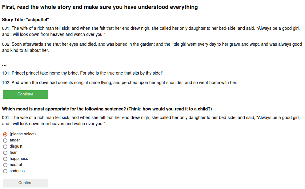
Figure 5: Screenshot of the annotation tool. First, the whole story must be read. Upon confirmation (“Continue”), annotation of the individual sentences follows.

Appendix B Agreement Statistics

Krippendorff’s alpha ($\alpha$) for all three annotators is $.385$, when calculated based on single sentences and ignoring the different label schemes. This is possible, as annotator 3’s label scheme is a subset of the labels available to annotators 1 and 2. The mean $\alpha$ per story is $\mu_{\alpha}=.341$, with a standard deviation of $\sigma_{\alpha}=.126$, indicating that the level of agreement is highly dependent on the story. We remove stories whose $\alpha$ is smaller than $\mu_{\alpha}-2\sigma_{\alpha}$. A detailed listing of $\alpha$ values for the remaining data on both the sentence and the story level is provided in Table 11.

Annotators	Level	Overall	Grimms	HCA	Potter
A1,A2	sent.	.356	.272	.411	.333
	story	.297 ($\pm$.174)	.245 ($\pm$.196)	.350 ($\pm$.149)	.307 ($\pm$.073)
A1,A3	sent.	.420	.370	.447	.433
	story	.376 ($\pm$.184)	.346 ($\pm$.212)	.395 ($\pm$.158)	.428 ($\pm$.126)
A2,A3	sent.	.383	.331	.408	.391
	story	.338 ($\pm$.176)	.296 ($\pm$.172)	.376 ($\pm$.178)	.3614 ($\pm$.139)
A1,A2,A3	sent.	.387	.325	.422	.390
	story	.343 ($\pm$.126)	.301 ($\pm$.133)	.380 ($\pm$.118)	.370 ($\pm$.062)

Table 11: $\alpha$ values for all possible combinations of annotators. The values are given for the whole dataset (Overall) and the individual authors (Grimms, HCA, Potter). The sent. rows report the alphas on the basis of sentence annotations, in story rows, the means, as well as standard deviations of alpha values per story, can be found.

Table 11 illustrates that agreement is also author-dependent, e. g., for all combinations of annotators, the sentence-wise agreement for the Grimm brothers is lower than for both other authors.

Appendix C Label Mapping Details

Table 12 lists the mapping for all discrete emotion labels as obtained from the NRC-VAD dictionary Mohammad (2018). However, the dictionary does not contain entries for positive surprise and negative surprise. For positive surprise, we take the valence and arousal values of surprise (both $.875$). The valence value for negative surprise is set to the mean valence value of the negative emotions anger, disgust, and fear ($.097$), while the arousal value is the same as for positive surprise ($.875$).

Label	Valence	Arousal
Anger	.167	.865
Disgust	.052	.775
Fear	.073	.840
Happiness	.960	.732
Negative Surprise	.097	.875
Neutral	.469	.184
Positive Surprise	.875	.875
Sadness	.052	.288

Table 12: Mapping from discrete labels to continuous valence and arousal values.

There are a few similar attempts to mapping discrete to continuous emotion models, but no agreed-upon gold standard method to do so. Our decision for this particular method is motivated by three criteria: 1) the method should yield a numeric value (in contrast to approaches like Amiriparian et al. (2024); Gerczuk et al. (2021) that utilize categories such as “low valence” etc.) 2) the values should, of course, match our expectations based on Russel’s circumplex model Russell (1980) regarding the position of the discrete emotions in the V/A space, and 3) the method must be able to account for all labels in the dataset. We could, e.g., not utilize the V/A mappings for discrete emotions collected in Hoffmann et al. (2012), as they do not obtain values for surprise, disgust, and neutral. Admittedly, the method we selected has this problem for negative surprise as well, but we found a relatively straightforward way to make up for this shortcoming.

We validate the mapping approach by obtaining additional valence/arousal labels from the same annotator for $3$ randomly selected stories. Table 13 reports the Pearson correlation between these direct valence/arousal annotations and those obtained by the proposed mapping.

Story (author)	$\rho$ Valence	$\rho$ Arousal
emperor (Andersen)	.7943	.6151
hansel_and_gretel (Grimms)	.8498	.5765
the_tale_of_jemima… (Potter)	.7504	.6088

Table 13: Mapping approach validation on three stories. Reported are Pearson’s correlations between direct V/A annotations and pseudo-V/A annotations as computed by the mapping from discrete labels.

The correlations illustrate again that the difficulty of the problem varies for different stories. Moreover, the correlations for valence are higher than those for arousal, indicating that the method may capture valence better than arousal. This observation may also contribute to explaining why the automatic prediction of arousal proves to be more difficult than the prediction of valence.

Appendix D Split Statistics

Table 14 displays detailed statistics for the split into training, development, and test sets.

	Overall	Grimm	HCA	Potter
train
stories	118	54 (45.76 %)	51 (43.22 %)	13 (11.02 %)
sentences	10,121	3,621 (35.78 %)	5,246 (51.38 %)	1,254 (12.39 %)
development
stories	25	9 (36.00 %)	13 (52.00 %)	3 (12.00 %)
sentences	2,384	604 (25.34 %)	1,494 (58.47 %)	386 (16.19 %)
test
stories	26	14 (53.85 %)	9 (34.62 %)	3 (11.54 %)
sentences	2,379	1 011 (42.50 %)	1 072 (45.06 %)	296 (12.44 %)

Table 14: Dataset split statistics for every partition and author. For each author, the absolute number of stories as well as sentences in each partition is given. The percentage values denote the share of the author’s stories/sentences in the stories/sentences of the respective partition.

Figure 6 shows that the continuous label distributions are fairly similar in the different partitions.

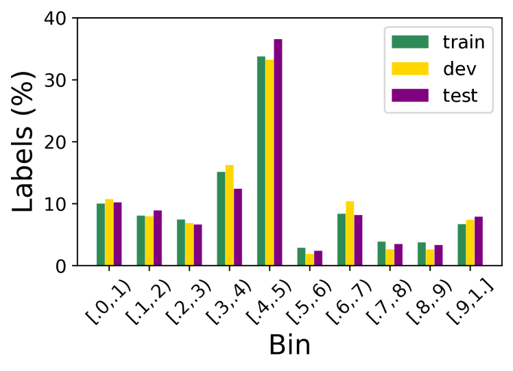
(a) Valence Values

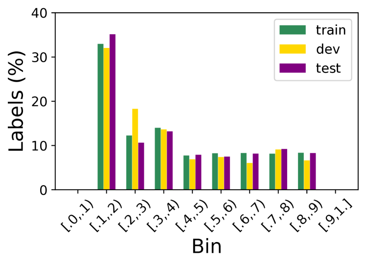
(b) Arousal Values

Figure 6: Distributions of binned valence and arousal values in the created training, development (dev), and test partitions.

Appendix E Further Experiment Details

All experiments were carried out on an NVIDIA RTX3090 GPU and took about $200$ GPU hours in total. For illustration, we calculate the rough number of training/prediction steps for one experiment, i. e., one configuration (e. g., $C=4$) and one seed. The Alm dataset comprises about $15$k data points (about $10$k of which are used for training), the Gutenberg dataset contains about $100$k sentences. Assuming that steps 1) and 4) in Figure 4 run for 5 epochs each and step 3) takes one epoch, all of them using a batch size of 4, we end up with $(5*(100$k$+10$k$)+110$k$)/4=165$k training steps. Multiplying this with $5$ seeds and $5$ $C$-configurations, results in about $4$M training steps overall, notwithstanding some preliminary hyperparameter optimization and the additional author-independent experiments. These rather large resource requirements also motivate our choice for the relatively small $304$M parameter DeBERTa model.

Appendix F Gutenberg Corpus

In Table 21, all books used for creating the Gb are listed. We make sure not to include tales written by the three authors in the labeled dataset. We do not carry out any further filtering or manual screening steps. Basic preprocessing steps such as the removal of footnotes and images are conducted before we split the stories into sentences utilizing the PySBD Sadvilkar and Neumann (2020) library.

Appendix G Further Qualitative Analysis

In this section, we provide further examples of passages for which the model’s predictions result in large errors, thus extending Section 5.3.

Table 15 displays a text passage revolving around the theme of marriage. The model predicts high valence values, arguably due to this oftentimes positive topic. However, in this particular context, the planned marriage is viewed as negative by the protagonist.

Story: li_tiny (Andersen)
Context: Protagonist (Tiny) is about to get married against her will.
Sentence	V pred	V GS
“You are going to be married, Tiny,” said the field-mouse.	.8392	.052
"My neighbor has asked for you.	.4902	.469
What good fortune for a poor child like you.	.7692	.469

Table 15: Passage from li_tiny (Andersen) with valence predictions (pred) and gold standard (GS).

In Table 16, an example is provided in which the model assesses a situation as positive, in which a person has gained a great amount of power. The gold standard, in contrast, assigns low valence values to this passage, as the protagonist exhibits greed and megalomania, aspects seemingly ignored by the model.

Story: the_fisherman_and_his_wife (Grimms)
Context: The protagonist’s wife (Ilsabill) has acquired an absurd amount of power.
Sentence	V pred	V GS
Then the fisherman went home, and found Ilsabill sitting on a throne that was two miles high.	.5495	.200
And she had three great crowns on her head, and around her stood all the pomp and power of the Church.	.6597	.357
And on each side of her were two rows of burning lights, of all sizes, the greatest as large as the highest and biggest tower in the world, and the least no larger than a small rushlight.	.6668	.357

Table 16: Passage from the_fisherman_and_his_wife (Grimms) with valence predictions (pred) and gold standard (GS).

The phenomenon of our model missing out on the overall tone of stories is further exemplified by the text in Table 17. Here, the protagonists are pigs behaving like and interacting with humans, which gives the entire story a funny mood. In this context, a typically rather exciting situation (being interrogated by the police) is not assigned a high arousal value by the gold standard – different from the model.

Story: the_tale_of_pigling_bland (Potter)
Context: Pigs are interrogated by a policeman.
Sentence	A pred	A GS
What’s that, young Sirs?	.5057	.184
Stole a pig?	.5014	.184
Where are your licenses? said the policeman.	.6877	.184

Table 17: Passage from the_tale_of… (Potter) with arousal predictions (pred) and gold standard (GS).

Another example from an overall funny story is given in Table 18. The protagonists encounter several robbers, but the situation is labeled with a neutral valence value in the gold standard. The model assigns low valence values, missing out on the funny tone of the entire story.

Story: frederick_and_catherine (Grimms)
Context: Protagonists (Frederick and Catherine) encounter robbers.
Sentence	V pred	V GS
Scarcely were they up, than who should come by but the very rogues they were looking for.	.2310	.469
They were in truth great rascals, and belonged to that class of people who find things before they are lost; they were tired; so they sat down and made a fire under the very tree where Frederick and Catherine were.	.2891	.469

Table 18: Passage from frederick_and_catherine (Grimms) with valence predictions (pred) and gold standard (GS).

Moreover, we provide further examples of the model struggling with stories within stories. In the passage given in Table 19, the model overestimates the arousal value, as the story told about a great fire is arguably very exciting.

Story: a_story (Andersen)
Context: A man recounts a memory where he witnessed a fire.
Sentence	A pred	A GS
All burnt down- a great heat rose, such as sometimes overcomes me.	.6779	.460
I myself helped to rescue cattle and things, nothing alive burnt, except a flight of pigeons, which flew into the fire, and the yard dog, of which I had not thought; one could hear him howl out of the fire, and this howling I still hear when I wish to sleep; and when I have fallen asleep, the great rough dog comes and places himself upon me, and howls, presses, and tortures me.	.7914	.288

Table 19: Passage from a_story (Andersen) with arousal predictions (pred) and gold standard (GS).

The example presented in Table 20 demonstrates a passage where valence is overestimated by the model. Here, happy memories are recalled in a sad context, giving the text a sad mood that is not properly assessed by the model.

Story: old_bach (Andersen)
Context: a sad old bachelor recalls his youth.
Sentence	V pred	V GS
How much came back to his remembrance as he looked through the tears once more on his native town!	.8102	.469
The old house was still standing as in olden times, but the garden had been greatly altered; a pathway led through a portion of the ground, and outside the garden, and beyond the path, stood the old apple-tree, which he had not broken down, although he talked of doing so in his trouble.	.7996	.469
The sun still threw its rays upon the tree, and the refreshing dew fell upon it as of old; and it was so overloaded with fruit that the branches bent towards the earth with the weight.	.9574	.634

Table 20: Passage from old_bach (Andersen) with valence predictions (pred) and gold standard (GS).

Gutenberg ID	Book Title
22656	Red Cap Tales, Stolen from the Treasure Chest of the Wizard of the North
19713	The Laughing Prince: Jugoslav Folk and Fairy Tales
4357	American Fairy Tales
19207	The Firelight Fairy Book
17034	English Fairy Tales
24714	Fairy Tales from Brazil: How and Why Tales from Brazilian Folk-Lore
20748	Favorite Fairy Tales
20366	Wonderwings and other Fairy Stories
7439	English Fairy Tales
24593	The Oriental Story Book: A Collection of Tales
22420	The Book of Nature Myths
19734	The Fairy Book
8599	Fairy Tales from the Arabian Nights
9368	Welsh Fairy Tales
16537	Myths That Every Child Should Know
24473	The Cat and the Mouse: A Book of Persian Fairy Tales
22168	The golden spears, and other fairy tales
25502	Hero-Myths & Legends of the British Race
22175	Stories from the Ballads, Told to the Children
24737	The Children of Odin: The Book of Northern Myths
22693	A Book of Myths
677	The Heroes; Or, Greek Fairy Tales for My Children
23462	More Russian Picture Tales
15145	My Book of Favourite Fairy Tales
4018	Japanese Fairy Tales
11319	The Fairy Godmothers and Other Tales
15164	Folk Tales Every Child Should Know
7871	Dutch Fairy Tales for Young Folks
7488	Celtic Tales, Told to the Children
14916	Fairy Tales Every Child Should Know
20552	Roumanian Fairy Tales
2892	Irish Fairy Tales
7885	Celtic Fairy Tales
22096	Stories the Iroquois Tell Their Children
25555	Fairy Tales of the Slav Peasants and Herdsmen
14421	Wilson’s Tales of the Borders and of Scotland, Volume 24
7128	Indian Fairy Tales
6622	Legends That Every Child Should Know; a Selection of the Great Legends of All…
8675	Welsh Fairy-Tales and Other Stories
22373	Russian Fairy Tales: A Choice Collection of Muscovite Folk-lore
22886	Cinderella in the South: Twenty-Five South African Tales
22248	The Indian Fairy Book: From the Original Legends
24811	Viking Tales
18674	A Chinese Wonder Book
22396	King Arthur’s Knights

Table 21: List of books in the Gutenberg corpus.

References

- Achiam et al. (2023) Josh Achiam, Steven Adler, Sandhini Agarwal, Lama Ahmad, Ilge Akkaya, Florencia Leoni Aleman, Diogo Almeida, Janko Altenschmidt, Sam Altman, Shyamal Anadkat, et al. 2023. Gpt-4 technical report. arXiv preprint arXiv:2303.08774.
- Agrawal and An (2012) Ameeta Agrawal and Aijun An. 2012. Unsupervised emotion detection from text using semantic and syntactic relations. In 2012 IEEE/WIC/ACM International Conferences on Web Intelligence and Intelligent Agent Technology, volume 1, pages 346–353. IEEE.
- Alm et al. (2005) Cecilia Ovesdotter Alm, Dan Roth, and Richard Sproat. 2005. Emotions from text: Machine learning for text-based emotion prediction. In Proceedings of Human Language Technology Conference and Conference on Empirical Methods in Natural Language Processing, pages 579–586, Vancouver, British Columbia, Canada. Association for Computational Linguistics.
- Alm and Sproat (2005) Cecilia Ovesdotter Alm and Richard Sproat. 2005. Emotional sequencing and development in fairy tales. In International Conference on Affective Computing and Intelligent Interaction, pages 668–674. Springer.
- Alm (2008) Ebba Cecilia Ovesdotter Alm. 2008. Affect in Text and Speech. University of Illinois at Urbana-Champaign.
- Amiriparian et al. (2024) Shahin Amiriparian, Filip Packan, Maurice Gerczuk, and Björn W. Schuller. 2024. ExHuBERT: Enhancing HuBERT Through Block Extension and Fine-Tuning on 37 Emotion Datasets. In Proc. INTERSPEECH, Kos Island, Greece. ISCA. To appear.
- Amiriparian et al. (2023) Shahin Amiriparian, Bjorn W Schuller, Nabiha Asghar, Heiga Zen, and Felix Burkhardt. 2023. Guest editorial: Special issue on affective speech and language synthesis, generation, and conversion. IEEE Transactions on Affective Computing, 14(01):3–5.
- Batbaatar et al. (2019) Erdenebileg Batbaatar, Meijing Li, and Keun Ho Ryu. 2019. Semantic-emotion neural network for emotion recognition from text. IEEE Access, 7:111866–111878.
- Broekens et al. (2023) Joost Broekens, Bernhard Hilpert, Suzan Verberne, Kim Baraka, Patrick Gebhard, and Aske Plaat. 2023. Fine-grained affective processing capabilities emerging from large language models. In 2023 11th International Conference on Affective Computing and Intelligent Interaction (ACII), pages 1–8. IEEE.
- Burke (2015) Michael Burke. 2015. The neuroaesthetics of prose fiction: Pitfalls, parameters and prospects. Frontiers in Human Neuroscience, 9:442.
- Christ et al. (2023) Lukas Christ, Shahin Amiriparian, Alice Baird, Alexander Kathan, Niklas Müller, Steffen Klug, Chris Gagne, Panagiotis Tzirakis, Lukas Stappen, Eva-Maria Meßner, et al. 2023. The muse 2023 multimodal sentiment analysis challenge: Mimicked emotions, cross-cultural humour, and personalisation. In Proc. MuSe, pages 1–10.
- Christ et al. (2022a) Lukas Christ, Shahin Amiriparian, Alice Baird, Panagiotis Tzirakis, Alexander Kathan, Niklas Müller, Lukas Stappen, Eva-Maria Meßner, Andreas König, Alan Cowen, Erik Cambria, and Björn W. Schuller. 2022a. The muse 2022 multimodal sentiment analysis challenge: Humor, emotional reactions, and stress. In MuSe’22: Proceedings of the 3rd Multimodal Sentiment Analysis Workshop and Challenge, pages 5–14, Lisbon, Portugal. Association for Computing Machinery. Co-located with ACM Multimedia 2022.
- Christ et al. (2022b) Lukas Christ, Shahin Amiriparian, Alexander Kathan, Niklas Müller, Andreas König, and Björn W Schuller. 2022b. Towards multimodal prediction of spontaneous humour: A novel dataset and first results. arXiv preprint arXiv:2209.14272.
- Devlin et al. (2019) Jacob Devlin, Ming-Wei Chang, Kenton Lee, and Kristina Toutanova. 2019. BERT: Pre-training of deep bidirectional transformers for language understanding. pages 4171–4186.
- Eisenreich et al. (2014) Christian Eisenreich, Jana Ott, Tonio Süßdorf, Christian Willms, and Thierry Declerck. 2014. From tale to speech: Ontology-based emotion and dialogue annotation of fairy tales with a tts output. In ISWC-PD’14: Proceedings of the 2014 International Conference on Posters & Demonstrations Track - Volume 1272.
- Gerczuk et al. (2021) Maurice Gerczuk, Shahin Amiriparian, Sandra Ottl, and Björn W Schuller. 2021. Emonet: A transfer learning framework for multi-corpus speech emotion recognition. IEEE Transactions on Affective Computing, 14(2):1472–1487.
- Gottschall (2012) Jonathan Gottschall. 2012. The Storytelling Animal: How Stories Make Us Human. Houghton Mifflin Harcourt.
- Grimm and Kroschel (2005) Michael Grimm and Kristian Kroschel. 2005. Evaluation of natural emotions using self assessment manikins. In IEEE Workshop on Automatic Speech Recognition and Understanding, 2005., pages 381–385. IEEE.
- He et al. (2023) Pengcheng He, Jianfeng Gao, and Weizhu Chen. 2023. DeBERTav3: Improving deBERTa using ELECTRA-style pre-training with gradient-disentangled embedding sharing. In The Eleventh International Conference on Learning Representations.
- Hoffmann et al. (2012) Holger Hoffmann, Andreas Scheck, Timo Schuster, Steffen Walter, Kerstin Limbrecht, Harald C Traue, and Henrik Kessler. 2012. Mapping discrete emotions into the dimensional space: An empirical approach. In 2012 IEEE International Conference on Systems, Man, and Cybernetics (SMC), pages 3316–3320. IEEE.
- Hogan (2011) Patrick Colm Hogan. 2011. Affective Narratology: The Emotional Structure of Stories. U of Nebraska Press.
- Kathan et al. (2022) Alexander Kathan, Shahin Amiriparian, Lukas Christ, Andreas Triantafyllopoulos, Niklas Müller, Andreas König, and Björn W Schuller. 2022. A personalised approach to audiovisual humour recognition and its individual-level fairness. In Proceedings of the 3rd International on Multimodal Sentiment Analysis Workshop and Challenge, pages 29–36.
- Kim and Klinger (2018a) Evgeny Kim and Roman Klinger. 2018a. A survey on sentiment and emotion analysis for computational literary studies. arXiv preprint arXiv:1808.03137.
- Kim and Klinger (2018b) Evgeny Kim and Roman Klinger. 2018b. Who feels what and why? annotation of a literature corpus with semantic roles of emotions. In Proceedings of the 27th International Conference on Computational Linguistics, pages 1345–1359, Santa Fe, New Mexico, USA. Association for Computational Linguistics.
- Kim et al. (2017) Evgeny Kim, Sebastian Padó, and Roman Klinger. 2017. Prototypical emotion developments in literary genres. In Proceedings of the Joint SIGHUM Workshop on Computational Linguistics for Cultural Heritage, Social Sciences, Humanities and Literature, pages 17–26.
- Kossaifi et al. (2019) Jean Kossaifi, Robert Walecki, Yannis Panagakis, Jie Shen, Maximilian Schmitt, Fabien Ringeval, Jing Han, Vedhas Pandit, Antoine Toisoul, Björn Schuller, et al. 2019. Sewa db: A rich database for audio-visual emotion and sentiment research in the wild. IEEE transactions on pattern analysis and machine intelligence, 43(3):1022–1040.
- Lawrence and Lin (1989) I Lawrence and Kuei Lin. 1989. A concordance correlation coefficient to evaluate reproducibility. Biometrics, pages 255–268.
- Liu et al. (2019) Chen Liu, Muhammad Osama, and Anderson De Andrade. 2019. DENS: A dataset for multi-class emotion analysis. pages 6293–6298.
- Loshchilov and Hutter (2019) Ilya Loshchilov and Frank Hutter. 2019. Decoupled weight decay regularization. In International Conference on Learning Representations.
- Lugrin et al. (2010) Jean-Luc Lugrin, Marc Cavazza, David Pizzi, Thurid Vogt, and Elisabeth André. 2010. Exploring the usability of immersive interactive storytelling. In Proceedings of the 17th ACM symposium on virtual reality software and technology, pages 103–110.
- Mani (2014) Inderjeet Mani. 2014. Computational narratology. Handbook of narratology, pages 84–92.
- Mohammad (2018) Saif Mohammad. 2018. Obtaining reliable human ratings of valence, arousal, and dominance for 20,000 english words. In Proceedings of the 56th annual meeting of the association for computational linguistics (volume 1: Long papers), pages 174–184.
- Moreira et al. (2023) Pascale Moreira, Yuri Bizzoni, Kristoffer Nielbo, Ida Marie Lassen, and Mads Thomsen. 2023. Modeling readers’ appreciation of literary narratives through sentiment arcs and semantic profiles. In Proceedings of the The 5th Workshop on Narrative Understanding, pages 25–35, Toronto, Canada. Association for Computational Linguistics.
- Mori et al. (2019) Yusuke Mori, Hiroaki Yamane, Yoshitaka Ushiku, and Tatsuya Harada. 2019. How narratives move your mind: A corpus of shared-character stories for connecting emotional flow and interestingness. Information Processing & Management, 56(5):1865–1879.
- Ong et al. (2019) Desmond C Ong, Zhengxuan Wu, Zhi-Xuan Tan, Marianne Reddan, Isabella Kahhale, Alison Mattek, and Jamil Zaki. 2019. Modeling emotion in complex stories: The stanford emotional narratives dataset. IEEE Transactions on Affective Computing, 12(3):579–594.
- Ortony (2022) Andrew Ortony. 2022. Are all “basic emotions” emotions? a problem for the (basic) emotions construct. Perspectives on Psychological Science, 17(1):41–61.
- Palombini (2017) Augusto Palombini. 2017. Storytelling and telling history. towards a grammar of narratives for cultural heritage dissemination in the digital era. Journal of cultural heritage, 24:134–139.
- Park et al. (2021) Sungjoon Park, Jiseon Kim, Seonghyeon Ye, Jaeyeol Jeon, Hee Young Park, and Alice Oh. 2021. Dimensional emotion detection from categorical emotion. In Proceedings of the 2021 Conference on Empirical Methods in Natural Language Processing, pages 4367–4380, Online and Punta Cana, Dominican Republic. Association for Computational Linguistics.
- Piper et al. (2021) Andrew Piper, Richard Jean So, and David Bamman. 2021. Narrative theory for computational narrative understanding. In Proceedings of the 2021 Conference on Empirical Methods in Natural Language Processing, pages 298–311.
- Polletta et al. (2011) Francesca Polletta, Pang Ching Bobby Chen, Beth Gharrity Gardner, and Alice Motes. 2011. The sociology of storytelling. Annual review of sociology, 37(1):109–130.
- Propp (1968) Vladimir Propp. 1968. Morphology of the Folktale. University of texas Press.
- Reagan et al. (2016) Andrew J Reagan, Lewis Mitchell, Dilan Kiley, Christopher M Danforth, and Peter Sheridan Dodds. 2016. The emotional arcs of stories are dominated by six basic shapes. EPJ Data Science, 5(1):1–12.
- Ringeval et al. (2018) Fabien Ringeval, Björn Schuller, Michel Valstar, Roddy Cowie, Heysem Kaya, Maximilian Schmitt, Shahin Amiriparian, Nicholas Cummins, Denis Lalanne, Adrien Michaud, et al. 2018. Avec 2018 workshop and challenge: Bipolar disorder and cross-cultural affect recognition. In Proceedings of the 2018 on audio/visual emotion challenge and workshop, pages 3–13.
- Ringeval et al. (2019) Fabien Ringeval, Björn Schuller, Michel Valstar, Nicholas Cummins, Roddy Cowie, Leili Tavabi, Maximilian Schmitt, Sina Alisamir, Shahin Amiriparian, Eva-Maria Messner, et al. 2019. Avec 2019 workshop and challenge: State-of-mind, detecting depression with ai, and cross-cultural affect recognition. In Proceedings of the 9th International on Audio/visual Emotion Challenge and Workshop, pages 3–12.
- Russell (1980) James A Russell. 1980. A circumplex model of affect. Journal of personality and social psychology, 39(6):1161.
- Sadvilkar and Neumann (2020) Nipun Sadvilkar and Mark Neumann. 2020. PySBD: Pragmatic sentence boundary disambiguation. In Proceedings of Second Workshop for NLP Open Source Software (NLP-OSS), pages 110–114, Online. Association for Computational Linguistics.
- Schoneveld et al. (2021) Liam Schoneveld, Alice Othmani, and Hazem Abdelkawy. 2021. Leveraging recent advances in deep learning for audio-visual emotion recognition. Pattern Recognition Letters, 146:1–7.
- Somasundaran et al. (2020) Swapna Somasundaran, Xianyang Chen, and Michael Flor. 2020. Emotion arcs of student narratives. In Proceedings of the First Joint Workshop on Narrative Understanding, Storylines, and Events, pages 97–107.
- Stappen et al. (2021) Lukas Stappen, Alice Baird, Lukas Christ, Lea Schumann, Benjamin Sertolli, Eva-Maria Messner, Erik Cambria, Guoying Zhao, and Björn W Schuller. 2021. The muse 2021 multimodal sentiment analysis challenge: Sentiment, emotion, physiological-emotion, and stress. In Proc. MuSe ’21’, pages 5–14.
- Strapparava et al. (2004) Carlo Strapparava, Alessandro Valitutti, et al. 2004. Wordnet-affect: an affective extension of wordnet. In Lrec, volume 4, page 40. Lisbon, Portugal.
- Sunderland (2017) Margot Sunderland. 2017. Using Story Telling as a Therapeutic Tool with Children. Routledge.
- Susanto et al. (2020) Yosephine Susanto, Andrew G Livingstone, Bee Chin Ng, and Erik Cambria. 2020. The hourglass model revisited. IEEE Intelligent Systems, 35(5):96–102.
- Tak and Gratch (2023) Ala Nekouvaght Tak and Jonathan Gratch. 2023. Is gpt a computational model of emotion? 2023 11th International Conference on Affective Computing and Intelligent Interaction (ACII), pages 1–8.
- Touvron et al. (2023) Hugo Touvron, Thibaut Lavril, Gautier Izacard, Xavier Martinet, Marie-Anne Lachaux, Timothée Lacroix, Baptiste Rozière, Naman Goyal, Eric Hambro, Faisal Azhar, et al. 2023. Llama: Open and efficient foundation language models. arXiv preprint arXiv:2302.13971.
- Triantafyllopoulos et al. (2023) Andreas Triantafyllopoulos, Björn W. Schuller, Gökçe İymen, Metin Sezgin, Xiangheng He, Zijiang Yang, Panagiotis Tzirakis, Shuo Liu, Silvan Mertes, Elisabeth André, Ruibo Fu, and Jianhua Tao. 2023. An overview of affective speech synthesis and conversion in the deep learning era. Proceedings of the IEEE, 111(10):1355–1381.
- Udochukwu and He (2015) Orizu Udochukwu and Yulan He. 2015. A rule-based approach to implicit emotion detection in text. In International Conference on Applications of Natural Language to Information Systems, pages 197–203. Springer.
- Wagner et al. (2023) Johannes Wagner, Andreas Triantafyllopoulos, Hagen Wierstorf, Maximilian Schmitt, Felix Burkhardt, Florian Eyben, and Björn W Schuller. 2023. Dawn of the transformer era in speech emotion recognition: closing the valence gap. IEEE Transactions on Pattern Analysis and Machine Intelligence.
- Wilson et al. (2005) Theresa Wilson, Janyce Wiebe, and Paul Hoffmann. 2005. Recognizing contextual polarity in phrase-level sentiment analysis. In Proceedings of human language technology conference and conference on empirical methods in natural language processing, pages 347–354.