On the Limitations of Fractal Dimension
as a Measure of Generalization

Abstract

Bounding and predicting the generalization gap of overparameterized neural networks remains a central open problem in theoretical machine learning. Neural network optimization trajectories have been proposed to possess fractal structure, leading to bounds and generalization measures based on notions of fractal dimension on these trajectories. Prominently, both the Hausdorff dimension and the persistent homology dimension have been proposed to correlate with generalization gap, thus serving as a measure of generalization. This work performs an extended evaluation of these topological generalization measures. We demonstrate that fractal dimension fails to predict generalization of models trained from poor initializations. We further identify that the $\ell^{2}$ norm of the final parameter iterate, one of the simplest complexity measures in learning theory, correlates more strongly with the generalization gap than these notions of fractal dimension. Finally, our study reveals the intriguing manifestation of model-wise double descent in persistent homology-based generalization measures. This work lays the ground for a deeper investigation of the causal relationships between fractal geometry, topological data analysis, and neural network optimization.

1 Introduction

Deep learning enjoys widespread empirical success despite limited theoretical support. At the same time, establishing a theoretical understanding is an active area of research in learning theory. Of particular interest is the implicit bias of neural networks towards generalization despite over-parameterization (Zhang et al., 2021). Measures from statistical learning theory, such as Rademacher complexity (Bartlett and Mendelson, 2002) and VC-Dimension (Hastie et al., 2009), indicate that without explicit regularizationm over-parameterized models will generalize poorly. The generalization behavior of neural networks therefore requires the development of novel learning theory to study this phenomenon (Zhang et al., 2021). Ultimately, deep learning theory seeks to define generalization bounds for given experimental configurations (Valle-Pérez and Louis, 2020), such that the generalization error of a given model can be bounded and predicted (Jiang et al., 2019).

Şimşekli et al. (2019) propose a random fractal structure for neural network optimization trajectories and compute a corresponding generalization bound based on fractal dimension. However, this work required both topological and statistical conditions on the optimization trajectory as well as the learning algorithm. Subsequent work by Birdal et al. (2021) proposes the use of persistent homology (PH) dimension (Adams et al., 2020), a measure of fractal dimension deriving from topological data analysis (TDA), to relax these assumptions. They propose an efficient procedure for estimating PH dimension, and apply this both as a measure of generalization and as a scheme for explicit regularisation. Similarly, Dupuis et al. (2023) developed an approach inspired by PH dimension but use a data-dependent metric which further relaxes a continuity assumption on the network loss.

This work constitutes an extended empirical evaluation of the performance and viability of these proposed topological measures of generalization; in particular, robustness and failure modes are explored in a wider range of experiments than those considered by Birdal et al. (2021) and Dupuis et al. (2023). We conduct an extensive statistical analysis where in particular, we compute the partial correlation, conditioning on varying hyperparameters. A central result of this work is statistical evidence that PH dimension fails to correlate with generalization induced by adversarial initialization (Zhang et al., 2021). Our main contributions are the following:

• We provide a rigorous statistical study of the correlation results in the experimental setup of Dupuis et al. (2023). We observe a stronger correlation between the generalization gap and the $\ell^{2}$ norm of the last iterate of weights—a common measure of generalization—than the fractal dimensions studied.

• We expand the statistical analyses of correlation to include partial correlation measures conditioning on the hyperparameters of the network. We observe that in most experiments, the correlation between fractal dimension and generalization gap is not statistically significant when conditioned to other hyperparameters.

• We provide experimental results demonstrating that PH dimension fails to predict models that generalize poorly due to adversarial initialization Zhang et al. (2021).

• Where PH dimension fails to correlate with and predict generelization in a double descent situation, inspired by Nakkiran et al. (2021). Currently, double descent is poorly understood; our experiments suggest that PH dimension may be a suitable tool for further exploration of this phenomenon.

2 Background

Following Dupuis et al. (2023), let $(\mathcal{Z},\mathcal{F}_{\mathcal{Z}},\mu_{\mathcal{Z}})$ be the data space (seen as a probability space), where $\mathcal{Z}=\mathcal{X}\times\mathcal{Y}$, and $\mathcal{X}$, $\mathcal{Y}$ represent the feature and label spaces respectively. We aim to learn a parametric approximation of the unknown data-generating distribution $\mu_{\mathcal{Z}}$ from a finite set of i.i.d. training points $S:=\{z_{1},\,\dots,\,z_{n}\}\sim\mu_{\mathcal{Z}}^{\otimes n}$. The quality of our parametric approximation is measured using a loss function $\ell:{\mathbb{R}}^{d}\times\mathcal{Z}\to{\mathbb{R}}_{+}$. The learning task then amounts to solving an optimization problem over parameters $w\in{\mathbb{R}}^{d}$, where we seek to minimize the empirical risk $\hat{\mathcal{R}}(w,S):=\frac{1}{n}\sum_{i=1}^{n}\ell(w,z_{i})$ over a finite set of training points. To measure performance on unseen data samples, we consider the population risk $\mathcal{R}(w):={\mathbb{E}}_{z}[\ell(w,z)]$ and define the generalization gap to be the difference of the population and empirical risks $\mathcal{G}(S,w):=|\mathcal{R}(w)-\hat{\mathcal{R}}(S,w)|$. For a given training set and some initial value for the weights $w_{0}\in{\mathbb{R}}^{d}$, we call the trajectory of the weights under the optimization algorithm by $\mathcal{W}_{S}$.

2.1 Fractal Dimension and Persistent Homology

Fractals, which arise in recursive processes, chaotic dynamical systems, and real-world data (Falconer, 2007), have been used to effectively study stochastic processes (Xiao, 2004). A key characteristic is their fractal dimension, first introduced as the Hausdorff dimension. Due to its computational complexity, more practical measures such as the box-counting dimension were later developed. An alternative fractal dimension can also be defined in terms of minimal spanning trees of finite metric spaces. A recent line of work by Adams et al. (2020) and Schweinhart (2021, 2020) extended and reinterpreted fractal dimension using PH. Originating from algebraic topology, PH provides a systematic framework for capturing and quantifying the multi-scale topological features in complex datasets through a topological summary called the persistence diagram or persistence barcode; further details on PH are given in the supplementary material.

We now present the approach by Schweinhart (2021) to define a fractal dimension that makes use of PH. Let $\mathbf{x}=\{x_{1},\,\dots,\,x_{n}\}$ be a finite metric space. Let $\operatorname{\mathrm{PH}}_{i}(\mathbf{x})$ be the persistence diagram obtained from the PH of dimension $i$ computed from the Vietoris–Rips filtration and define

$$E^{i}_{\alpha}(\mathbf{x}):=\sum_{(b,d)\in\operatorname{\mathrm{PH}}_{i}(\mathbf{x})}(d-b)^{\alpha}.$$ (1)

Definition 2.1.

Let $S$ be a bounded subset of a metric space $(X,\rho)$. The ith-PH dimension ($\operatorname{\mathrm{PH}}_{i}$-dim) for the Vietoris–Rips complex of $S$ is

$$\operatorname{\dim_{\operatorname{\mathrm{PH}}}}^{i}(S):=\inf\left\{\alpha:\exists\ C>0\text{ s.t. }E_{\alpha}^{i}(\mathbf{x})<C,\,\forall\ \mathbf{x}\subset S\text{ finite subset}\right\}.$$

Fractal dimensions need not be well-defined for all subsets of a metric space. However, under a certain regularity condition (Ahlfors regularity), the Hausdorff and box-counting dimensions are well defined and all coincide. Additionally, for any metric space, the minimal spanning tree is equal to the upper box dimension (Kozma et al., 2005). The relevance of PH appears when consideirng the minimal spanning tree in fractal dimensions, specifically, there is a bijection between the edges of the Euclidean minimal spanning tree of a finite metric space $\mathbf{x}=\{x_{1},\,\dots,\,x_{n}\}$ and the points in the persistence diagram $\operatorname{\mathrm{PH}}_{0}(\mathbf{x})$ obtained from the Vietoris–Rips filtration. This automatically gives us that $\operatorname{\dim_{\operatorname{\mathrm{PH}}}}^{0}(S)=\operatorname{\dim_{\mathrm{MST}}}(S)=\operatorname{\dim_{\mathrm{box}}}(S)$.

2.2 Fractal Structure in Optimization Trajectories and Generalization Bounds

Here we overview the recent line of work connecting the fractal dimension of optimization trajectories and generalization of neural networks.

Şimşekli et al. (2020) empirically observe that the gradient noise can exhibit heavy-tailed behavior, which they then use to model stochastic gradient descent (SGD) as a discretization of decomposable Feller processes, which is a family of Markov processes. They also impose initialization with zeros; that $\ell$ is bounded and Lipschitz continuous in $w$; and that $\mathcal{W}_{S}$ is bounded and Ahlfors regular. In this setting, they compute two bounds for the worst-case generalization error, $\max_{w\in\mathcal{W}_{S}}\mathcal{G}(S,w)$, in terms of the Hausdorff dimension of $\mathcal{W}_{S}$. They first prove bounds related to covering numbers (used to define the upper-box counting dimension) and then use Ahlfors regularity to link the bounds to the Hausdorff dimension.

Subsequently, Birdal et al. (2021) further develop the bounds given by Şimşekli et al. (2020) by connecting them to the $0$-dimensional PH dimension (Schweinhart, 2021) of $\mathcal{W}_{S}$ which thus givesn an alternative bound on the worst-case generalization gap in terms of PH. The link between the upper-box dimension and the 0-dimensional PH dimension, which is the cornerstone of their proof, only requires that the underlying space $\mathcal{W}_{S}$ be bounded, which is also one of the assumptions by Şimşekli et al. (2020); thus, in this setting the Ahlfors regularity condition is no longer required. In order to estimate the PH dimension, they prove (see Proposition 2, Birdal et al. (2021)) that for all $\epsilon>0$ there exists a constant $D_{\alpha,\epsilon}$ such that $E_{\alpha}^{0}(W_{n})\leq D_{\alpha,\epsilon}\,n^{\beta}$, where $\beta:=\displaystyle\frac{\operatorname{\dim_{\operatorname{\mathrm{PH}}}}^{0}(\mathcal{W}_{S})+\epsilon-\alpha}{\operatorname{\dim_{\operatorname{\mathrm{PH}}}}^{0}(\mathcal{W}_{S})+\epsilon}$ for all $n\geq 0$, all i.i.d. samples $W_{n}$ with $n$ points on the optimization trajectory $\mathcal{W}_{s}$ and $E_{\alpha}^{0}(W_{n})$ as defined in (1). Using this, they estimate and bound the PH-dimension from above by fitting a power law to the pairs $(\log(n),\,\log(E_{1}^{0}(W_{n})))$. They then use the previous bound to estimate $\operatorname{\dim_{\operatorname{\mathrm{PH}}}}^{0}(\mathcal{W}_{s})\approx\frac{\alpha}{1-m}$, where $m$ is the slope of the regression line.

Concurrently, Camuto et al. (2021) take a different approach by studying the stationary distribution of the Markov chain and describe the optimization algorithm as an iterated function system (IFS). They establish generalization bounds with respect to the upper Hausdorff dimension of a limiting measure. The focus of our work is on topologically-motivated bounds, so we do not carry out any experimental evaluation of the IFS approach.

Most recently, Dupuis et al. (2023) further develop the topological approach by Birdal et al. (2021) to circumvent the Lipschitz condition on the loss function that was required in all previous works by obtaining a bound depending on a data-dependent pseudometric $\rho_{S}$ instead of the Euclidean metric in ${\mathbb{R}}^{d}$,

$$\rho_{S}(w,w^{\prime}):=\dfrac{1}{n}\sum_{i=1}^{n}|\ell(w,z_{i})-\ell(w^{\prime},z_{i})|.$$ (2)

They derive bounds for the worst-case generalization gap, where the only assumption required is that the loss $\ell:{\mathbb{R}}^{d}\times\mathcal{Z}\to{\mathbb{R}}$ is continuous in both variables and uniformly bounded by some $B>0$. These bounds are established with respect to the upper-box dimension of the set $\mathcal{W}_{S}$ using the pseudo-metric $\rho_{S}$ (see Theorem 3.9. Dupuis et al. (2023)). For the experimental validation, they prove that for pseudo-metric bounded spaces, the corresponding upper-box counting dimension coincides with the $0$-dimensional PH-dimension. This PH dimension is computed in the pseudo-metric space defined by $\rho_{S}$, which essentially alters the length of the bars in the persistence barcode. With this alternative construction, they proceed to use the same approach as in Birdal et al. (2021) to find an upper bound of this fractal dimension using a linear regression based on the quantities $E_{1}^{0}(W_{n})$.

3 Experimental Design

Our experiments follow the setting of Dupuis et al. (2023); Birdal et al. (2021). Given a neural network, its loss $\ell(w,z)$, and some dataset $S=(z_{1},\dots,z_{n})$, we train the model using SGD until convergence (training accuracy reaches $100\%$) and then run $5000$ more iterations to obtain a sample of weights $\{w_{k}:0\leq k\leq 5000\}$ over the optimization trajectory near the local minimum attained. We then compute the $0$-PH dimension using both the Euclidean and the data-dependent pseudo-metric (2) based on Algorithm 1 by Birdal et al. (2021), using the code by Dupuis et al. (2023) which in turn uses the TDA software Giotto-TDA (Tauzin et al., 2020) to compute the PH barcodes in both (pseudo-)metric spaces.

Datasets and Architectures. We experimentally evaluate these approaches following the architectures in Dupuis et al. (2023): regression with a Fully Connected Network of 5 layers (FCN-5) on the California Housing Dataset (CHD) (Kelley Pace and Barry, 1997); classification with a FCN-5 on the MNIST datset (Lecun et al., 1998); and training AlexNet (Krizhevsky et al., 2017) on the CIFAR-10 dataset Krizhevsky (2009). As in Dupuis et al. (2023), all experiments use ReLU activation, and for the CHD and MNIST experiments, we compute 10 different seeds. We additionally conduct experiments on a 5-layer convolutional neural network, defined by Nakkiran et al. (2021) as standard CNN, trained on CIFAR-10. The model consists of $3\times 3$ convolutional layers of widths $[c,2c,4c,8c]$, where $c$ is a width (channel) multiplier. Each convolution is followed by a ReLU activation and a MaxPool operation with $\text{kernel}=\text{stride}=[1,2,2,8]$. We train with cross-entropy loss using SGD with no momentum nor weight decay, and constant step size.

Experimental Setup. We divide our experiments in three categories. In the first, the aim is to perform a rigorous statsitical analysis of the correlation between PH dimension (both Euclidean- and loss-based) and generalization error, which expands beyond these two variables and takes into account the network hyperparameters. To do this, we replicate the learning rates and batch sizes considered in Dupuis et al. (2023) that take values in a $6\times 6$ grid. Secondly, we use adversarial pre-training as a method to generate poorly generalizing models Zhang et al. (2021). We pre-train on a randomized version of a given dataset until the model achieves a training accuracy of $100\%$. The pre-trained model is taken as initialization for a second training phase on the true dataset labels. A measure of generalization should be able to differentiate between a ‘bad minimum’ and a ‘good minimum’ (trained only on true labels from random initialization). Finally, we consider model-wise double descent, the phenomenon in which test accuracy is non-monotonic with respect to increasing model parameters. We closely follow the architecture of Nakkiran et al. (2021) explained above to design the experiments in this part.

Computing Resources and Runtimes. All experiments were run on High Performance Computing Clusters using GPU nodes with Quadro RTX 6000 (128 cores, 1TB RAM) or NVIDIA H100 HBM3 (192 cores, 80GB RAM). The runtime for training models and computing the PH dimension strongly depends on the model and hyperparameters. Our experimental code includes a feature to stop training after a pre-set number of iterations to prevent indefinite training.

4 Results and Statistical Analysis

We now present the results and statistical analysis of the experiments set out in Section 3. Birdal et al. (2021) and Dupuis et al. (2023) discuss rank-based correlation coefficients—Spearman’s, Kendall, and granulated Kendall—as means to infer explainability of the PH dimensions on generalization through the positive correlations observed. However, correlation alone is insufficient as conclusive evidence, as correlation does not imply causation. High correlation can be achieved without linkage between the variables and, supported by the results of our experiments, we find that generalization is not fully explained by PH dimension. Various hyperparameters, model sizes, and data influence the ability of the model to generalize. Though correlation behavior between PH dimensions and generalization was observed, stronger correlations are in fact seen between PH dimension and hyperparameters—such as batch size or learning rate, among others. Notably, a strong correlation is observed with the ratio between learning rate and batch sizes, which is known to affect generalization (He et al., 2019). Given this evidence, it is necessary to distinguish the direct correlation between PH dimension and generalization from the artefacts of other correlations, by exploring the significance of these correlations conditioned on the hyperparameters. The granulated Kendall rank correlation coefficient was implemented in Dupuis et al. (2023) to better capture the causal relationship between PH dimensions and generalization. Whilst this method seeks to intercept the influence of hyperparameters, certain interesting behaviors were obscured, for example in the experiments of Dupuis et al. (2023), the magnitude of the correlation between PH dimensions and generalization follows a parabolic trajectory given batch size. To mitigate possible omissions, we utilize statistical tools such as partial correlation and a test for conditional independence conditioned on the hyperparameters.

4.1 Correlation Analysis

We carry out the correlation analysis as in Dupuis et al. (2023), comparing the generalization gap with PH dimensions, and adding model complexity or optimization trajectory measures. In particular, we also compute correlation with the norm ($\ell^{2}$ norm of the final parameter vector, a common and easily computed complexity measure); the average step size of the last 5000 iterates; and the learning rate batch size ratio. The correlations are contrasted on three different correlation coefficients: Spearman’s rank correlation coefficient ($\rho$); the mean granulated Kendall rank correlation coefficient ($\Psi$) Jiang et al. (2019); and the standard Kendall rank correlation coefficient ($\tau$). Note that the mean granulated Kendall rank correlation coefficient was used in Dupuis et al. (2023) as a way of mitigating the influence of hyperparameters, by fixing all but one hyperparameter and taking the average of Kendall coefficients along hyperparameter axes. However, by averaging over all hyperparameter ranges, significant correlations might be masked by lower correlations, resulting in inconclusive findings.

Table 1: Correlation coefficients with generalization error for different hyperparameters and models.

Model & Data	Coefficient	Measure
		PH dim Euclidean	PH dim loss-based	Norm	Step size	LB ratio
FCN-5 & CHD	$\rho$	-0.6875	-0.7622	-0.9104	-0.6226	-0.2863
	$\Psi$	-0.3816	-0.5587	-0.7687	-0.3595	-0.1055
	$\tau$	-0.501	-0.6038	-0.7665	-0.4596	-0.2029
FCN-7 & CHD	$\rho$	-0.4337	-0.6681	-0.8659	-0.5282	-0.1491
	$\Psi$	-0.1563	-0.5002	-0.7403	-0.3886	-0.03153
	$\tau$	-0.3044	-0.701	-0.3776	-0.3776	-0.1026
FCN-5 & MNIST	$\rho$	0.6489	0.7515	-0.8975	0.2004	-0.9285
	$\Psi$	0.6012	0.6141	-0.5794	0.09015	-0.6898
	$\tau$	0.4727	0.5613	-0.7252	0.1164	-0.7792
FCN-7 & MNIST	$\rho$	0.7585	0.8502	-0.9156	0.4911	-0.9593
	$\Psi$	0.6536	0.6612	-0.5386	0.2564	-0.7486
	$\tau$	0.5662	0.6595	-0.7443	0.3554	-0.8318
AlexNet & CIFAR-10	$\rho$	0.8512	-0.3109	-0.9766	0.7405	-0.9818
	$\Psi$	0.85	-0.07222	-0.9444	0.45	-0.9444
	$\tau$	0.6882	-0.1393	-0.9062	0.5388	-0.9102

From Table 1, we find the correlation between the norm and the generalization error to be stronger than correlations between generalization error and either PH dimensions. Employing the Fisher’s z-transform on the Spearman’s correlation coefficients (Myers and Sirois, 2004), we can directly compare the correlation coefficients. Using this method, we conclude that the correlation coefficients between generalization and the norm or the ratio of learning rate over batch size are indeed significantly higher than the correlation coefficients with PH dimensions, see supplementary material Section B.

Partial Correlation.

Given the influence of the hyperparameters on both generalization and PH dimensions, and the inability to fully capture this behavior using the mean granulated Kendall rank correlation coefficient, we study partial correlations given a set of underlying hyperparameters. The methodology proceeds as follows. Suppose $X$ and $Y$ are our variables of interest and $Z$ is a multivariate variable influencing both of them. The partial correlation between $X$ and $Y$ given $Z$ is computed as the correlation between residuals of the regressions of $X$ with $Z$ and $Y$ with $Z$. If the correlation between $X$ and $Y$ can be fully explained by $Z$, then the correlation computed on the residuals should yield a low coefficient. In addition to computing this quantity, to report the statistical significance of our findings, we conduct a non-parametric permutation-type hypothesis test for the assumption that the partial correlation is equal to zero. Transferred to our setting, this null hypothesis implies that there is no causal relationship between PH dimensions and generalization, since the correlation observed can be partially explained by other hyperparameters.

In Table 2, we report the computed partial Spearman’s and Kendall rank correlation between generalization and PH dimensions conditioned to learning rate for different batch sizes, in parenthesis we report the corresponding p-values showing the significance of the partial correlations derived from a permutation-type hypothesis test. Recall that a p-value lower than 0.05 implies a significant partial correlation between PH dimension and the generalization gap, whereas a p-value bigger than 0.05 implies a significant influence of the corresponding hyperparameter in the apparent correlation. We observe for the FCN-5 model on MNIST data, with the exception of the smallest batch size, 32, that using both partial Spearman’s and Kendall correlation, the Euclidean PH dimension was not causally correlated to the generalization, given the variable learning rate. The same can be observed for the loss-based PH dimension for the larger three batch sizes. For a larger model, FCN-7, trained on the same data, we find a similar decrease in correlation with larger batch sizes and we find that the partial correlation is not significant between the Euclidean PH dimension and generalization for the larger two batch sizes. For the FCN-5 and FCN-7 models trained on CHD, the pattern of varying partial correlation for the Euclidean PH dimension and generalization is nonlinear with the batch size, with only significant partial correlation for batch sizes 99 and 132 for FCN-5 and batch sizes 32 and 99 for FCN-7. The loss-based PH dimension is shown to be significant and exhibits stronger partial correlations over a greater range of batch sizes than the Euclidean PH dimension. In the supplementary material Section C, we report the partial correlation computed between the norm and generalization for comparison.

Table 2: Partial Spearman’s and Kendall correlation computed between PH dimensions and generalization error for fixed batch sizes given learning rate.

		Partial correlation of Euclidean PH dimension with accuracy gap (or loss gap for regression) given learning rate		Partial correlation of loss-based PH dimension with accuracy gap (or loss gap for regression) given learning rate
Model & Data	Batch size	Spearman’s correlation (p-value)	Kendall correlation (p-value)	Spearman’s correlation (p-value)	Kendall correlation (p-value)
FCN5 & MNIST	32	0.6258 (1.935e-07)	0.4168 (4.842e-06)	0.4649 (0.0002686)	0.3151 (0.0005479)
	76	-0.08277 (0.5404)	-0.06019 (0.5087)	0.4334 (0.000757)	0.2909 (0.001402)
	121	0.1678 (0.2122)	0.1343 (0.1407)	0.372237 (0.004354)	0.2572 (0.0047630)
	166	0.0007130 (0.9958)	0.005644 (0.9506)	0.1644 (0.2216)	0.1223 (0.1795)
	211	0.2186 (0.1023)	0.1524 (0.09435)	0.1729 (0.1983)	0.1235 (0.175)
	256	0.08155 (0.5502)	0.06506 (0.4797)	0.1038 (0.4463)	0.08718 (0.3435)
FCN5 & CHD	32	0.1032 (0.4278)	0.06230 (0.4781)	0.06124 (0.6384)	0.03825 (0.6631)
	65	-0.02556 (0.846)	-0.01130 (0.8985)	-0.09592 (0.465)	-0.07571 (0.3927)
	99	-0.4087 (0.001298)	-0.2870 (0.001195)	-0.6702 (1.219e-08)	-0.4893 (3.327e-08)
	132	-0.3134 (0.0151)	-0.2090 (0.01828)	-0.6488 (5.307e-08)	-0.4712 (1.042e-07)
	166	-0.0401 (0.7603)	-0.02373 (0.7888)	-0.4910 (8.415e-05)	-0.3277 (0.0002163)
	200	-0.05013 (0.703)	-0.02825 (0.7498)	-0.6514 (4.547e-08)	-0.4791 (6.356e-08)
FCN7 & MNIST	32	0.8145 (2.446e-15)	0.6086 (6.733e-12)	0.8161 (1.96e-15)	0.6222 (2.278e-12)
	76	0.6759 (3.115e-09)	0.4572 (2.471e-07)	0.7915 (5.141e-14)	0.5770 (7.416e-11)
	121	0.2867 (0.02636)	0.2114 (0.01706)	0.6876 (1.288e-09)	0.5031 (1.374e-08)
	166	0.2557 (0.04861)	0.1733 (0.05094)	0.5011 (4.547e-05)	0.3386 (0.0001363)
	211	0.2589 (0.4582)	0.1950 (0.02778)	0.4475 (0.0003369)	0.3136 (0.0004004)
	256	0.1861 (0.1546)	0.1628 (0.06622)	0.2971 (0.02114)	0.2080 (0.01892)
FCN7 & CHD	32	0.4842 (0.0001079)	0.3209 (0.0002916)	0.3700 (0.003814)	0.2441 (0.005864)
	65	0.09725 (0.4627)	0.07189 (0.4212)	-0.02005 (0.88)	-0.01578 (0.8598)
	99	-0.3479 (0.007212)	-0.2379 (0.007778)	-0.7345 (<2.2e-16)	-0.5535 (5.907e-10)
	132	0.04426 (0.7408)	0.01512 (0.8668)	-0.1762 (0.1853)	-0.1361 (0.1312)
	166	0.07866 (0.5563)	0.02722 (0.7628)	-0.6969 (5.389e-10)	-0.5112 (1.443e-08)
	200	0.1158 (0.3859)	0.08167 (0.3652)	-0.8244 (<2.2e-16)	-0.6576 (3.063e-13)

For comparison, we also computed the partial correlations between norm and generalization, which we include in the Supplementary Material. We observe that the norm is better correlated to the generalization gap than Euclidean PH dimension, and on par with loss-based PH dimension for MNIST models; while it remains stronger and more significant than both PH dimensions for models on CHD.

Testing for Conditional Independence via Conditional Mutual Information.

We are now interested in determining whether or not the relationship between PH dimensions and generalization is induced by the hyperparameters. The previous assumption had been that the changes in generalization were correlated to, and could be fully explained by, the changes in PH dimension, affected by the changes in hyperparameter. On the contrary, given the stronger correlation of other hyperparameters and complexity measures with generalization, and the abscence of correlation for certain batch sizes, we argue that the actual causal relationship is that the hyperparameters cause both the changes in PH dimension and generalization, rather than a direct link existing between them. An illustrative image explaining these causal links can be found in the Supplementary Material, Section D.

We conduct conditional independence testing by computing the conditional mutual information (CMI), conditioned on the hyperparameters (Jiang et al., 2019). We simulate the distribution under the null hypothesis of conditional independence using local permutations. The conditional mutual information $I$ for discrete random variables is defined as

$$I(X;Y|Z)=\sum_{z\in\mathcal{Z}}p_{Z}(z)\sum_{y\in\mathcal{Y}}\sum_{x\in\mathcal{X}}p_{X,Y|Z}(x,y|z)\log{\frac{p_{X,Y|Z}(x,y|z)}{p_{X,Z}(x,z)p_{Y,Z}(y,z)}},$$

where $p$ is the empirical measure of probability.

Table 3 shows the results of the conditional independence test between PH dimensions and generalization conditioned on learning rate for fixed batch sizes. Within the table, a p-value smaller than a significance level of 0.05 indicates the existence of conditional dependence. Hence, we observe that for the models trained on MNIST data and for most batch sizes, the PH dimension and generalization can be considered to be conditionally independent. On the other hand, for the models trained on the CHD, for most batch sizes, the PH dimension and generalization are seen to be conditionally dependent.

Table 3: P-values from conditional independence testing using conditional mutual information with local permutation on fixed batch sizes between PH dimensions and generalization.

Model & Data	PH dimension	Batch sizes
		32	76	121	166	211	256
FCN5 & MNIST	Euclidean	0.1767	0.5685	0.3541	0.1075	0.179	0.3954
	Loss-based	0.232	0.2755	0.0746	0.0886	0.1141	0.0105
FCN7 & MNIST	Euclidean	0.1493	0.0435	0.4106	0.2507	0.9229	0.7549
	Loss-based	0.0188	0	0.3032	0.7057	0.8801	0.3818
		Batch sizes
		32	65	99	132	166	200
FCN5 & CHD	Euclidean	0.0082	0.2671	0.0176	0.0119	0	0.0619
	Loss-based	0.001	0.0207	5e-04	0.0017	0	1e-04
FCN7 & CHD	Euclidean	2e-04	0.2819	0.0032	0	0	0
	Loss-based	5e-04	0.3272	1e-04	0.0026	0	0

4.2 Adversarial Initialization

From the results of the adversarial initialization, we observe conflicting correlations between models with random initialization and models with adversarial initialization, as shown in Table 4. Given the past literature and the results above, we would expect there to be a positive correlation, however, given the adversarial initialization, we in fact observe lower correlations, if not negative correlations between PH dimension and generalization. This situations allows us to conclude the failure of PH dimensions to predict poorly generalizing models arising from these adversarial initialization. In the Supplementary Material, section E, we provide an extra figure showing this behavior for the loss-based PH dimension.

Table 4: Spearman’s and Kendall rank correlation coefficients between PH dimensions and generalization given standard or adversarial initialization.

	AlexNet & CIFAR-10		CNN & CIFAR-100		CFN-5 & MNIST
Initialization	Euclidean	Loss-based	Euclidean	Loss-based	Euclidean	Loss -based
	Spearman’s rank coefficients
Standard	0.3212	0.2606	0.2371	0.2492	0.7091	0.4545
Adversarial	-0.4182	-0.7333	-0.2121	0.1273	0.5879	0.5515
	Kendall rank coefficients
Standard	0.2444	0.2	0.2247	0.2247	0.4667	0.3333
Adversarial	-0.2889	-0.6	-0.1556	0.0667	0.4222	0.4667

4.3 Model-Wise Double Descent

In our experiments, inspired by Nakkiran et al. (2021), we find that the PH dimensions, whether computed using the Euclidean or loss-based pseudometric, does not correlate significantly with the accuracy gap. However, it exhibits a stronger correlation with the test accuracy of the model. This preliminary finding suggests the presence of a double descent phenomenon in the magnitudes of the PH dimensions, as depicted in Figure 1. Further investigation is warranted to draw definitive conclusions.

Figure 1: Mean accuracy gap, mean test accuracy and mean PH dimensions (Euclidean and loss based) computed for two seeds of the “standard CNN” (Nakkiran et al., 2021) (see Section 3 for an overview of the model). The $x$-axis corresponds to the width multiplier from the architecture design.

5 Discussion: Limitations and Directions for Future Research

In this work, we presented experimental evidence that PH dimension, whether Euclidean or computed on a loss-based pseudo-metric space, fails to correlate with the generalization gap. However, we are aware of several limitations of our study, which in turn inspire directions for future research.

Models and Settings. Since the goal of our study was to better understand the conclusions drawn by Birdal et al. (2021) and Dupuis et al. (2023), the models and datasets used for training them were selected to provide a fair comparison with Dupuis et al. (2023). We were thus subject to the following specific limitations arising from the assumptions in the theoretical results by Birdal et al. (2021) and Dupuis et al. (2023): Dictated by their framework, we were only work with a constant learning rate, since the Lipschitz assumption on the loss in Birdal et al. (2021) preventted us from using other common loss functions such as zero-one loss, which we note also produces an upper-box dimension of 0 in Dupuis et al. (2023). Additionally, batch normalization cannot be used in these settings. We addressed this limitation by extending the study to include adversarial initialization scenarios—key in recent work on generalization (Liu et al., 2020; Zhang et al., 2021)—and studying the connection between double descent (Nakkiran et al., 2021) and PH dimension. Future research directions include other optimization algorithms and common neural network architecture choices, such as batch normalization or annealing learning rates, prevented by the current setting.

Choice of Hyperparameters. Our study exhibited a limited range of batch sizes and learning rates, along with unconventional hyperparameter choices that varied between different architectures. Again, these choices were made to ensure a fair comparison with the experiments carried out by Dupuis et al. (2023). We believe that these choices were made to ensure convergence of the models, due to the computational cost of repeatedly training different models with various seeds, and may have contributed to the statistically significant results reported by Dupuis et al. (2023). For a more complete analysis, we would not be restricted by the framework set out by previous work and we would ideally be able to explore a wider range of learning rates and batch sizes. This exploration is a planned direction for our future work.

Computational Limitations. Most of the runtime in our experiments was devoted to computing the loss-based PH dimension. Though efficient computation of PH is an active field of research in TDA (e.g., Chen and Kerber (2011); Bauer et al. (2014a, b); Guillou et al. (2023); Bauer (2021)), PH remains a computationally intensive methodology. Furthermore, there is an additional computational complexity compounded with computing the PH dimension, following the computation of PH. While efficient PH computation is a field in itself, integrating it with network training to make fractal dimension computations more feasible is an interesting direction, especially if we are able to derive a regularization term.

Lack of Identifiable Patterns in the Correlation Failure. An important limitation of our work is that we were unable to identify any clear pattern that would theoretically explain why the PH dimension fails to correlate with the generalization gap when conditioning on network hyperparameters. Although our experiments suggest that PH dimension may be a weak measure of generalization, we are unable to explain why from the inconsistent performance we observed in our studies. This inconsistency however presents the opportunity for a better understanding of the correlation behavior between PH dimension and generalization gap, and especially how hyperparameter choices influence the PH dimension of the optimization trajectory.

Theoretical Limitations. Although theoretical results on the fractal and topological measures of generalization gaps were provided by Şimşekli et al. (2020); Birdal et al. (2021); Camuto et al. (2021); Dupuis et al. (2023), experimentally, our study shows that there is a disparity between theory and practice. A better understanding of the behavior and estimations of the bounds found in those works for typical architectures is important to potentially be able to close this gap.

Overall, our work demonstrates that there is still much to understand about what the PH dimension of the neural network optimization trajectory measures. We suggest two directions for further investigation. Firstly, considering probabilistic definitions of fractal dimensions (Adams et al., 2020; Schweinhart, 2020) may offer a more natural interpretation for generalization compared to metric-based approaches. Secondly, exploring multifractal models for optimization trajectories could better capture the complex interplay of network architecture and hyperparameters in understanding generalization.

Appendix A Persistent Homology and Vietoris–Rips Filtrations

PH is a methodology that processes data coming in various forms, computes a topological representation of such data in the form of a filtration and obtains a compact topological summary of the topological features in such filtration called a persistence barcode. For a rigorous foundation of PH refer to Zomorodian and Carlsson [2005], Oudot [2017].

For finite metric spaces, one can use the Vietoris–Rips [Vietoris, 1927] simplicial complex to built the topological representation of the data, based on a geometric construction called simplicial complex. A simplicial complex is a family of vertices, edges, triangles, thetrahedra, and higher order geometric objects (simplices) that is closed under inclusion: if a triangle is present in the family, all the edges and vertices in its boundary must belong to the complex as well. Given a metrix space $(X,d)$ and a finite subset $S\subset X$ the Vietoris–Rips simplicial complex at filtration value $t\in[0,+\infty)$ is defined as the family of all simplices of diameter less or equal than $t$ that can be formed with the finite set $S$ as set of vertices. The Vietoris–Rips filtration is the set of Vietoris–Rips complexes at all scales $t\in[0,+\infty)$. More generally, a filtration is a family $\{F_{t}:t\in{\mathbb{R}}\}$ of nested simplicial complexes indexes by the real numbers, that is, if $t\leq s$ then we have $F_{t}\subset F_{s}$.

The persistence diagram provides a compact summary of the lifetime of topological features (components, holes, voids and higher dimensional generalizations) as we let the filtration parameter evolve. An example of a Vietoris–Rips filtration and the corresponding persistence barcode and diagram can be found in Figure 2. Vietoris–Rips filtrations are relevant to the TDA community for a number of reasons; here we focus on them because they are key for the fastest existing code to compute PH barcodes [Bauer, 2021].

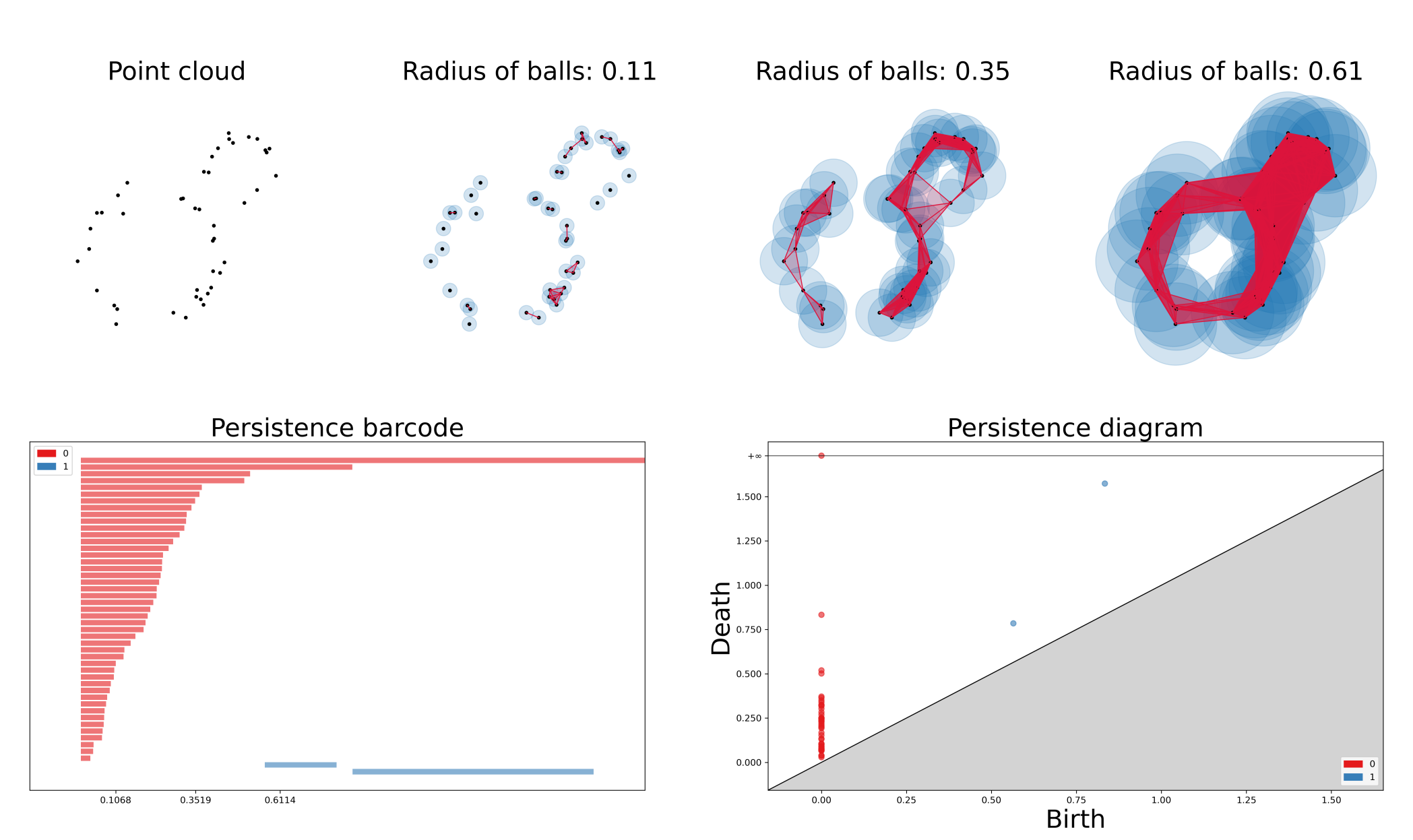
Figure 2: Vietoris–Rips filtration over two noisy circles (with 30 and 15 points each) at 4 different filtration values; and corresponding persistence barcode and diagram. Images produced using GUDHI [The GUDHI Project, 2020].

Appendix B Comparison of Spearman’s correlation for norm and PH dimension against generalization

In Section 4, we always observe stronger Spearman’s correlations between the norm and generalization compared to PH dimension and generalize. By using the Fisher’s z-tranformation we compare pairwise the difference in correlation coefficient. Table 5 emphasizes the significance of these differences. Note that a p-value less than 0.05 indicates significant differences, i.e. stronger correlations.

Table 5: P-values signifying significantly stronger correlation between the norm and generalization compared to PH dimension with generalization.

Model & Data	Euclidean PH dimension	Loss-based PH dimension
AlexNet & Cifar10	0	5.020e-13
FCN5 & MNIST	0	0
FCN5 & CHD	0	0
FCN7 & MNIST	0	0
FCN7 & CHD	0	1.763e-11

Appendix C Partial correlation

For comparison to the partial correlation computed between PH dimensions and generalization, we also the partial correlation between the norm and generalization. From Table 6, we observe significant partial correlation for models trained on CHD, and no significant partial correlation for the larger batch sizes for models trained on the MNIST dataset.

Table 6: Partial Spearman’s and Kendall correlation computed between the norm and generalization error for fixed batch sizes given learning rate.

		Partial correlation of norm with accuracy gap (or loss gap for regression) given learning rate
Model & Data	Batch size	Spearman’s correlation (p-value)	Kendall correlation (p-value)
FCN5 & MNIST	32	0.7788 (9.83e-13)	0.5713 (3.724e-10)
	76	0.6158 (3.434e-07)	0.4088 (7.173e-06)
	121	0.1622 (0.2279)	0.1129 (0.2153)
	166	-0.03870 (0.775)	-0.02320 (0.7989)
	211	-0.1222 (0.3654)	-0.07589 (0.4048)
	256	0.007451 (0.9565)	-0.003904 (0.9662)
FCN5 & CHD	32	-0.9113 (<2.2e-16)	-0.7671 (<2.2e-16)
	65	-0.8997 (<2.2e-16)	-0.7514 (<2.2e-16)
	99	-0.9037 (<2.2e-16)	-0.7525 (<2.2e-16)
	132	-0.8812 (<2.2e-16)	-0.7424 (<2.2e-16)
	166	-0.8912 (<2.2e-16)	-0.7480 (<2.2e-16)
	200	-0.9084 (<2.2e-16)	-0.7661 (<2.2e-16)
FCN7 & MNIST	32	0.4859 (8.293e-05)	0.3484 (8.526e-05)
	76	0.6966 (6.376e-10)	0.5205 (4.249e-09)
	121	0.4948 (5.847e-05)	0.3426 (0.000111)
	166	0.1657 (0.2058)	0.1166 (0.1888)
	211	-0.01673 (0.8991)	-0.01300 (0.8834)
	256	0.3152 (0.01418)	0.2092 (0.01828)
FCN7 & CHD	32	-0.7085 (<2.2e-16)	-0.5458 (7.225e-10)
	65	-0.7750 (<2.2e-16)	-0.6283 (2.066e-12)
	99	-0.8475 (<2.2e-16)	-0.6902 (1.135e-14)
	132	-0.7909 (<2.2e-16)	-0.6552 (3.737e-13)
	166	-0.9057 (<2.2e-16)	-0.7665 (<2.2e-16)
	200	-0.9272 (<2.2e-16)	-0.7992 (<2.2e-16)

Appendix D Conditional independence

For illustrative purposes, we present in Figures 3 and 4 the causal assumption for the null and alternative hypotheses.

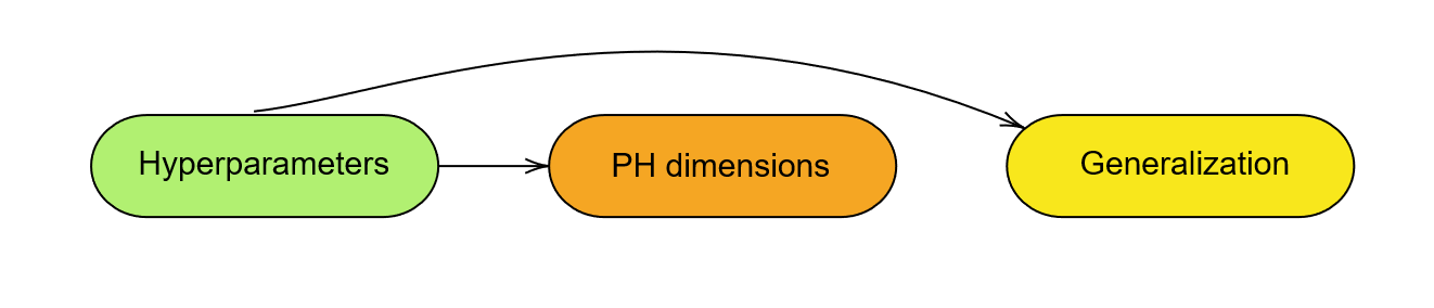
Figure 3: H0: There exists no causal link between PH dimensions and generalization – both are explained by the hyperparameters

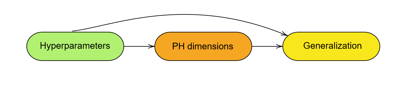
Figure 4: H1: Causal link between PH dimensions – generalization can be fully explained by PH dimensions

Appendix E Adversarial initialization

We provide an example of the contrasting correlation pattern between loss-based PH dimension and generalization for standard initialization and adversarial initialization shown in Figures 5 and 6.

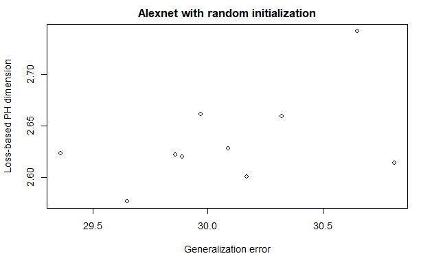
Figure 5: Positive correlation between loss-based PH dimension and generalization with standard initialization based on AlexNet model trained on CIFAR-10

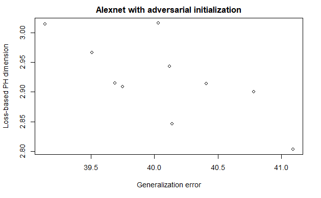
Figure 6: Negative correlation between loss-based PH dimension and generalization with adversarial initialization based on AlexNet model trained on CIFAR-10

References

- Adams et al. [2020] Henry Adams, Manuchehr Aminian, Elin Farnell, Michael Kirby, Joshua Mirth, Rachel Neville, Chris Peterson, and Clayton Shonkwiler. A Fractal Dimension for Measures via Persistent Homology. In Nils A. Baas, Gunnar E. Carlsson, Gereon Quick, Markus Szymik, and Marius Thaule, editors, Topological Data Analysis, Abel Symposia, pages 1–31, Cham, 2020. Springer International Publishing. ISBN 978-3-030-43408-3. doi: 10.1007/978-3-030-43408-3_1.
- Bartlett and Mendelson [2002] Peter L Bartlett and Shahar Mendelson. Rademacher and gaussian complexities: Risk bounds and structural results. Journal of Machine Learning Research, 3(Nov):463–482, 2002.
- Bauer [2021] Ulrich Bauer. Ripser: Efficient computation of Vietoris–Rips persistence barcodes. Journal of Applied and Computational Topology, 5(3):391–423, September 2021. ISSN 2367-1734. doi: 10.1007/s41468-021-00071-5.
- Bauer et al. [2014a] Ulrich Bauer, Michael Kerber, and Jan Reininghaus. Clear and compress: Computing persistent homology in chunks. In Topological Methods in Data Analysis and Visualization III: Theory, Algorithms, and Applications, pages 103–117. Springer, 2014a.
- Bauer et al. [2014b] Ulrich Bauer, Michael Kerber, and Jan Reininghaus. Distributed computation of persistent homology. In 2014 proceedings of the sixteenth workshop on algorithm engineering and experiments (ALENEX), pages 31–38. SIAM, 2014b.
- Birdal et al. [2021] Tolga Birdal, Aaron Lou, Leonidas J Guibas, and Umut Şimşekli. Intrinsic Dimension, Persistent Homology and Generalization in Neural Networks. In Advances in Neural Information Processing Systems, volume 34, pages 6776–6789. Curran Associates, Inc., 2021. URL https://proceedings.neurips.cc/paper/2021/hash/35a12c43227f217207d4e06ffefe39d3-Abstract.html.
- Camuto et al. [2021] Alexander Camuto, George Deligiannidis, Murat A. Erdogdu, Mert Gürbüzbalaban, Umut Şimşekli, and Lingjiong Zhu. Fractal Structure and Generalization Properties of Stochastic Optimization Algorithms, June 2021. URL http://arxiv.org/abs/2106.04881. arXiv:2106.04881 [cs, stat].
- Chen and Kerber [2011] Chao Chen and Michael Kerber. Persistent homology computation with a twist. In Proceedings 27th European workshop on computational geometry, volume 11, pages 197–200, 2011.
- Şimşekli et al. [2019] Umut Şimşekli, Mert Gürbüzbalaban, Thanh Huy Nguyen, Gaël Richard, and Levent Sagun. On the Heavy-Tailed Theory of Stochastic Gradient Descent for Deep Neural Networks, November 2019. URL http://arxiv.org/abs/1912.00018. arXiv:1912.00018 [cs, math, stat].
- Şimşekli et al. [2020] Umut Şimşekli, Ozan Sener, George Deligiannidis, and Murat A Erdogdu. Hausdorff Dimension, Heavy Tails, and Generalization in Neural Networks. In Advances in Neural Information Processing Systems, volume 33, pages 5138–5151. Curran Associates, Inc., 2020. URL https://papers.nips.cc/paper/2020/hash/37693cfc748049e45d87b8c7d8b9aacd-Abstract.html.
- Dupuis et al. [2023] Benjamin Dupuis, George Deligiannidis, and Umut Şimşekli. Generalization Bounds using Data-Dependent Fractal Dimensions. In Proceedings of the 40th International Conference on Machine Learning, pages 8922–8968. PMLR, July 2023. URL https://proceedings.mlr.press/v202/dupuis23a.html.
- Falconer [2007] Kenneth Falconer. Fractal geometry: mathematical foundations and applications. John Wiley & Sons, 2007.
- Guillou et al. [2023] Pierre Guillou, Jules Vidal, and Julien Tierny. Discrete morse sandwich: Fast computation of persistence diagrams for scalar data–an algorithm and a benchmark. IEEE Transactions on Visualization and Computer Graphics, 2023.
- Hastie et al. [2009] Trevor Hastie, Robert Tibshirani, Jerome H Friedman, and Jerome H Friedman. The elements of statistical learning: data mining, inference, and prediction, volume 2. Springer, 2009.
- He et al. [2019] Fengxiang He, Tongliang Liu, and Dacheng Tao. Control batch size and learning rate to generalize well: Theoretical and empirical evidence. In H. Wallach, H. Larochelle, A. Beygelzimer, F. d'Alché-Buc, E. Fox, and R. Garnett, editors, Advances in Neural Information Processing Systems, volume 32. Curran Associates, Inc., 2019. URL https://proceedings.neurips.cc/paper_files/paper/2019/file/dc6a70712a252123c40d2adba6a11d84-Paper.pdf.
- Jiang et al. [2019] Yiding Jiang, Behnam Neyshabur, Hossein Mobahi, Dilip Krishnan, and Samy Bengio. Fantastic Generalization Measures and Where to Find Them, December 2019. URL http://arxiv.org/abs/1912.02178. arXiv:1912.02178 [cs, stat].
- Kelley Pace and Barry [1997] R. Kelley Pace and Ronald Barry. Sparse spatial autoregressions. Statistics & Probability Letters, 33(3):291–297, May 1997. ISSN 0167-7152. doi: 10.1016/S0167-7152(96)00140-X.
- Kozma et al. [2005] Gady Kozma, Zvi Lotker, and Gideon Stupp. The minimal spanning tree and the upper box dimension. Proceedings of the American Mathematical Society, 134(4):1183–1187, September 2005. ISSN 0002-9939, 1088-6826. doi: 10.1090/S0002-9939-05-08061-5. URL http://arxiv.org/abs/math/0311481. arXiv:math/0311481.
- Krizhevsky [2009] Alex Krizhevsky. Learning Multiple Layers of Features from Tiny Images. 2009.
- Krizhevsky et al. [2017] Alex Krizhevsky, Ilya Sutskever, and Geoffrey E. Hinton. ImageNet classification with deep convolutional neural networks. volume 60, pages 84–90, May 2017. doi: 10.1145/3065386.
- Lecun et al. [1998] Y. Lecun, L. Bottou, Y. Bengio, and P. Haffner. Gradient-based learning applied to document recognition. Proceedings of the IEEE, 86(11):2278–2324, November 1998. ISSN 1558-2256. doi: 10.1109/5.726791.
- Liu et al. [2020] Shengchao Liu, Dimitris Papailiopoulos, and Dimitris Achlioptas. Bad global minima exist and sgd can reach them. Advances in Neural Information Processing Systems, 33:8543–8552, 2020.
- Myers and Sirois [2004] Leann Myers and Maria J Sirois. Spearman correlation coefficients, differences between. Encyclopedia of statistical sciences, 12, 2004.
- Nakkiran et al. [2021] Preetum Nakkiran, Gal Kaplun, Yamini Bansal, Tristan Yang, Boaz Barak, and Ilya Sutskever. Deep double descent: Where bigger models and more data hurt*. Journal of Statistical Mechanics: Theory and Experiment, 2021(12):124003, December 2021. ISSN 1742-5468. doi: 10.1088/1742-5468/ac3a74.
- Oudot [2017] Steve Y Oudot. Persistence theory: from quiver representations to data analysis, volume 209. American Mathematical Soc., 2017.
- Schweinhart [2020] Benjamin Schweinhart. Fractal dimension and the persistent homology of random geometric complexes. Advances in Mathematics, 372:107291, October 2020. ISSN 0001-8708. doi: 10.1016/j.aim.2020.107291. URL https://www.sciencedirect.com/science/article/pii/S0001870820303170.
- Schweinhart [2021] Benjamin Schweinhart. Persistent Homology and the Upper Box Dimension. Discrete & Computational Geometry, 65(2):331–364, March 2021. ISSN 1432-0444. doi: 10.1007/s00454-019-00145-3. URL https://doi.org/10.1007/s00454-019-00145-3.
- Tauzin et al. [2020] Guillaume Tauzin, Umberto Lupo, Lewis Tunstall, Julian Burella Pérez, Matteo Caorsi, Anibal Medina-Mardones, Alberto Dassatti, and Kathryn Hess. giotto-tda: A topological data analysis toolkit for machine learning and data exploration, 2020.
- The GUDHI Project [2020] The GUDHI Project. GUDHI User and Reference Manual. GUDHI Editorial Board, 3.1.1 edition, 2020. URL https://gudhi.inria.fr/doc/3.1.1/.
- Valle-Pérez and Louis [2020] Guillermo Valle-Pérez and Ard A. Louis. Generalization bounds for deep learning, December 2020. URL http://arxiv.org/abs/2012.04115. arXiv:2012.04115 [cs, stat].
- Vietoris [1927] L. Vietoris. Über den höheren Zusammenhang kompakter Räume und eine Klasse von zusammenhangstreuen Abbildungen. Mathematische Annalen, 97(1):454–472, December 1927. ISSN 1432-1807. doi: 10.1007/BF01447877. URL https://doi.org/10.1007/BF01447877.
- Xiao [2004] Yimin Xiao. Random fractals and markov processes. Fractal geometry and applications: a jubilee of Benoît Mandelbrot, 2:261–338, 2004.
- Zhang et al. [2021] Chiyuan Zhang, Samy Bengio, Moritz Hardt, Benjamin Recht, and Oriol Vinyals. Understanding deep learning (still) requires rethinking generalization. Communications of the ACM, 64(3):107–115, February 2021. ISSN 0001-0782. doi: 10.1145/3446776.
- Zomorodian and Carlsson [2005] Afra Zomorodian and Gunnar Carlsson. Computing Persistent Homology. Discrete & Computational Geometry, 33(2):249–274, February 2005. ISSN 1432-0444. doi: 10.1007/s00454-004-1146-y.