Enhancing the sensitivity of quantum fiber-optical gyroscopes via a non-Gaussian-state probe
Abstract
We propose a theoretical scheme to enhance the sensitivity of a quantum fiber-optical gyroscope (QFOG) via a non-Gaussian-state probe based on quadrature measurements of the optical field. The non-Gaussian-state probe utilizes the product state comprising a photon-added coherent state (PACS) with photon excitations and a coherent state CS. We study the sensitivity of the QFOG, and find that it can be significantly enhanced through increasing the photon excitations in the PACS probe. We investigate the influence of photon loss on the performance of QFOG and demonstrate that the PACS probe exhibits robust resistance to photon loss. Furthermore, we compare the performance of the QFOG using the PACS probe against two Gaussian-state probes: the CS probe and the squeezed state (SS) probe and indicate that the PACS probe offers a significant advantage in terms of sensitivity, regardless of photon loss, under the constraint condition of the same total number of input photons. Particularly, it is found that the sensitivity of the PACS probe can be three orders of magnitude higher than that of two Gaussian-state probes for certain values of the measured parameter. The capabilities of the non-Gaussian state probe on enhancing the sensitivity and resisting photon loss could have a wide-ranging impact on future high-performance QFOGs.
I Introduction
Enhancing the precision of measured parameters remains a fundamental topic in quantum metrology and quantum sensing 1Giovannetti ; 2Giovannetti ; 3Giovannetti ; 4Apellaniz ; 5Barbieri ; 6Degen ; 7Pirandola . Nonclassical effects of quantum systems 8Kwon can be used to improve the performance of various sensing systems beyond the shot noise limit that applies to classical sources. Quantum-enhanced metrology and sensing study how to exploit quantum resources to enhance the sensitivity of parameter estimations. It has already been demonstrated that squeezed states 9Caves ; 10LIGO ; 11Aasi ; 12LIGO ; 13Goodwin ; 14Ganapathy ; 15Anisimov ; 16Schnabel ; 17Zuo ; 18Zhao ; 19Pezz ; 20Nielsen , entangled states 21Zhang ; 22Wasilewski ; 23Zhao ; 24Belliardo ; 25Hao ; 26Boto ; 27Kok ; 28Joo ; 29Chen ; 30Maccone ; 31Li ; 32Zhuang ; 33Lloyd ; 34tTan ; 35Gallego ; 36Giovannetti ; 37Lee ; 38Joo ; 39Dowling , and quantum phase transitions 40Chen ; 41Chu ; 42Zhang ; 43Chu ; 44Lu ; 45Xu ; 46Jing ; 47Peng are important quantum resources that offer quantum advantages in many emerging sensing applications.
Recently, much attention has been paid to non-Gaussian states with Wigner negativity 48Walschaers ; 49Ra ; 50Melalkia due to theoretical and experimental progress in continuous-variable quantum information theory. Experimentally realizable non-Gaussian states include photon-added coherent (PAC) states 51Agarwal ; 52Zavatta ; 52Viciani ; 52Barbieri , Schrödinger cat states 53Ourjoumtsev ; 54Bao ; 55Wang ; 56Hacker ; 57Li ; 58Liu ; 59Huang ; 60Zou ; 61Liao ; 62Han ; 63Qin , and so on. Non-Gaussian states are widely applied in quantum information processing, such as quantum error correction 64Li ; 65Ofek ; 66Ma ; 67Schlegel , quantum metrology and quantum sensing 28Joo ; 29Chen ; 68Zhang ; 69Lee ; 70Zurek ; 71Gessner ; 72Tatsuta .
As is well known, the fiber-optic gyroscope (FOG) offers a high precision, compact solution for precision navigation in GPS denied environments, ultraprecise platform stabilization, and other inertial sensing applications 75Lefevre . The Quantum fiber optic gyroscope (QFOG) is a kind of quantum gyroscope that utilizes quantum resources such as quantum squeezing, quantum entanglement, and the non-Gaussianity of quantum states. 76Lenef ; 77Gustavson ; 78Wu2007 ; 79Canue ; 80Tackmann ; 81Stockton ; 82Savoie ; 83Dutta ; 84Avinadav ; 85Zhao ; 86Krzyzanowska ; 87Li2021 ; 88Li2018 ; 89Jiao ; 90Likai ; 91Li2023 ; 92LiG2022 ; 93Davuluri . The QFOG aims to realize rotation sensing with high precision by quantum effects. To date, however, studies on QFOGs have mainly focused on utilizing Gaussian states as quantum probes to improve the performance of the QFOG.
M. Mehmet and coworkers 94Mehmet demonstrated that the nonclassical sensitivity of the QFOG was improved by 4.5 dB beyond the shot-noise limit by the injection of squeezed light, and showed that the quantum enhancement of local area (kilometer-size) optical fiber networks and fiber-based measurement devices is feasible with squeezed light. Inspired by distributed quantum sensing schemes 95Zhuang ; 96Jacobs ; 97Proctor , M. R. Grace et al. 98Grace proposed an entanglement-enhanced QFOG that employs a stacked array of multiple identical Mach-Zehnder interferometers, with one part of a multimode-entangled squeezed vacuum state distributed to each.
In this paper, We propose a theoretical scheme to enhance the sensitivity of a quantum fiber-optical gyroscope (QFOG) via a non-Gaussian-state probe based on quadrature measurements of the optical field. The non-Gaussian-state probe utilizes the product state comprising a photon-added coherent state (PACS) with photon excitations and a coherent state CS. We study the sensitivity of the QFOG, and find that it can be significantly enhanced through increasing the photon excitations in the PACS probe. We investigate the influence of photon loss on the performance of QFOG and demonstrate that the PACS probe exhibits robust resistance to photon loss. Furthermore, we compare the performance of the QFOG using the PACS probe against two Gaussian-state probes: the CS probe and the squeezed state (SS) probe and indicate that the PACS probe offers a significant advantage in terms of sensitivity, regardless of photon loss, under the constraint condition of the same total number of input photons. Particularly, it is found that the sensitivity of the PACS probe can be three orders of magnitude higher than that of two Gaussian-state probes for certain values of the measured parameter. The capabilities of the non-Gaussian state probe on enhancing the sensitivity and resisting photon loss could have a wide-ranging impact on future high-performance QFOGs.
This paper is structured as follows. In Sec. II, we introduce the quadrature-measurement-based QFOG scheme and present a general expression to calculate its sensitivity. In Sec. III, we analyze the sensitivity of the QFOG when the two-mode probe is in a non-Gaussian state, which is a product state of a photon-added coherent state and a coherent state. In Sec. IV, we compare the sensitivity of the non-Gaussian-state probe with that of Gaussian-state probes and demonstrate the advantage of the non-Gaussian-state probe over the Gaussian-state probe under the same quantum resource conditions. Finally, our conclusions are summarized in Sec. V.
II Quadrature-measurement-based QFOG
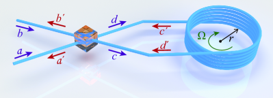
In this section, we describe the quadrature-measurement-based QFOG scheme and present a general expression to calculate the QFOG sensitivity. The QFOG under our consideration uses a Sagnac interferometer to measure angular velocity via the optical path delay induced in counterpropagating paths around a rotating loop as shown in Fig. 1. It consists of a lossless 50:50 beam splitter (BS) and a rotating optic-fiber loop. The quantum probe is the light state illuminating the gyroscope. Within the interferometer, the system is made of two counterpropagating modes and , that is the output modes of the BS. The output modes of the BS couple with the input modes through the following BS transformation
| (1) |
The propagation of the output modes of the BS within the fiber can be described by the unitary operator
| (2) |
where the phase is the Sagnac phase. It is proportional to the measured angular velocity with relationship where the scale factor is dependent on the optical center frequency of the laser, the number of fiber loops in the coil, the directed area of a single fiber loop.
The quadrature measurement will be made at the output modes and of the QFOG. These are related to the modes within the interferometer through the same BS performing the inverse transformation in Eq. (1)
| (3) |
Making use of Eqs. (1), (2), and (3), we can obtain the transformation relation between the input-output modes of the QFOG
| (4) |
Assuming symmetric loss processes that impose equal transmissivities on the two opposing paths around the fiber coil, we model fiber loss with the pure-loss channel
| (5) |
where and are two ancillary vacuum modes to describe photon loss in the two probe modes and of the QFOG, respectively. The parameter of modelling photon loss takes . implies no photon loss while denotes complete photon loss.
From Eqs. (4) and (5), we can obtain the transformation relation between the input and output modes of the QFOG in the presence of photon loss
| (6) | |||||
| (7) | |||||
In what follows, we investigate the sensitivity of the QFOG by using the quadrature measurement. For a boson field with the annihilation and creation operators and with the commutation relation , the quadrature operators are defined as
| (8) |
which satisfy the commutation relation .
For the output mode , making use of Eq. (7), we can obtain its quadrature operators
| (9) | ||||
| (10) |
Assuming that the two ancillary modes describing photon loss are in a vacuum state, we can obtain the variances of the quadrature operators of the mode from Eqs. (9) and (10)
| (11) | |||||
| (12) |
where the quadrature variances appeared in the right-hand side of above equations are calculated in the input states of the input modes and . In the derivation process of the variances of the quadrature operators of the mode, we have used the fact that the mean values of the quadrature operators of the two ancillary modes in a vacuum state vanish, and their variances are equal to .
The sensitivity of the QFOG based on the quadrature measurement can be expressed from the error transfer equation
| (13) |
Making use of the relation and Eqs. (9)-(12) we can find that the sensitivity of the QFOG is given by
| (14) | |||||
| (15) |
III The sensitivity of the QFOG with non-Gaussian-state probe
In this section, we study the sensitivity of the QFOG when the probe mode is in a photon-added coherent state while the probe mode is in a coherent state . We show that the sensitivity of the QFOG can be enhanced through increasing the number of photon excitations in the photon-added coherent state.
We consider a photon-added coherent state with excitations defined by
| (16) |
where is the normalization constant given by
| (17) |
with being the Laguerre polynomial defined by
| (18) |
We take the quadrature measurement of for the output mode of the QFOG. Assuming that both and are real numbers, from Eq. (15) we can find that the sensitivity of the QFOG is given by
| (19) |
where the mean value and variance of the quadrature operator in the PACS given by Eq. (16) are given by
| (20) | ||||
| (21) |
where -th order associated Laguerre polynomial defined by
| (22) |
From Eq. (19) we can observe that the sensitivity of the QFOG is independent of the state of the input mode . Then, we can take vacuum state as the state of the input mode to save quantum resource. Hence, the total number of photons in the input state of the QFOG is equal to that in the input mode of the PACS given by
| (23) |
However, the situation will change when we take as a real number, and a pure imaginary number ( is real). When the input state of the PACS probe is , the sensitivity of the QFOG (15) is reduced to
| (24) |
which indicates that the sensitivity of the QFOG depends on state parameters of the two input modes, and .
From Eqs. (19) and (24) we can also see that the smaller the photon loss rate , the larger the value of the sensitivity . Hence, the sensitivity of the QFOG deteriorates with the increase of photon loss. In the absence of photon loss (), the QFOG reaches the best sensitivity.
It is interesting to note that in the small rotation regime of , the QFOG has the same sensitivity for two different probe states and . In fact, we have and in the small rotation regime of , hence the sensitivity of the QFOG given by Eqs. (19) and (24) becomes the same expression
| (25) |
which implies that the sensitivity of the QFOG is independent of the measured parameter in the small rotation regime.
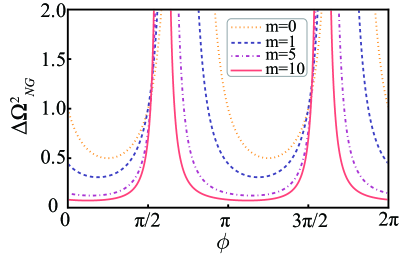
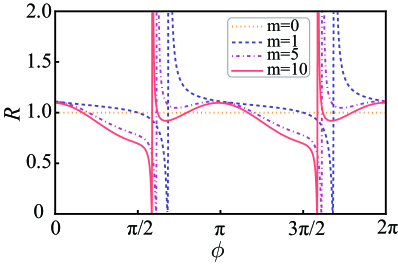
We now turn to the numerical investigation of the sensitivity of the QFOG. We only study the sensitivity of the QFOG based on the quadrature measurement given by Eq. (15) since the numerical results in next section indicate that the sensitivity of this case can surpass that of Gaussian-state probe. In Fig. 2 we plot the sensitivity of the QFOG with respect to the Sagnac phase in the absence of photon loss () when we take and for different excitation number and , respectively. Here the sensitivity is scaled by . From Fig. 2 we can see that (i) the sensitivity of the QFOG periodically changes with respect to the Sagnac phase. (ii) The QFOG can show high performance in most regime of one phase period. (iii) The values of the sensitivity decrease with the increase of the excitation number . Hence the performance of the QFOG is improved with the increase of the excitation number.
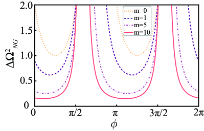
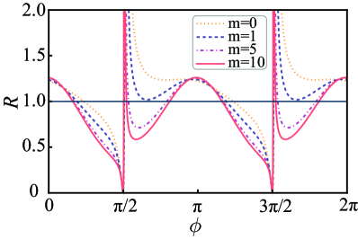
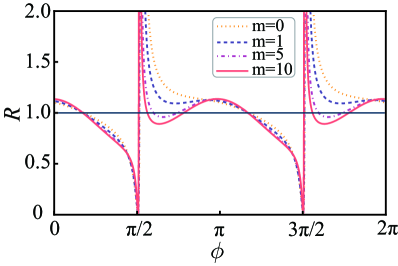
In Fig. 3 we plot the sensitivity of the QFOG with respect to the Sagnac phase in the presence of photon loss () when we take and for different excitation number and , respectively. From Fig. 3 we can find that quantum excitations of a coherent state can enhance the sensitivity of the QFOG even though there exists photon loss.
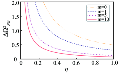
In order to further observe the influence of photon loss on the sensitivity, in Fig. 4 we show the sensitivity of the QFOG with respect to the photon loss when we take , , and for different excitation number and , respectively. From Fig. 4, we can see that the probe state with the larger excitation number exhibits the stronger ability against photon loss.
IV Comparison with the sensitivity of the QFOG with Gaussian-state probe
In this section, we compare the sensitivity of the non-Gaussian-state probe with that of Gaussian-state probes to show the advantage of the non-Gaussian-state probe over the Gaussian-state probe under the same condition of the quantum resource. We will consider two types of Gaussian-state probes. We regard the first Gaussian-state probe as the CS probe in which the input state of the probe is product of two coherent state with and being real. The second Gaussian-state probe is the squeezed-state probe in which the input state of the probe is product of a coherent state and a squeezed state with .
In order to study the advantage of the non-Gaussian probe over the Gaussian probe in the QFOG under the condition of the same input photon number, we introduce the ratio
| (26) |
where and are the sensitivity of the QFOG when the input state are non-Gaussian and Gaussian states, respectively. For the non-Gaussian probe with the input state , the sensitivity of the QFOG based on the quadrature measurement is given by Eq. (24). Therefore, means that the non-Gaussian QFOG has better sensitivity than the Gaussian QFOG.
IV.1 Comparison with the QFOG with coherent-state probe
For the coherent-state probe in which the input state of the QFOG is the product of two coherent states , the sensitivity of the QFOG based on the quadrature measurement can be obtained from Eq. (24) by setting and replacing with . We can find that the sensitivity of the QFOG with the CS probe is given by
| (27) |
From the constraint condition that the PACS probe and the CS probe have the same input photon number, we can obtain the following relation between state parameters of the PACS and CS probes
| (28) |
Making use of the sensitivity of the QFOG given by Eqs. (24) and (27), from Eq. (26) we can get the sensitivity ratio between the PACS and CS QFOG
| (29) |
where and are the expectation value and variance of the first quadrature operator of the probe mode in the PACS with photon excitations, they are have calculated in Eqs. (20) and (21).
In Fig. 5, we show the sensitivity ratio of the PACS and CS QFOG with respect to the Sagnac phase under the constraint of the same total number of input photons in the absence of photon loss () for different excitation numbers and , respectively. Here we take the probe parameters and . From Fig. 5 we can see that (i) the sensitivity of the QFOG periodically varies with respect to the Sagnac phase. (ii) The value of is less than unit in most regime of one phase period. This implies that the performance of the PACS QFOG is better than that of the CS QFOG in wide regime of one phase period. (iii) The values of the sensitivity ratio decrease with the increase of the excitation number . Hence quantum advantage of the PACS QFOG over the CS QFOG is more pronounced with the increase of the excitation number. (iv) There exists a best phase point at which the sensitivity ratio can suddenly change, and the PACS probe is significantly better than the CS probe. In fact, the further numerical analyse indicates that the sensitivity ratio of the PACS and CS QFOG can reach at the phase for photon excitations .
In Fig. 6, under the constraint of the same input mean photon number we plot the sensitivity ratio of the PACS and CS QFOG with respect to the Sagnac phase in the presence of photon loss () for different excitation numbers and , respectively. Here we also take the probe parameters and . Comparing Fig. 6 with Fig. 5 we can find that photon loss generally leads to narrowing the advantage range of the PACS probe with respect to the CS probe.
From the above numerical analyses we can conclude that the PACS probe can exhibit stronger quantum advantage in the phase estimation over the CS probe whether in the absence or presence of photon loss under the constraint condition of the same input mean photon number. Firstly, the higher excitation PACS probe can create better phase sensitivity limit than the CS probe. Secondly, the PACS probe has stronger capability against the photon loss. In particular, the PACS probe is significantly better than the CS probe at the best phase point.

IV.2 Comparison with the QFOG with squeezed-state probe
In this subsection, we make a comparison on the sensitivity of the QFOP between the non-Gaussian probe, the PACS probe, and the second kind of Gaussian probe, the squeezed-state probe. Assuming that the input state of the squeezed-state probe is the product of a coherent state and a squeezed state with the polarization decomposition of the squeezing parameter .
Based on the quadrature measurement, the sensitivity of the QFOG with the SS probe can be obtained from Eq. (24) with the following expression
| (30) |
where we have taken and used the following expect values and variances
| (31) | ||||
| (32) |
From the constraint condition that the PACS probe and the SS probe have the same input photon number, we can obtain the following relation between state parameters of the PACS and SS probes
| (33) |
from which we can obtain . Hence the state parameters of the SS probe can be expressed in terms of the state parameters of the PACS probe .
Making use of the sensitivity of the QFOG given by Eqs. (24) and (30), from Eq. (26) we can get the sensitivity ratio between the PACS and SS QFOG
| (34) |
where and are the expectation value and variance of the first quadrature operator of the probe mode in the PACS with photon excitations, they have been calculated in Eqs. (20) and (21).
In Fig. 7, we show the sensitivity ratio of the PACS and SS QFOG with respect to the Sagnac phase under the constraint of the same total number of input photons in the absence of photon loss () for different excitation numbers and , respectively. Here we take the probe parameters and . Fig. 7 indicates that when , the sensitivity ratio is less than unit in the phase regime of , and the larger the photon-excitation number , the smaller the sensitivity ratio . This implies that the sensitivity of the PACS QFOG is better than that of the SS QFOG, and the increase of the photon-excitation number can enhance the advantage of the PACS QFOG over the SS QFOG. When , we can find the second advantageous phase regime, , in which the sensitivity of the PACS QFOG is also better than that of the SS QFOG.
From Fig. 7 we can see that is the transition point of the sensitivity ratio at which the sensitivity ratio can suddenly change between and . In the small neighborhood on the left-hand side of the transition point, the PACS QFOG can exhibit the best advantage of the sensitivity over the SS QFOG. For example, from Fig. 7 we can find the sensitivity ratio of the PACS and SS QFOG can reach at the phase point for photon excitations .
In Fig. 8, we plot the sensitivity ratio of the PACS and CS QFOG with respect to the Sagnac phase under the constraint of the same input mean photon number in the presence of photon loss () for different excitation numbers and , respectively. Here we also take the probe parameters and . Comparing Fig. 8 with Fig. 7 we can find that photon loss suppress the advantage of the PACS-probe sensitivity with respect to the SS probe.
V Conclusions
In this work, we have proposed a theoretical scheme based on the quadrature measurement of the optical field to enhance the sensitivity of the QFOG via a non-Gaussian quantum probe. We constructed the QFOG quantum probe using the product state of the PACS with -photon excitations and the CS. We have studied the sensitivity of the QFOG using the non-Gaussian quantum probe , which highlights some relevant features of the QFOG. We have found that the sensitivity of the QFOG can be significantly enhanced by increasing the photon excitations in the PACS probe. We have also investigated the influence of photon loss on the performance of QFOG. It has been found that the probe state with higher excitation numbers exhibits stronger resistance to photon loss. The non-Gaussian-state offers two significant advantages over the Gaussian-state: enhanced sensitivity and robust resistance to photon loss. Furthermore, we have compared the performance of the QFOG using the PACS probe against the CS and SS probes by focusing on the sensitivity ratio. It has been demonstrated that the PACS probe can exhibit stronger quantum advantage in the sensitivity of QFOG over the CS and SS probes regardless of photon loss under the constraint condition of the same total number of input photons. In particular, it has been indicated that the sensitivity of the PACS probe can be three orders of magnitude higher than that of two Gaussian-state probes for certain values of the measured parameter. The capabilities of the non-Gaussian state probe in enhancing the sensitivity and resisting photon loss compared to Gaussian state probes could have a wide-ranging impact on future high-performance QFOGs.
Acknowledgements.
W. X. Zhang and R. Zhang are co-first authors with equal contribution to this work. L.-M. K. is supported by the Natural Science Foundation of China (NSFC) (Grant Nos. 12247105, 12175060, 11935006), Hunan provincial sci-tech program (Grant nos. 2020RC4047, 2023ZJ1010) and XJ-Lab key project (Grant No. 23XJ02001).References
- (1) V. Giovannetti, S. Lloyd, and L. Maccone, Advances in quantum metrology, Nat. Photon. 5, 222 (2011).
- (2) V. Giovannetti, S. Lloyd, and L. Maccone, Quantum enhanced measurements: Beating the standard quantum limit, Science 306, 1330 (2004).
- (3) V. Giovannetti, S. Lloyd, and L. Maccone, Quantum metrology, Phys. Rev. Lett. 96, 010401 (2006).
- (4) G. Tóth and I. Apellaniz, Quantum metrology from a quantum information science perspective, J. Phys. A 47, 424006 (2014).
- (5) M. Barbieri, Optical quantum metrology, PRX Quantum 3, 010202 (2022).
- (6) C. L. Degen, F. Reinhard, and P. Cappellaro, Quantum sensing, Rev. Mod. Phys. 89, 035002 (2017).
- (7) S. Pirandola, B. R. Bardhan, T. Gehring, C. Weedbrook, and S. Lloyd, Advances in photonic quantum sensing, Nat. Photon. 12, 724 (2018).
- (8) H. Kwon, K. C. Tan, T. Volkoff, and H. Jeong, Nonclassicality as a Quantifiable resource for quantum metrology, Phys. Rev. Lett. 122, 040503 (2019).
- (9) C. M. Caves, Quantum-mechanical noise in an interferometer, Phys. Rev. D 23, 1693 (1981).
- (10) The LIGO Scientific Collaboration, A gravitational wave observatory operating beyond the quantum shot-noise limit, Nat. Phys. 7, 962, 965 (2011).
- (11) J. Aasi, J. Abadie, B. Abbott et al., Enhanced sensitivity of the LIGO gravitational wave detector by using squeezed states of light, Nat. Photon. 7, 613,619 (2013).
- (12) LIGO Scientific Collaboration and V. Collaboration, Observation of Gravitational Waves from a Binary Black Hole Merger, Phys. Rev. Lett. 116, 061102 (2016).
- (13) A. W. Goodwin-Jones, R. Cabrita, M. Korobko, M. Van Beuzekom, D. D. Brown, V. Fafone, J. Van Heijningen, A. Rocchi, M. G. Schiworski, and M. Tacca, Transverse mode control in quantum enhanced interferometers: a review and recommendations for a new generation, Optica 11, 273 (2024).
- (14) D. Ganapathy et al., (LIGO O4 Detector Collaboration), Broadband Quantum Enhancement of the LIGO Detectors with Frequency-Dependent Squeezing, Phys. Rev. X 13, 041021 (2023).
- (15) P. M. Anisimov, G. M. Raterman, A. Chiruvelli, W. N. Plick, S. D. Huver, H. Lee, and J. P. Dowling, Quantum Metrology with Two-Mode Squeezed Vacuum: Parity Detection Beats the Heisenberg Limit, Phys. Rev. Lett. 104, 103602 (2010).
- (16) R. Schnabel, Squeezed states of light and their applications in laser interferometers, Phys. Rep. 648, 1 (2017).
- (17) X. Zuo, Z. Yan, Y. Feng, J. Ma, X. Jia, C. Xie, and K. Peng, Quantum Interferometer Combining Squeezing and Parametric Amplification, Phys. Rev. Lett. 124, 173602 (2020).
- (18) W. Zhao, S. D. Zhang, A. Miranowicz, and H. Jing, Weak-force sensing with squeezed optomechanics, Sci. China-Phys. Mech. Astron. 63, 224211 (2020).
- (19) L. Pezzé and A. Smerzi, Ultrasensitive Two-Mode Interferometry with Single-Mode Number Squeezing, Phys. Rev. Lett. 110, 163604 (2013).
- (20) J. A. H. Nielsen, J. S. Neergaard-Nielsen, T. Gehring, and U. L. Andersen, Deterministic Quantum Phase Estimation beyond N00N States, Phys. Rev. Lett. 130, 123603 (2023).
- (21) Z. Zhang, C. You, O. S. Magaña-Loaiza, R. Fickler, R. de J. León-Montiel, J. P. Torres, T. S. Humble, S. Liu, Y. Xia, and Q. Zhuang, Entanglement-based quantum information technology: a tutorial, Advances in Optics and Photonics 16, 60 (2024).
- (22) W. Wasilewski, K. Jensen, H. Krauter, J. J. Renema, M. V. Balabas, and E. S. Polzik, Quantum Noise Limited and Entanglement-Assisted Magnetometry, Phys. Rev. Lett. 104, 133601 (2010).
- (23) W. Zhao, X. Tang, X. Guo, X. Li, and Z. Y. Ou, Quantum entangled Sagnac interferometer, Appl. Phys. Lett. 122, 064003 (2023)
- (24) F. Belliardo and V. Giovannetti, Achieving Heisenberg scaling with maximally entangled states: An analytic upper bound for the attainable root-mean-square error, Phys. Rev. A 102, 042613 (2020).
- (25) S. Hao, H. Shi, C. N. Gagatsos, M. Mishra, B. Bash, I. Djordjevic, S. Guha, Q. Zhuang, and Z. Zhang, Demonstration of Entanglement-Enhanced Covert Sensing, Phys. Rev. Lett. 129, 010501 (2022).
- (26) A. N. Boto, P. Kok, D. S. Abrams, S. L. Braunstein, C. P. Williams, and J. P. Dowling, Quantum Interferometric Optical Lithography: Exploiting Entanglement to Beat the Diffraction Limit, Phys. Rev. Lett. 85, 2733 (2000).
- (27) P. Kok, A. N. Boto, D. S. Abrams, C. P. Williams, S. L. Braunstein, and J. P. Dowling, Quantum-interferometric optical lithography: Towards arbitrary two-dimensional patterns, Phys. Rev. A 63, 063407 (2001).
- (28) J. Joo, W. J. Munro, and T. P. Spiller, Quantum Metrology with Entangled Coherent States, Phys. Rev. Lett. 107, 083601 (2011).
- (29) X. T. Chen, R. Zhang, W. J. Lu, Y. L. Zuo, Y. F. Jiao, and L. M. Kuang, Asymmetry-enhanced phase sensing via asymmetric entangled coherent states, Phys. Rev. A 109, 042609 (2024)
- (30) L. Maccone and C. Ren, Quantum Radar, Phys. Rev. Lett. 124, 200503 (2020).
- (31) Y. Li and C. Ren, Entanglement-enhanced quantum strategies for accurate estimation of multibody-group motion and moving-object characteristics, Phys. Rev. A 108 062605 (2023).
- (32) Q. Zhuang, Quantum Ranging with Gaussian Entanglement, Phys. Rev. Lett. 126, 240501 (2021).
- (33) S. Lloyd, Enhanced sensitivity of photodetection via quantum illumination, Science 321, 1463 (2008).
- (34) S. H. Tan, B. I. Erkmen, V. Giovannetti, S. Guha, S. Lloyd, L. Maccone, S. Pirandola, and J. H. Shapiro, Quantum Illumination with Gaussian States, Phys. Rev. Lett. 101, 253601 (2008).
- (35) R. G. Torromè, Quantum Illumination with Multiple Entangled Photons, Adv. Quantum Tech. 4, 2100101 (2021)
- (36) G. V. Giovannetti, S. Lloyd, and L. Maccone, Quantum enhanced positioning and clock synchronization, Nature 412, 417 (2001).
- (37) S.-Y. Lee, Y. S. Ihn, and Z. Kim, Optimal entangled coherent states in lossy quantum-enhanced metrology, Phys. Rev. A 101, 012332 (2020).
- (38) J. Joo, K. Park, H. Jeong, W. J. Munro, K. Nemoto, and T. P. Spiller, Quantum metrology for nonlinear phase shifts with entangled coherent states, Phys. Rev. A 86, 043828 (2012).
- (39) J. P. Dowling, Quantum optical metrology - the lowdown on high-N00N states, Contemp. Phys. 49, 125 (2008).
- (40) C. Chen, P. Wang, and R.-B. Liu, Effects of local decoherence on quantum critical metrology, Phys. Rev. A 104, L020601 (2021).
- (41) Y. Chu, S. Zhang, B. Yu, and J. Cai, Dynamic Framework for Criticality-Enhanced Quantum Sensing, Phys. Rev. Lett. 126, 010502 (2021).
- (42) J. Zhang, Y. L. Zhou, Y. Zuo, H. Zhang, P. X. Chen, H. Jing, and L. M. Kuang, Exceptional Entanglement and Quantum Sensing with a Parity-Time-Symmetric Two-Qubit System, Adv. Quantum Tech. 2300350 (2024)
- (43) Y. Chu, Y. Liu, H. Liu, and J. Cai, Quantum Sensing with a Single-Qubit Pseudo-Hermitian System, Phys. Rev. Lett. 124, 020501 (2020).
- (44) H. Lü, S. K. Özdemir, L. M. Kuang, F. Nori, and H. Jing, Exceptional Points in Random-Defect Phonon Lasers, Phys. Rev. Applied 8, 044020 (2017).
- (45) X. W. Xu, J. Q. Liao, H. Jing, and L. M. Kuang, Anti-parity-time symmetry hidden in a damping linear resonator, Sci. China-Phys.-Mech.-Astron. 66, 100312 (2023).
- (46) H. Jing, H. Lü, Ş. K. Özdemir, T. Carmon, and F. Nori, Nanoparticle sensing with a spinning resonator, Optica 5, 1424 (2018).
- (47) Z. H. Peng, C. X.Jia, Y. Q. Zhang, Y. Yang, and L. M. Kuang, Single-lossy-nanoparticle sensor with a dissipatively coupled photonic molecule, Phys. Rev. A 108, 033716 (2023)
- (48) M. Walschaers, on-Gaussian quantum states and where to find them PRX Quantum 2, 030204 (2021).
- (49) Y.-S. Ra, A. Dufour, M. Walschaers, C. Jacquard, T. Michel, C. Fabre, and N. Treps, Non-Gaussian, quantum states of a multimode light field Nat. Phys. 16, 144 (2020).
- (50) M. F. Melalkia, J. Huynh, S. Tanzilli, V. D’Auria, and J. Etesse, A, multiplexed synthesizer for non-Gaussian photonic quantum state generation Quantum Sci. Technol. 8, 025007 (2023).
- (51) G. S. Agarwal and K. Tara, Nonclassical properties of states generated by the excitations on a coherent state, Phys. Rev. A 43, 492 (1991).
- (52) A. Zavatta, S. Viciani, and M. Bellini, Quantum-to-classical transition with single-photon-added coherent states of light, Science 306, 660 (2004).
- (53) A. Zavatta, S. Viciani, and M. Bellini, Single-photon excitation of a coherent state: Catching the elementary step of stimulated light emission, Phys. Rev. A 72, 023820 (2005).
- (54) M. Barbieri, N. Spagnolo, M. G. Genoni, F. Ferreyrol, R. Blandino, M. G. A. Paris, P. Grangier, and R. Tualle-Brouri, Non-Gaussianity of quantum states: An experimental test on single-photon-added coherent states, Phys. Rev. A 82, 063833 (2010).
- (55) A. Ourjoumtsev, H. Jeong, R. Tualle-Brouri, and P. Grangier, Generation of optical ¡®Schrödinger cats¡¯ from photon number states, Nature (London) 448, 784 (2007).
- (56) Z. Bao, Z. Wang, Y. Wu, Y. Li, W. Cai, W. Wang, Y. Ma, T. Cai, X. Han, J. Wang, Y. Song, L. Sun, H. Zhang, and L. Duan, Experimental preparation of generalized cat states for itinerant microwave photons Phys. Rev. A 105, 063717 (2022).
- (57) Z. Wang, Z. Bao, Y. Wu, Y. Li, W. Cai, W. Wang, Y. Ma, T. Cai, X. Han, J. Wang, Y. Song, L. Sun, H. Zhang, and L. Duan, A, flying Schrödinger cat in multipartite entangled states Sci. Adv. 8, eabn1778 (2022).
- (58) B. Hacker, S. Welte, S. Daiss, A. Shaukat, S. Ritter, L. Li, and G. Rempe, Deterministic creation of entangled atom¨Clight Schrödinger-cat states, Nat. Phtonics 13, 110 (2019).
- (59) B. Li, W. Qin, Y. F. Jiao, C. L. Zhai, X. W. Xu, L. M. Kuang, and H. Jing, Optomechanical Schrödinger cat states in a cavity Bose-Einstein condensate, Fundamental Research 3, 15 (2023).
- (60) J. Liu, Y. H. Zhou, J. Huang, J. F. Huang, and J. Q. Liao, Quantum simulation of a three-mode optomechanical system based on the Fredkin-type interaction, Phys. Rev. A 104, 053715 (2021).
- (61) J. Huang, Y. H. Liu, J. F. Huang, and J. Q. Liao, Generation of macroscopic entangled cat states in a longitudinally coupled cavity-QED model, Phys. Rev. A 101, 043841 (2020).
- (62) F. Zou, L. B. Fan, J. F. Huang, and J. Q. Liao, Enhancement of few-photon optomechanical effects with cross-Kerr nonlinearity, Phys. Rev. A 99, 043837(2019).
- (63) J. Q. Liao and L. Tian, Macroscopic Quantum Superposition in Cavity Optomechanics, Phys. Rev. Lett. 116, 163602 (2016).
- (64) D. M. Han, F. X. Sun, N. Wang, Y. Xiang, M. H. Wang, M. S. Tian, Q. Y. He, X. L. Su, Remote Preparation of Optical Cat States Based on Gaussian Entanglement, Laser & Photonics Reviews 2300103 (2023).
- (65) W. Qin, A. Miranowicz, H. Jing, and F. Nori, Generating Long-Lived Macroscopically Distinct Superposition States in Atomic Ensembles, Phys. Rev. Lett. 127, 093602 (2021)
- (66) L. Li, C. L. Zou, V. V. Albert, S. Muralidharan, S.M. Girvin, and L. Jiang, Cat Codes with Optimal Decoherence Suppression for a Lossy Bosonic Channel, Phys. Rev. Lett. 119, 030502 (2017).
- (67) N. Ofek, A. Petrenko, R. Heeres, P. Reinhold, Z. Leghtas, B. Vlastakis et al., Extending the lifetime of a quantum bit with error correction in superconducting circuits, Nature (London) 536, 441 (2016).
- (68) Y. Ma, Y. Xu, X. Mu, W. Cai, L. Hu, W. Wang, X. Pan, H. Wang, Y. Song, C.-L. Zou et al., Error-transparent operations on a logical qubit protected by quantum error correction, Nat. Phys. 16, 827 (2020).
- (69) D. S. Schlegel, F. Minganti, and V. Savona, Quantum error correction using squeezed Schrödinger cat states, Phys. Rev. A 106, 022431 (2022).
- (70) Y. M. Zhang, X. W. Li, W. Yang, and G. R. Jin, Quantum Fisher information of entangled coherent states in the presence of photon loss, Phys. Rev. A 88, 043832 (2013).
- (71) S.-Y. Lee, Y. S. Ihn, and Z. Kim, Optimal entangled coherent states in lossy quantum-enhanced metrology, Phys. Rev. A 101, 012332 (2020).
- (72) W. H. Zurek, Sub-Planck structure in phase space and its relevance for quantum decoherence, Nature (London) 412, 712 (2001).
- (73) M. Gessner, A. Smerzi, and L. Pezzé , Metrological Nonlinear Squeezing Parameter, Phys. Rev. Lett. 122, 090503 (2019).
- (74) M. Tatsuta, Y. Matsuzaki, and A. Shimizu, Quantum metrology with generalized cat states Phys. Rev. A 100, 032318 (2019).
- (75) H. C. Lefevre, The Fiber-Optic Gyroscope (Artech House, Boston, London, 2014), 2nd ed
- (76) A. Lenef, T. D. Hammond, E. T. Smith, M. S. Chapman, R. A. Rubenstein, and D. E. Pritchard, Rotation sensing with an atom interferometer, Phys. Rev. Lett. 78, 760 (1997).
- (77) T. L. Gustavson, P. Bouyer, and M. A. Kasevich, Precision rotation measurements with an atom interferometer gyroscope, Phys. Rev. Lett. 78, 2046 (1997).
- (78) S. Wu, Y.-J. Wang, Q. Diot, and M. Prentiss, Demonstration of an area-enclosing guided-atom interferometer for rotation sensing, Phys. Rev. Lett. 99, 173201 (2007).
- (79) B. Canuel, F. Leduc, D. Holleville, A. Gauguet, J. Fils, A. Virdis, A. Clairon, N. Dimarcq, Ch. J. Bordé, A. Landragin, and P. Bouyer, Six-axis inertial sensor using cold-atom interferometry, Phys. Rev. Lett. 97, 010402 (2005).
- (80) S. L. Christensen, J. B. Béguin, H. L .Sørensen, E. Bookjans, D. Oblak, J. H. Müller, J. Appel, and E. S. Polzik, Self-alignment of a compact large-area atomic Sagnac interferometer, N. J. Phys. 14, 015002 (2012).
- (81) J. K. Stockton, K. Takase, and M. A. Kasevich, Absolute geodetic rotation measurement using atom interferometry, Phys. Rev. Lett. 107, 133001 (2011).
- (82) D. Savoie, M. Altorio, B. Fang et al., Interleaved atom interferometry for high-sensitivity inertial measurements, Sci. Adv. 4, eaau7948 (2018).
- (83) I. Dutta, D. Savoie, B. Fang et al., Continuous cold-atom inertial sensor with 1 nrad/sec rotation stability[J]. Phys. Rev. Lett. 116, 183003 (2016).
- (84) C. Avinadav, D. Yankelev, M. Shuker et al., Rotation sensing with improved stability using point-source atom interferometry, Phys. Rev. A 102, 013326 (2020).
- (85) Y. Zhao, X. Yue, F. Chen et al., Extension of the rotation-rate measurement range with no sensitivity loss in a cold-atom gyroscope, Phys. Rev. A 104, 013312 (2021).
- (86) K. A. Krzyzanowska, J. Ferreras, C. Ryu, E. C. Samson, and M. G. Boshier, Matter-wave analog of a fiber-optic gyroscope, Phys. Rev. A 108, 043305 (2023).
- (87) B. B. Li, L. Ou, Y. Lei et al., Cavity optomechanical sensing, Nanophotonics, 10, 2799 (2021).
- (88) K. Li, S. Davuluri, and Y. Li, Improving optomechanical gyroscopes by coherent quantum noise cancellation processing, Science China Physics, Mechanics & Astronomy, 61, 1 (2018).
- (89) L. Jiao and J. H. An, Noisy quantum gyroscope, Photon. Res. 11, 150 (2023)
- (90) K. Li, S. Davuluri, and Y. Li, Three-mode optomechanical system for angular velocity detection, Chin. Phys. B 27, 084203 (2018).
- (91) H. Li and J. Cheng, Quantum estimation of rotational speed in optomechanics, Chin. Phys. B 32, 100602 (2023).
- (92) G.-L. Li, X. M. Lu, and X.-G. Wang et al., Optomechanical gyroscope simultaneously estimating the position of the rotation axis, JOSA B 39, 98 (2022).
- (93) D. Sankar, K. Li, and Y. Li, Gyroscope with two-dimensional optomechanical mirror, N. J. Phys. 19, 113004 (2017).
- (94) M. Mehmet, T. Eberle, S. Steinlechner, H. Vahlbruch, and R. Schnabel, Demonstration of a quantum-enhanced fiber Sagnac interferometer, Opt. Lett. 35, 1665 (2010).
- (95) Q. Zhuang, Z. Zhang, and J. H. Shapiro, Distributed quantum sensing using continuous-variable multipartite entanglement, Phys. Rev. A 97, 032329 (2018).
- (96) W. Ge, K. Jacobs, Z. Eldredge, A. V. Gorshkov, and M. Foss-Feig, Distributed Quantum Metrology with Linear Networks and Separable Inputs, Phys. Rev. Lett. 121, 043604 (2018).
- (97) T. J. Proctor, P. A. Knott, and J. A. Dunningham, Multiparameter Estimation in Networked Quantum Sensors, Phys. Rev. Lett. 120, 080501 (2018).
- (98) M. R. Grace, C. N. Gagatsos, Q. Zhuang, and S. Guha, Quantum-Enhanced Fiber-Optic Gyroscopes Using Quadrature Squeezing and Continuous-Variable Entanglement, Phys. Rev. Appl. 14, 034065 (2020).