Rectifying Reinforcement Learning
for Reward Matching

Abstract

The Generative Flow Network (GFlowNet) is a probabilistic framework in which an agent learns a stochastic policy and flow functions to sample objects with probability proportional to an unnormalized reward function. GFlowNets share a strong resemblance to reinforcement learning (RL), that typically aims to maximize reward, due to their sequential decision-making processes. Recent works have studied connections between GFlowNets and maximum entropy (MaxEnt) RL, which modifies the standard objective of RL agents by learning an entropy-regularized objective. However, a critical theoretical gap persists: despite the apparent similarities in their sequential decision-making nature, a direct link between GFlowNets and standard RL has yet to be discovered, while bridging this gap could further unlock the potential of both fields. In this paper, we establish a new connection between GFlowNets and policy evaluation for a uniform policy. Surprisingly, we find that the resulting value function for the uniform policy has a close relationship to the flows in GFlowNets. Leveraging these insights, we further propose a novel rectified policy evaluation (RPE) algorithm, which achieves the same reward-matching effect as GFlowNets, offering a new perspective. We compare RPE, MaxEnt RL, and GFlowNets in a number of benchmarks, and show that RPE achieves competitive results compared to previous approaches. This work sheds light on the previously unexplored connection between (non-MaxEnt) RL and GFlowNets, potentially opening new avenues for future research in both fields.

1 Introduction

Generative Flow Networks (GFlowNets) (Bengio et al., 2021, 2023) have emerged as a powerful probabilistic framework for object generation, which can be seen as a variant of amortized variational inference methods (Ganguly et al., 2022). In GFlowNets, an agent learns a stochastic policy and flow functions to sample objects proportionally to an unnormalized reward function. GFlowNets are related to Markov chain Monte Carlo (MCMC) methods (Metropolis et al., 1953, Hastings, 1970, Andrieu et al., 2003), but do not rely on Markov chains that make small and local steps. Therefore, they possess the ability to generalize and to amortize the cost of sampling without suffering from the mixing problem (Salakhutdinov, 2009, Bengio et al., 2013, 2021).

GFlowNets generate objects $x\in\mathcal{X}$ through a sequence of steps, where at each step the GFlowNets agent adds an element to the current construction. The sequential nature of GFlowNets bears a strong resemblance to the decision-making processes in reinforcement learning (RL) (Sutton and Barto, 2018). Indeed, the first GFlowNet training objective (Bengio et al., 2021) was motivated by the temporal difference methods in the RL (Sutton, 1988) literature. GFlowNets have achieved significant progress in various challenging problems, including drug discovery (Bengio et al., 2021), biological sequence design (Jain et al., 2022, Chen and Mauch, 2023), Bayesian structure learning (Deleu et al., 2022), combinatorial optimization (Zhang et al., 2024, 2023a), and large language models (Li et al., 2023, Hu et al., 2024).

Recent works have explored the connections between GFlowNets and maximum entropy (MaxEnt) RL (Tiapkin et al., 2024, Deleu et al., 2024, Mohammadpour et al., 2024), a variant of RL that modifies the standard objective by incorporating an entropy regularization term (Haarnoja et al., 2017b), which have provided valuable insights into the relationship between the two frameworks. However, establishing a direct link between GFlowNets and standard (non-MaxEnt) RL has remained elusive, despite the fact that both are based on sequential decision-making. The primary challenge in bridging this gap lies in the inherent differences in their objectives, as standard RL typically aims at reward maximization while GFlowNets aim at realizing reward matching. Despite these challenges, bridging this theoretical gap holds great promise, which could unlock new possibilities and further advance both fields.

In this paper, we uncover a new connection between GFlowNets and RL, based on policy evaluation for a uniform policy in RL. Surprisingly, we discover that the resulting value function for the uniform policy is closely associated with the flow functions in GFlowNets. Our findings bridge the gap between these two seemingly disparate frameworks, offering a more comprehensive understanding of their underlying and previously unexplored connections. Building upon this insight, we propose a novel rectified policy evaluation (RPE) algorithm for reward matching, which achieves the same effect as GFlowNets.

To validate our findings, we conduct extensive experiments in a number of evaluation benchmarks and compare GFlowNets (Bengio et al., 2021, Malkin et al., 2022, Bengio et al., 2023, Madan et al., 2023) with MaxEnt RL (Haarnoja et al., 2017a, Vieillard et al., 2020) and the RPE algorithm. Our results demonstrate that RPE achieves competitive performance compared to previous approaches, highlighting the effectiveness of our proposed method, and also sheds light on the previously unexplored connection between RL and GFlowNets.

2 Background

2.1 Generative Flow Networks

Consider a directed acyclic graph (DAG) $\mathcal{G}=\{\mathcal{S},\mathcal{A}\}$, where $\mathcal{S}$ and $\mathcal{A}$ represent the state and action spaces. The objective of GFlowNets is to learn a stochastic policy $\pi$ that constructs discrete objects $x\in\mathcal{X}$ with probability proportional to the reward function: $R$, i.e., $\pi(x)\propto R(x)$. The agent generates objects through a sequential process, and adds a new element to the current state at each timestep. The sequence of state transitions from the initial state to a terminal state is referred to as a trajectory, denoted by $\tau=(s_{0}\to...\to s_{n})$, where $\tau\in\mathcal{T}$ belongs to the set of all possible trajectories $\mathcal{T}$. Bengio et al. (2021) introduce the definition of the trajectory flow, represented by the function $F:\mathcal{T}\to\mathbb{R}_{\geq 0}$, which assigns a non-negative real value to each trajectory. The state flow, denoted by $F(s)$, is defined as the sum of flows of all trajectories passing through state $s$, i.e., $F(s)=\sum_{\tau\ni s}F(\tau)$. The edge flow $F(s\to s^{\prime})$ is the sum of flows of all trajectories containing the transition from state $s$ to state $s^{\prime}$, which is defined as $F(s\to s^{\prime})=\sum_{\tau\ni s\to s^{\prime}}F(\tau)$. We can then define the forward policy $P_{F}(s^{\prime}|s)={F(s\to s^{\prime})}/{F(s)}$, which determines the transition probabilities from a state $s$ to its possible children states $s^{\prime}$. In addition, we define the backward policy $P_{B}(s|s^{\prime})={F(s\to s^{\prime})}/{F(s)}$, which specifies the likelihood of reaching the parent state $s$ from the current state $s^{\prime}$. A flow is considered consistent if the total incoming flow for a state matches the total outgoing flow. It is proven in Bengio et al. (2021, 2023) that for consistent flows, the policy can sample objects $x$ with probability proportional to $R(x)$ and therefore match the underlying reward distribution.

Flow Matching (FM). Bengio et al. (2021) propose the flow matching to parameterize the edge flow function by $F_{\theta}(s,s^{\prime})$, with $\theta$ denoting the learnable parameters, which aims to optimize $F_{\theta}(s,s^{\prime})$ for satisfying the flow consistency constraint. The FM loss is defined as $\mathcal{L}_{\text{FM}}(s)=\left(\log\sum_{s^{\prime\prime}\to s}F_{\theta}(s^{\prime\prime},s)-\log\sum_{s\to s^{\prime}}F_{\theta}(s,s^{\prime})\right)^{2}$ for non-terminal states, which is the squared difference between the sum of incoming flows and the sum of outgoing flows. The term $\sum_{s\to s^{\prime}}F_{\theta}(s,s^{\prime})$ is replaced by $R(s)$ if $s$ is a terminal state. The loss is optimized in the log-scale due to stability issues.

(Sub) Trajectory Balance ((Sub)TB). Malkin et al. (2022) propose a trajectory-level optimization based on a telescoping calculation of detailed balance (DB) (Bengio et al., 2023), which is defined as $\mathcal{L}_{\text{TB}}(\tau)=(\log Z_{\theta}\prod_{t=0}^{n-1}P_{F_{\theta}}(s_{t+1}|s_{t}))-\log R(x)\prod_{t=0}^{n-1}P_{B_{\theta}}(s_{t}|s_{t+1}))^{2}$, that involves training the total flow $Z$, the forward and backward policies, but can lead to large variance. To mitigate the large variance problem of TB, SubTB (Madan et al., 2023) optimizes the flow consistency constraint in sub-trajectory levels. Specifically, it considers all possible $O(n^{2})$ sub-trajectories $\tau_{i:j}=\{s_{i},\cdots,s_{j}\}$, and obtain the objective defined as $\mathcal{L}_{\text{SubTB}}(\tau)=\sum_{\tau_{i:j}\in\tau}w_{ij}\left(\log F(s_{i})\prod_{t=i}^{j-1}P_{F}(s_{t+1}|s_{t})-\log F(s_{j})\prod_{t=i}^{j-1}P_{B}(s_{t}|s_{t+1})\right)^{2}$, where $w_{ij}$ represents the weight for $\tau_{i:j}$.

2.2 Reinforcement Learning (RL)

Algorithm 1 Policy Evaluation

0:  The policy $\pi$ to be evaluated; a small threshold $\theta$ for the accuracy of estimation

1:  Initialize value functions $V(s)$ arbitrarily for $s\in\mathcal{S}$, and $V(x)=R(x)$ for $x\in\mathcal{X}$

2:  repeat

3:     $\Delta\leftarrow 0$

4:     for $s\in\mathcal{S}\setminus\mathcal{X}$ do

5:        $v\leftarrow V(s)$

6:        $V(s)\leftarrow\sum_{a}\pi(a|s)(r+\gamma V(s^{\prime}))$

7:        $\Delta\leftarrow\max(\Delta,|v-V(s)|)$

8:  until $\Delta<\theta$

A Markov decision process (MDP) is defined as a $5$-tuple $(\mathcal{S},\mathcal{A},P,r,\gamma)$, where $\mathcal{S}$ represents the set of states, $\mathcal{A}$ represents the set of actions, $P:\mathcal{S}\times\mathcal{A}\to\mathcal{S}$ denotes the transition dynamics, $r$ is the reward function, and $\gamma$ is the discount factor. In an MDP, the RL agent interacts with the environment by following a policy $\pi$, which maps states to actions. The value function in a state $s$ for a policy $\pi$ is defined as the expected discounted cumulative reward the agent receives starting from the state $s$ , i.e., $V^{\pi}(s)=\mathbb{E}_{\pi}[\sum_{t=0}^{\infty}\gamma^{t}r(s_{t},a_{t})|s_{0}=s]$. The goal of RL is to find an optimal policy that maximizes the value function at all states. We consider the RL setting consistent with GFlowNets (as in Tiapkin et al. (2024)), with deterministic transitions and the discount factor to be $1$. It is worth noting that GFlowNets can also be extended to stochastic tasks (Pan et al., 2023b, Zhang et al., 2023b). In GFlowNets, the reward is obtained at the terminal state, while the reward typically occurs at transitions in RL. To bridge this gap, we define the value of terminal states $V(x)$ as $R(x)$.

Policy evaluation (Sutton and Barto, 1998) in the dynamic programming literature considers how to compute the value function for an arbitrary policy $\pi$, which is also referred to as the prediction problem. The iterative policy evaluation algorithm is summarized in Algorithm 1.

Maximum entropy RL. Maximum entropy RL (Neu et al., 2017, Haarnoja et al., 2017a, Geist et al., 2019) considers an entropy-regularized objective augmented by the Shannon entropy, i.e., $V^{\pi}_{\text{Soft}}(s)=\mathbb{E}_{\pi}[\sum_{t=0}^{\infty}\gamma^{t}r(s_{t},a_{t})+\lambda\mathcal{H}(\pi(s_{t}))|s_{t}=s]$, where $\lambda$ is the coefficient for entropy regularization. Schulman et al. (2017a) show that it corresponds to $Q_{\text{Soft}}^{*}(s,a)=r(s,a)+\gamma\mathbb{E}_{s^{\prime}\sim P(s,a)}[\lambda\log(\sum_{a^{\prime}}\exp(Q_{\text{Soft}^{*}}(s^{\prime},a^{\prime})/\lambda))]$, with the Boltzmann softmax policy $\pi_{\text{Soft}}^{*}(a|s)=\exp(\frac{1}{\lambda}Q^{*}_{\text{Soft}}(s,a)-V^{*}_{\text{Soft}}(s))$. Littman (1996) introduces the generalized Q-function, which considers using a generalized operator $\otimes$ for updating the Q-values, i.e., $Q(s,a)\leftarrow r(s,a)+\gamma\sum_{s^{\prime}\in\mathcal{S}}P(s^{\prime}|s,a)\otimes_{a^{\prime}}Q(s^{\prime},a^{\prime})$. Song et al. (2019), Pan et al. (2020b, a, 2021) study the Boltzmann softmax operator, defined as $\otimes_{a}Q(s,a)=\frac{\sum_{a}\exp(\beta Q(s,a))Q(s,a)}{\sum_{a}\exp{\beta Q(s,a)}}$, where $\beta$ denotes the temperature parameter. When $\beta$ approaches $\infty$, it corresponds to the max operator as typically used in standard Q-learning Mnih et al. (2013). On the other hand, when $\beta$ approaches $0$, it corresponds to the mean or average operator used in this paper. In this regard, MaxEnt RL can also be considered as a special extended case of a log-sum-exp operator while using Boltzmann softmax policy (Pan et al., 2020a).

3 Related Work

Generative Flow Networks (GFlowNets). Bengio et al. (2021) introduce Generative Flow Networks (GFlowNets) as a framework for learning stochastic policies that generate objects $x$ through a sequence of decision-making steps, aiming to sample $x$ with probability proportional to the reward function. GFlowNets have demonstrated remarkable success in various domains, including molecule generation (Bengio et al., 2021, Pan et al., 2022, lau2024qgfn), biological sequence design (Jain et al., 2022), Bayesian structure learning (Deleu et al., 2022), combinatorial optimization (Zhang et al., 2023a, 2024), and language models (Li et al., 2023, Hu et al., 2024), showcasing their potential for discovering high-quality and diverse solutions. Recent research has focused on providing theoretical understandings of GFlowNets by exploring their connections to variational inference (Zimmermann et al., 2022, Malkin et al., 2023), generative models Zhang et al. (2022), and Markov chain Monte Carlo methods (Deleu and Bengio, 2023). Temporal-difference methods in reinforcement learning (RL) (Sutton, 1988) serve as a significant inspiration for GFlowNets (Bengio et al., 2023). While recent works have drawn connections between GFlowNets and maximum entropy (MaxEnt) RL (Tiapkin et al., 2024, Mohammadpour et al., 2024, Deleu et al., 2024), they are limited to considering an entropy-regularized objective that differs from the goal of standard RL. This work establishes a direct link between GFlowNets and standard RL, aiming to bridge the gap between these two domains. By leveraging their inherent similarities in sequential decision-making, we revisit the standard RL algorithm and propose a novel approach to achieve the reward-matching objective.

Reinforcement Learning (RL). In RL, the problem is typically formulated as a Markov decision process (MDP) with states and actions defined similarly to the directed acyclic graph representation in GFlowNets. The agent learns a deterministic optimal policy to maximize the cumulative return (Sutton and Barto, 2018). Maximum-entropy (MaxEnt) RL (Haarnoja et al., 2017a), also known as soft RL or entropy-regularized RL, optimizes an entropy-regularized objective (Fox et al., 2015, Haarnoja et al., 2017b), where the agent seeks to maximize both the reward and action entropy, which falls under the broader domain of regularized MDPs (Neu et al., 2017, Geist et al., 2019). Soft Q-learning (Haarnoja et al., 2017b) is a popular instance of MaxEnt RL, which employs a log-sum-exp operator instead of the max operator commonly used in Q-learning (Mnih et al., 2013), along with a Boltzmann softmax policy (Schulman et al., 2017a, Pan et al., 2020a). Related studies have investigated alternative operators for learning the value function, demonstrating that the Boltzmann softmax operator (Song et al., 2019, Pan et al., 2020a) can mitigate the estimation bias (Pan et al., 2020a, 2021) in popular RL algorithms, when using a non-zero temperature parameter. Recently, Laidlaw et al. (2023) have shown that acting greedily with respect to the value function for a uniform policy can be as competitive as proximal policy optimization (PPO) (Schulman et al., 2017b) in several standard game environments. This finding highlights the potential of simple, uninformed learning strategies in achieving strong performance.

4 Rectifying Reinforcement Learning for Reward Matching

4.1 Prior Work

Previous works (Tiapkin et al., 2024, Deleu et al., 2024) have attempted to establish the connection of GFlowNets (Bengio et al., 2023) and maximum entropy RL (MaxEnt RL or soft RL;  Haarnoja et al. (2017b, 2018), Geist et al. (2019)), a variant of RL based on entropy-regularized objectives. Tiapkin et al. (2024) show that GFlowNets can be considered as MaxEnt RL with intermediate reward correction $r(s\to s^{\prime})=\log P_{B}(s|s^{\prime})$, where the soft value function $V_{\text{soft}}(s)$ corresponds to the logarithm of the state flows $F(s)$ in GFlowNets, i.e., $V_{\text{soft}}(s)=\log F(s)$. Similar connections also hold for the soft $Q$-function and the edge flow function. Despite these findings, the connection between GFlowNets and standard (non-MaxEnt) RL, i.e., RL using the Bellman operator (Sutton and Barto, 2018), remains unknown. In this paper, we aim to bridge this gap by establishing a direct link between these two frameworks, as both are formulated as sequential decision-making processes. Furthermore, we leverage the insights gained from this connection to rectify standard RL and propose a novel algorithm for achieving reward matching.

Algorithm 2 Flow Iteration

0:  The backward policy $P_{B}$ (e.g., uniform); a small threshold $\theta$ for estimation accuracy

1:  Initialize flow functions $F(s)$ arbitrarily for $s\in\mathcal{S}$, and $F(x)=R(x)$ for $x\in\mathcal{X}$

2:  repeat

3:     $\Delta\leftarrow 0$

4:     for $s\in\mathcal{S}\setminus\mathcal{X}$ do

5:        $f\leftarrow F(s)$

6:        $F(s)\leftarrow\sum_{s^{\prime}}P_{B}(s|s^{\prime})F(s^{\prime})$

7:        $\Delta\leftarrow\max(\Delta,|f-F(s)|)$

8:  until $\Delta<\theta$

4.2 Connecting GFlowNets and RL

To bridge the gap between GFlowNets and RL, we first establish the training of GFlowNets from a dynamic programming (DP) (Barto, 1995) perspective, which paves the way for understanding their relationship as many RL algorithms are based on the DP principles (Sutton and Barto, 1998).

We propose the Flow Iteration algorithm as outlined in Algorithm 2. Flow Iteration estimates the state flow $F(s)$ based on its possible children states and the backward policy (e.g., uniform), which is defined as $F(s)=\sum_{s^{\prime}}P_{B}(s^{\prime}|s)F(s^{\prime})$ (considering flow consistency in the state-edge level). The definition for state flows in GFlowNets is closely related to that of the state values in RL. Flow iteration considers a “backward” flow propagation, while policy evaluation (as introduced in Section 2.2) considers value propagation in a forward manner.

In the following sections, we investigate the relationship of RL and GFlowNets, starting with the simpler case of tree-structured graphs (Bengio et al., 2021) and then exploring the more challenging non-tree-structured directed acyclic graph (DAG) cases. Finally, we leverage these insights to develop a novel algorithm for rectifying RL to achieve the same goal as GFlowNets, i.e., sampling proportionally to the rewards.

4.2.1 Tree DAG

The state flow function $F(s)$ in GFlowNets and the state value function $V(s)$ in RL share an interesting connection when considering a uniform policy and a reward function scaled by the number of available actions in different states. Specifically, if we scale the original reward function $R(x)$ for a terminal state $x$ in GFlowNets by the product of the number of available actions in all the parent states leading to $x$, we observe an equivalence between $F(s)$ and $V(s)$. In Theorem 4.1, we restate and generalize the relationship between $V(s)$ (obtained by policy evaluation for a uniform policy) and $F(s)$, building upon and extending the initial observation made by Bengio et al. (2021).

Theorem 4.1 (Generalization of Bengio et al. (2021)[Proposition 4]).

For a GFlowNet that learns a state flow function $F(s_{t})$ and aims to sample proportionally from the reward function $R(x)$, it is equivalent to doing policy evaluation for a uniform policy $\pi(s^{\prime}|s)=\frac{1}{A(s)}$ whose value function $V(s_{t})=F(s_{t})\prod_{i=0}^{t-1}A(s_{i})$ models the scaled reward function $R^{\prime}(x)=R(x)\prod_{i=0}^{t-1}A(s_{i})$, where $A(s_{i})$ denotes the number of available actions at state $s_{i}$.

Remark. Therefore, there exists a close relationship between GFlowNets, standard (non-MaxEnt) RL, and MaxEnt RL, where the former is the focus of our work, and the latter has been established in a recent study (Tiapkin et al., 2024). GFlowNets can be associated with policy evaluation for a uniform policy with a transformed reward function. On the other hand, as RL aims to learn a reward-maximization policy, it also involves a process of policy improvement besides policy evaluation, which is referred to as policy iteration in dynamic programming (Sutton, 1988).

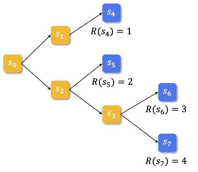
(a) Tree MDP.

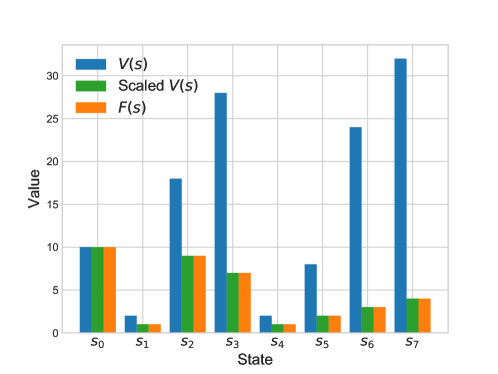
(b) Results of $F(s)$ and $V(s)$.

Figure 1: Comparison of policy evaluation and GFlowNets in a tree MDP example.

Empirical Validation. Consider the tree-structured DAG as shown in Figure 1(a), where the blue squares represent terminal states $x$ associated with rewards $R(x)$. To validate our theoretical findings, we compare the state flow function $F(s)$ in GFlowNets using the original reward function $R(x)$, with the state value function $V(s)$ for a uniform policy using transformed rewards $R^{\prime}(x)$. As demonstrated in Figure 1(b), we observe that the state flow function and the state value function for the initial state $s_{0}$ are identical, both providing an estimate of the total flow. For other states, we discover that by dividing the state value function $V(s)$ by the product of the number of available actions in the parent states of $s$, we obtain scaled $V(s)$ that are indeed equivalent to the state flow function $F(s)$. This provides a new perspective on how RL can be employed to achieve reward-matching (as opposed to the typical reward-maximization ability), in contrast to its typical reward-maximization capability. It is worth noting that different from (Tiapkin et al., 2024), we do not consider $\log P_{B}$ as intermediate rewards, but instead use a transformed terminal reward, where the scaling factor can be easily computed when we collect the trajectory. More details about the comparison results can be found in Appendix A.

4.2.2 Non-Tree DAG

Building upon the insights gained from the simpler tree case, we now study the more general and challenging setting of non-tree-structured DAGs.

In Theorem 4.2, we establish the connection between the state flow function in GFlowNets and the state value function in RL in non-tree DAG cases. The proof can be found in Appendix B due to the space limitation.

Theorem 4.2.

For a GFlowNet that learns a state flow function $F(s_{t})$ and aims to sample proportionally from the reward function $R(x)$, it is equivalent to doing policy evaluation for a uniform policy with the value function $V(s_{t})=F(s_{t})g(\tau,s_{t})$ modeling the reward function $R^{\prime}(x)=R(x)g(\tau,x)$, where $A(s_{i})$ denotes the number of available actions at state $s_{i}$, and $B(s_{i+1})$ denotes the number of incoming actions (parent nodes) at state $s_{i+1}$, and $g(\tau,s_{t})=\prod_{i=0}^{t-1}\frac{|A(s_{i})|}{|B(s_{i+1})|}$, if $s_{t}$ is a state in $\tau_{1}$ and $\tau_{2}$, we have that $g(\tau_{1},s_{t})=g(\tau_{2},s_{t})$, $\forall\tau_{1},\tau_{2}$.

Remark. Theorem 4.2 generalizes the relationship between GFlowNets and RL to non-tree DAG cases, where the state flow function $F(s)$ can be viewed as a scaled state value function $V(s)$ under a uniform policy with a transformed reward function. The scaling factor $g(\tau,s_{t})$ accounts for the number of available actions and incoming actions at each state along the trajectory. Different from the tree case which has no constraints, it needs to satisfy the condition that $g(\tau_{1},s_{t})=g(\tau_{2},s_{t})$ for any two trajectories $\tau_{1}$ and $\tau_{2}$ containing state $s_{t}$, which ensures the consistency of the same scaling factor across different paths leading to the same state.

It is worth noting that this assumption can be easily satisfied in a number of benchmark tasks for GFlowNets, e.g., the set generation task studied by Pan et al. (2023a) (where the number of available actions or parent states is independent of the state). However, there exist cases where this condition does not hold, e.g., HyperGrid (Bengio et al., 2021), where the presence of borders in the maze can sometimes lead to different $g$-values for the same state depending on the trajectory. We view this as a limitation of RL, since the equivalence between $F(s)$ and the scaled $V(s)$ can only be established when the assumption is satisfied, while GFlowNets can still achieve correct sampling in this case.

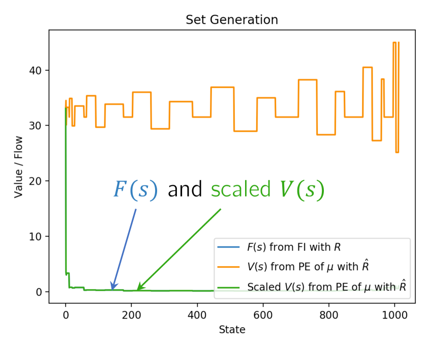
Figure 2: Comparison of policy evaluation and GFlowNets in the set generation task.

Empirical Validation. To validate this equivalence, we consider the small set generation task studied by Pan et al. (2023a). In this task, the agent sequentially generates a set with size $|S|$ from $|U|$ elements. At each timestep, the agent selects an element from $U$ and adds it to the current set (without replacement). The agent receives the reward for constructing the set with exactly $|S|$ elements. Figure 2 presents the results in the tabular case, where values or flows are represented in table form as the state and action spaces are enumerable. This tabular representation eliminates the influence of neural network approximation and sampling errors, providing a clear comparison between the state flow function and the scaled state value function. In Figure 2, the x-axis corresponds to different states, topologically sorted, and the y-axis corresponds to the value of $F$ or $V$. We show the results of policy evaluation with the transformed reward functions $R^{\prime}(x)$, policy evaluation with original rewards $R(x)$, and flow iteration. We observe that the scaled value function, denoted as scaled $V(s)$, coincides with the state flow function $F(s)$, validating the equivalence.

Algorithm 3 Rectified Policy Evaluation

0:  Flow function $F_{\theta}(s)$ parameterized by $\theta$, uniform policy $\pi$

0:  : Sampling policy $P_{F}(s^{\prime}|s)=\frac{F_{\theta}(s^{\prime})P_{B}(s|s^{\prime})}{F_{\theta}(s)}$ (a uniform $P_{B}$)

1:  for $t=\{1,\cdots,T\}$ do

2:     Sample a trajectory $\tau=\{s_{0},\cdots,s_{n}\}$ using $\pi$

3:     Calculate $g(s)$ for states $s\in\tau$

4:     for $s\in\tau$ do

5:        if s is not a terminal state then

6:           $V(s)\leftarrow\sum_{a}\pi(a|s)F_{\theta}(s^{\prime})g(s^{\prime})$

7:        else

8:           $V(s)\leftarrow g(s)R(s)$

9:     $\theta\leftarrow\arg\min\mathcal{L}_{\text{MSE}}(g(s)F_{\theta}(s),V(s))$ by an Adam optimizer

4.3 Rectified Reinforcement Learning for Reward Matching

Based on the above analysis, we propose to leverage the insights from the connections between flows and values to rectify policy evaluation with a uniform policy, which aims to learn a policy that samples proportionally to the rewards, similar to the objective of GFlowNets. The idea is summarized in Algorithm 3, which involves reparameterizing the value function $V(s)$ by $F(s)g(s)$, scaling the terminal rewards by the $g$-function, and doing simple policy evaluation for a uniform policy to obtain the same flow function as a GFlowNets. For simplicity, we consider a uniform backward policy $P_{B}$ for converting the flows into a forward policy for sampling, i.e., $P_{F}(s^{\prime}|s)=\frac{F(s^{\prime})P_{B}(s^{\prime}|s)}{F(s)}$.

As for estimating the value function under a uniform policy, it can also be considered as a mean operator, which is a special case of the Boltzmann softmax operator in RL (Song et al., 2019, Pan et al., 2020a, b, 2021) with a temperature of $0$. In contrast, the typical approach for employing the Boltzmann softmax operator for value function estimation in RL is to employ a non-zero temperature coefficient. This is because a temperature of $0$ leads to a mean operator that does not support maximization behavior, which is often a primary goal for RL agents. On the other hand, MaxEnt RL can be considered as using the log-sum-exp operator for estimating the value function with the Boltzmann softmax policy, as pointed out by Schulman et al. (2017a). This observation provides an intuitive connection of GFlowNets, MaxEnt RL, and RPE from the perspective of operators for value function estimation.

4.3.1 Discussion

In this section, we discuss the potential benefits of the RPE method , including a stable learning objective (and also reduced variance), simple parameterization, and a more informative sampling policy with improved generalization ability. These properties make RPE a promising approach to enhancing the performance and robustness of GFlowNets and related algorithms in a variety of settings. We experimentally validate the effect of RPE in Section 5.

Improved Learning Stability. In RPE, the policy to be evaluated is a fixed uniform policy $\pi$, which provides a more stable learning objective for the agent, compared to GFlowNets and MaxEnt RL approaches, which need to learn the flow functions or soft value functions for dynamically changing policies. Therefore, RPE is able to reduce the impact of policy non-stationarity on the learning process (although the sampling policy is still changing, evaluating a fixed policy mitigates one source of instability), thereby alleviating the moving target problem and related stability issues (Van Hasselt et al., 2018). It is worth noting that there is precedent for such an approach: Laidlaw et al. (2023) show that evaluating the uniform policy can be a powerful strategy in certain settings. Furthermore, when estimating the value function during training, RPE considers the value of all children states, which could potentially mitigate the problem of high variance (Van Seijen et al., 2009) typically encountered in GFlowNets within the trajectory balance (TB) objective (Malkin et al., 2022). By incorporating information from all possible next states, RPE can produce more stable and accurate value estimates.

A Simple Parameterization. In addition, RPE offers a simple parameterization, where the key component to be learned is the flow function $F_{\theta}$ only. Given a state $s\in\mathcal{S}$, what we need to predict is only a scalar. After obtaining $F_{\theta}$, the value function can be represented through Theorem 4.1 and Theorem 4.2, and the forward policy can be formulated as $F_{\theta}(s^{\prime})P_{B}(s^{\prime}|s)/F_{\theta}(s)$ with a specified $P_{B}$ (we use a uniform distribution). This simpler parameterization can reduce the approximation error induced by function approximators, and lead to more efficient learning properties (Shen et al., 2023).

An Informative Sampling Policy. RPE takes actions considering the flows of each next state, instead of directly learning a $\mathcal{S}\to\mathcal{A}$ mapping. As suggested by Shen et al. (2023), this approach provides better generalization ability by allowing the agent to “see" the child states. This enables the agent to make more informed decisions based on the properties of the states, and provides a better basis for an agent to take actions leading to states not encountered in training.

5 Experiments

In this section, we conduct extensive experiments to investigate the performance of GFlowNets, MaxEnt RL, and our rectified policy evaluation (RPE) algorithm, built on the connections we established in Section 4. We assess these algorithms using typical benchmarks for GFlowNets, including TFBind sequence generation (Shen et al., 2023), RNA sequence generation (Kim et al., 2023), and molecule generation (Shen et al., 2023).

5.1 Experimental Setup

Baselines. We compare RPE with GFlowNets with different learning objectives including Flow Matching (FM) (Bengio et al., 2021), Detailed Balance (DB) (Bengio et al., 2023), Trajectory Balance (TB) (Malkin et al., 2022), and Sub-Trajectory Balance (SubTB) (Madan et al., 2023) as introduced in Section 2.1. Additionally, we compare RPE with the maximum entropy (MaxEnt) RL algorithms, i.e., soft DQN (Haarnoja et al., 2017b) and Munchausen DQN (M-DQN;Vieillard et al. (2020), Tiapkin et al. (2024)), as described in Section 2.2.

Metrics. We evaluate each method in terms of the number of modes discovered during the course of training (Pan et al., 2023a), which measures the ability to identify multiple high-reward regions in the solution space. We also adopt the accuracy metric used in Shen et al. (2023) and Kim et al. (2023) for evaluation, which quantifies how well the learned policy distribution aligns with target reward distribution. Accuracy is calculated by computing the relative error between the sample mean of the reward function $R(x)$ under the learned policy distribution $P_{F}(x)$ and the expected value of $R(x)$ under the target distribution. The calculation of accuracy is given as $\text{Acc}(P_{F}(x))=100\times\min\left(\frac{\mathbb{E}_{P_{F}(x)}[R(x)]}{\mathbb{E}_{p^{*}(x)}[R(x)]},1\right)$, where $p^{*}(x)=R(x)/Z$ represents the target distribution.

Implementations. We implement all baselines based on open-source codes from Kim et al. (2023) and Tiapkin et al. (2024). It is also worth noting that we consider minimally modified transition dynamics that ensure the assumption required for GFlowNets and RL can be satisfied, while preserving the essential characteristics of the original tasks. We run each algorithm with three random seeds and report both the mean and standard deviation of their performance metrics. To ensure a fair comparison, all baselines use the same network architecture, batch size, and other relevant hyperparameters, with a more detailed description in Appendix C due to space limitation.

5.2 TF Bind Generation

We first explore the task of generating DNA sequences that exhibit high binding activity with human transcription factors (Jain et al., 2022) which are composed of $8$ nucleobases. The objective of the agent is to discover a diverse set of promising candidates that demonstrate strong binding affinity to the target transcription factor. At each timestep, the agent selects an amino acid $a$ and incorporates it into the currently generated partial sequence. We consider four reward functions from Lorenz et al. (2011).

We first study the task of a left-to-right generation of the TF Bind sequence as studied in  Malkin et al. (2022), where the agent chooses to append an amino acid $a$ to the end of the current state. This choice of constructive actions leads to a tree MDP, as each state only has one parent state. We then investigate the prepend-append MDP as introduced by Shen et al. (2023), where the actions involve prepending or appending a token $a$ to the current partial sequence. This formulation results in a more complex directed acyclic graph MDP, as opposed to a simple tree MDP, due to the existence of multiple trajectories for each object $x$, which poses significant challenges in the learning process.

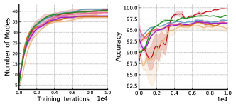
(a) TFbind 1 (Tree)

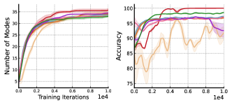
(b) TFBind 2 (Tree)

Figure 3: Number of modes discovered and accuracy over training across 3 random seeds.

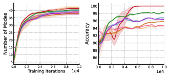
(a) TFBind 1 (DAG)

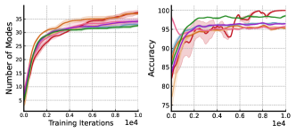
(b) TFBind 2 (DAG)

Figure 4: Number of modes discovered and accuracy of each method.

Figures 3-4 summarize the results in terms of accuracy and the number of modes discovered during training for each method, considering tree-structured generation and DAG-structured TF Bind generation, respectively. These figures present the results for two reward functions, while the complete results for all four reward functions can be found in Appendix D due to space constraints. As shown, GFlowNets (including FM, DB, TB, SubTB learning objectives), MaxEnt RL (including the popular Soft DQN algorithm and its GFlowNet-matching variant Munchausen DQN (Tiapkin et al., 2024)), and our RPE algorithm exhibit comparable performance in terms of the number of modes discovered, indicating their ability to effectively capture the multi-modal nature of the reward function. When considering accuracy, we observe that RPE generally outperforms other baselines by a small margin in the TF Bind generation tasks, where the most competitive baseline is M-DQN (Tiapkin et al., 2024), a variant of the Soft-DQN algorithm for MaxEnt RL. We believe this is because RPE can provide a more stable learning target, a simpler parameterization, a more informative sampling policy, and reduced variance, as discussed in §4.3.1.

5.3 RNA Sequence Generation

In this section, we study a larger practical task of generating RNA sequences composed of $14$ nucleobases. We consider four distinct target transcriptions employing the ViennaRNA package (Lorenz et al., 2011) as studied in Pan et al. (2024), where each task evaluates the binding energy with a unique target serving as the reward signal for the agent Lorenz et al. (2011). We follow the experimental setup as in Section 5.1, and study the prepend-append MDP introduced by Shen et al. (2023). More detailed descriptions of the setup can be found in Appendix C.

The performance of each method in terms of accuracy and the number of modes discovered for each task is shown in Figure 5. In this more challenging and larger task, we observe that RPE outperforms the baselines by a large margin, underscoring the efficiency of our method. RPE not only achieves the $100\%$ accuracy but also discovers the highest number of modes, showcasing its superior performance in both strong exploitation and exploration. This is relatively surprising, since the underlying mechanism of RPE is theoretically equivalent to GFlowNets that learn a state flow function $F(s)$. However, as we have previously speculated in §4.3.1, there may be certain advantages specific to RPE that contribute to its exceptional performance.

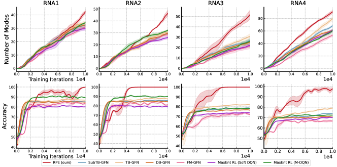
Figure 5: Top row: number of modes discovered over training across 3 random seeds. Bottom row: Accuracy over training across 3 random seeds.

5.4 Molecule Generation

In this section, we study the task of generating molecule graphs. We first study the QM9 molecule task as studied in prior GFlowNets work (Jain et al., 2023, Shen et al., 2023, Kim et al., 2023), where the reward function is defined as the energy gap between the highest occupied molecular orbital and lowest unoccupied orbital (HOMO-LUMO). We employ a pre-trained molecular property prediction model, MXMNet (Zhang et al., 2020), as the reward proxy. In addition, we study the sEH molecule generation task (Bengio et al., 2021), specifically the variant introduced by Shen et al. (2023), where the agent learns to design high-affinity ligands targeting the soluble epoxide hydrolase (sEH) protein. We use a pre-trained proxy model developed by Bengio et al. (2021).

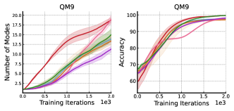
(a) QM9

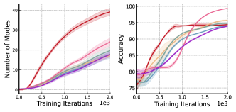
(b) sEH

Figure 6: Results in the molecule generation tasks.

The results for QM9 and sEH are summarized in Figure 6. RPE achieves consistent performance gain in the molecule generation tasks. Although RPE obtains a similar accuracy with baselines, it stands out for its accelerated mode detection. We find that the performance gap is larger for the more complex sEH task, where RPE discovers about $2\times$ more modes throughout training.

6 Conclusion

In this paper, we bridge the gap between GFlowNets and standard RL from the perspective of flow iteration and policy evaluation. Our results show that the resulting value function under a uniform policy shares close ties with flow functions in GFlowNets. Leveraging this insight, we then propose a novel algorithm named rectified policy evaluation (RPE) to facilitate a simple policy evaluation algorithm for reward matching. Empirical results on various standard benchmarks show that RPE performs better or competitively compared to both the GFlowNets methods and MaxEnt RL methods.

Appendix A Comparison of GFlowNets, MaxEnt RL and our results

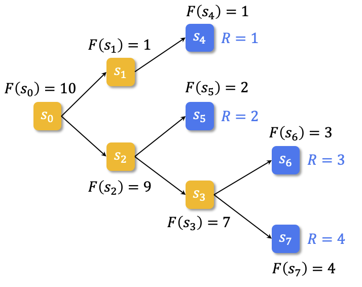
(a)

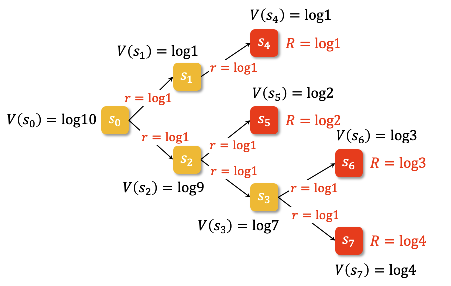
(b)

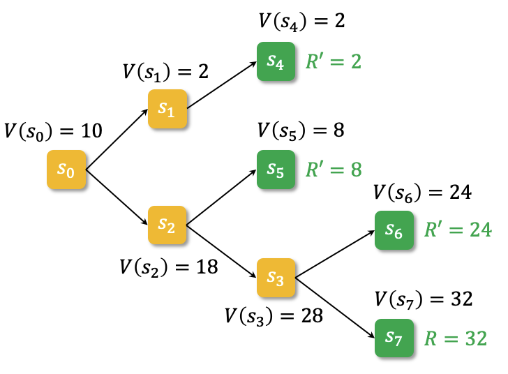
(c)

Figure 7: Illustration of flow and value for tree cases. (a) GFlowNets. (b) MaxEnt RL with intermediate reward correction. (c) Policy evaluation.

Appendix B Proofs

Theorem 4.2 For a GFlowNet that learns a state flow function $F(s_{t})$ and aims to sample proportionally from the reward function $R(x)$, it is equivalent to doing policy evaluation for a uniform policy with the value function $V(s_{t})=F(s_{t})g(\tau,s_{t})$ modeling the reward function $R^{\prime}(x)=R(x)g(\tau,x)$, where $A(s_{i})$ denotes the number of available actions at state $s_{i}$, and $B(s_{i+1})$ denotes the number of incoming actions (parent nodes) at state $s_{i+1}$, and $g(\tau,s_{t})=\prod_{i=0}^{t-1}\frac{|A(s_{i})|}{|B(s_{i+1})|}$, if $s_{t}$ is a state in $\tau_{1}$ and $\tau_{2}$, we have that $g(\tau_{1},s_{t})=g(\tau_{2},s_{t})$, $\forall\tau_{1},\tau_{2}$.

Proof.

It can be simply verified that the tree-structured DAG (Theorem 4.1) is a special case of the non-tree-structured DAG (Theorem 4.2), with $B(s_{i+1})=1$ and there is only one path from $s_{0}$ to any states. Therefore, we prove the general non-tree case here with mathematical induction (and the proof for Theorem 4.1 can be also obtained via the following proof since it is a special case).

For all terminal states $s_{n}$, by definition, we have that

$$V(s_{n})=R^{\prime}(s_{n})=R(s_{n})g(\tau,s_{n}).$$ (1)

$$F(s_{n})=R(s_{n}).$$ (2)

Thus, $V(s_{n})=F(s_{n})g(\tau,s_{n})$ holds for all terminal states.

Then, for any other state $s_{t}$, assume all of its children $s_{k}$ satisfy

$$V(s_{k})=F(s_{k})g(\tau,s_{k}).$$ (3)

By the definition of the policy evaluation procedure, we have that

$$V(s_{t})=\sum_{s_{t}\to s_{k}}\frac{V(s_{k})}{|A(s_{t})|}$$ (4)

Combining Eq.(3) and Eq.(4), we get

$$V(s_{t})=\sum_{s_{t}\to s_{k}}\frac{F(s_{k})g(\tau,s_{k})}{|A(s_{t})|}.$$ (5)

By definition, we have that

$$g(\tau,s_{k})=\prod_{i=0}^{k-1}\frac{|A(s_{i})|}{|B(s_{i+1})|}.$$ (6)

Thus, we obtain that

$$\frac{g(\tau,s_{k})}{|A(s_{t})|}=\frac{g(\tau,s_{k})}{|A(s_{k-1})|}=\frac{\prod_{i=0}^{k-2}|A(s_{i})|}{\prod_{i=0}^{k-1}|B(s_{i+1})|}=\frac{1}{|B(s_{k})|}\prod_{i=0}^{k-2}\frac{|A(s_{i})|}{|B(s_{i+1})|}.$$ (7)

As

$$g(\tau,s_{t})=g(\tau,s_{k-1})=\prod_{i=0}^{k-2}\frac{|A(s_{i})|}{|B(s_{i+1})|},$$ (8)

and combing Eq.(5),(7), and (8), we have that

$$V(s_{t})=\sum_{s_{t}\to s_{k}}\frac{F(s_{k})}{|B(s_{k})|}g(\tau,s_{t}).$$ (9)

By the definition of the flow iteration procedure, we have that

$$F(s_{t})=\sum_{s_{t}\to s_{k}}\frac{F(s_{k})}{|B(s_{k})|}.$$ (10)

Combing Eq.(9) and (10), we obtain that

$$V(s_{t})=F(s_{t})g(\tau,s_{t}).$$ (11)

Therefore, the condition holds for $s_{t}$. Finally, by induction, $V(s_{t})=F(s_{t})g(\tau,s_{t})$ holds for all states.

∎

Appendix C Experimental Setup

C.1 Implementation Details

We describe the implementation details of our method as follows:

• We use an MLP network that consists of 2 hidden layers with 2048 hidden units and ReLU activation (Xu et al., 2015) to estimate flow function $F_{\theta}$.

• we encode each state into a one-hot encoding vector and feed them into the MLP network.

• We clip gradient norms to a maximum of 10.0 to prevent unstable gradient updates.

• We run all the experiments in this paper on an RTX 3090 machine.

Below we introduce separate details for different benchmarks used in this paper.

TF Bind generation.

For the tree-structured TF Bind task, we follow the experimental setup described in Jain et al. (2022); For the graph-structured TF Bind task, we follow the experimental setup described in Shen et al. (2023). We select four tasks defined by different reward functions in Lorenz et al. (2011), i.e., SIX6_T165A_R1_8mers, ARX_P353L_R2_8mers, PAX3_Y90H_R1_8mers and WT1_REF_R1_8mers. In this task, we train our model for $1e^{4}$ steps, using the Adam optimizer Kingma and Ba (2014) with a $3e^{-3}$ learning rate. We set the reward threshold as 0.8 and the distance threshold as 3 to compute the number of modes discovered during training.

RNA Sequence generation.

We consider the PA-MDP to generate strings of 14 nucleobases. Following Pan et al. (2024), we present four different tasks characterized by different reward functions, i.e., RNA1, RNA2, RNA3 and RNA4. In this task, we train our model for $1e^{4}$ steps, using the Adam optimizer Kingma and Ba (2014) with a $3e^{-3}$ learning rate. We set the reward exponent as 3. We set the reward threshold as 0.8 and the distance threshold as 3 to compute the number of modes discovered during training. We normalize the reward into $[0.001,10]$ during training.

Molecule generation.

The goal of QM9 is to generate a molecule with 5 blocks from 12 building blocks with 2 stems. The goal of sEH is to generate a molecule with 6 blocks from 18 building blocks with 2 stems. Following the experimental setup described in Kim et al. (2023), we set the reward exponent as 5 for QM9, and 6 for sEH. In these 2 tasks, we train our model for $2e^{3}$ steps, using the Adam optimizer Kingma and Ba (2014) with a $1e^{-3}$ learning rate. To compute the number of modes discovered during training, we set the reward threshold as 6.5 and the distance threshold as 2 for sEH, and set the reward threshold as 1.4 and the distance threshold as 3 for QM9. We normalize the reward into $[0.001,1000]$ for QM9, and $[0.001,300]$ for sEH. This normalization is beneficial for flow regression.

Baselines.

We implement the MaxEnt RL baselines, including soft DQN and Munchausen DQN, by borrowing the code from https://github.com/d-tiapkin/gflownet-rl (Tiapkin et al., 2024). We implement the baselines of GFlowNets based on the codes from https://github.com/dbsxodud-11/ls_gfn (Kim et al., 2023).

Appendix D Additional Experimental Results

TF Bind

We provide the other two tasks of TF Bind generation benchmark in Fig 8. We find that RPE performs competitively in both tree and graph TFBind tasks.

RNA generation.

Table 1 and Table 2 summarize the results of the final model in the RNA generation tasks, which clearly show the superior performance of our method RPE in terms of both accuracy and number of modes discovered.

Baselines with uniform $P_{B}$.

Furthermore, we conduct a comparison between RPE and GFlowNets methods using a uniform $P_{B}$. As depicted in Fig. 9, the $P_{B}$ values in TB-GFN, SubTB-GFN, and DB-GFN are consistently fixed to be uniform. Our observations indicate that while these GFlowNets methods with uniform $P_{B}$ exhibit rapid convergence, they generally yield inferior performance compared to instances where $P_{B}$ is learned.

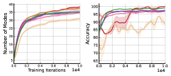
(a) Tree TFbind 3

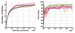
(b) Tree TFBind 4

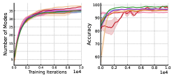
(c) Graph TFBind 3

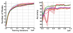
(d) Graph TFBind 4

Figure 8: Number of modes discovered and accuracy over training across 3 random seeds.

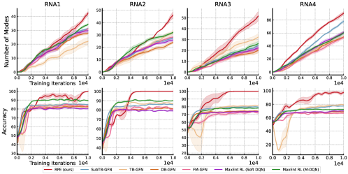
Figure 9: $P_{B}$ is fixed to be uniform for GFlowNets methods. Top row: number of modes discovered over training across 3 random seeds. Bottom row: Accuracy over training across 3 random seeds.

Table 1: Accuracy in different RNA generation tasks.

	L14_RNA1	L14_RNA2	L14_RNA3	L14_RNA4
FM-GFN	$83.54\pm 1.46$	$81.16\pm 1.03$	$71.82\pm 0.57$	$66.69\pm 1.13$
DB-GFN	$88.48\pm 0.41$	$88.49\pm 0.33$	$76.35\pm 0.44$	$70.53\pm 0.12$
TB-GFN	$86.81\pm 0.24$	$87.52\pm 0.18$	$81.80\pm 0.59$	$79.14\pm 0.78$
SubTB-GFN	$85.25\pm 0.46$	$86.67\pm 0.57$	$78.34\pm 0.67$	$74.10\pm 0.10$
MaxEnt RL (Soft DQN)	$80.27\pm 0.52$	$79.01\pm 0.03$	$73.52\pm 0.72$	$70.11\pm 1.13$
MaxEnt RL (M-DQN)	$89.55\pm 0.51$	$89.99\pm 0.43$	$78.28\pm 0.98$	$72.40\pm 0.73$
RPE (Ours)	$99.81\pm 0.19$	$100.0\pm 3.97$	$100.0\pm 2.45$	$97.68\pm 3.03$

Table 2: The number of modes discovered in different RNA generation tasks.

	L14_RNA1	L14_RNA2	L14_RNA3	L14_RNA4
FM-GFN	$31\pm 2$	$28\pm 2$	$21\pm 5$	$53\pm 5$
DB-GFN	$32\pm 4$	$30\pm 2$	$25\pm 4$	$61\pm 2$
TB-GFN	$34\pm 2$	$31\pm 2$	$31\pm 5$	$79\pm 7$
SubTB-GFN	$32\pm 3$	$29\pm 1$	$27\pm 4$	$68\pm 3$
MaxEnt RL (Soft DQN)	$30\pm 2$	$26\pm 2$	$22\pm 3$	$61\pm 5$
MaxEnt RL (M-DQN)	$34\pm 1$	$32\pm 1$	$22\pm 3$	$60\pm 5$
RPE (ours)	$42\pm 2$	$46\pm 6$	$52\pm 9$	$90\pm 6$

References

- Andrieu et al. (2003) Christophe Andrieu, Nando De Freitas, Arnaud Doucet, and Michael I Jordan. An introduction to mcmc for machine learning. Machine learning, 50:5–43, 2003.
- Barto (1995) Andrew G Barto. Reinforcement learning and dynamic programming. In Analysis, Design and Evaluation of Man–Machine Systems 1995, pages 407–412. Elsevier, 1995.
- Bengio et al. (2021) Emmanuel Bengio, Moksh Jain, Maksym Korablyov, Doina Precup, and Yoshua Bengio. Flow network based generative models for non-iterative diverse candidate generation. Advances in Neural Information Processing Systems, 34:27381–27394, 2021.
- Bengio et al. (2013) Yoshua Bengio, Grégoire Mesnil, Yann Dauphin, and Salah Rifai. Better mixing via deep representations. In International conference on machine learning, pages 552–560. PMLR, 2013.
- Bengio et al. (2023) Yoshua Bengio, Salem Lahlou, Tristan Deleu, Edward J Hu, Mo Tiwari, and Emmanuel Bengio. Gflownet foundations. Journal of Machine Learning Research, 24(210):1–55, 2023.
- Chen and Mauch (2023) Yihang Chen and Lukas Mauch. Order-preserving gflownets. arXiv preprint arXiv:2310.00386, 2023.
- Deleu and Bengio (2023) Tristan Deleu and Yoshua Bengio. Generative flow networks: a markov chain perspective. arXiv preprint arXiv:2307.01422, 2023.
- Deleu et al. (2022) Tristan Deleu, António Góis, Chris Emezue, Mansi Rankawat, Simon Lacoste-Julien, Stefan Bauer, and Yoshua Bengio. Bayesian structure learning with generative flow networks. In Uncertainty in Artificial Intelligence, pages 518–528. PMLR, 2022.
- Deleu et al. (2024) Tristan Deleu, Padideh Nouri, Nikolay Malkin, Doina Precup, and Yoshua Bengio. Discrete probabilistic inference as control in multi-path environments. arXiv preprint arXiv:2402.10309, 2024.
- Fox et al. (2015) Roy Fox, Ari Pakman, and Naftali Tishby. Taming the noise in reinforcement learning via soft updates. arXiv preprint arXiv:1512.08562, 2015.
- Ganguly et al. (2022) Ankush Ganguly, Sanjana Jain, and Ukrit Watchareeruetai. Amortized variational inference: Towards the mathematical foundation and review. arXiv preprint arXiv:2209.10888, 2022.
- Geist et al. (2019) Matthieu Geist, Bruno Scherrer, and Olivier Pietquin. A theory of regularized markov decision processes. In International Conference on Machine Learning, pages 2160–2169. PMLR, 2019.
- Haarnoja et al. (2017a) Tuomas Haarnoja, Haoran Tang, Pieter Abbeel, and Sergey Levine. Reinforcement learning with deep energy-based policies. In International conference on machine learning, pages 1352–1361. PMLR, 2017a.
- Haarnoja et al. (2017b) Tuomas Haarnoja, Haoran Tang, Pieter Abbeel, and Sergey Levine. Reinforcement learning with deep energy-based policies. In International conference on machine learning, pages 1352–1361. PMLR, 2017b.
- Haarnoja et al. (2018) Tuomas Haarnoja, Aurick Zhou, Pieter Abbeel, and Sergey Levine. Soft actor-critic: Off-policy maximum entropy deep reinforcement learning with a stochastic actor. In International conference on machine learning, pages 1861–1870. PMLR, 2018.
- Hastings (1970) W Keith Hastings. Monte carlo sampling methods using markov chains and their applications. 1970.
- Hu et al. (2024) Edward J Hu, Moksh Jain, Eric Elmoznino, Younesse Kaddar, Guillaume Lajoie, Yoshua Bengio, and Nikolay Malkin. Amortizing intractable inference in large language models. In The Twelfth International Conference on Learning Representations, 2024.
- Jain et al. (2022) Moksh Jain, Emmanuel Bengio, Alex Hernandez-Garcia, Jarrid Rector-Brooks, Bonaventure FP Dossou, Chanakya Ajit Ekbote, Jie Fu, Tianyu Zhang, Michael Kilgour, Dinghuai Zhang, et al. Biological sequence design with gflownets. In International Conference on Machine Learning, pages 9786–9801. PMLR, 2022.
- Jain et al. (2023) Moksh Jain, Sharath Chandra Raparthy, Alex Hernández-Garcıa, Jarrid Rector-Brooks, Yoshua Bengio, Santiago Miret, and Emmanuel Bengio. Multi-objective gflownets. In International conference on machine learning, pages 14631–14653. PMLR, 2023.
- Kim et al. (2023) Minsu Kim, Taeyoung Yun, Emmanuel Bengio, Dinghuai Zhang, Yoshua Bengio, Sungsoo Ahn, and Jinkyoo Park. Local search gflownets. In The Twelfth International Conference on Learning Representations, 2023.
- Kingma and Ba (2014) Diederik P Kingma and Jimmy Ba. Adam: A method for stochastic optimization. arXiv preprint arXiv:1412.6980, 2014.
- Laidlaw et al. (2023) Cassidy Laidlaw, Stuart J Russell, and Anca Dragan. Bridging rl theory and practice with the effective horizon. Advances in Neural Information Processing Systems, 36:58953–59007, 2023.
- Li et al. (2023) Yinchuan Li, Shuang Luo, Yunfeng Shao, and Jianye Hao. Gflownets with human feedback. arXiv preprint arXiv:2305.07036, 2023.
- Littman (1996) Michael Lederman Littman. Algorithms for sequential decision-making. Brown University, 1996.
- Lorenz et al. (2011) Ronny Lorenz, Stephan H Bernhart, Christian Höner zu Siederdissen, Hakim Tafer, Christoph Flamm, Peter F Stadler, and Ivo L Hofacker. Viennarna package 2.0. Algorithms for molecular biology, 6:1–14, 2011.
- Madan et al. (2023) Kanika Madan, Jarrid Rector-Brooks, Maksym Korablyov, Emmanuel Bengio, Moksh Jain, Andrei Cristian Nica, Tom Bosc, Yoshua Bengio, and Nikolay Malkin. Learning gflownets from partial episodes for improved convergence and stability. In International Conference on Machine Learning, pages 23467–23483. PMLR, 2023.
- Malkin et al. (2022) Nikolay Malkin, Moksh Jain, Emmanuel Bengio, Chen Sun, and Yoshua Bengio. Trajectory balance: Improved credit assignment in gflownets. Advances in Neural Information Processing Systems, 35:5955–5967, 2022.
- Malkin et al. (2023) Nikolay Malkin, Salem Lahlou, Tristan Deleu, Xu Ji, Edward J Hu, Katie E Everett, Dinghuai Zhang, and Yoshua Bengio. Gflownets and variational inference. In The Eleventh International Conference on Learning Representations, 2023.
- Metropolis et al. (1953) Nicholas Metropolis, Arianna W Rosenbluth, Marshall N Rosenbluth, Augusta H Teller, and Edward Teller. Equation of state calculations by fast computing machines. The journal of chemical physics, 21(6):1087–1092, 1953.
- Mnih et al. (2013) Volodymyr Mnih, Koray Kavukcuoglu, David Silver, Alex Graves, Ioannis Antonoglou, Daan Wierstra, and Martin Riedmiller. Playing atari with deep reinforcement learning. arXiv preprint arXiv:1312.5602, 2013.
- Mohammadpour et al. (2024) Sobhan Mohammadpour, Emmanuel Bengio, Emma Frejinger, and Pierre-Luc Bacon. Maximum entropy gflownets with soft q-learning. In International Conference on Artificial Intelligence and Statistics, pages 2593–2601. PMLR, 2024.
- Neu et al. (2017) Gergely Neu, Anders Jonsson, and Vicenç Gómez. A unified view of entropy-regularized markov decision processes. arXiv preprint arXiv:1705.07798, 2017.
- Pan et al. (2020a) Ling Pan, Qingpeng Cai, and Longbo Huang. Softmax deep double deterministic policy gradients. Advances in neural information processing systems, 33:11767–11777, 2020a.
- Pan et al. (2020b) Ling Pan, Qingpeng Cai, Qi Meng, Wei Chen, and Longbo Huang. Reinforcement learning with dynamic boltzmann softmax updates. In Christian Bessiere, editor, Proceedings of the Twenty-Ninth International Joint Conference on Artificial Intelligence, IJCAI-20, pages 1992–1998. International Joint Conferences on Artificial Intelligence Organization, 7 2020b. doi: 10.24963/ijcai.2020/276. URL https://doi.org/10.24963/ijcai.2020/276. Main track.
- Pan et al. (2021) Ling Pan, Tabish Rashid, Bei Peng, Longbo Huang, and Shimon Whiteson. Regularized softmax deep multi-agent q-learning. Advances in Neural Information Processing Systems, 34:1365–1377, 2021.
- Pan et al. (2022) Ling Pan, Dinghuai Zhang, Aaron Courville, Longbo Huang, and Yoshua Bengio. Generative augmented flow networks. In The Eleventh International Conference on Learning Representations, 2022.
- Pan et al. (2023a) Ling Pan, Nikolay Malkin, Dinghuai Zhang, and Yoshua Bengio. Better training of gflownets with local credit and incomplete trajectories. In International Conference on Machine Learning, pages 26878–26890. PMLR, 2023a.
- Pan et al. (2023b) Ling Pan, Dinghuai Zhang, Moksh Jain, Longbo Huang, and Yoshua Bengio. Stochastic generative flow networks. In Uncertainty in Artificial Intelligence, pages 1628–1638. PMLR, 2023b.
- Pan et al. (2024) Ling Pan, Moksh Jain, Kanika Madan, and Yoshua Bengio. Pre-training and fine-tuning generative flow networks. In The Twelfth International Conference on Learning Representations, 2024.
- Salakhutdinov (2009) Russ R Salakhutdinov. Learning in markov random fields using tempered transitions. Advances in neural information processing systems, 22, 2009.
- Schulman et al. (2017a) John Schulman, Xi Chen, and Pieter Abbeel. Equivalence between policy gradients and soft q-learning. arXiv preprint arXiv:1704.06440, 2017a.
- Schulman et al. (2017b) John Schulman, Filip Wolski, Prafulla Dhariwal, Alec Radford, and Oleg Klimov. Proximal policy optimization algorithms. arXiv preprint arXiv:1707.06347, 2017b.
- Shen et al. (2023) Max W Shen, Emmanuel Bengio, Ehsan Hajiramezanali, Andreas Loukas, Kyunghyun Cho, and Tommaso Biancalani. Towards understanding and improving gflownet training. In International Conference on Machine Learning, pages 30956–30975. PMLR, 2023.
- Song et al. (2019) Zhao Song, Ron Parr, and Lawrence Carin. Revisiting the softmax bellman operator: New benefits and new perspective. In International conference on machine learning, pages 5916–5925. PMLR, 2019.
- Sutton (1988) Richard S Sutton. Learning to predict by the methods of temporal differences. Machine learning, 3:9–44, 1988.
- Sutton and Barto (1998) Richard S Sutton and Andrew G Barto. Reinforcement learning: An introduction. 1998.
- Sutton and Barto (2018) Richard S Sutton and Andrew G Barto. Reinforcement learning: An introduction. MIT press, 2018.
- Tiapkin et al. (2024) Daniil Tiapkin, Nikita Morozov, Alexey Naumov, and Dmitry P Vetrov. Generative flow networks as entropy-regularized rl. In International Conference on Artificial Intelligence and Statistics, pages 4213–4221. PMLR, 2024.
- Van Hasselt et al. (2018) Hado Van Hasselt, Yotam Doron, Florian Strub, Matteo Hessel, Nicolas Sonnerat, and Joseph Modayil. Deep reinforcement learning and the deadly triad. arXiv preprint arXiv:1812.02648, 2018.
- Van Seijen et al. (2009) Harm Van Seijen, Hado Van Hasselt, Shimon Whiteson, and Marco Wiering. A theoretical and empirical analysis of expected sarsa. In 2009 ieee symposium on adaptive dynamic programming and reinforcement learning, pages 177–184. IEEE, 2009.
- Vieillard et al. (2020) Nino Vieillard, Olivier Pietquin, and Matthieu Geist. Munchausen reinforcement learning. Advances in Neural Information Processing Systems, 33:4235–4246, 2020.
- Xu et al. (2015) Bing Xu, Naiyan Wang, Tianqi Chen, and Mu Li. Empirical evaluation of rectified activations in convolutional network. arXiv preprint arXiv:1505.00853, 2015.
- Zhang et al. (2023a) David W Zhang, Corrado Rainone, Markus Peschl, and Roberto Bondesan. Robust scheduling with gflownets. arXiv preprint arXiv:2302.05446, 2023a.
- Zhang et al. (2022) Dinghuai Zhang, Ricky TQ Chen, Nikolay Malkin, and Yoshua Bengio. Unifying generative models with gflownets and beyond. arXiv preprint arXiv:2209.02606, 2022.
- Zhang et al. (2023b) Dinghuai Zhang, Ling Pan, Ricky TQ Chen, Aaron Courville, and Yoshua Bengio. Distributional gflownets with quantile flows. arXiv preprint arXiv:2302.05793, 2023b.
- Zhang et al. (2024) Dinghuai Zhang, Hanjun Dai, Nikolay Malkin, Aaron C Courville, Yoshua Bengio, and Ling Pan. Let the flows tell: Solving graph combinatorial problems with gflownets. Advances in Neural Information Processing Systems, 36, 2024.
- Zhang et al. (2020) Shuo Zhang, Yang Liu, and Lei Xie. Molecular mechanics-driven graph neural network with multiplex graph for molecular structures. arXiv preprint arXiv:2011.07457, 2020.
- Zimmermann et al. (2022) Heiko Zimmermann, Fredrik Lindsten, Jan-Willem van de Meent, and Christian A Naesseth. A variational perspective on generative flow networks. arXiv preprint arXiv:2210.07992, 2022.