On The Statistical Representation Properties Of The Perturb-Softmax And The Perturb-Argmax Probability Distributions
Abstract
The Gumbel-Softmax probability distribution allows learning discrete tokens in generative learning, while the Gumbel-Argmax probability distribution is useful in learning discrete structures in discriminative learning. Despite the efforts invested in optimizing these probability models, their statistical properties are under-explored. In this work, we investigate their representation properties and determine for which families of parameters these probability distributions are complete, i.e., can represent any probability distribution, and minimal, i.e., can represent a probability distribution uniquely. We rely on convexity and differentiability to determine these statistical conditions and extend this framework to general probability models, such as Gaussian-Softmax and Gaussian-Argmax. We experimentally validate the qualities of these extensions, which enjoy a faster convergence rate. We conclude the analysis by identifying two sets of parameters that satisfy these assumptions and thus admit a complete and minimal representation. Our contribution is theoretical with supporting practical evaluation.
1 Introduction
Learning over discrete probabilistic models is an active research field with numerous applications. Examples include learning probabilistic latent representations of semantic classes or beliefs (Kingma et al., 2014; Mnih & Gregor, 2014; Salakhutdinov & Hinton, 2009). The Gumbel-Argmax and Gumbel-Softmax probability distributions are widely applied in machine learning to model and analyze discrete probability distributions.
The Gumbel-Argmax is an equivalent representation of the softmax operation and plays a key role in “follow the perturb-leader” family of algorithms in online learning (Hannan, 1957; Kalai & Vempala, 2002, 2005; Rakhlin et al., 2012). Its extension to Gaussian-Argmax allows better bounds on their gradients and consequently provides better regret bounds in linear and high-dimensional settings Abernethy et al. (2014, 2016); Cohen & Hazan (2015). The argmax operation allows for efficient sampling, making the Perturb-Argmax probability models pivotal in discriminative learning algorithms of high-dimensional discrete structures (Berthet et al., 2020; Pogančić et al., 2020; Song et al., 2016; Cohen Indelman & Hazan, 2021; Niculae et al., 2018). The Gumbel-Softmax (or the Concrete distribution) probability distribution, which replaces the argmax operation with a softmax operation is easier to optimize and therefore plays a key role in generative learning models (Jang et al., 2017; Maddison et al., 2017). The discrete nature of these probability models provides a natural representation of concepts, e.g., in zero-shot text-to-image generation (DALL-E) (Ramesh et al., 2021). While the Gumbel-Argmax and Gumbel-Softmax probability distributions are widely applied in machine learning, their statistical representation is still under-explored.
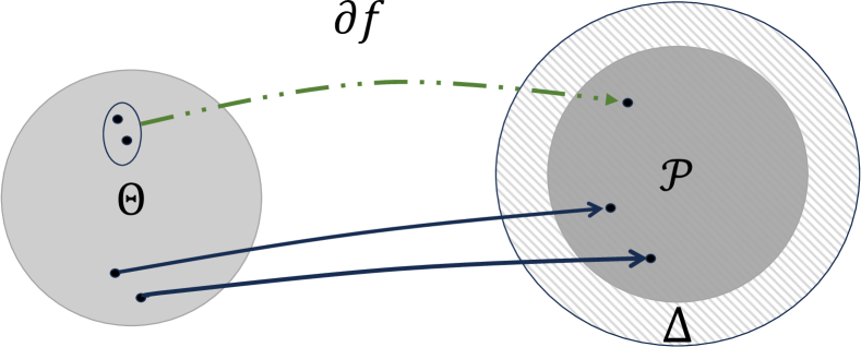
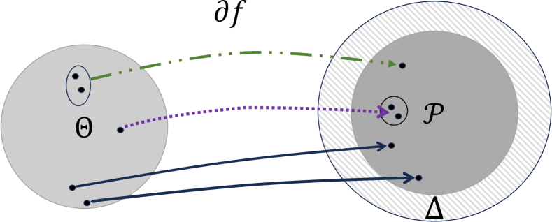
In this work, we investigate the representation properties of the Gumbel-Argmax and Gumbel-Softmax probability distributions. We aim to determine for which families of parameters these distributions are complete and minimal. A distribution is considered complete if it can represent any probability distribution, and minimal if it can uniquely represent a probability distribution. Our statistical investigation realizes the Gumbel-Argmax and the Gumbel-Softmax probability distributions as gradients of respective convex functions. In Theorems 4.1 and 4.3, we prove the conditions under which is a complete and minimal representation of the Gumbel-Softmax probability distribution and generalize these results to other random perturbations, e.g., Gaussian-Softmax or more generally, Perturb-Softmax probability distributions. We also extend these methods to Perturb-Argmax probability distributions, for which Gumbel-Argmax is a special case, and state the conditions for which it is complete and minimal in Theorems 5.1 and 5.3. Our findings are illustrated in Figure 1.
We begin by introducing the notation relating parameters and the relevant probability distributions in Section 3. Subsequently, we investigate the Perturb-Softmax probability models as gradients of the expected log-sum-exp convex function and prove their completeness by connecting their gradients to the relative interior of the probability simplex. In Section 4, we determine the minimality of Perturb-Softmax by the strict convexity of the expected log-sum-exp when restricted to the respective parameter space. We then investigate the Perturb-Argmax probability models as sub-gradients of the expected-max convex function and establish the conditions for which their parameter space is complete and minimal, see Section 5. Finally, we empirically demonstrate the qualities of Perturb-Softmax extension in generative and discriminative learning setting, showing improved convergence of Gaussian-Softmax over Gumbel-Softmax beyond the linear high-dimensional setting that was investigated in online learning Abernethy et al. (2014); Cohen & Hazan (2015).
2 Related work
The exponential family realized by the softmax operation over its parameters is extensively used in machine learning. However, sampling high-dimensional models is challenging due to its normalizing factor (Geman & Geman, 1984; Goldberg & Jerrum, 2007). The Gumbel-Argmax probability distribution measures the stability of the argmax operation over Gumbel random variables. It serves as an equivalent representation of softmax operation, thereby enabling efficient sampling from the exponential family (Gumbel, 1954; Luce, 1959). In the context of machine learning, the Gumbel-Argmax probability models underlie the ”follow the perturbed-leader” online learning algorithm (Hannan, 1957; Kalai & Vempala, 2002, 2005). The Gaussian-Argmax probability models extend the ”follow the perturbed-leader” family of online algorithms and improve their regret bounds (Rakhlin et al., 2012; Abernethy et al., 2014, 2016; Cohen & Hazan, 2015). Our work complements these studies by exploring the statistical properties of Gumbel-Argmax and Gaussian-Argmax. We prove the conditions under which Perturb-Argmax probability models are complete, making them suitable for use in machine learning, and when they are minimal, meaning they can uniquely identify a probability distribution from Perturb-Argmax probability models.
The Gumbel-Softmax probability models were introduced as an alternative to the exponential family and its Gumbel-Argmax equivalent in the context of generative learning (Maddison et al., 2017; Jang et al., 2017). This alternative allows for efficient sampling, making it highly effective for learning with stochastic gradient methods. The discrete nature of the Gumbel-Softmax sampling has been utilized to tokenize the visual vocabulary in the celebrated zero-shot text-to-image generation, DALL-E (Ramesh et al., 2021). The Gaussian-Softmax probability models were introduced in variational auto-encoders as their closed-form KL-divergence makes it easier to realize as regularization (Potapczynski et al., 2020). Our work extends these works and sets the statistical properties of Gumbel-Softmax and Gaussian-Softmax. We also show that Gaussian-Softmax enjoys faster convergence as the Gaussian distribution decays faster than the Gumbel distribution when approaching infinity.
Berthet et al. (2020) introduced a framework for optimizing discrete problems based on Perturb-Argmax probability models. This framework applies to discriminative learning using the Fenchel-Young losses and relies on convexity to propagate gradients over discrete choices. Similar to our approach, this work adopts a general view and utilizes convexity to explore the gradient properties of Perturb-Argmax models. Our work differs in that we use convexity and differentiability to investigate their statistical representation properties, specifically when these models are complete and minimal. Other methods include blackbox differentiation based on gradients of a surrogate linearized loss (Pogančić et al., 2020), the direct loss minimization technique (Hazan et al., 2010; Keshet et al., 2011; Song et al., 2016; Cohen Indelman & Hazan, 2021) based on gradients of the expected discrete loss, and entropy regularization techniques (Niculae et al., 2018; Martins & Astudillo, 2016). Unlike these methods, we focus on studying the statistical properties of randomized discrete probability models rather than on optimization frameworks.
3 Background
We denote by the probability simplex, i.e., the set of all probabilities over discrete events, namely . A parameterized discrete probability distribution is determined by its parameters that reside in the Euclidean space .
3.1 Completeness and minimality of the Softmax operation
The softmax operation is the standard mapping from the set of parameters to the probability simplex . Formally, when we define by softmax relation
| (1) |
A parameterized family of distributions is called complete if for every there exists such that . Alternatively, the mapping from the parameters to their probabilities is onto the probability simplex (surjective). Similarly, a parameterized family of distributions is called minimal, if there is one-to-one mapping between its parameters and their corresponding probability distributions (injective). Formally, if and only if . A complete and minimal mapping is also identifiable, i.e., for every probability one can identify the unique parameters for which .
The identifiability of the softmax mapping was explored in the context of the exponential family of distributions (Wainwright & Jordan, 2008). One can verify that the set of parameters is complete: for every , one can set , for which . However, the set is not minimal, as the two parameter vectors and both realize the same probability, i.e., . Conversely, a set of parameters is minimal for the softmax mapping if there are no for which for every .111If , and , , then for every , and . From the softmax mapping, this translates to for every while . Consequently, identifiable sets of parameters for the softmax operation can be or . In Appendix 7.2.1 we prove that these sets are both complete and minimal.
3.2 Gumbel-Softmax and Gumbel-Argmax probability distributions
The Gumbel-Softmax probability distribution emerged as a smooth approximation of the Gumbel-Argmax representation of . We turn to describe the Gumbel-Argmax and Gumbel-Softmax discrete probability distributions.
The Gumbel distribution is a continuous distribution whose probability density function is , where is the Euler-Mascheroni constant. We denote by the vector of independent random variables that follow the Gumbel distribution law and by the probability density function (pdf) of the independent Gumbel distribution.
We denote by the Gumbel-Argmax probability distribution, which relies on a one-hot representation of the maximal argument. The indicator function equals one when the condition holds and zero otherwise. Then, the Gumbel-Argmax probability distribution takes the form:
| (2) | |||||
| (3) |
The fundamental theorem of extreme value statistics asserts the equivalence between the softmax distribution in Equation 4 and the Gumbel-Argmax distribution in Equation 2, namely , cf. Gumbel (1954). Therefore, the statistical representation properties of completeness and minimality of the softmax operation are identical to the statistical properties of the Gumbel-Argmax probability distribution. Unfortunately, the argmax operation is non-smooth and requires special treatment when used in learning its parameters using gradient methods.
The Gumbel-Softmax probability distribution was developed as a smooth approximation of its Gumbel-Argmax counterpart:
| (4) |
We note that we define as a -th dimensional vector, and the integral with respect to (or expectation) is taken with respect to each coordinate of the softmax operation.
One can verify that the Gumbel-Softmax is indeed a probability distribution: (i) it is non-negative since it is the average of the non-negative softmax operation, and (ii) it sums up to unity since it is an average of the softmax operations that sum up to unity for every .
3.3 Differentibility properties of convex functions
We investigate the representation properties of the Gumbel-Softmax and Gumbel-Argmax probability models when they result from gradients of multivariate functions over their set of parameters .
The softmax function is the gradient of the log-sum-exp function:
| (5) |
As shown in Section 3.1 this gradient mapping is complete and minimal over a convex subsetset . The extension of this argument to Gumbel-Softmax requires notions of convexity, covered in Appendix 7.1.1. The (sub)differential of different convex functions is used in our study as a (multi-valued) mapping between the convex set of the primal domain and its dual domain , which is the Gumbel-Softmax or the Gumbel-Argmax probability model. We define the conditions for which:
-
I
is a single-valued mapping, i.e., . In this case, for every matches a single . If this property does not hold then the parameters that generate a probability are not identifiable under this mapping.
-
II
The gradient mapping is onto the probability simplex . In this case, the set of parameters is complete, i.e., it can represent (and learn) any probability using its gradients .
-
III
The gradient mapping is one-to-one. In this case, the set of parameters is minimal, i.e., there are no two parameters that represent the same probability distribution .
Our framework allows establishing these relations for any random perturbations, which we refer to as Perturb-Softmax and Perturb-Argmax.
4 Perturb-Softmax probability distributions
In this section, we explore the statistical representation properties of the Perturb-Softmax operation as a generalization of the Gumbel-Softmax operation. Our exploration emerges from the connection between the softmax operation and the log-sum-exp convex function, as described in Equation 5. We establish a similar relation between perturb-log-sum-exp and perturb-softmax:
| (6) | |||||
| (7) |
The function is defined for any random perturbation , whether values are from a discrete, a bounded, or an unbounded set 222Formally, for unbounded random perturbations we restrict ourselves to probability density functions for which .. The function is differentiable since it is the expectation of the differentiable log-sum-exp function and is attained by the Leibniz rule for differentiation under the integral sign333Formally, is finite whenever the dominant convergence theorem holds. For unbounded this holds for any probability density function for which . This happens for Gumbel, Gaussian, and other standard probability density functions.. Also, the function is convex, as it is an expectation of convex log-sum-exp functions. We exploit the convexity of to define the conditions on the parameter space for which the Perturb-Softmax probability distributions span the probability simplex.
The gradient maps parameters to a probability, as the softmax vector sums up to unity for any and therefore also in expectation over (Corollary 7.2). In the next theorem, we determine the conditions for which the gradient mapping spans the relative interior of the probability simplex, i.e., the set of all possible positive probabilities.
Theorem 4.1 (Completeness of Perturb-Softmax).
Let be a convex set and let be a vector of random variables whose cumulative distribution decays to zero as approaches . Let be a continuous function over . If are unbounded then is a complete representation of the Perturb-Softmax probability models:
| (8) |
Proof.
The proof relies on fundamental notions of the conjugate dual function and its convex domain , cf. Equations (17, 18) in the Appendix.
We begin by considering and its gradient, which is the Perturb-Softmax model . Equation 21 implies that its gradients, i.e., the Perturb-Softmax probability distributions, reside in their convex domain (cf. Equation 20), and contain its relative interior, thus:
| (9) |
To conclude the proof, we prove in Appendix 7.3 that the zero-one probability vectors reside in the closure of . Since the closure of is a convex set, we conclude that it is the probability simplex. ∎
The above theorem implies that the set of all Perturb-Softmax probability distribution is an almost convex set that resides within the convex set of all probabilities and contains its relative interior, i.e., the convex set of all positive probabilities .
Next, we describe the conditions for which the parameter space is minimal. In this case, two different parameters result in two different Perturb-Softmax models . Interestingly, minimality is tightly tied to strict convexity. We begin by proving that is strictly convex when restricted to .
Lemma 4.2 (Strict convexity).
Let be a convex set and let be a vector of random variables and let . If has no two vectors that are affine translations of each other, for which for every and some constant then is strictly convex over , i.e., for any and any it holds that
| (10) |
The proof, based on Hölder’s inequality, is provided in Appendix 7.4. The condition that and are not a translation of each other guarantees strict convexity. If for every , then . This linear relation implies that the convexity condition holds with equality.
The minimality theorem is a direct consequence of Lemma 4.2, as strict convexity of differentiable function implies the gradient mapping is one-to-one (cf. Rockafellar (1970), Theorem 26.1).
Theorem 4.3 (Minimality of Perturb-Softmax).
Let be a convex set and let be a vector of random variables. is a minimal representation of the Perturb-Softmax probability models if there are no two parameter vectors that are affine translations of each other, for which for every and some constant .
Proof.
Lemma 4.2 implies that is strictly convex and Equation (7) implies it is differentiable. Recall the conjugate dual function and its domain (Equations (17, 18) in the Appendix) and its gradient mapping . Since is strictly convex then the function is strictly concave hence its maximal argument is unique. The gradient vanishes at the maximal argument, or equivalently, . Since is unique then is unique as well. Therefore is a one-to-one mapping. ∎
5 Perturb-Argmax probability distributions
In this section, we explore the statistical representation properties of the Perturb-Argmax operation as a generalization of the Gumbel-Argmax operation. Throughout our investigation, we treat the Perturb-Argmax probability model as the sub-gradient of the expected Perturb-Max function, which we prove in Corollary 8.1 in the Appendix for completeness:
| (11) | |||||
| (12) |
Different than the softmax operation, the argmax operation is not continuous everywhere. This difference arises from the fact that unlike the differentiable log-sum-exp function, the max function is not everywhere differentiable. However, since it is a convex function, its sub-gradient always exists. In the following, we prove that the sub-gradients span the set of all positive probability distributions, i.e., the relative interior of the probability simplex.
Theorem 5.1 (Completeness of Perturb-Argmax).
Let be a convex set and let be a vector of random variables. Then, is a complete representation of the Perturb-Argmax probability models:
| (13) |
Proof.
The proof technique follows the argument of Theorem 4.1. Given the conditions on , we can construct a series for which for every . To conclude the proof, we prove in Appendix 8.1 that approaches the zero-one probability vector as . This proves that the zero-one distributions are limit points of probabilities in , i.e., . ∎
The above theorem holds for any type of random perturbation . Next, we show that the statistical properties of the Perturb-Argmax probability models depend on their perturbation type. The minimality of the representation of Perturb-Argmax probability models holds for non-discrete random perturbation . It relies on the differentiability properties of its probability density function .
Lemma 5.2 (Differentiability of Perturb-Max).
Let be a vector of random variables with differentiable probability density function and let . Then, is differentiable and its gradient is
| (14) |
The proof is provided in Appendix 8.2. Lemma 5.2 shows a single-valued mapping from the parameter space to the probability space. In the following, we show that this mapping brings forth a minimal representation of the Perturb-Argmax probability models under certain conditions.
Theorem 5.3 (Minimality of Perturb-Argmax).
Let be a convex set and let be a vector of random variables whose probability density functions are differentiable and positive. is a minimal representation of the Perturb-Argmax probability models if there are no two parameter vectors that are affine translations of each other, for which for every and some constant .
The proof is provided in Appendix 8.3. It is based on showing that under these conditions, the function is strictly convex. We rely on its one-dimensional function and show that . Since the function is convex then , and it is enough to show that depends on , for which it follows that and consequently .
Our theorem conditions require the probability density function to be positive, to ensure that the second derivative is positive as it always accounts for a change in the perturbation space.
5.1 Non-minimal representation for bounded perturbations
In the following, we analyze an example of a Perturb-Argmax distribution when the probability density function of the perturbation is differentiable almost everywhere but bounded. In this case, one can construct a non-minimal representation.
Proposition 5.4.
Let , and consider i.i.d. random variables with a smooth bounded probability density function . A single-valued mapping exists between and the Perturb-Argmax probability distribution. However, a one-to-one mapping does not exist.
Proof.
The perturb-max function can be expressed as
| (15) |
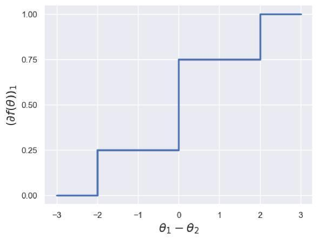
when the distribution of is omitted for brevity. We can express by the pdf of the random variable (Equation 102 in the appendix). Since is a smooth function, a single-valued mapping exists (Theorem 26.1 Rockafellar (1970)). However, is not strictly convex, hence a one-to-one mapping does not exist and it can be concluded that is not a minimal representation of the Perturb-Argmax probability. The derivatives of , corresponding to the probabilities of the , are illustrated in Figure 3.
We defer all details to Section 8.5 in the Appendix. ∎
5.2 Discrete perturbations and identifiablity
We next analyze the identifiability of the Perturb-Argmax distribution representation. Since the max function is not always differentiable, the Perturb-Max function (Equation 11) is not always differentiable. However, since the max function is convex, its sub-differential exists. Unfortunately, the function is a multi-valued function, i.e., for some parameters there exist that both are its sub-gradient. Thus, the probability cannot be identified from the parameters when the perturbation is discrete. This property is demonstrated in the following proposition:
Proposition 5.5.
Let and be a vector of discrete random variables that are uniformly distributed: . Then, the Perturb-Argmax probability distribution is not identifiable.
The proof is provided in Appendix 8.4, and it is based on computing the function analytically by taking the expectation w.r.t. . The function , illustrated in Figure 6 in the appendix, is continuous and differentiable almost everywhere. However, in its overlapping segments, the function is not differentiable, i.e., it has a sub-differential which is a set of sub-gradients. To prove that the Perturb-Argmax probability model is unidentifiable, we show that is a multi-valued mapping when . The sub-differential mapping is illustrated in Figure 3.
6 Experiments
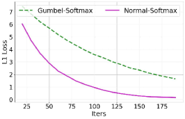
In this section, we demonstrate the advantage of the Gaussian-Softmax over the commonly used Gumbel-Softmax. Experiments in density estimation and variational inference exhibit that, compared to the Gumbel-Softmax, the Gaussian-Softmax enjoys a faster convergence rate and better approximate discrete distributions.
6.1 Approximating discrete distributions
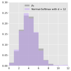
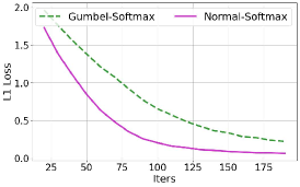
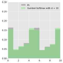
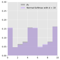
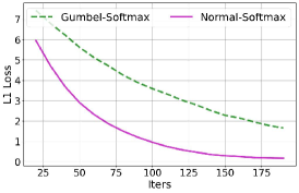
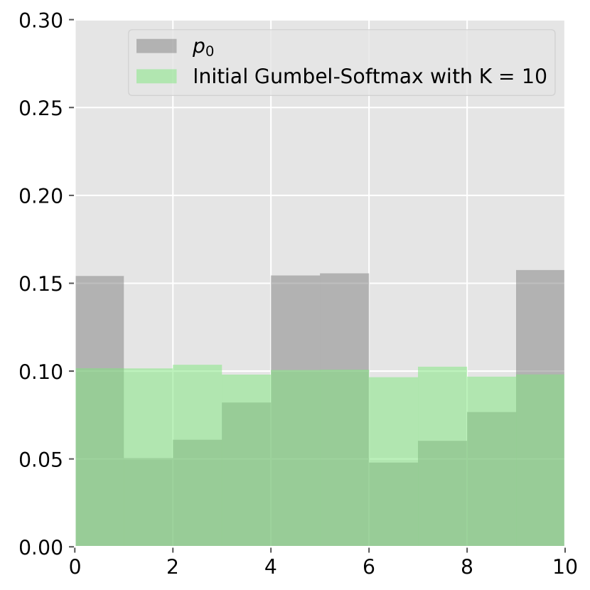
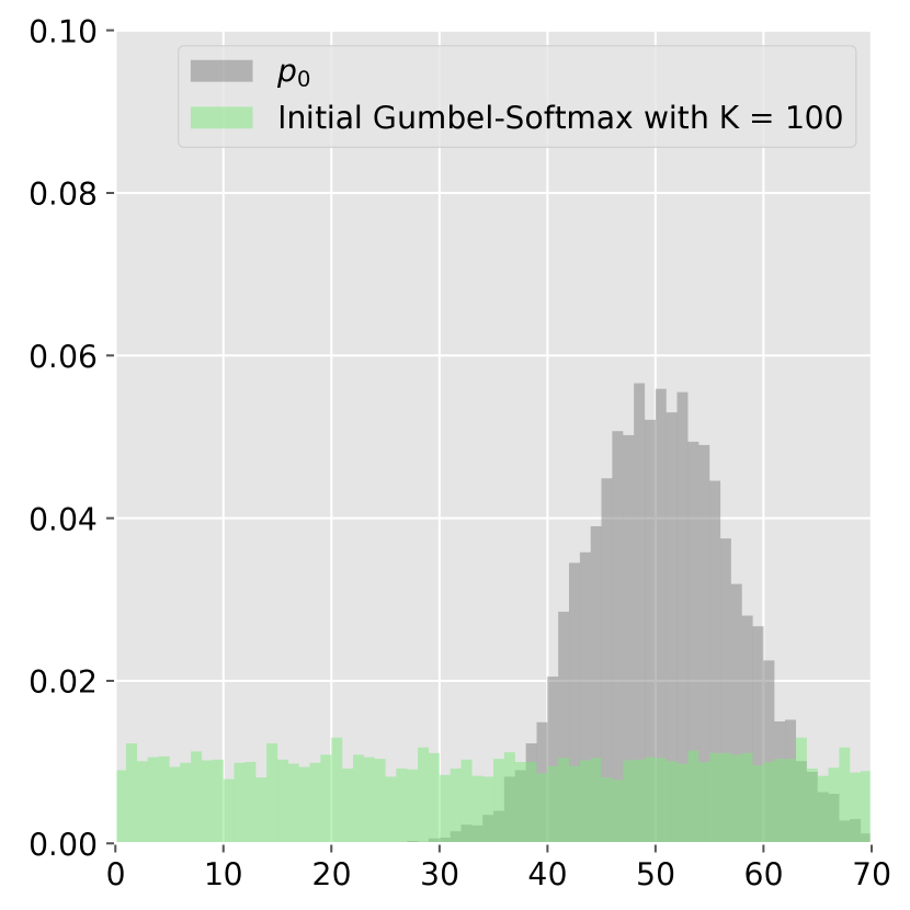
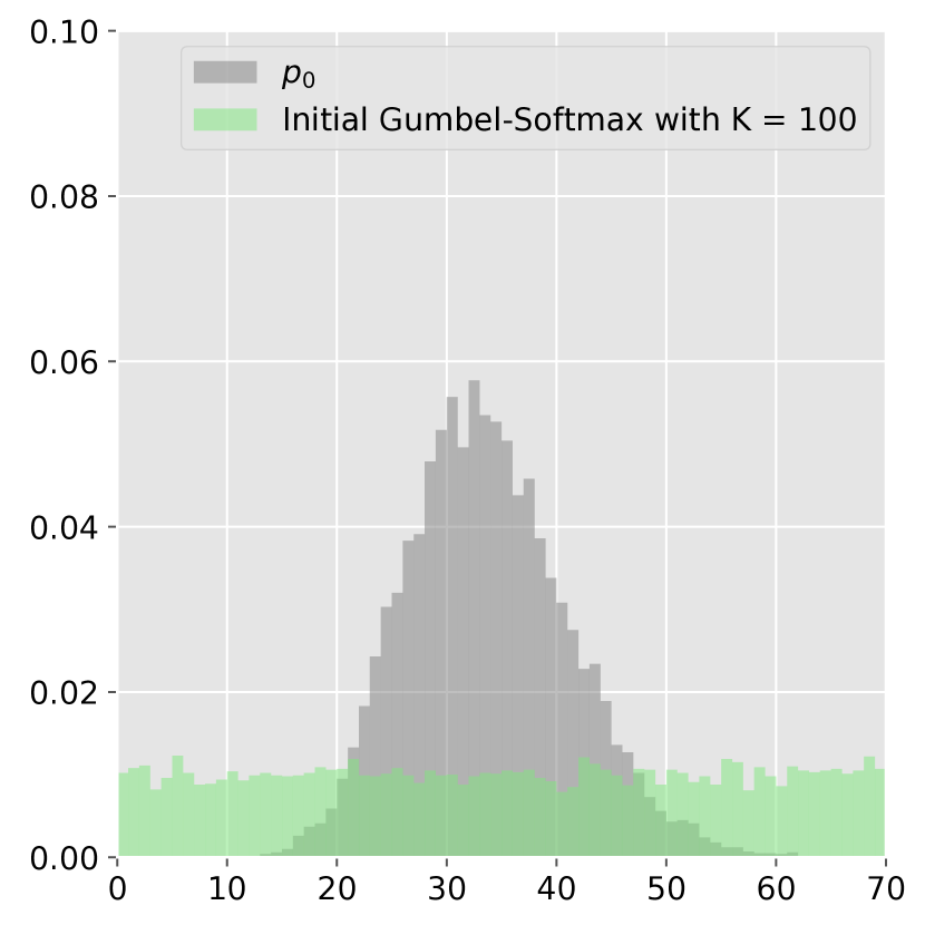
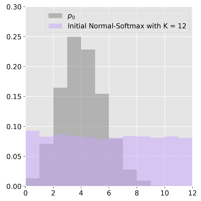
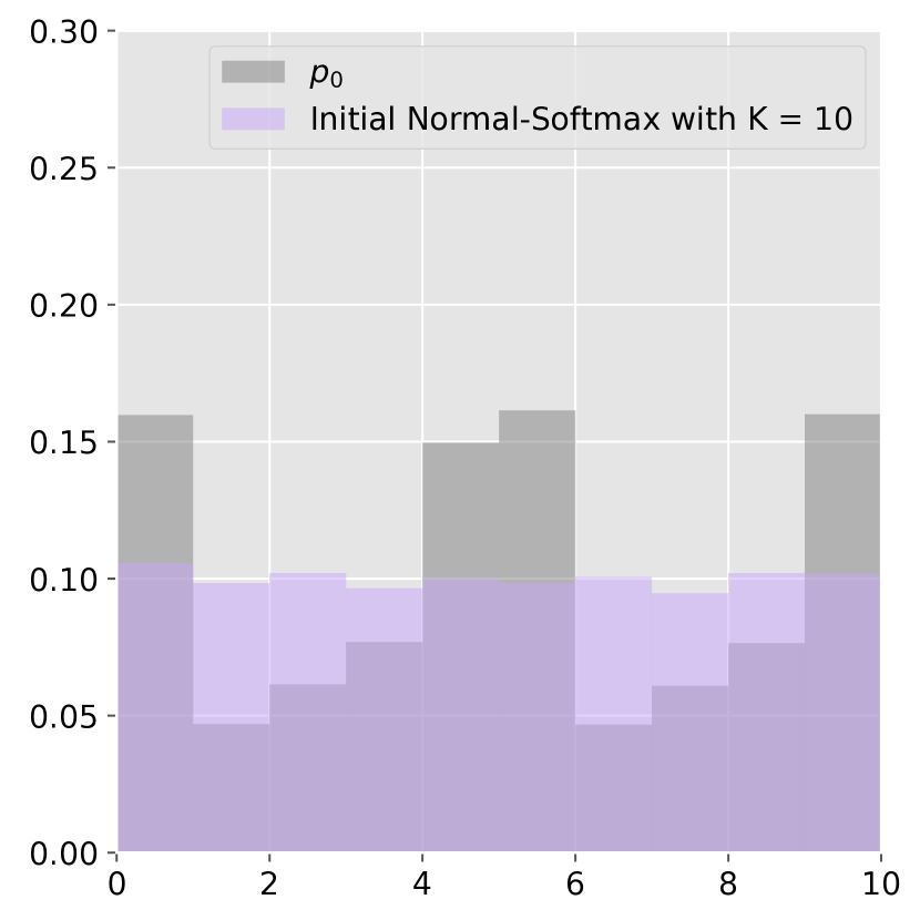
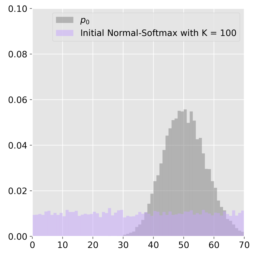
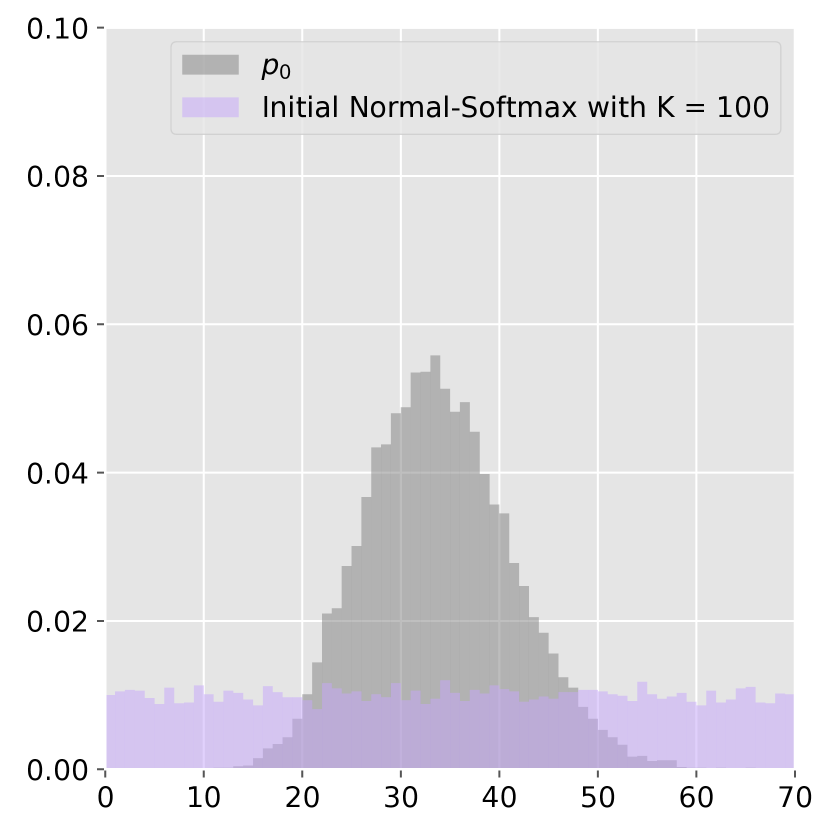
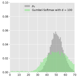
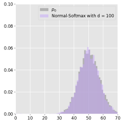
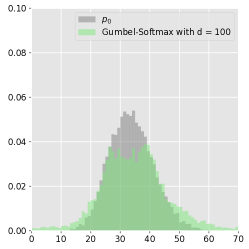
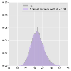
We compare the Gumbel-Softmax and the Normal-Softmax in approximating discrete distributions. The objective function is minimized between the Perturb-Softmax function applied to the fitted parameters of the probability density function and the target discrete distribution, denoted by . We consider two target discrete distributions with finite support: a binomial distribution with parameters , and a discrete distribution with . Figure 4 shows that the Normal-Softmax better approximates both distributions and exhibits faster convergence than the Gaussian-Softmax.
Following the experiment in Potapczynski et al. (2020), we consider discrete distributions with countably infinite support: a Poisson distribution with , and a negative binomial distribution with . Differently from our method, the identifiability of the parameters is lost with the invertible Gaussian parameterization method. Results show that the Normal-Softmax has similar benefits over the Gaussian-Softmax as exhibited for discrete distributions with finite support (Figure 9 in the appendix). Table 1 in the Appendix shows that the approximation based on the Normal-Softmax probability model consistently achieves lower mean and standard deviation . See more details in Appendix 9.1.
6.2 Variational inference
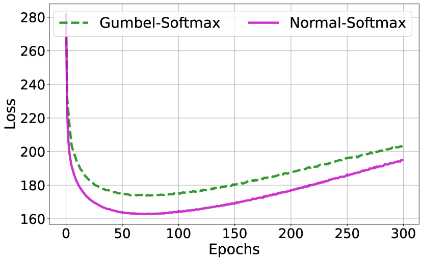
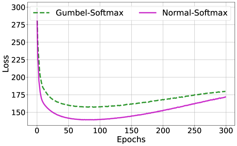
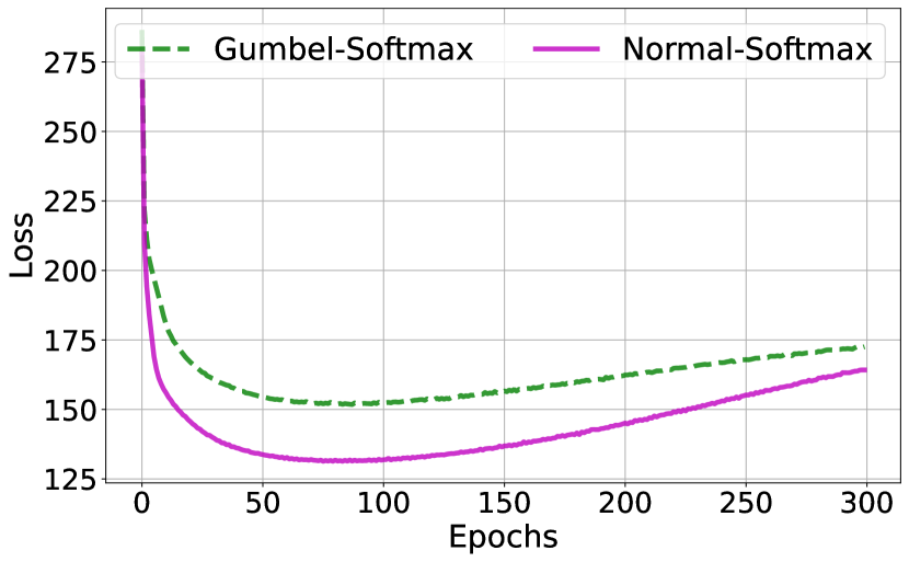
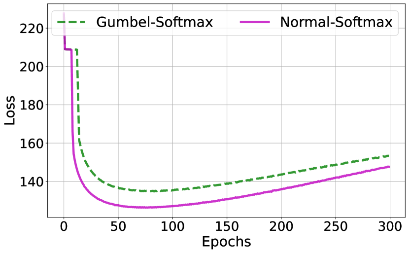
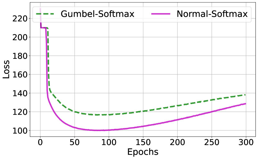
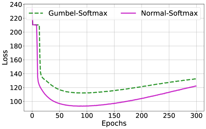
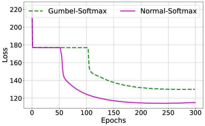
We compared the training ELBO-based loss of categorical Variational-Autoencoders for variables, each is a -dimensional categorical variable, on the binarized MNIST LeCun & Cortes (2005), the Fashion-MNIST (Xiao et al., 2017), and the Omniglot (Lake et al., 2015) datasets for different smooth perturbation distributions. The architecture consists of an encoder of , and matching decoder . We compare the training convergence when propagating gradients with the Normal-Softmax or the Gumbel-Softmax, both performed with a temperature equal to . Results show that the former achieves better and faster learning convergence in all experiments (Figures 5 and 10).


References
- Abernethy et al. (2014) Abernethy, J., Lee, C., Sinha, A., and Tewari, A. Online linear optimization via smoothing. In Conference on learning theory, pp. 807–823. PMLR, 2014.
- Abernethy et al. (2016) Abernethy, J., Lee, C., and Tewari, A. Perturbation techniques in online learning and optimization. Perturbations, Optimization, and Statistics, 233:17, 2016.
- Berthet et al. (2020) Berthet, Q., Blondel, M., Teboul, O., Cuturi, M., Vert, J.-P., and Bach, F. Learning with differentiable perturbed optimizers. In Advances in Neural Information Processing Systems 33 (NeurIPS), pp. 9508–9519, 2020. URL https://proceedings.neurips.cc/paper/2020/file/6bb56208f672af0dd65451f869fedfd9-Paper.pdf.
- Cohen & Hazan (2015) Cohen, A. and Hazan, T. Following the perturbed leader for online structured learning. In Bach, F. and Blei, D. (eds.), Proceedings of the 32nd International Conference on Machine Learning, volume 37 of Proceedings of Machine Learning Research, pp. 1034–1042, Lille, France, 07–09 Jul 2015. PMLR. URL https://proceedings.mlr.press/v37/cohena15.html.
- Cohen Indelman & Hazan (2021) Cohen Indelman, H. and Hazan, T. Learning randomly perturbed structured predictors for direct loss minimization. In Proceedings of the 38th International Conference on Machine Learning, volume 139. PMLR, 2021.
- Geman & Geman (1984) Geman, S. and Geman, D. Stochastic relaxation, gibbs distributions, and the bayesian restoration of images. IEEE Transactions on pattern analysis and machine intelligence, PAMI-6(6):721–741, 1984.
- Goldberg & Jerrum (2007) Goldberg, L. A. and Jerrum, M. The complexity of ferromagnetic ising with local fields. Combinatorics, Probability and Computing, 16(1):43–61, 2007.
- Gumbel (1954) Gumbel, E. J. Statistical theory of extreme values and some practical applications : A series of lectures. 1954. URL https://api.semanticscholar.org/CorpusID:125881359.
- Hannan (1957) Hannan, J. Approximation to bayes risk in repeated play. Contributions to the Theory of Games, 3(2):97–139, 1957.
- Hazan et al. (2010) Hazan, T., Keshet, J., and McAllester, D. Direct loss minimization for structured prediction. In Advances in Neural Information Processing Systems, volume 23, 2010.
- Jang et al. (2017) Jang, E., Gu, S., and Poole, B. Categorical reparameterization with gumbel-softmax. In International Conference on Learning Representations, 2017.
- Kalai & Vempala (2002) Kalai, A. and Vempala, S. Geometric algorithms for online optimization. Journal of Computer and System Sciences, 71(3):291–307, 2002.
- Kalai & Vempala (2005) Kalai, A. and Vempala, S. Efficient algorithms for online decision problems. Journal of Computer and System Sciences, 71(3):291–307, 2005.
- Keshet et al. (2011) Keshet, J., Cheng, C.-C., Stoehr, M., and McAllester, D. A. Direct error rate minimization of hidden markov models. In INTERSPEECH, 2011.
- Kingma & Ba (2017) Kingma, D. P. and Ba, J. Adam: A method for stochastic optimization, 2017.
- Kingma et al. (2014) Kingma, D. P., Rezende, D. J., Mohamed, S., and Welling, M. Semi-supervised learning with deep generative models. In Proceedings of the 27th International Conference on Neural Information Processing Systems - Volume 2, NIPS’14, pp. 3581–3589, Cambridge, MA, USA, 2014. MIT Press.
- Lake et al. (2015) Lake, B. M., Salakhutdinov, R., and Tenenbaum, J. B. Human-level concept learning through probabilistic program induction. Science, 350(6266):1332–1338, 2015. doi: 10.1126/science.aab3050. URL https://www.science.org/doi/abs/10.1126/science.aab3050.
- LeCun & Cortes (2005) LeCun, Y. and Cortes, C. The mnist database of handwritten digits. 2005. URL https://api.semanticscholar.org/CorpusID:60282629.
- Lorberbom et al. (2019) Lorberbom, G., Gane, A., Jaakkola, T., and Hazan, T. Direct optimization through for discrete variational auto-encoder. Advances in neural information processing systems, 32, 2019.
- Luce (1959) Luce, R. D. Individual Choice Behavior: A Theoretical analysis. Wiley, New York, NY, USA, 1959.
- Maddison et al. (2017) Maddison, C. J., Mnih, A., and Teh, Y. W. The concrete distribution: A continuous relaxation of discrete random variables. In International Conference on Learning Representations, 2017.
- Martins & Astudillo (2016) Martins, A. and Astudillo, R. From softmax to sparsemax: A sparse model of attention and multi-label classification. In Proceedings of The 33rd International Conference on Machine Learning, volume 48 of Proceedings of Machine Learning Research, pp. 1614–1623. PMLR, 2016.
- Mnih & Gregor (2014) Mnih, A. and Gregor, K. Neural variational inference and learning in belief networks. In Xing, E. P. and Jebara, T. (eds.), Proceedings of the 31st International Conference on Machine Learning, volume 32 of Proceedings of Machine Learning Research, pp. 1791–1799, Bejing, China, 22–24 Jun 2014. PMLR.
- Niculae et al. (2018) Niculae, V., Martins, A., Blondel, M., and Cardie, C. SparseMAP: Differentiable sparse structured inference. In Dy, J. and Krause, A. (eds.), Proceedings of the 35th International Conference on Machine Learning, volume 80 of Proceedings of Machine Learning Research, pp. 3799–3808. PMLR, 10–15 Jul 2018.
- Pogančić et al. (2020) Pogančić, M. V., Paulus, A., Musil, V., Martius, G., and Rolinek, M. Differentiation of blackbox combinatorial solvers. In International Conference on Learning Representations, 2020.
- Potapczynski et al. (2020) Potapczynski, A., Loaiza-Ganem, G., and Cunningham, J. P. Invertible gaussian reparameterization: Revisiting the gumbel-softmax. In Larochelle, H., Ranzato, M., Hadsell, R., Balcan, M., and Lin, H. (eds.), Advances in Neural Information Processing Systems, volume 33, pp. 12311–12321. Curran Associates, Inc., 2020.
- Rakhlin et al. (2012) Rakhlin, S., Shamir, O., and Sridharan, K. Relax and randomize : From value to algorithms. In Pereira, F., Burges, C., Bottou, L., and Weinberger, K. (eds.), Advances in Neural Information Processing Systems, volume 25. Curran Associates, Inc., 2012. URL https://proceedings.neurips.cc/paper_files/paper/2012/file/53adaf494dc89ef7196d73636eb2451b-Paper.pdf.
- Ramesh et al. (2021) Ramesh, A., Pavlov, M., Goh, G., Gray, S., Voss, C., Radford, A., Chen, M., and Sutskever, I. Zero-shot text-to-image generation. In International conference on machine learning, pp. 8821–8831. Pmlr, 2021.
- Rockafellar (1970) Rockafellar, R. T. Convex analysis. Princeton Mathematical Series. Princeton University Press, Princeton, N. J., 1970.
- Salakhutdinov & Hinton (2009) Salakhutdinov, R. and Hinton, G. Deep boltzmann machines. In van Dyk, D. and Welling, M. (eds.), Proceedings of the Twelth International Conference on Artificial Intelligence and Statistics, volume 5 of Proceedings of Machine Learning Research, pp. 448–455, Hilton Clearwater Beach Resort, Clearwater Beach, Florida USA, 16–18 Apr 2009. PMLR. URL https://proceedings.mlr.press/v5/salakhutdinov09a.html.
- Song et al. (2016) Song, Y., Schwing, A. G., Zemel, R. S., and Urtasun, R. Training deep neural networks via direct loss minimization. In ICML, 2016.
- Wainwright & Jordan (2008) Wainwright, M. and Jordan, M. Graphical models, exponential families, and variational inference. Foundations and Trends in Machine Learning, 1:1–305, 01 2008. doi: 10.1561/2200000001.
- Xiao et al. (2017) Xiao, H., Rasul, K., and Vollgraf, R. Fashion-mnist: a novel image dataset for benchmarking machine learning algorithms, 2017.
7 APPENDIX
7.1 Related work
7.1.1 Convexity
We consider convex functions over its convex domain and follow the notation in Rockafellar (1970). A function over a domain is convex if for every and it holds that . A function is strictly convex if for every and , it holds that . Whenever is twice differentiable, a function is strictly convex if its Hessian is positive definite.
Convexity is a one-dimensional property. A function is convex if and only if its one-dimensional reduction is convex in every admissible direction , i.e., whenever . A twice differentiable function is strictly convex if the second derivative of is positive in every admissible direction . In this case, we denote by and call it a directional derivative:
| (16) |
A multivariate function is differentiable if its directional derivative is the same in every direction , namely for every .
Convexity admits duality correspondence. Any primal convex function has a dual conjugate function
| (17) | |||||
| (18) |
Since is a convex function, its domain is a convex set.
A sub-gradient satisfies for every . The sub-gradient is intimately connected to directional derivatives. Theorem 23.2 in Rockafellar (1970) states that
| (19) |
The vector is admissible if for small enough .
The set of all sub-gradients is called sub-differential at and is denoted by . A convex function is differentiable at when consists of a single vector, and it is denoted by . The sub-differential is a multi-valued mapping between the primal parameters and dual parameters, i.e.,
| (20) |
One can establish with this property the definition of sub-gradient at the optimal point . In this case, , where the sub-gradient is taken with respect to at the maximal argument . From the linearity of the sub-gradient, there holds: , or equivalently, . Using the connection between sub-gradients and directional derivatives, one can show that whenever directional derivatives exist, one can infer a sub-gradient, i.e., the set of all sub-gradients contains the relative interior of , cf. Theorem 23.4 Rockafellar (1970):
| (21) |
7.2 Perturb-Softmax probability distributions
7.2.1 Completeness and minimality of the Softmax operation
Theorem 7.1.
The representation of the softmax distribution defined over is complete. It is minimal when the corresponding log-sum-exp
| (22) |
is a strictly convex function (A paraphrase of Wainwright & Jordan (2008), Proposition 3.1).
Proof.
First, we note that the derivatives of (Eq. 22),
| (23) |
correspond to the softmax probabilities (Eq. 1). is a Gibbs model, hence the representation is complete.
Let and denote , . Then, for
| (24) | |||||
| (25) |
Applying Hölder’s inequality to Equation 25 :
| (26) | ||||
| (27) | ||||
| (28) |
Therefore, it holds that
| (29) |
proving that is convex.
Hölder’s inequality holds with equality if and only if there exists a constant such that
| (30) | |||||
| (31) | |||||
| (32) |
in which case and are linearly constrained and there exists some such that . Therefore, when the representation of is minimal is strictly convex.
Then, consider any , such that . Hölder’s inequality holds strictly as there can not exist a constant such that Equation 32 holds for all if , proving that the representation of is minimal.
Consider . Then, let , and denote and . The proof requires showing that if there exists such that . Equivalently, it requires proving that if it holds that for any , then for all . Explicitly,
| (33) | |||||
| (34) |
Then, by marginalization it holds that
| (35) | |||||
| (36) | |||||
| (37) |
which concludes the proof.
is complete by the conditions of our completeness theorems by setting at the positions and everywhere else.
is complete by the conditions of our completeness theorems by setting at the positions and everywhere else. ∎
Corollary 7.2.
The derivative of the expected log-sum-exp (Equation 6) is a probability function.
Proof.
Denote , then
| (38) | |||||
| (39) |
Also,
| (40) |
∎
7.3 Supporting proof for Theorem 4.1
First, we prove that (Equation 6) is a closed proper convex function and is also essentially smooth. is a convex function as a maximum of convex (linear) functions. Then, is proper as its effective domain is nonempty and it never attains the value , since . is infinitely differentiable throughout the domain, therefore it is a smooth function throughout its domain. is a smooth convex function on , therefore it is in particular essentially smooth. The smoothness of guarantees its continuity, and since can be considered a closed set, then is a closed function.
Given the conditions of the theorem on , we can construct a series for which for every . We prove that approaches the zero-one probability vector as .
| (43) | |||||
The limit argument holds since the probability of decay as they tend to infinity. This proves that the zero-one distributions are limit points of probabilities in , i.e., .
7.4 Proof of Lemma 4.2
In the following, we prove the strict convexity of the expected log-sum-exp of Lemma 4.2.
Proof.
Let and . Then
| (44) |
where and . Applying Hölder’s inequality we obtain the convexity condition of the log-sum-exp function:
| (45) |
To prove strict convexity we note that Hölder’s inequality for non-negative vectors holds with equality if and only if there exists a constant such that for every , or equivalently:
| (46) |
Where . Therefore, if , then for every and consequently it also holds when applying the logarithm function and taking an expectation with respect to . ∎
8 Perturb-Argmax probability distributions
Corollary 8.1.
We prove that the derivative of the expected maximizer is the probability of the . Namely, that .
Proof.
First, by differentiating under the integral:
| (47) |
Writing a subgradient of the max-function using an indicator function (an application of Danskin’s Theorem):
| (48) |
The proof then follows by applying the expectation to both sides of Equation 48. ∎
8.1 Supporting proof for Theorem 5.1
Given the conditions on , we can construct a series for which for every . We show that approaches the zero-one probability vector as .
The limit argument holds since the probability of decay as they tend to infinity.
Corollary 8.2.
The convex conjugate of takes the following values:
| (51) |
where denotes for which .
Proof.
Then, the convex conjugate of , when is denoted by is
| (52) | |||||
| (53) | |||||
| (54) | |||||
| (55) | |||||
| (56) | |||||
| (57) | |||||
| (58) | |||||
| (59) | |||||
| (60) |
where denotes for which .
∎
8.2 Proof of Lemma 5.2
Proof.
By reparameterization
| (61) |
The proof concludes by differentiating under the integral sign while noting that is differentiable. ∎
8.3 Proof of Theorem 5.3
In what follows we prove the minimality of the Perturb-Argmax of Theorem 5.3.
Proof.
Similarly to the Perturb-Softmax setting, we prove that under these conditions the function is strictly convex. For this we rely on its one dimensional function and show that . Since the function is convex then , and it is enough to show that depends on , for which it follows that and consequently .
is the directional derivative in every admissible direction , for . The theorem conditions assert that is not the constant vector, i.e., , where is some constant and is the all-one vector.
We assume, without loss of generality, that is chosen between two indexes, namely . This is possible as we treat to be . We denote by the differentiable probability density function of . We denote remaining random variables as , their probability density function by their measure .
We analyze
is the threshold for which shifts the maximal value to , namely .
With this notation,
| (63) |
Their difference is composed of four terms:
Taking the limit to zero , the last two terms cancel out, since when taking the limit then and by definition, or equivalently, . Therefore
| (64) |
We conclude that by the conditions of the theorem is a function of since there exists for which and the probability density function therefore it assigns mass on the intervals and . Therefore is non-constant function of and . ∎
8.4 Proof of Proposition 5.5
Let , and consider i.i.d. random variables , such that . Let denote the expected perturbed maximum over the domain . Let take values over the extended real domain . Clearly, .
Then, can be explicitly expressed as:
Equation 8.4 suggests that takes the following form:
| (66) |
Recall, that we aim to prove that the Perturb-Argmax probability model is unidentifiable. The function , illustrated in Figure 6 in the appendix, is continuous and differentiable almost everywhere. However, in its overlapping segments, i.e., when , and , the function is not differentiable, i.e., it has a sub-differential which is a set of sub-gradients. To prove that the Perturb-Argmax probability model is unidentifiable, we show that is a multi-valued mapping when . In particular, we show that every probability distribution with satisfies .
For this task, we recall the connection between sub-gradients and directional derivatives: if for every . When , then , thus for the direction for which holds . Recall that if for every . Thus we conclude that must satisfy . Since the same holds to then . Taking both these conditions, when . Therefore, is multi-valued mapping, or equivalently, the parameters are not identifying probability distributions. The sub-differential mapping is
| (67) |
as illustrated in Figure 3.
8.5 Proof of Proposition 5.4
The perturb-max function can be expressed as
| (68) | ||||
| (69) | ||||
| (70) | ||||
| (71) | ||||
| (72) |
when the second equation holds since , and the distribution of is omitted for brevity.
Define and . Then, the random variable has a triangular distribution. The random variable has the following cdf:
| (73) | ||||
| (74) |
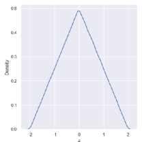
The random variable has the following pdf, also verified in simulation of the density of the difference between 1M iid random variables (Figure 7):
| (75) |
With the pdf of the random variable (Equation 75) consider the appropriate range of .
-
1.
Case:
In this case , therefore
(76) (77) (78) (79) -
2.
Case:
(80) (81) (82) (83) (84) -
3.
Case:
(85) (86) (87) (88) (89) (90) (91) (92) (93) (94) (95) (96) -
4.
Case:
In this case , therefore
(97) (98) (99) (100)
To conclude,
| (101) |
Alternatively, one writes
| (102) |
The derivative of (Equation 101), corresponds to the probabilities of the arg max, :
| (103) |
| (104) |
Then, the partial derivatives and sum to , as expected.
| (105) |
-
1.
Case:
(106) (107) The global minimum of the derivative w.r.t. , for , since
(108) in which case . The global maximum of the derivative w.r.t. , for , in which case .
The global maximum of the derivative w.r.t. , for , since
(109) in which case . The global minimum of the derivative w.r.t. , for , in which case .
9 Experiments
We use a GB 6-Core Intel Core i7 CPU in both experiments.
9.1 Approximating discrete distributions
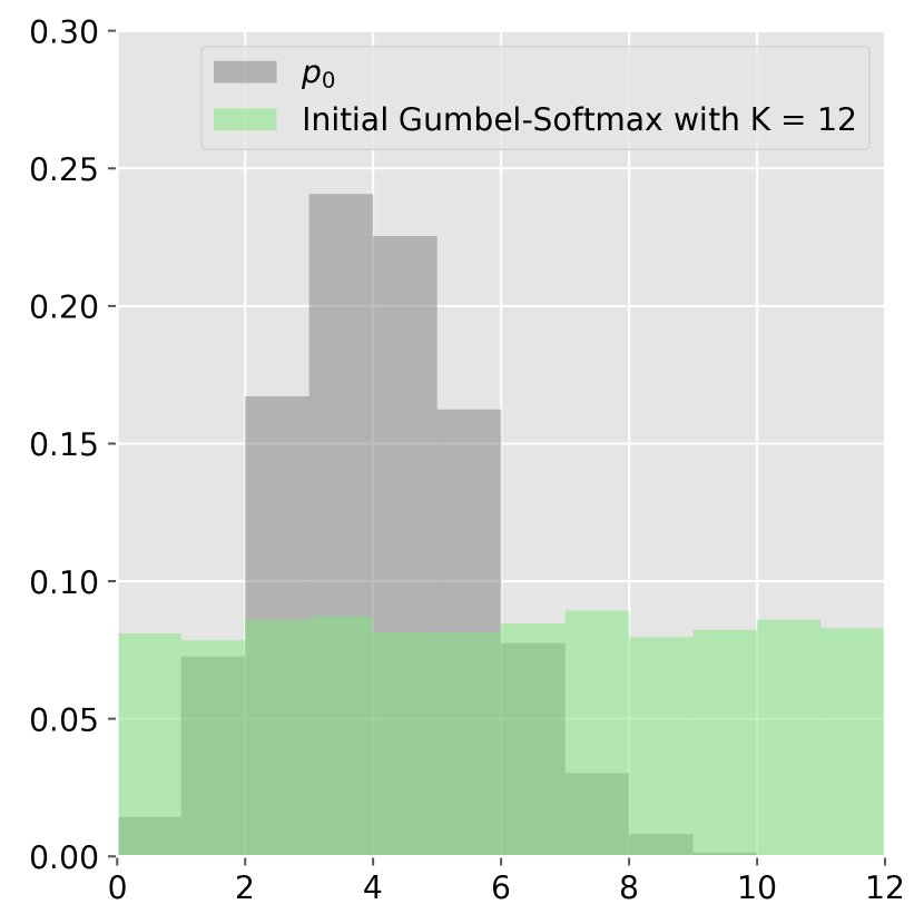
Our experiments are based on the publicly available code of Potapczynski et al. (2020). In all experiments, a thousand samples from a target distribution are sampled to approximate its probability density function parameters, based on the objective function. Optimization is based on the Adam optimizer (Kingma & Ba, 2017) with a learning rate . The fitted parameters are initialized uniformly, as visualized in Figure 8. Figure 9 shows results for fitting discrete distributions with countably infinite support: a Poisson distribution with , and a negative binomial distribution with respectively. The Normal-Softmax distribution better approximates both distributions and exhibits faster convergence than the Gaussian-Softmax.
Table 1 shows the average and standard deviation objective between the approximated probability density function and the four target discrete distributions of both models after iterations, computed over the dimension of the fitted models. The approximation based on the Normal-Softmax probability model achieves lower mean and standard deviation in all cases.
| Target Distribution | Normal-Softmax | Gumbel-Softmax |
|---|---|---|
| Discrete | 0.026 0.002 | 0.0270.002 |
| Binomial | 0.0360.003 | 0.177 0.014 |
| Poisson | 0.0900.001 | 0.618 0.007 |
| Negative Binomial | 0.083 0.001 | 0.417 0.004 |

9.2 Variational inference
This experiment is based on the publicly available implementation of the Gumbel-Softmax-based implementation of the discrete VAE in Direct-VAE. Optimization is based on the Adam optimizer (Kingma & Ba, 2017) with a learning rate of . Batch size is set to . We use the regular train/ test splits and follow previous research splits (e.g., as in Lorberbom et al. (2019)). The MNIST and the Fashion-MNIST datasets’ training set comprises images, and the test set comprises images. For the Omniglot, the training set comprises images, and the test set comprises images.
Figure 10 shows the results of the variational inference experiment for the Fashion-MNIST dataset (Xiao et al., 2017) with discrete variables, each is a -dimensional categorical variable, .