Normal Modes of Rouse-Ham Symmetric Star Polymer Model
Abstract
The Rouse-Ham model is a simple yet useful dynamics model for an unentangled branched polymer. In this work, we study the normal modes of the Rouse-Ham type coarse-grained symmetric star polymer model. We model a star polymer by connecting multiple arm beads to a center bead by harmonic springs. In the Rouse-Ham model, the dynamics of the bead positions can be decomposed into the normal modes, which are chosen to be orthogonal to each other. Due to the existence of degenerate eigenvalues, the eigenmodes do not directly correspond to the normal modes. We propose several methods to construct the normal modes for the coarse-grained symmetric star polymer model. We show that we can construct the normal modes by using a simple permutation or the Hadamard matrix. These methods give symple and highly symmetric orthogonal modes, but work just for a special number of arms. We also show that we can construct the normal modes by using the discrete Fourier transform (DFT) matrix. This method is applicable for an arbitrary number of arms.
1 INTRODUCTION
Coarse-grained simple dynamics models are sometimes quite useful to study various dynamical and rheological behaviors of polymeric materials. One simple yet useful model is the Rouse model[1, 2], in which a linear polymer chain is modeled by connecting beads by linear springs. Beads do not interact each other except via the harmonic spring potentials, and they obey the Langevin equation with a constant friction coefficient. The Rouse model can be generalized to polymers with more complex architectures such as star polymers and comb polymers. Ham[3] developed such a generalized model and how the chain architecture affects the linear viscoelasticity.
The Rouse-Ham model is a standard model to analyze the dynamics of an unentangled branched polymer. For example, the viscoelastic and dielectric relaxation behaviors of unentangled star chains can be well described by the Rouse-Ham model[4]. Even for entangled polymers, some long-time dynamical behaviors can be well described by the Rouse-Ham model governed by the constraint release (CR) mechanism[5, 6]. (Strictly speaking, the CR-based Rouse model is different from the Rouse model based on the Langevin equation. At the long-time scale, nonetheless, they exhibit almost the same relaxation behavior.[7]) Recently, Zhang and coworkers[8, 9] utilized the Rouse-Ham model to study nonlinear rheological behaviors of an end-associative tetra-arm star polymer solution.
We have one difficulty when we utilize the Rouse-Ham model to analyse star polymer dynamics. If the star polymer is symmetric (if all the arms have the same molecular weight), some eigenmodes of the Rouse-Ham model are degenerate. This is in contrast to the Rouse model for a linear chain, where all the eigenmodes are not degenerate. If we are interested only on linear viscoelasticity, this degeneracy is not serious. We need only the eigenvalue distribution to calculate the linear viscoelasticity. However, if we want to study the chain dynamics explicitly, care is required. This is because the degenerate eigenmodes are not orthogonal in general. We will be required to construct orthogonal normal modes by combining non-orthogonal eigenmodes.
In this work, we consider how to construct orthogonal normal modes for the Rouse-Ham type symmetric star polymer model. We propose three different methods to systematically construct orthogonal eigenmodes. The first method is based on the permutation of one specific eigenvector. This method works only for a tetra-arm star polymer. The second method is based on the Hadamard matrix[10]. This works for other numbers of arms, but the applicability is still limited. The third method is based on the discrete Fourier transform (DFT) matrix[11, 12]. Unlike other two methods, this works for any number of arms. After we show the construction methods, we briefly discuss some possible applications of proposed methods.
2 MODEL
We model a symmetric star polymer with -arms by beads connected by harmonic springs. We assume that . We describe the position of the -th bead as (). One bead () represents the branch point, and other beads () represent free ends of arms. We may call the zeroth bead as the center bead and other beads as the arm beads. The coarse-grained effective interaction energy is
| (1) |
Here, is the Boltzmann coefficient, is the temperature, and is the equilibrium root mean square arm size. In the Rouse-Ham model, the beads obey the (overdamped) Langevin equation with a constant friction:
| (2) |
where is the friction coefficient and is the Gaussian white noise. The noise satisfies the fluctuation-dissipation relation: , ( represents the statistical average and is the unit tensor). The Brownian force (which has the dimension of the force) which appear in the underdamped Langevin equation corresponds to . By substituting eq (1) into eq (2), we have
| (3) |
where is the element of the matrix defined as
| (4) |
In what follows, we call as the Rouse-Ham matrix. In this work, we use bold sans-serif letters to express vectors and matrices for the bead indices, in order to distinguish them from the vectors and matrices in the three dimensional space.
Eq (3) is linear in . Therefore, it is convenient to introduce the normal modes. With the normal modes, eq (3) can be rewritten as a set of independent Langevin equations. The normal modes can be constructed by orthogonalizing the Rouse-Ham matrix , in the same way as the Rouse model for a linear chain[1, 2]. To construct normal modes, we calculate the eigenmodes of . We express the -th eigenvector and eigenvalue as (which is an -dimensional column vector) and (). The eigenvector and eigenvalue satisfy . Then the -th eigenmode of eq (3) is calculated as . The relaxation time of the -th eigenmode is if . If all the eigenvectors are orthogonal, the thus constructed eigenmodes become the orthogonal normal modes. However, if the Rouse-Ham matrix has degenerate eigenvalues, the eigenvectors for degenerate eigenvalues are not orthogonal in general. In such a case, cannot be employed as the normal modes unless they are properly orthogonalized.
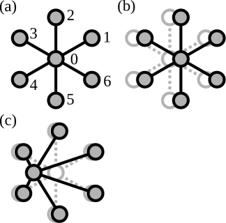
The eigenvalues and eigenvectors of given by eq (4) can be calculated rather easily, if we do not care about the orthogonality. The Rouse model for a linear chain has the zeroth mode with the zero eigenvalue, which corresponds to the center of mass motion. In the same way, we have the zeroth eigenvector and eigenvalue as (the superscript “T” represents the transpose) and . Then eq (3) has the zeroth normal mode as the center of mass position:
| (5) |
The remaining eigenvalues are non-zero. The eigenvalues for are degenerate: . The -th eigenvector and eigenvalue are and . The -th normal mode is given as
| (6) |
Fig. 1 shows images for the translation and deformation by the zeroth and -th normal modes, respectively.
Since the eigenmodes for are degenerate, the explicit forms of eigenvectors () are not that clear. Ham[3] showed that so-called the span vectors correspond to the eigenmodes. The -th span vector can be constructed as (). Unfortunately, Ham’s span vectors are not orthogonal, and thus we cannot employ the Ham span vectors as normal modes. The -th element of the -th eigenvector , which corresponds to the -th span vector, becomes
| (7) |
The zeroth element is always zero. Thus it would be convenient to express and use the -dimensional vector instead of for . It would be intuitive to show as an matrix:
| (8) |
These eigenvectors are clearly not orthogonal because . In what follows, we simply call as the -th span vector, since it can be directly related to the Ham span vector as .
In the case where only the eigenvalue distribution is important, the existence of orthogonal eigenvectors is sufficient. We do not need their explicit forms. For example, to calculate the linear viscoelasticity, we do not need the explicit expression of the normal modes. However, if we want to know the dynamics of bead positions, we will be required to construct orthogonal normal modes. In principle, we can construct orthogonal eigenvectors starting from non-orthogonal yet linearly independent eigenvectors, by using such as the Gram-Schmidt orthogonalization[13] and introduction of some small perturbations. But if we naively apply the Gram-Schmidt orthogonalization to , the resulting eigenvectors become very complicated (especially when is large). Handling of perturbations is also very complicated. In Sec. 3, we show that we can construct orthogonal eigenvectors in three different methods without such complicated processes.
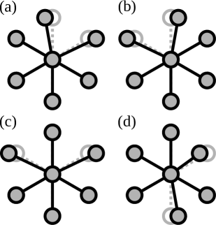
Before we proceed to the construction of normal modes, we show some properties of the span vectors . If we add two span vectors and , we have
| (9) |
Eq (9) corresponds to an eigenvector with the eigenvalue , too, and thus it can be used as a new span vector. By comparing eqs (7) and (9), we find that the position of in is “shifted” from to . This is physically natural, because a symmetric star polymer is symmetric under the exchange of two arms. In a similar way, we can “shift” positions of and several times. Then the general form of the span vector is
| (10) |
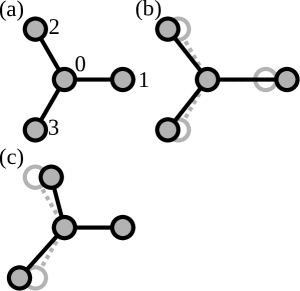
for , , and . Fig. 2 shows some span vectors.
3 RESULTS
3.1 Permutation approach
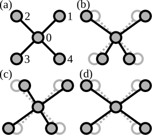
We consider the case where is even. We collect general span vectors, of which non-zero elements are not overlapped each other. Then we can construct an eigenvector , of which element can take only or . Without loss of generality, we can fix the first element: . Then we can construct other eigenvectors as follows, by considering permutations. We select elements from and set them . We set the remaining elements to be . The number of the eigenvectors constructed in this way is . On the other hand, we should have only orthogonal eigenvectors. Therefore, the following condition for should be satisfied: . For , this condition is satisfied only for . Therefore, we limit ourselves to the case of .
We have the following permutation-based eigenvectors:
| (11) |
It is straightforward to show that these eigenvectors are orthogonal: . Then we can construct the normal modes as
| (12) |
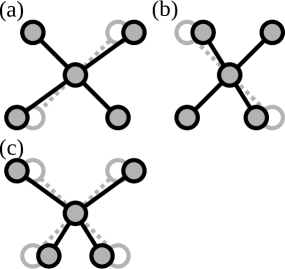
We show images of deformations by orthogonal normal modes by eqs (11) and (12) in Fig. 3.
3.2 Hadamard matrix approach
The permutation approach in Sec. 3.1 is simple but not applicable for . If we can successfully select eigenvectors which are orthogonal to each other from candidates, we will be able to construct the orthogonal eigenvectors for (of course, should be even). Fortunately, for some , there exists such a set of eigenvectors. We can utilize the Hadamard matrix[10].
The Hadamard matrix is an matrix of which elements consist only of and . Any two columns (or rows) of are orthogonal. One column consists only of (or ). The remaining () columns can be used as the orthogonal eigenvectors, . For convenience, we introduce a dummy vector . Then the eigenvectors are given by the following simple form:
| (13) |
Unfortunately, the Hadamard matrix exists only for some limited (). Thus we cannot utilize this construction method for , for example. We show the explicit forms of the Hadamard matrices for and :
| (14) |
| (15) |
The Hadamard matrices can be numerically constructed by some programs. (“hadamard” function in Octave constructs and returns the Hadamard matrix[14]. Eqs (14) and (15) are calculated by Octave 5.2.0.) The eigenvectors constructed from are the same as eq (11) (). The normal modes can be constructed in the same way as eq (12):
| (16) |
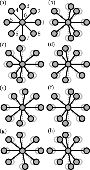
Fig. 4 shows the deformations by the orthogonal normal modes for an octa-arm star polymer () by eq (15) and (16).
For , we can construct different normal modes by exchanging the bead indices for the arm beads. The dynamics of beads is independent of the choice of the normal modes, and thus any physical quantities such as the stress tensor are also independent of the choise.
3.3 DFT matrix approach
Even if we employ the approach based on the Hadamard matrix explained in Sec. 3.2, still we cannot construct the orthogonal eigenvectors in many cases. For example, we cannot construct the eigenvectors for and . Here we consider another method which is applicable for any , based on the discrete Fourier transform (DFT) matrix[11, 12].
We express the -th orthogonal eigenvector to be constructed as . The result of Sec. 3.2 implies that the introduction of a dummy vector which consists only of is useful. Thus we introduce it again, , and construct an matrix by collecting eigenvectors: . Also, we introduce a dummy span vector , and construct an matrix as . Its explicit form is
| (17) |
The dummy span vector is not linearly independent of other span vectors. Actually, it can be expressed in terms of other span vectors:
| (18) |
We consider the eigenvectors of . can be interpreted as the difference operator for a one dimensional periodic system. We introduce a field on a one dimensional periodic lattice with period as . From the periodic condition, we have and thus . We express this field as an -dimensional vector . If we multiply to , we have the difference vector:
| (19) |
This means that can be interpreted as a discrete analog of the differential operator in a continuum one dimensional periodic system. For a continuum one dimensional periodic system, the eigenmodes of are the Fourier modes. Even if the system is discrete, the Fourier modes still work as the eigenmodes.
Therefore, the discrete Fourier modes can be utilized as the orthogonal eigenmodes. We have the -th eigenvector as with being the primitive -th root of unity. becomes the DFT matrix:
| (20) |
It is straightforward to show that is the eigenvector of and it satisfies . (The columns of a DFT matrix are eigenvectors of a cirulant matrix[12].) For , can be constructed as a linear combination of :
| (21) |
where we utilized eq (18). It is also straightforward to show the orthogonality: where represents the Hermitian conjugate vector of . Thus we find that can be utilized as the orthogonal eigenvectors. The normal modes can be constructed by eq (16) with replaced by .
Here, it should be noted that is a complex vector. It can be decomposed into the real and imaginary parts. One may suspect that there are more than eigenvectors if we decompose complex vectors into real vectors. We show that there are just real eigenvectors. The complex conjugate of becomes
| (22) |
Here, represents the complex conjugate vector of , and we utilized the properties of the -th primitive root: and . If is odd, we have and ( and represent the real and imaginary parts, respectively) for . This means that two real eigenvectors constructed from are exactly the same as those from . Therefore, we can construct just real eigenvectors from . If is even, we have for . Then we can construct real eigenvectors. For , we have
| (23) |
where we used . Thus has only the real part (), and we can construct just one real eigenvector from . In total, we can construct real eigenvectors from . Therefore, for any , we have just real eigenvectors.
We show some examples below. For , the DFT matrix becomes
| (24) |
The orthogonal real eigenvectors are constructed as
| (25) |
is essentially the same as the span vector: . For , the DFT matrix is given as
| (26) |
and we have the following orthogonal real eigenvectors:
| (27) |
and are span vectors, again. Figs. 5 and 6 show the deformations by the orthogonal eigenmodes for tri- and tetra-arm star polymers.
The eigenvectors by eq (27) do not coincide to the permutation-based eigenvectors given by eq (11). This is not surprising, because there are many different sets of orthogonal basis vectors. Two sets of orthogonal eigenvectors can be related to each other as
| (28) | ||||
| (29) | ||||
| (30) |
We can employ both eq (11) and (27) to construct normal modes.
In a similar way to the normal modes by the Hadamard matrix, different normal modes can constructed by exchanging the bead indices for the arm beads. As before, the physical quantities are independent of the choise of the indices and normal modes.
4 DISCUSSIONS
4.1 Tetra-arm star chain model with two friction coefficients
Zhang and coworkers proposed a simple Rouse-Ham type tetra-arm star chain model as a coarse-grained model for an end-associative star polymer solution[8, 9]. The chain ends of polymers form transient cross-links, and a traisient network which exhibits viscoelasticity is formed. Zhang et al modeled the dynamics of an end-associative star polymer by tuning the friction coefficient. In their model, the center bead has much smaller friction coefficient than the arm beads. As a result, the center bead is equilibrated almost immediately, and we have the effective dynamic equations only in terms of the arm beads. In this subsection, we consider their model. We introduce the friction coefficient
| (31) |
() and employ the following Langevin equation instead of eq (2):
| (32) |
The fluctuation-dissipation relation is and . We can rewrite eq (32) into the same form as eq (3). Then we have the following Rouse-Ham matrix for this model:
| (33) |
The Rouse-Ham matrix by eq (33) is not symmetric, unlike that by eq (4). We need the left eigenvectors of , which correspond to the transpose of the right eigenvectors of . Therefore, we calculate the right eigenvectors of in what follows.
The zeroth eigenvalue and eigenvector of are and . This gives the following zeroth normal mode:
| (34) |
(If , eq 34 reduces to eq (5). But in this case, and thus , which corresponds to the center of mass position of arm beads.) The fourth eigenvalue and eigenvector of are and . This gives the following fourth normal mode:
| (35) |
Interestingly, the remaining degenerate eigenmodes are exactly the same as those for the model with the common friction coefficient: and ( and ) with
| (36) |
Zhang et al[8, 9] used three span vectors defined as
| (37) |
to analyze the dynamics. They constructed the dynamic equations for and explained nonlinear rheological behavior of an end-associative star chain solution. Although their analyses based on the span vectors seem to be reasonable, in general, orthogonal normal modes are preferred than non-orthogonal span vectors. According to our results in Sec. 3, we can construct the normal modes in a simple and highly symmetric form for . From eqs (11) and (12), we have
| (38) | ||||
| (39) | ||||
| (40) |
We expect that model in Refs. [8] and [9] would be reformulated in a mathematically clearer way with the normal modes given by eqs (34), (35), and (38)-(40). (It should be noted that and the fourth normal mode relaxes quite rapidly, compared with the first, second, and third normal modes. Thus it may be ignored in practice, and we can simply assume that is always fully equilibrated, as in Ref. [8].)
4.2 Gaussian chain model
In Sec. 2, we employed a highly coarse-grained star polymer model. To study the relaxation behavior of individual arms, our model is too coarse-grained. Gaussian-chain-based models would be preferred in some cases. Here we consider a model in which the ends of Gaussian chains are chemically connected to a branch point[4, 6]. It would be possible to formulate the Rouse-Ham matrix for a star Gaussian chain, but the direct calculations would be complicated. Instead of direct construction of the Rouse-Ham matrix, we utilize some properties of eigenmodes for such a symmetric star Gaussian chain. The zeroth mode is the same as the coarse-grained model. It simply represents the center of mass position.
Higher order eigenmodes can be categorized into two types[4]. One is so-called the odd mode, where two arms move in an antisymmetric manner. Another is so-called the even mode, where all the arms move in a symmetric manner. In both cases, the deformation of a single arm is essentially expressed as the eigenmode of a linear Gaussian chain (the Rouse mode). Odd modes are degenerate, and there are eigenmodes which have the same eigenvalue. On the other hand, even modes are not degenerate. If we concentrate only on the degenerate odd-modes, and interpret “a Rouse mode for an arm” as “an arm bead” in our coarse-grained model, the Gaussian chain model reduces to our coarse-grained model. Then we can construct the orthogonal normal modes in the same way as in Sec. 3.
5 CONCLUSIONS
We considered how to construct orthogonal normal modes for the degenerate eigenmodes of the Rouse-Ham type symmetric star chain model. We showed that we can construct normal modes by combining Ham’s span vectors. For , the permutation-based approach gives simple and symmetric normal modes. This approach is applicable only for . For , the columns of the Hadamard matrix can be used to construct the normal modes. The Hadamard matrix exists only for some limited orders, and thus this method cannot be used if the Hadamard matrix of order does not exist. As a construction method for an arbitrary , we showed the construction based on the DFT matrix. The span vectors can be interpreted as the difference operator in one dimensional periodic system, and the columns of the DFT can be used to construct the normal modes. We expect that the results of this work can be utilized to analyze various dynamics models based on the Rouse-Ham model.
ACKNOWLEDGMENT
This work was supported by Grant-in-Aid (KAKENHI) for Scientific Research Grant B No. JP23H01142.
References
- [1] Rouse PE, J Chem Phys, 21, 1272 (1953).
- [2] Doi M, Edwards SF, “The Theory of Polymer Dynamics”, (1986), Oxford University Press, Oxford.
- [3] Ham JS, J Chem Phys, 26, 625 (1957).
- [4] Watanabe H, Yoshida H, Kotaka T, Polym J, 22, 153 (1990).
- [5] Watanabe H, Prog Polym Sci, 24, 1253 (1999).
- [6] Watanabe H, Matsumiya Y, Inoue T, Macromolecules, 35, 2339 (2002).
- [7] Uneyama T, Nihon Reoroji Gakkaishi, 52, 27 (2024).
- [8] Zhang Y, Tang J, Chen Q, Kwon Y, Matsumiya Y, Watanabe H, Nihon Reoroji Gakkaishi, 52, 123 (2024).
- [9] Zhang Y, Tang J, Chen Q, Kwon Y, Matsumiya Y, Watanabe H, Nihon Reoroji Gakkaishi, 52, 143 (2024).
- [10] Zwillinger D (Ed), “CRC Standard Mathematical Tables and Formulae”, 31st ed, (2003), CRC Press, Boca Raton.
- [11] Rao KR, Yip PC (Eds), “The Transform and Data Compression Handbook”, (2001), CRC Press, Boca Raton.
- [12] Grady LJ, Polimeni JR, “Discrete Calculus: Applied Analysis on Graphs for Computational Science”, (2010), Springer, London.
- [13] Gautschi W, “Numerical Analysis”, 2nd ed, (2012), Springer, New York.
- [14] Eaton JW, Bateman D, Hauberg S, Wehbring R, “GNU Octave version 5.2.0 manual: a high-level interactive language for numerical computations” (2020).