Analysis and Simulation of a Coupled Fluid-Heat System in a Thin, Rough Layer

Abstract

We investigate the effective coupling between heat and fluid dynamics within a thin fluid layer in contact with a solid structure via a rough surface. Moreover, the opposing vertical surfaces of the thin layer are in relative motion. This setup is particularly relevant to grinding processes, where cooling lubricants interact with the rough surface of a rotating grinding wheel. The resulting model is non-linearly coupled through $(i)$ temperature-dependent viscosity and $(ii)$ convective heat transport. The underlying geometry is highly heterogeneous due to the thin, rough surface characterized by a small parameter $\epsilon>0$ representing both the height of the layer and the periodicity of the roughness.

We analyze this non-linear system for existence, uniqueness, and energy estimates and study the limit behavior $\varepsilon\to 0$ within the framework of two-scale convergence in thin domains. In this limit, we derive an effective interface model in 3D (a line in 2D) for the heat and fluid interactions inside the fluid. We implement the system numerically and validate the limit problem through direct comparison with the $\varepsilon$-model. Additionally, we investigate the influence of the temperature-dependent viscosity and various geometrical configurations via simulation experiments. The corresponding numerical code is freely available on GitHub.

Keywords: Homogenization, mathematical modeling, dimension reduction, two-scale convergence, thin fluid films, numerical simulations

MSC 2020: 35B27, 76-10, 76M50, 65N30, 80M40, 80A19

1 Introduction

This research is motivated by grinding processes, which typically involve three main components: the grinding wheel, the workpiece, and a cooling lubricant. Here, the workpiece is the material being processed or shaped through grinding and the cooling lubricant is a fluid used to reduce friction and heat generation during the grinding process [27]. The grinding wheel itself is usually a composite material consisting of abrasive grains (e.g., diamonds) and a cementing matrix called bond. Given the complex granular surface of the grinding wheel, thin gaps and channels emerge in the contact area of wheel and workpiece allowing the coolant to flow through. Understanding the formation and the influence of these microstructures is crucial in optimizing the usage of coolants [37, 38]. Naturally, resolving the granular wheel structure and the potentially rough workpiece surface is numerically not feasible, creating a need for homogenized models accounting for microscopic effects in an effective way.

Macroscopic models describing the heat dynamics in the grinding gap via an interface temperature field can be found in the literature; see [26] and the references therein. These models are heuristically derived, and microstructures and fluid flow in the gap are not accounted for. Additionally, fluid pressure estimates are also sometimes investigated and used as a tool to control the supply of the coolant fluid [40, 30]. The fluid dynamics in the gap are heavily influenced by the viscosity of the coolant, which in reality is temperature-dependent [32, 33]; and given the large temperature variations during the grinding process this effect should not be ignored as it can influence the quality of the results [15, 39].

Starting with an idealized periodic setup with a small parameter $\varepsilon\ll 1$ characterizing both the length scale of the periodicity as well as the average thickness of the grinding gap, we rigorously derive an effective, homogenized model accounting for the non-linear coupling between heat and fluid flow dynamics in such a grinding setup. This is accomplished by conducting a limiting procedure $\varepsilon\to 0$ within the framework of two-scale homogenization for thin domains.

From a mathematical point of view, homogenization of diffusion problems for thin layers has been extensively studied before with the concept of two-scale convergence; see for example [31, 23]. Effective fluid flow through thin layers was rigorously investigated in [9] and later extended for a periodic roughness in [10]. Starting with the stationary Stokes equation, they proved the validity of the Reynolds equation [34] when the layer height is small when compared to the length of the roughness period. If the periodicity and the height are of the same order (usually called the Stokes roughness regime), a model similar to a Darcy equation is derived. The Reynolds equation plays an important role in lubrication, which has a similar setup to our underlying scenario. The equation has been further studied and homogenized in the literature [11, 20, 5, 14]; see also [28, Section 1] for a great overview. For layers without roughness, the first derivation of the Reynolds equation with the concept of two-scale convergence was achieved in [29]. Flow through a thin layer, without oscillations, coupled with a temperature-dependent viscosity was studied in [4], where a Reynolds equation with temperature-dependent viscosity was rigorously derived. The effective heat transfer between the different components during the grinding process taking into account a potential has recently been studied in [17].

To be more specific, we consider a complex geometry incorporating a rough, thin layer similar to the setup in [10], where the boundaries of the layer additionally are in relative motion to each other (see Fig. 1). In this geometry, we are considering the coupling between a quasi-stationary Stokes system for the fluid flow and the heat dynamics. Here, the strong coupling comes into play via the convection and the temperature-dependence of the viscosity. We show that the resulting non-linear problem has a weak solution (Theorem 1) via a Schauder fixed point argument where uniqueness follows under additional Lipschitz and regularity assumptions (Theorem 2). Utilizing energy estimates, we conduct a limiting procedure $\varepsilon\to 0$ in the framework of two-scale convergence for thin domains and, as our main result, arrive at a homogenized model capturing the effective interplay between heat dynamics and fluid flow (Theorem 3. Please note that the fluid part of this effective model (e.g., when taking the temperature to be constant) is the same as the limit presented in [10, Section 3.3]. Similarly, as for the $\varepsilon$-problem, we are able to establish uniqueness for the homogenized model under additional Lipschitz and regularity assumptions (Theorem 4).

We validate the effective model numerically by directly comparing it with the heterogeneous problem for small choices of $\varepsilon$ in 2D where the computational cost of resolving the rough boundary explicitly is still manageable. Moreover, we conduct several numerical experiments showcasing and investigating the effects of the temperature-dependent viscosity, the roughness pattern, as well as the inflow condition. The code of our implementation is uploaded and made freely accessible on GitHub.

This paper is structured as follows: In Section 2, we start by introducing the geometrical setup, the mathematical model, and the assumptions needed to pass to the limit $\varepsilon\to 0$. In Section 3 the underlying non-linear model is analyzed regarding existence and uniqueness. Additionally, $\varepsilon$-dependent solution estimates are derived. Section 4 demonstrates the homogenization process and in Theorem 3 the effective model is presented. Finally, in Section 5, we investigate and compare the effective model and the resolved micro model with the help of numerical simulations.

2 Underlying geometry, model and assumptions

2.1 Geometry setup

We start by describing the geometry and the assumptions on the regularity of the interface. In the following, the superscript $f$ denotes that a property belongs to the fluid layer, while $s$ denotes objects belonging to the solid bulk atop the fluid layer. The considered time interval is denoted by $S=(0,T)$, for $T>0$.

We consider spatial domains of dimension $d=2,3$. The $i$-th dimensional unit cube will be denoted by $Y^{i}=(0,1)^{i}$. The unit vector are denoted with $e_{i}\in\mathbb{R}^{d}$, for $i=1,\dots,d$. The whole domain $\Omega\subset\mathbb{R}^{d}$, is given by $\Omega=\Sigma\times(0,H)$, with a bounded $d-1$ dimensional cube $\Sigma\subset\mathbb{R}^{d-1}$ with corner coordinates in $\mathbb{Z}^{d-1}$. For the bottom boundary, we will abuse the notation and understand $\Sigma$ both as a set in $\mathbb{R}^{d-1}$ as well as the boundary part $\Sigma\times\{0\}$. Additionally, a point $x\in\Omega$ will also be denoted by $x=(\tilde{x},x_{d})\subset\Sigma\times(0,H)$. With $\Omega_{\varepsilon}=\Sigma\times(0,\varepsilon)$ we denote a thin layer without any roughness.

The rough interface between solid and fluid is given through a $Y^{d-1}$-periodic $C^{1}$ function $\gamma:\overline{Y}^{d-1}\to[\gamma_{0},1]$, with $\gamma_{0}>0$. Here, we choose the lower bound $\gamma_{0}>0$ such that the interface does not touch the bottom boundary, see also Remark 2 for a discussion regarding the case $\gamma_{0}=0$. Additionally, we require that there exists a $\delta>0$ such that $\gamma(\tilde{x})=1$ for all $\tilde{x}$ with $\text{dist}(\tilde{x},\partial Y^{d-1})<\delta$, so the roughness is given by detached humps and does not intersect the outer boundary. This condition is mainly needed for estimating the pressure inside the thin layer; see also Lemma 5.

Since $\tilde{\Omega}$ is a cube with integer corner coordinates, there exists a $\varepsilon_{0}>0$ such that $\tilde{\Omega}$ can be tiled with $\varepsilon_{0}Y^{d-1}$ cells. A finer partitioning can be achieved with $\varepsilon_{n}=\frac{\varepsilon_{0}}{2^{n}}$, where we will suppress the index $n$. For all $\varepsilon<H$ we define the rough solid domain $\Omega^{s}_{\varepsilon}$ and the thin fluid layer $\Omega^{f}_{\varepsilon}$ by

$$\Omega^{s}_{\varepsilon}=\left\{x\in\Omega:x_{d}>\varepsilon\gamma\left(\frac{\tilde{x}}{\varepsilon}\right)\right\}\quad\text{and}\quad\Omega^{f}_{\varepsilon}=\left\{x\in\Omega:0<x_{d}<\varepsilon\gamma\left(\frac{\tilde{x}}{\varepsilon}\right)\right\}.$$

In addition, the interface between the fluid and grinding wheel is given by

$$\Gamma_{\varepsilon}=\left\{x\in\Omega:x_{d}=\varepsilon\gamma\left(\frac{\tilde{x}}{\varepsilon}\right)\right\}.$$

The outer boundary of the grinding wheel will be denoted by $\Sigma^{s}_{\varepsilon}=\partial\Omega^{s}_{\varepsilon}\setminus\Gamma_{\varepsilon}$ and the lateral boundary of the fluid layer by $\Sigma^{f}_{\varepsilon}=\partial\Omega^{f}_{\varepsilon}\setminus(\Sigma\cup\Gamma_{\varepsilon})$. One geometry example is visualized in Fig. 1.

Note, that for the volume and boundary of the fluid layer, it holds $|\Omega^{f}_{\varepsilon}|,|\Sigma^{f}_{\varepsilon}|\in\mathcal{O}(\varepsilon)$ and for the length of the interface and solid boundary $|\Gamma_{\varepsilon}|,|\Sigma^{s}_{\varepsilon}|\in\mathcal{O}(1)$. With $\nu=\nu(x)$ we denote the normal vector pointing outwards on $\partial\Omega$, the normal vectors pointing out of $\Omega^{f}_{\varepsilon}$ are further denoted by $n_{\varepsilon}=n_{\varepsilon}(x)$.

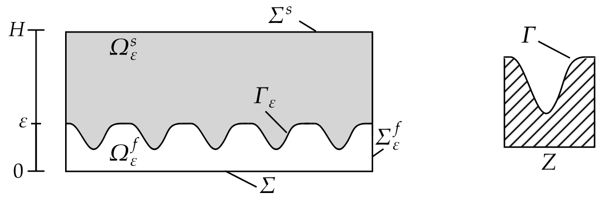
Figure 1: Schematic depiction of the geometric setup. Left: The complete domain with the different subdomains and boundaries. Right: The reference cell.

Regarding our motivating example of a grinding process, the grinding wheel moves over the workpiece, with a given velocity $u_{\text{motion}}$. Since we consider only the section of the grinding gap, it is reasonable to assume that $u_{\text{motion}}\in\mathbb{R}^{d}$ and $u_{\text{motion}}\cdot e_{d}=0$. Because of the movement both domains $\Omega^{s}_{\varepsilon}$ and $\Omega^{f}_{\varepsilon}$ would be time-dependent. To circumvent the homogenization of a moving domain we will view the problem from the reference frame of the grinding wheel and obtain a fixed geometry, see also the model description in the next section.

The outer boundary of the fluid layer is further split into two non-empty sections for fluid in- and outflow. To this end, we split the boundary of $\tilde{\Omega}$ into two parts $\partial\Sigma=\Sigma^{\text{in}}\cup\Sigma^{\text{out}}$. The $\varepsilon$-dependent boundary sections are then given by

$$\Sigma^{\text{in}}_{\varepsilon}=\left\{\left(\tilde{x},\varepsilon\gamma\left(\frac{\tilde{x}}{\varepsilon}\right)\right):\tilde{x}\in\Sigma^{\text{in}}\right\}\quad\text{ and }\quad\Sigma^{\text{out}}_{\varepsilon}=\left\{\left(\tilde{x},\varepsilon\gamma\left(\frac{\tilde{x}}{\varepsilon}\right)\right):\tilde{x}\in\Sigma^{\text{out}}\right\}.$$

Last, we define the reference cell $Z\subseteq Y^{d}$ and reference interface section $\Gamma$ given by

$$Z=\left\{x\in Y^{d}:x_{d}<\gamma(\tilde{x})\right\}\quad\text{ and }\quad\Gamma=\left\{x\in Y^{d}:x_{d}=\gamma(\tilde{x})\right\}.$$

Remark 1.

In the case of grinding, the lower boundary of the fluid layer would also be given by a rough surface describing the workpiece. In our setup, this roughness may be characterized by another function $\gamma_{2}$, but with the same period of $\varepsilon$. It is also reasonable to assume that the workpiece roughness is constant in the direction of $u_{\text{motion}}$, therefore one can again work in a fixed reference frame. To simplify the notation we only consider one oscillating interface, but the following analysis can be transferred to the more general case. The smoothness assumption of $\gamma$ stems from technical reasons and is needed to estimate the fluid pressure.

With the subscript $\tilde{\#}$ we will indicate a space of periodic functions in the directions $1,\dots,d-1$, for example

$$H^{1}_{\tilde{\#}}(Z)\coloneqq\left\{u\in H^{1}_{\text{loc}}(\mathbb{R}^{d}):u_{|Z}\in H^{1}(Z),u(y+e_{i})=u(y)\text{ for almost all }y\in Z\text{ and }i=1,\dots,d-1\right\}.$$

Additionally, we define $\nabla_{\tilde{x}}u=(\partial_{x_{1}}u,\dots,\partial_{x_{d-1}}u,0)$, where a $0$ is appended such that the gradient it compatible with the usual gradient in $\mathbb{R}^{d}$. With $\|\cdot\|_{H^{1}(\Omega^{f}_{\varepsilon}\cup\Omega^{s}_{\varepsilon})}$ we will denote the combined $H^{1}$ norm on both subdomains, e.g.,

$$\|\cdot\|_{H^{1}(\Omega^{f}_{\varepsilon}\cup\Omega^{s}_{\varepsilon})}\coloneqq\sqrt{\|\cdot\|_{H^{1}(\Omega^{f}_{\varepsilon})}^{2}+\|\cdot\|_{H^{1}(\Omega^{s}_{\varepsilon})}^{2}}.$$

2.2 Underlying model equation

For a function $\varphi\in L^{2}(\Omega)$, we use the notation $\varphi_{\varepsilon}^{k}:=\varphi_{|\Omega_{\varepsilon}^{k}}$ for the restriction of $\varphi$ to the subdomain $\Omega_{\varepsilon}^{k}$ for superscript $k=f,s$. A similar notation holds for the coefficients of the models, which are assumed to be constant in each subdomain. We will suppress superscript and the index $\varepsilon$ when possible to improve readability.

We consider a reference frame of the grinding wheel, where instead of a moving interface $\Gamma_{\varepsilon}$ we have a prescribed velocity at the bottom boundary $\Sigma$. To describe the temperature $\theta_{\varepsilon}=(\theta^{s}_{\varepsilon},\theta^{f}_{\varepsilon})$, we utilize heat equations in both domains

$$\partial_{t}\theta_{\varepsilon}-\operatorname{div}\left(\kappa\nabla\theta_{\varepsilon}\right) =0\quad\quad \text{ in }S\times\Omega^{s}_{\varepsilon},$$ (2.1a)

$$\frac{1}{\varepsilon}\partial_{t}\theta_{\varepsilon}-\frac{1}{\varepsilon}\operatorname{div}\left(\kappa\nabla\theta_{\varepsilon}-u_{\varepsilon}\theta_{\varepsilon}\right) =0\quad\quad \text{ in }S\times\Omega^{f}_{\varepsilon},$$ (2.1b)

$$\theta_{\varepsilon}(0,\cdot) =\theta_{\varepsilon,0} \text{ in }\Omega.$$ (2.1c)

Here, $$\kappa=(\kappa^{f}_{\varepsilon},\kappa^{s}_{\varepsilon})$$ describes the heat conductivity in each subdomain.

At the outer boundary, we apply a Dirichlet condition on $\Sigma^{\text{in}}_{\varepsilon}$ for a prescribed cooling temperature (for simplification set to 0, e.g. the temperature is seen relative to the inflow temperature), and on the other boundary sections set the normal derivative to zero,

$$\theta_{\varepsilon} =0 \text{ on }S\times\Sigma^{\text{in}}_{\varepsilon},$$ (2.1d)

$$-\kappa\nabla\theta_{\varepsilon}\cdot\nu =0 \text{ on }S\times\left(\Sigma^{\text{out}}_{\varepsilon}\cup\Sigma^{s}_{\varepsilon}\cup\Sigma\right).$$ (2.1e)

The temperature profiles of the two domains are coupled with a Robin exchange condition

$$-\frac{1}{\varepsilon}\kappa^{f}\nabla\theta^{f}_{\varepsilon}\cdot n_{\varepsilon} =\alpha\llbracket\theta_{\varepsilon}\rrbracket\quad \text{ on }S\times\Gamma_{\varepsilon},$$ (2.1f)

$$-\kappa^{s}\nabla\theta^{s}_{\varepsilon}\cdot n_{\varepsilon} =\alpha\llbracket\theta_{\varepsilon}\rrbracket+f_{\varepsilon}\quad \text{ on }S\times\Gamma_{\varepsilon},$$ (2.1g)

where $\llbracket\theta\rrbracket=(\theta^{f}-\theta^{s})$ denotes the usual jump over a common interface, $\alpha$ denotes the heat exchange parameter and $f_{\varepsilon}$ describes a heat source. Here, the chosen heat source is motivated by our underlying application problem of grinding, there the system heats up through friction between the workpiece and the grinding wheel. Therefore, the heat is produced at the interface. To simplify the notation the heat source is only located on the interface side of the solid domain. Through the Robin condition heat is then also transferred into the fluid.

Next to the temperature, we also model the fluid flow inside $\Omega^{f}_{\varepsilon}$. Fluid velocity $u_{\varepsilon}$ and pressure $p_{\varepsilon}$ are given as the solution of a Stokes equation with temperature-dependent viscosity $\mu$,

$$-\operatorname{div}\left(\mu\left(\theta^{f}_{\varepsilon}\right)\nabla u_{\varepsilon}\right)+\nabla p_{\varepsilon} =0\quad\quad \text{ in }S\times\Omega^{f}_{\varepsilon},$$ (2.1h)

$$\operatorname{div}\left(u_{\varepsilon}\right) =0\quad\quad \text{ in }S\times\Omega^{f}_{\varepsilon},$$ (2.1i)

$$u_{\varepsilon} =u_{\varepsilon,BC} \text{ on }S\times\partial\Omega^{f}_{\varepsilon},$$ (2.1j)

$$\int_{\Omega^{f}_{\varepsilon}}p_{\varepsilon}\,\mathrm{d}x =0 \text{ in }S.$$ (2.1k)

Inertia and buoyancy effects can be assumed neglectable inside the thin layer since usually, fluid movement adjusts itself on a shorter time interval than the temperature. At the outer boundary, we prescribe a velocity $u_{\varepsilon,BC}$ such that

$$u_{\varepsilon,BC}=\begin{cases}0&\text{, if }x\in\Gamma_{\varepsilon},\\ u_{\text{motion}}&\text{, if }x\in\Sigma,\end{cases}$$

and we have inflow at $\Sigma^{\text{in}}_{\varepsilon}$ and outflow at $\Sigma^{\text{out}}_{\varepsilon}$, to be precise

$$\left(u_{\varepsilon,BC}\cdot n_{\varepsilon}\right)_{|\Sigma^{\text{in}}_{\varepsilon}}<0\quad\text{ and }\quad\left(u_{\varepsilon,BC}\cdot n_{\varepsilon}\right)_{|\Sigma^{\text{out}}_{\varepsilon}}\geq 0.$$

Remark 2.

In case of contact between $\Omega^{s}_{\varepsilon}$ and $\Sigma$ (meaning $\gamma_{0}=0$), the temperature model would still be valid, albeit with an additional boundary condition at $\Sigma$. But for dimension $d=2$ the fluid layer would consist of disconnected sections and the model is not reasonable anymore. Even for $d=3$ the boundary conditions for the Stokes equation have to be adapted since there is contact between the moving and non-moving boundary part which influences the analysis of the problem.

2.3 Assumptions on data

To ensure the existence of solutions and be able to pass to the limit $\varepsilon\to 0$ we need multiple assumptions on the data, these are collected in this section.

1. For the coefficients we assume $\alpha,\kappa^{f},\kappa^{s}>0$. Note, that the $\varepsilon$-scaling in (2.1b) is often encountered in the literature [23, 31], to ensure the contributions in the effective model.

2. The temperature dependent viscosity is given by a continuous function $\mu:\mathbb{R}\to\mathbb{R}$ with $\underline{\smash{\mu}}\leq\mu(x)\leq\overline{\mu}$ for some $0<\underline{\smash{\mu}}\leq\overline{\mu}<\infty$.

3. The initial conditions fulfill that $\theta_{\varepsilon,0}\in L^{2}(\Omega)$ and

   $$C_{0}\coloneqq\sup_{\varepsilon>0}{\left(\|\theta_{\varepsilon,0}\|_{L^{2}(\Omega^{s}_{\varepsilon})}+\frac{1}{\sqrt{\varepsilon}}\|\theta_{\varepsilon,0}\|_{L^{2}(\Omega^{f}_{\varepsilon})}\right)}<\infty.$$

4. For the heat source it holds $f_{\varepsilon}\in L^{2}(S\times\Gamma_{\varepsilon})$ and

   $$C_{f}\coloneqq\sup_{\varepsilon>0}\|f_{\varepsilon}\|_{L^{2}(S\times\Gamma_{\varepsilon})}<\infty.$$

5. For the boundary condition of the fluid velocity, we assume there exists a $u_{BC}\in W^{1,\infty}(\partial\Sigma\times(0,1))^{d}$ such that $u_{BC}\cdot e_{d}=0$, $u_{BC}(\tilde{x},0)=u_{\text{motion}}$ and $u_{BC}(\tilde{x},y_{d})=0$ for almost all $\tilde{x}\in\partial\Sigma$ and $y_{d}\geq\gamma_{0}$. The boundary condition on the $\varepsilon$-dependent domain is then defined as $u_{\varepsilon,BC}(x)=u_{BC}(\tilde{x},x_{d}/\varepsilon)$ for $x\in\Sigma^{f}_{\varepsilon}$. To ensure the existence of a solution we also require

   $$\int_{\partial\Omega^{f}_{\varepsilon}}u_{\varepsilon,BC}\cdot n_{\varepsilon}\,\mathrm{d}\sigma_{x}=0.$$ (2.2)

   In addition there has to exists a extension $U_{\varepsilon}\in H^{1}(\Omega^{f}_{\varepsilon})^{d}$ of the boundary function to the inside of $\Omega^{f}_{\varepsilon}$, with $\operatorname{div}{(U_{\varepsilon})}=0$, $U_{\varepsilon}|_{\partial\Omega^{f}_{\varepsilon}}=u_{\varepsilon,BC}$ and $\sqrt{\varepsilon}\|\nabla U_{\varepsilon}\|_{L^{2}(\Omega^{f}_{\varepsilon})}\leq C$, for a $C$ independent of $\varepsilon$.

6. For the initial conditions there are limit functions $\theta^{s}_{0}\in L^{2}(\Omega)$ and $\theta^{f}_{0}\in L^{2}(\Sigma)$ such that $\chi_{\Omega^{s}_{\varepsilon}}\theta_{\varepsilon,0}\to\theta^{s}_{0}$ in $L^{2}(\Omega^{s}_{\varepsilon})$ and $\chi_{\Omega^{f}_{\varepsilon}}\theta^{f}_{\varepsilon,0}\stackrel{{\scriptstyle 2}}{{\rightharpoonup}}\chi_{Z}\theta^{f}_{0}$ in $L^{2}(\Omega_{\varepsilon})$, for $\varepsilon\to 0$. See Section 4 for the definition of two-scale convergence (denoted by $\stackrel{{\scriptstyle 2}}{{\rightharpoonup}}$).

7. For the heat source there is a $f\in L^{2}(S\times\Sigma\times\Gamma)$ such that $f_{\varepsilon}\stackrel{{\scriptstyle 2}}{{\rightharpoonup}}f$, for $\varepsilon\to 0$.

The Assumptions (A1) and (A2) are often encountered in similar problems, especially the properties of $\mu$ are needed to ensure the existence of a solution. That the viscosity depends continuously on the temperature is, for many fluids, physically reasonable [32, Chapter 9.10]. Regarding the continuation in (A5), we can first construct a continuation $U\in H^{1}(\Sigma\times(0,1))$ of $u_{BC}$, with $U(\tilde{x},y)=0$ for $y\geq\gamma_{0}$ [25, Theorem. 3.5]. Setting $U_{\varepsilon}(x)=(U_{1},\dots,\varepsilon U_{d})(\tilde{x},\frac{x_{d}}{\varepsilon})$ gives the desired extension inside the thin layer $\Omega^{f}_{\varepsilon}$, this construction was already derived in [10]. One example that fulfills the above requirements, is a function that varies only in direction $d$, e.g.,

$$u_{\varepsilon,BC}=\begin{cases}\frac{\gamma_{0}-x_{d}/\varepsilon}{\gamma_{0}}u_{\text{motion}}&\text{, if }x_{d}\leq\varepsilon\gamma_{0},\\ 0&\text{, if }x_{d}>\varepsilon\gamma_{0}.\end{cases}$$

We could also utilize a time-dependent boundary function $u_{BC}\in L^{\infty}(S;W^{1,\infty}(\partial\Sigma\times(0,1)))^{d}$, this would not change the following analytical results. To simplify the notation we keep a time-independent $u_{BC}$. The Assumptions (A3), (A4), (A6) and (A7) are, for example, fulfilled by all bounded functions.

3 The microscale model

We start by analyzing the model on the $\varepsilon$-scale to ensure that it is well-posed and to derive solution bounds needed for the limiting procedure. To this end, we first list some technical lemmas needed in the following sections.

3.1 Auxiliary results

Lemma 1 (Extension operator).

For all $\varepsilon>0$, there exist a linear extension operator $\mathbb{E}_{\varepsilon}:H^{1}(\Omega^{f}_{\varepsilon})\to H^{1}(\Omega_{\varepsilon})$ such that

$$\|\mathbb{E}_{\varepsilon}(\psi)\|_{H^{1}(\Omega_{\varepsilon})}\leq C_{\text{ext}}\|\psi\|_{H^{1}(\Omega^{f}_{\varepsilon})},\quad\text{ for all }\psi\in H^{1}(\Omega^{f}_{\varepsilon})$$

and $C_{\text{ext}}<\infty$ can be chosen independent of $\varepsilon$.

Proof.

The extension operators can be constructed by a classical extension procedure [2]. For thin layers, this was carried out in detail, and further studied, in [22, Theorem 1]. ∎

Lemma 2 (Trace estimate).

For $\psi\in H^{1}(\Omega^{f}_{\varepsilon})$ and $\varphi\in H^{1}(\Omega^{s}_{\varepsilon})$ it holds

$$\|\psi\|_{L^{2}(\Gamma_{\varepsilon})}\leq\frac{C^{f}_{\text{tr}}}{\sqrt{\varepsilon}}\|\psi\|_{H^{1}(\Omega^{f}_{\varepsilon})}\quad\text{ and }\quad\|\phi\|_{L^{2}(\Gamma_{\varepsilon})}\leq C^{s}_{\text{tr}}\|\phi\|_{H^{1}(\Omega^{s}_{\varepsilon})},$$

with $C_{\text{tr}}^{f},C_{\text{tr}}^{s}<\infty$ independent of $\varepsilon$.

Proof.

The estimate for $\psi\in H^{1}(\Omega^{f}_{\varepsilon})$ follows by splitting the integral over $\Gamma_{\varepsilon}$ into integrals over the boundary of the cell $\varepsilon Z$, applying a scaling argument followed by a trace estimate in the rescaled domain and then transforming back to the $\varepsilon$ domain.

The estimate for the solid domain $\Omega^{s}_{\varepsilon}$ can be obtained by transforming the domain to a fixed domain without oscillations, as shown in [16, Proposition 2]. ∎

Lemma 3 (Embedding $H^{1}\hookrightarrow L^{4}$).

For all $\varepsilon>0,\psi\in H^{1}(\Omega^{f}_{\varepsilon})$ and $v\in H^{1}_{0}(\Omega^{f}_{\varepsilon})^{d}$ it holds

$$\|\psi\|_{L^{4}(\Omega^{f}_{\varepsilon})}\leq\frac{C_{\text{embed}}^{\theta}}{\varepsilon^{1/4}}\|\psi\|_{H^{1}(\Omega^{f}_{\varepsilon})}\quad\text{and}\quad\|v\|_{L^{4}(\Omega^{f}_{\varepsilon})}\leq C_{\text{embed}}^{u}\|v\|_{H^{1}(\Omega^{f}_{\varepsilon})}$$

for $C_{\text{embed}}^{\theta},C_{\text{embed}}^{u}<\infty$ independent of $\varepsilon$. If in addition $\|v\|_{L^{2}(\Omega^{f}_{\varepsilon})}+\varepsilon\|\nabla v\|_{L^{2}(\Omega^{f}_{\varepsilon})}\leq C\sqrt{\varepsilon}$ then there is a $C<\infty$ independent of $\varepsilon$ such that

$$\|v\|_{L^{4}(\Omega^{f}_{\varepsilon})}\leq\varepsilon^{1/4}C.$$

Proof.

Recall that for space dimension $d=2,3$ the embedding $H^{1}(\Omega)\hookrightarrow L^{4}(\Omega)$ is well defined [18, Chapter 5.6]. For the estimate of $\psi\in H^{1}(\Omega^{\varepsilon}_{\varepsilon})$ we utilize the extension operator $\mathbb{E}$ from Lemma 1. By construction it holds

$$\|\psi\|_{L^{4}(\Omega^{f}_{\varepsilon})}=\|\mathbb{E}_{\varepsilon}(\psi)\|_{L^{4}(\Omega^{f}_{\varepsilon})}\leq\|\mathbb{E}_{\varepsilon}(\psi)\|_{L^{4}(\Omega_{\varepsilon})}.$$

The embedding estimate now follows through integration by substitution to rescale the thin layer $\Omega_{\varepsilon}$ to the domain $\Sigma\times(0,1)$. There we apply an embedding independent of $\varepsilon$ and afterwards transform the integral back to the thin layer.

The first embedding for $v\in H^{1}_{0}(\Omega^{f}_{\varepsilon})^{d}$ is independent of $\varepsilon$ since we can always extend the function by zero to a larger domain, e.g., $\Sigma\times(0,1)$, while preserving the norm. We can again embed independent of $\varepsilon$ on the larger domain. For the last estimate, we use similar arguments as for the first estimate of $\psi$. We extend $v$ by zero to the domain $\Omega_{\varepsilon}$ and use substitution as well as an $\varepsilon$-independent embedding on the rescaled domain $\Sigma\times(0,1)$ to obtain the desired bound

$$\|v\|_{L^{4}(\Omega^{f}_{\varepsilon})}\leq\frac{C}{\varepsilon^{1/4}}\left(\|v\|_{L^{2}(\Omega^{f}_{\varepsilon})}+\varepsilon\|\nabla v\|_{L^{2}(\Omega^{f}_{\varepsilon})}\right)\leq C\varepsilon^{1/4}.$$

∎

3.2 Analysis of the micro model

Next, we investigate the underlying model on the microscale. In the following, $L^{2}_{0}(\Omega^{f}_{\varepsilon})$ denotes all $L^{2}$ functions with zero average, while $H^{1}_{0}(\Omega^{f}_{\varepsilon})$ describes the functions with boundary values equal to 0.

First, we define the spaces in which we seek solutions of the problem. The space for the temperature functions is

$$\Theta_{\varepsilon}=\begin{rcases*}\begin{dcases*}\varphi\in L^{2}(S\times\Omega):\partial_{t}\varphi^{k}\in L^{2}(S;H^{-1}(\Omega^{k})),\varphi^{k}\in L^{2}(S;H^{1}(\Omega^{k}_{\varepsilon}))\text{ for }k=f,s\text{ and }\varphi=0\text{ on }S\times\Sigma^{\text{in}}_{\varepsilon}\end{dcases*}\end{rcases*}.$$

For the fluid velocity and pressure we consider

$$V_{\varepsilon}=\left\{v\in L^{\infty}(S;H^{1}(\Omega^{f}_{\varepsilon})^{d}):v=u_{\varepsilon,BC}\text{ on }\partial\Omega^{f}_{\varepsilon}\text{ and }\operatorname{div}{v}=0\text{ a.e. in }\Omega^{f}_{\varepsilon}\right\}\quad\text{ and }\quad Q_{\varepsilon}=L^{\infty}(S;L^{2}_{0}(\Omega^{f}_{\varepsilon})).$$

The weak formulation of the heat equation, for a fixed $v_{\varepsilon}\in V_{\varepsilon}$, is given by: Find $\theta_{\varepsilon}=(\theta^{s}_{\varepsilon},\theta^{f}_{\varepsilon})\in\Theta_{\varepsilon}$ such that for all $\varphi\in\Theta_{\varepsilon}$ and almost all $t\in S$

$$\begin{split}(\partial_{t}\theta_{\varepsilon},\varphi)_{\Omega^{s}_{\varepsilon}}+(\kappa\nabla\theta_{\varepsilon},\nabla\varphi)_{\Omega^{s}_{\varepsilon}}+\frac{1}{\varepsilon}(\partial_{t}\theta_{\varepsilon},\varphi)_{\Omega^{f}_{\varepsilon}}&+\frac{1}{\varepsilon}(\kappa\nabla\theta_{\varepsilon},\nabla\varphi)_{\Omega^{f}_{\varepsilon}}+\frac{1}{\varepsilon}(v_{\varepsilon}\cdot\nabla\theta_{\varepsilon},\varphi)_{\Omega^{f}_{\varepsilon}}+\alpha(\llbracket\theta_{\varepsilon}\rrbracket,\llbracket\varphi\rrbracket)_{\Gamma_{\varepsilon}}\\ &=(f_{\varepsilon},\varphi^{s})_{\Gamma_{\varepsilon}}.\end{split}$$ (3.1)

Here, $(\cdot,\cdot)_{D}$ denotes the usual $L^{2}$ inner product over the domain $D$. Given a $\psi_{\varepsilon}\in\Theta_{\varepsilon}$, the weak form of the Stokes equation is: Find $(u_{\varepsilon},p_{\varepsilon})\in V_{\varepsilon}\times Q_{\varepsilon}$ such that for all $(v,q)\in H^{1}_{0}(\Omega^{f}_{\varepsilon})^{d}\times L^{2}_{0}(\Omega^{f}_{\varepsilon})$ and almost all $t\in S$

$$\begin{split}&(\mu(\psi_{\varepsilon})\nabla u_{\varepsilon},\nabla v)_{\Omega^{f}_{\varepsilon}}-(p_{\varepsilon},\operatorname{div}{(v)})_{\Omega^{f}_{\varepsilon}}+(q,\operatorname{div}{(u_{\varepsilon})})_{\Omega^{f}_{\varepsilon}}=0.\end{split}$$ (3.2)

Remark 3.

Note that for the solution of Eq. 3.2 it also holds that $\operatorname{div}{(u_{\varepsilon})}=0$ almost everywhere, since by the divergence theorem and Eq. 2.2 we obtain

$$\int_{\Omega^{f}_{\varepsilon}}\operatorname{div}{(u_{\varepsilon})}\,\mathrm{d}x=\int_{\partial\Omega^{f}_{\varepsilon}}u_{\varepsilon}\cdot n_{\varepsilon}\,\mathrm{d}\sigma_{x}=\int_{\partial\Omega^{f}_{\varepsilon}}u_{\varepsilon,BC}\cdot n_{\varepsilon}\,\mathrm{d}\sigma_{x}=0.$$

Therefore, $\operatorname{div}{(u_{\varepsilon})}\in L^{2}_{0}(\Omega^{f}_{\varepsilon})$ and Eq. 3.2 with $v=0$ and $q=\operatorname{div}{(u_{\varepsilon})}$ gives $\|\operatorname{div}{(u_{\varepsilon})}\|_{L^{2}(\Omega^{f}_{\varepsilon})}^{2}=0$.

For a fixed $\varepsilon>0$ we now prove that there exists a solution of the coupled non-linear system given by Eq. 3.1 and (3.2). To show this, we follow a similar strategy as in [8, 33], where we split up the problem, first consider both weak formulations on their own, and then show a solution of the coupled system by a fixpoint argument of an iterative scheme.

Lemma 4.

Let the Assumptions (A1), (A3) and (A4) be fulfilled. For a fixed $\varepsilon>0$ and a given $v_{\varepsilon}\in V_{\varepsilon}$ there exists a unique solution $\theta_{\varepsilon}\in\Theta_{\varepsilon}$ satisfying $\theta_{\varepsilon}(0,\cdot)=\theta_{\varepsilon,0}$ a.e. and Eq. 3.1. In addition, it holds

$$\begin{split}\|\theta_{\varepsilon}\|_{L^{\infty}(S;L^{2}(\Omega^{s}_{\varepsilon}))}+\frac{1}{\sqrt{\varepsilon}}\|\theta_{\varepsilon}\|_{L^{\infty}(S;L^{2}(\Omega^{f}_{\varepsilon}))}+\|\nabla\theta_{\varepsilon}\|_{L^{2}(S;L^{2}(\Omega^{s}_{\varepsilon}))}+\frac{1}{\sqrt{\varepsilon}}\|\nabla\theta_{\varepsilon}\|_{L^{2}(S;L^{2}(\Omega^{f}_{\varepsilon}))}+\|\llbracket\theta_{\varepsilon}\rrbracket\|_{L^{2}(S\times\Gamma_{\varepsilon})}\leq C,\end{split}$$ (3.3)

where $C<\infty$ can be chosen independent of $\varepsilon$ and $v_{\varepsilon}$.

If in addition $\|v_{\varepsilon}\|_{L^{2}(\Omega^{f}_{\varepsilon})}+\varepsilon\|\nabla v_{\varepsilon}\|_{L^{2}(\Omega^{f}_{\varepsilon})}\leq C\sqrt{\varepsilon}$, the time derivative fulfills

$$\begin{split}\|\partial_{t}\theta_{\varepsilon}\|_{L^{2}(S;H^{-1}(\Omega^{s}_{\varepsilon}))}\leq C\quad\text{ and }\quad\|\partial_{t}\theta_{\varepsilon}\|_{L^{2}(S;H^{-1}(\Omega^{f}_{\varepsilon}))}\leq C\sqrt{\varepsilon}.\end{split}$$ (3.4)

Proof.

We start by showing the existence and uniqueness of a solution, for a fixed $v_{\varepsilon}\in V_{\varepsilon}$. First, note that our problem is of the form

$$\langle\partial_{t}\theta_{\varepsilon},\varphi\rangle_{\Omega^{s}_{\varepsilon}}+\frac{1}{\varepsilon}\langle\partial_{t}\theta_{\varepsilon},\varphi\rangle_{\Omega^{f}_{\varepsilon}}+A_{\varepsilon}(\theta_{\varepsilon},\varphi;t)=(f_{\varepsilon},\varphi^{s})_{\Gamma_{\varepsilon}},$$ (3.5)

with the time-dependent bilinear form

$$A_{\varepsilon}(\psi,\varphi;t)\coloneqq(\kappa\nabla\psi,\nabla\varphi)_{\Omega^{s}_{\varepsilon}}+\frac{1}{\varepsilon}(\kappa\nabla\psi,\nabla\varphi)_{\Omega^{f}_{\varepsilon}}+\frac{1}{\varepsilon}(v_{\varepsilon}\cdot\nabla\psi,\varphi)_{\Omega^{f}_{\varepsilon}}+\alpha(\llbracket\psi\rrbracket,\llbracket\varphi\rrbracket)_{\Gamma_{\varepsilon}}.$$

By the embedding $H^{1}(\Omega)\hookrightarrow L^{4}(\Omega)$, the convective term $(v_{\varepsilon}\cdot\nabla\theta_{\varepsilon},\varphi)_{\Omega^{f}_{\varepsilon}}$ is well defined. We obtain that $A_{\varepsilon}$ is bounded, to be precise for all $\psi,\varphi\in\Theta_{\varepsilon}$ and almost all $t\in S$

$$|A_{\varepsilon}(\psi,\varphi;t)|\leq C\left(1+\frac{1}{\varepsilon}+\|v_{\varepsilon}\|_{L^{\infty}(S;H^{1}(\Omega^{f}_{\varepsilon}))}\right)\|\psi(t)\|_{H^{1}(\Omega^{f}_{\varepsilon}\cup\Omega^{s}_{\varepsilon})}\|\phi(t)\|_{H^{1}(\Omega^{f}_{\varepsilon}\cup\Omega^{s}_{\varepsilon})},$$

for a $C<\infty$. Additionally, we have the well-known identity

$$2(v_{\varepsilon}\cdot\nabla\psi,\varphi)_{\Omega^{f}_{\varepsilon}}=(v_{\varepsilon}\cdot\nabla\psi,\varphi)_{\Omega^{f}_{\varepsilon}}-(v_{\varepsilon}\cdot\nabla\varphi,\psi)_{\Omega^{f}_{\varepsilon}}-(\operatorname{div}{(v_{\varepsilon})}\psi,\varphi)_{\Omega^{f}_{\varepsilon}}+(v_{\varepsilon}\cdot n_{\varepsilon},\psi\varphi)_{\partial\Omega^{f}_{\varepsilon}}.$$ (3.6)

Plugging in $\varphi=\psi$, that $\operatorname{div}{(v_{\varepsilon})}=0$ and the boundary conditions on $\partial\Omega^{f}_{\varepsilon}$ into Eq. 3.6 leads to

$$(v_{\varepsilon}\cdot\nabla\psi,\psi)_{\Omega^{f}_{\varepsilon}}=\frac{1}{2}\int_{\Sigma^{\text{out}}_{\varepsilon}}u_{\varepsilon,BC}\cdot n_{\varepsilon}\,\psi^{2}\,\mathrm{d}\sigma_{x}\geq 0$$

for almost all $t\in S$. Therefore, there exists a $\lambda>0$ such that

$$A(\psi,\psi;t)+\lambda\left(\|\psi(t)\|^{2}_{L^{2}(\Omega^{f}_{\varepsilon})}+\|\psi(t)\|^{2}_{L^{2}(\Omega^{s}_{\varepsilon})}\right)\geq C\|\psi(t)\|^{2}_{H^{1}(\Omega^{f}_{\varepsilon}\cup\Omega^{s}_{\varepsilon})}$$

for all $\psi\in\Theta_{\varepsilon}$ and almost all $t\in S$. Given the representation (3.5) and the above estimates for the bilinear form $A$, there exists a unique solution $\theta_{\varepsilon}\in\Theta_{\varepsilon}$ of the problem [36, Chapter 3.2].

For the norm estimate, we utilize the above computations of the convection term, use $\varphi=\theta_{\varepsilon}$ in the weak formulation and integrate afterward over the time interval $(0,t)$, for $t>0$, to obtain

$$\begin{split}\frac{1}{2}\|\theta_{\varepsilon}(t)\|^{2}_{L^{2}(\Omega^{s}_{\varepsilon})}&+\frac{1}{2\varepsilon}\|\theta_{\varepsilon}(t)\|^{2}_{L^{2}(\Omega^{f}_{\varepsilon})}+\|\kappa\nabla\theta_{\varepsilon}\|^{2}_{L^{2}((0,t)\times\Omega^{s}_{\varepsilon})}+\frac{1}{\varepsilon}\|\kappa\nabla\theta_{\varepsilon}\|_{L^{2}((0,t)\times\Omega^{f}_{\varepsilon})}^{2}+\alpha\|\llbracket\theta_{\varepsilon}\rrbracket\|^{2}_{L^{2}((0,t)\times\Gamma_{\varepsilon})}\\ &\leq C_{tr}\|f_{\varepsilon}\|_{L^{2}((0,t)\times\Gamma_{\varepsilon})}\|\theta_{\varepsilon}\|_{L^{2}((0,t);H^{1}(\Omega^{s}_{\varepsilon}))}+\frac{1}{2}\|\theta_{\varepsilon,0}\|^{2}_{L^{2}(\Omega^{s}_{\varepsilon})}+\frac{1}{2\varepsilon}\|\theta_{\varepsilon,0}\|^{2}_{L^{2}(\Omega^{f}_{\varepsilon})},\end{split}$$

with the trace estimate constant $C_{tr}$ on $\Gamma_{\varepsilon}$ from Lemma 2. Applying Young’s inequality followed by Gronwall’s inequality leads to the desired estimate (3.3), where $C$ is independent of $\varepsilon$.

The estimate Eq. 3.4 follows by testing with any $\varphi=(\varphi^{s},\varphi^{f})\in H^{1}(\Omega^{s}_{\varepsilon})\times H^{1}(\Omega^{f}_{\varepsilon})$. One first obtains

$$\begin{split}\bigl{|}\langle\partial_{t}\theta_{\varepsilon},\varphi\rangle_{\Omega^{s}_{\varepsilon}}&+\frac{1}{\varepsilon}\langle\partial_{t}\theta_{\varepsilon},\varphi\rangle_{\Omega^{f}_{\varepsilon}}\bigr{|}\\ &\leq|(\kappa\nabla\theta_{\varepsilon},\nabla\varphi)_{\Omega^{s}_{\varepsilon}}|+\frac{1}{\varepsilon}|(\kappa\nabla\theta_{\varepsilon},\nabla\varphi)_{\Omega^{f}_{\varepsilon}}|+\alpha|(\llbracket\theta_{\varepsilon}\rrbracket,\llbracket\varphi\rrbracket)_{\Gamma_{\varepsilon}}|+|(f_{\varepsilon},\varphi^{s})_{\Gamma_{\varepsilon}}|+|\frac{1}{\varepsilon}(v_{\varepsilon}\cdot\nabla\theta_{\varepsilon},\varphi)_{\Omega^{f}_{\varepsilon}}|\\ &\leq\kappa^{s}\|\nabla\theta_{\varepsilon}\|_{L^{2}(\Omega^{s}_{\varepsilon})}\|\nabla\varphi^{g}\|_{L^{2}(\Omega^{s}_{\varepsilon})}+\frac{\kappa^{f}}{\varepsilon}\|\nabla\theta_{\varepsilon}\|_{L^{2}(\Omega^{f}_{\varepsilon})}\|\nabla\varphi^{f}\|_{L^{2}(\Omega^{f}_{\varepsilon})}+\alpha\|\llbracket\theta_{\varepsilon}\rrbracket\|_{L^{2}(\Gamma_{\varepsilon})}(\|\varphi^{f}\|_{L^{2}(\Gamma_{\varepsilon})}+\|\varphi^{s}\|_{L^{2}(\Gamma_{\varepsilon})})\\ &\hskip 20.0pt+C_{tr}\|f_{\varepsilon}\|_{L^{2}(\Gamma_{\varepsilon})}\|\varphi^{s}\|_{H^{1}(\Omega^{s}_{\varepsilon})}+|\frac{1}{\varepsilon}(v_{\varepsilon}\cdot\nabla\theta_{\varepsilon},\varphi)_{\Omega^{f}_{\varepsilon}}|.\end{split}$$

Choosing $\varphi^{f}=0$, integrating over the time interval $S$, followed by Hölder’s inequality and applying (3.3) gives the desired estimate for $\partial_{t}\theta_{\varepsilon}^{s}$. To estimate $\partial_{t}\theta^{f}_{\varepsilon}$ we can approximate the trace of $\varphi^{s}$ by Lemma 2. The convection term can be estimated with the help of Lemma 3, this leads to

$$\begin{split}|\frac{1}{\varepsilon}(v_{\varepsilon}\cdot\nabla\theta_{\varepsilon},\varphi^{f})_{\Omega^{f}_{\varepsilon}}|\leq\frac{C}{\varepsilon}\|\nabla\theta_{\varepsilon}\|_{L^{2}(\Omega^{f}_{\varepsilon})}\|\varphi^{f}\|_{H^{1}(\Omega^{f}_{\varepsilon})}.\end{split}$$

Setting $\varphi^{s}=0$ and applying the same arguments as before, we obtain the estimate for $\partial_{t}\theta^{f}_{\varepsilon}$. ∎

The additional assumptions on $v_{\varepsilon}$, for the estimate of the time derivative, are no further restrictions since this regularity is obtained naturally.

Lemma 5.

Let the Assumptions (A2) and (A5) be fulfilled. Then for all $\varepsilon>0$ and $\psi_{\varepsilon}\in L^{2}(S;H^{1}(\Omega^{f}_{\varepsilon}))$ there exists a unique solution $(u_{\varepsilon},p_{\varepsilon})\in V_{\varepsilon}\times Q_{\varepsilon}$ of Eq. 3.2. In addition, it holds

$$\frac{1}{\sqrt{\varepsilon}}\|u_{\varepsilon}\|_{L^{\infty}(S;L^{2}(\Omega^{f}_{\varepsilon}))}+\sqrt{\varepsilon}\|\nabla u_{\varepsilon}\|_{L^{\infty}(S;L^{2}(\Omega^{f}_{\varepsilon}))}\leq C\quad\text{ and }\quad\sqrt{\varepsilon}\|p_{\varepsilon}\|_{L^{\infty}(S;L^{2}(\Omega^{f}_{\varepsilon}))}\leq\frac{C}{\varepsilon}$$ (3.7)

for an $C<\infty$ independent of $\varepsilon$ and $\psi_{\varepsilon}$.

Proof.

For almost all $t\in S$, fixed $\psi_{\varepsilon}\in\Theta_{\varepsilon}$ and $\varepsilon>0$ Eq. 3.2 is a standard Stokes problem with varying viscosity. Given our assumptions, there exists a unique solution [25, Theorem 4.1].

For the estimates of the velocity $u_{\varepsilon}$ we test with $v=u_{\varepsilon}-U_{\varepsilon}$ and $q=p_{\varepsilon}$, where $U_{\varepsilon}$ is the extension of the boundary function given by (A5). We obtain for almost all $t\in S$ that

$$\begin{split}\underline{\smash{\mu}}\|\nabla u_{\varepsilon}(t)\|_{L^{2}(\Omega^{f}_{\varepsilon})}^{2}&\leq(\mu(\psi_{\varepsilon}(t))\nabla u_{\varepsilon}(t),\nabla u_{\varepsilon}(t))_{L^{2}(\Omega^{f}_{\varepsilon})}=(\mu(\psi_{\varepsilon}(t))\nabla u_{\varepsilon}(t),\nabla U_{\varepsilon})_{L^{2}(\Omega^{f}_{\varepsilon})}\\ &\leq\overline{\mu}\|\nabla u_{\varepsilon}(t)\|_{L^{2}(\Omega^{f}_{\varepsilon})}\|\nabla U_{\varepsilon}\|_{L^{2}(\Omega^{f}_{\varepsilon})}\leq\overline{\mu}\|\nabla u_{\varepsilon}(t)\|_{L^{2}(\Omega^{f}_{\varepsilon})}\frac{C_{D}}{\sqrt{\varepsilon}}.\end{split}$$

Applying the Poincaré inequality in the thin layer, leads to

$$\|u_{\varepsilon}(t)\|_{L^{2}(\Omega^{f}_{\varepsilon})}\leq C_{p}\|\nabla u_{\varepsilon}(t)\|_{L^{2}(\Omega^{f}_{\varepsilon})},$$

with a Poincaré constant $C_{p}>0$. We can extend the function $u_{\varepsilon}$ by zero to the domain $\Omega_{\varepsilon}=\Sigma\times(0,\varepsilon)$ while preserving the $H^{1}$ norm. The larger layer $\Omega_{\varepsilon}$ is of height $\varepsilon$, there the Poincaré constant can be bounded by $C_{p}\leq\varepsilon C$, with C independent of $\varepsilon$ and we can transfer the constant to the domain $\Omega^{f}_{\varepsilon}$. Therefore, it holds $\|u_{\varepsilon}(t)\|_{L^{2}(\Omega^{f}_{\varepsilon})}\leq\sqrt{\varepsilon}C$ for almost all $t\in S$ and we derived the desired estimates for the velocity field.

The estimate for the pressure is trickier. We point to [10, Section 3.4], where the same Stokes problem for the stationary case and independent of a temperature field was investigated. Since our problem is local in time the results can be transferred. The derivation of the pressure estimate is rather involved and follows by extending the pressure gradient $\nabla p_{\varepsilon}$ to the thin layer $\Omega_{\varepsilon}$ and then using Necas inequality. For this the regularity and assumptions of the interface function $\gamma$ are important. ∎

To handle the coupled non-linear problem, we define the solution operators $\mathbb{T}_{\varepsilon}:V_{\varepsilon}\to L^{2}(S\times\Omega)$ mapping a given velocity to the solution of Eq. 3.1, and the solution operator $\mathbb{F}_{\varepsilon}:L^{2}(S\times\Omega)\to V_{\varepsilon}$ of Eq. 3.2 returning only the velocity field of the Stokes problem. We are looking for a fixed point of the operator

$$\mathbb{S}_{\varepsilon}:L^{2}(S\times\Omega)\to L^{2}(S\times\Omega),\quad\psi_{\varepsilon}\mapsto\mathbb{T}_{\varepsilon}\left(\mathbb{F}_{\varepsilon}(\psi_{\varepsilon})\right),$$ (3.8)

that characterized the temperature field of the non-linear problem. To show the existence of a fixed point, we start by investigating the continuity properties of $\mathbb{T}_{\varepsilon}$ and $\mathbb{F}_{\varepsilon}$.

Lemma 6.

Let the Assumptions (A2) and (A5) be fulfilled. Given a converging sequence $\{\psi_{k}\}_{k\in\mathbb{N}}\subset L^{2}(S\times\Omega)$ with limit $\psi\in L^{2}(S\times\Omega)$ such that $\psi_{k}\xrightarrow[]{k\to\infty}\psi$ in $L^{2}(S\times\Omega)$. For the solution of the Stokes problem Eq. 3.2 it holds

$$\mathbb{F}_{\varepsilon}(\psi_{k})\xrightharpoonup{k\to\infty}\mathbb{F}_{\varepsilon}(\psi)\quad\text{ in }\quad L^{2}(S;H^{1}(\Omega^{f}_{\varepsilon})).$$

Proof.

Under the given Assumptions there exists for each $\psi_{k}$ a unique solution $(u_{k},p_{k})\in V_{\varepsilon}\times Q_{\varepsilon}$ with $\|u_{k}\|_{L^{\infty}(S;H^{1}(\Omega^{f}_{\varepsilon}))}+\|p_{k}\|_{L^{\infty}(S;L^{2}(\Omega^{f}_{\varepsilon})}\leq C_{\varepsilon}$, where $C_{\varepsilon}$ denotes a $\varepsilon$ dependent constant. Given this bound, we can find a $u\in L^{2}(S;H^{1}(\Omega^{f}_{\varepsilon}))$ and a $p\in L^{2}(S\times\Omega^{f}_{\varepsilon})$ such that there is a subsequence of $(u_{k},p_{k})$, still denoted with $k$, that weakly converges:

$$u_{k}\rightharpoonup u\quad\text{in }L^{2}(S;H^{1}(\Omega^{f}_{\varepsilon}))\quad\text{ and }\quad p_{k}\rightharpoonup p\quad\text{in }L^{2}(S;\Omega^{f}_{\varepsilon}).$$

Given the continuity and bounds of $\mu$, it holds $\mu(\psi_{k})\to\mu(\psi)$ in $L^{2}(S\times\Omega)$. Therefore, we obtain the weak convergence

$$\mu(\psi_{k})\nabla u_{k}\rightharpoonup\mu(\psi)\nabla u\quad\text{in }L^{1}(S\times\Omega^{f}_{\varepsilon}).$$

Since the viscosity is in $L^{\infty}(S\times\Omega^{f}_{\varepsilon})$, we have that $\mu(\psi_{k})\nabla u_{k}$ and $\mu(\psi)\nabla u$ are bounded in $L^{2}(S\times\Omega^{f}_{\varepsilon})$. This lets us conclude

$$\mu(\psi_{k})\nabla u_{k}\rightharpoonup\mu(\psi)\nabla u\quad\text{in }L^{2}(S\times\Omega^{f}_{\varepsilon}),$$

for a subsequence. We are now able to pass to the limit in the weak formulation, to obtain

$$0 =\lim_{k\to\infty}\left[(\mu(\psi_{k})\nabla u_{k},\nabla v)_{S\times\Omega^{f}_{\varepsilon}}-(p_{k},\operatorname{div}{(v)})_{S\times\Omega^{f}_{\varepsilon}}+(q,\operatorname{div}{(u_{k})})_{S\times\Omega^{f}_{\varepsilon}}\right]$$

$$=(\mu(\psi)\nabla u,\nabla v)_{S\times\Omega^{f}_{\varepsilon}}-(p,\operatorname{div}{(v)})_{S\times\Omega^{f}_{\varepsilon}}+(q,\operatorname{div}{(u)})_{S\times\Omega^{f}_{\varepsilon}},$$

for all $(v,q)\in H^{1}_{0}(\Omega^{f}_{\varepsilon})\times L^{2}_{0}(\Omega^{f}_{\varepsilon})$. By localization in time, we see that, for almost all $t\in S$, $(u,p)$ is the solution to the Stokes problem (3.2) in $V_{\varepsilon}\times Q_{\varepsilon}$ corresponding to $\psi$. Because the solution is unique, the whole sequence weakly converges to the same limit. ∎

Lemma 7.

Let the Assumptions (A1), (A3), (A4) and (A5) be fulfilled. Given a weakly converging sequence $\{u_{k}\}_{k\in\mathbb{N}}\subset V_{\varepsilon}$ with limit $u\in V_{\varepsilon}$ such that $u_{k}\xrightharpoonup{k\to\infty}u$ in $L^{2}(S;H^{1}(\Omega^{f}_{\varepsilon}))$, it holds

$$\mathbb{T}_{\varepsilon}(u_{k})\xrightarrow[]{k\to\infty}\mathbb{T}_{\varepsilon}(u)\quad\text{ in }\quad L^{2}(S\times\Omega).$$

Proof.

Given the assumptions and that $u_{k}\in V_{\varepsilon}$, we obtain (by Lemma 4) a sequence $\{\theta_{k}\}_{k\in\mathbb{N}}\subset\Theta_{\varepsilon}$ which is bounded in $\Theta_{\varepsilon}$ independent of $u_{k}$. Therefore, we obtain the weak convergence of a subsequence, still denoted with $k$, and a limit $\theta\in\Theta_{\varepsilon}$, such that $\theta_{k}\rightharpoonup\theta$ in $L^{2}(S;H^{1}(\Omega_{\varepsilon}^{f}\cup\Omega_{\varepsilon}^{g}))$ and $\partial_{t}\theta_{k}\rightharpoonup\partial_{t}\theta$ in $L^{2}(S;H^{-1}(\Omega_{\varepsilon}^{f}\cup\Omega_{\varepsilon}^{g}))$.

Note that the embedding $H^{1}(\Omega^{k}_{\varepsilon})\hookrightarrow L^{2}(\Omega^{k}_{\varepsilon})$ is compact and the embedding $L^{2}(\Omega^{k}_{\varepsilon})\hookrightarrow H^{-1}(\Omega^{k}_{\varepsilon})$ is continuous, for $k=f,g$. Therefore, by Aubin-Lions Lemma, we can compactly embed $\Theta_{\varepsilon}$ into $L^{2}(S\times\Omega)$ and obtain $\theta_{k}\to\theta$ in $L^{2}(S\times\Omega)$.

It remains to show that $\theta=\mathbb{T}_{\varepsilon}(u)$. For this, the convection term has to be considered in more detail, so we can pass to the limit in the weak formulation. With integration by parts, we first obtain

$$(u_{k}\cdot\nabla\theta_{k},\varphi)_{S\times\Omega^{f}_{\varepsilon}}=-(u_{k}\theta_{k},\nabla\varphi)_{S\times\Omega^{f}_{\varepsilon}}+(u_{\varepsilon,BC}\cdot n_{\varepsilon}\theta_{k},\varphi)_{S\times\partial\Omega^{f}_{\varepsilon}},$$

for all $\varphi\in L^{2}(S;H^{1}(\Omega^{f}_{\varepsilon}))$. Given the continuity of the trace operator and that by (A5) the boundary velocity is bounded, we can pass to the limit ($k\to\infty$) in the boundary term. For the first term on the right-hand side, we utilize similar arguments as in Lemma 6. By embedding we find

$$\|u_{k}\theta_{k}\|_{L^{2}(S\times\Omega^{f}_{\varepsilon})}\leq C_{\varepsilon}\|u_{k}\|_{L^{\infty}(S;H^{1}(\Omega^{f}_{\varepsilon}))}\|\theta_{k}\|_{L^{2}(S;H^{1}(\Omega^{f}_{\varepsilon}))}\leq C_{\varepsilon},$$

where $C_{\varepsilon}$ is independent of $k$. Similarly, $u\theta$ is bounded in $L^{2}(S\times\Omega^{f}_{\varepsilon})$ as well. This yields the weak convergence $u_{k}\theta_{k}\rightharpoonup u\theta$ in $L^{2}(S\times\Omega^{f}_{\varepsilon})$. This allows us to pass to the limit $k\to\infty$ in the weak formulation and obtain that $\theta$ is the solution corresponding to the velocity field $u$. Again, the solution to the temperature problem is unique, therefore, the whole sequence converges. ∎

Combining the previous two Lemmas we obtain the continuity of the concatenated operator $\mathbb{S}_{\varepsilon}$.

Corollary 1.

The operator $\mathbb{S}_{\varepsilon}$ defined in Eq. 3.8 is continuous from $L^{2}(S\times\Omega)$ to $L^{2}(S\times\Omega)$.

With the continuity, we can now tackle the existence of a fixed point.

Theorem 1 (Existence).

Let the Assumption (A1)-(A5) be fulfilled. Then the operator $\mathbb{S}_{\varepsilon}$ defined in Eq. 3.8 has a fixed point in $\Theta_{\varepsilon}$.

Proof.

We start by observing, that $\Theta_{\varepsilon}\subset L^{2}(S\times\Omega)$ is convex and non-empty. Additionally, by an embedding argument $\Theta_{\varepsilon,\text{bounded}}$ is a relatively compact set in $L^{2}(S\times\Omega)$. Therefore, we can apply Schauder’s fixed point theorem [35] and obtain that there exists at least one fixed point of the operator $\mathbb{S}_{\varepsilon}$ in $\Theta_{\varepsilon,\text{bounded}}$. ∎

The previous theorem ensures, that, under the given assumptions, there exists a weak solution $(\theta_{\varepsilon},u_{\varepsilon},p_{\varepsilon})$ of the problem (2.1) for all $\varepsilon>0$. By construction of the operator $\mathbb{S}_{\varepsilon}$ the fixed point also fulfills the estimates from Lemma 4 and Lemma 5. To ensure the uniqueness, further assumptions on the regularity of the solution are required, as denoted in the following theorem.

Theorem 2 (Uniqueness).

Let Assumptions (A1)–(A5) be satisfied and let $\mu\colon\mathbb{R}\to\mathbb{R}$ be additionally Lipschitz continuous. If there is a solution $(\theta_{\varepsilon},u_{\varepsilon},p_{\varepsilon})\in\Theta_{\varepsilon}\times V_{\varepsilon}\times Q_{\varepsilon}$ such that $\nabla\theta_{\varepsilon}\in L^{\infty}(S;L^{\nicefrac{{3}}{{2}}}(\Omega_{\varepsilon}^{f}))$ and $\nabla u_{\varepsilon}\in L^{\infty}(S;L^{3}(\Omega_{\varepsilon}^{f}))^{d}$. Then, this solution is the unique fixed point of $\mathbb{S}_{\varepsilon}$.

Proof.

Suppose there are two sets of solutions $(\theta_{\varepsilon}^{i},u_{\varepsilon}^{i},p_{\varepsilon}^{i})\in\Theta_{\varepsilon}\times V_{\varepsilon}\times Q_{\varepsilon}$ ($i=1,2$) with their differences denoted by $(\overline{\theta_{\varepsilon}},\overline{u_{\varepsilon}},\overline{p_{\varepsilon}})$. Furthermore, let $(\theta_{\varepsilon}^{1},u_{\varepsilon}^{1})$ satisfy the additional gradient regularity. Using the weak formulations, it holds

$$(\partial_{t}\overline{\theta_{\varepsilon}},\varphi)_{\Omega^{s}_{\varepsilon}}+(\kappa^{s}\nabla\overline{\theta_{\varepsilon}},\nabla\varphi)_{\Omega^{s}_{\varepsilon}}+\frac{1}{\varepsilon}(\partial_{t}\overline{\theta_{\varepsilon}},\varphi)_{\Omega^{f}_{\varepsilon}}+\frac{1}{\varepsilon}(\kappa^{f}\nabla\overline{\theta_{\varepsilon}},\nabla\varphi)_{\Omega^{s}_{\varepsilon}}\\ +\frac{1}{\varepsilon}(\overline{u_{\varepsilon}}\cdot\nabla{\theta_{\varepsilon}}^{1},\varphi)_{\Omega^{f}_{\varepsilon}}+\frac{1}{\varepsilon}(u_{\varepsilon}^{2}\cdot\nabla\overline{\theta_{\varepsilon}},\varphi)_{\Omega^{f}_{\varepsilon}}+\alpha(\llbracket\overline{\theta_{\varepsilon}}\rrbracket,\llbracket\varphi\rrbracket)_{\Gamma_{\varepsilon}}=0,$$

$$\begin{split}&(\mu(\theta_{\varepsilon}^{2})\nabla\overline{u_{\varepsilon}},\nabla v)_{\Omega^{f}_{\varepsilon}}+((\mu(\theta_{\varepsilon}^{2})-\mu(\theta_{\varepsilon}^{1})))\nabla u_{\varepsilon}^{1},\nabla v)_{\Omega^{f}_{\varepsilon}}-(\overline{p_{\varepsilon}},\operatorname{div}{v})_{\Omega^{f}_{\varepsilon}}+(\operatorname{div}{\overline{u_{\varepsilon}}},q)_{\Omega^{f}_{\varepsilon}}=0.\end{split}$$

for all test functions $(\varphi,v,q)\in\Theta_{\varepsilon}\times V_{\varepsilon}\times Q_{\varepsilon}$ and almost all $t\in S$. Now, choosing $(\varphi,v,q)=(\overline{\theta_{\varepsilon}},\overline{u_{\varepsilon}},\overline{p_{\varepsilon}})$ as test functions, we obtain

$$\frac{1}{2}\frac{\operatorname{d}}{\operatorname{d}t}\|\overline{\theta_{\varepsilon}}\|_{L^{2}(\Omega_{\varepsilon}^{s})}^{2}+c_{g}\|\nabla\overline{\theta_{\varepsilon}}\|_{L^{2}(\Omega_{\varepsilon}^{s})}^{2}+\frac{1}{2\varepsilon}\frac{\operatorname{d}}{\operatorname{d}t}\|\overline{\theta_{\varepsilon}}\|_{L^{2}(\Omega_{\varepsilon}^{f})}^{2}+\frac{c_{f}}{\varepsilon}\|\nabla\overline{\theta_{\varepsilon}}\|_{L^{2}(\Omega_{\varepsilon}^{f})}^{2}+\alpha\|\overline{\theta_{\varepsilon}}\|_{L^{2}(\Gamma_{\varepsilon})}^{2}+\frac{1}{\varepsilon}(u_{\varepsilon}^{2}\cdot\nabla\overline{\theta_{\varepsilon}},\overline{\theta_{\varepsilon}})_{\Omega^{f}_{\varepsilon}}\\ \leq-\frac{1}{\varepsilon}(\overline{u_{\varepsilon}}\cdot\nabla\theta_{\varepsilon}^{1},\overline{\theta_{\varepsilon}})_{\Omega^{f}_{\varepsilon}},$$

$$\begin{split}&\underline{\mu}\|\nabla\overline{u_{\varepsilon}}\|_{L^{2}(\Omega_{\varepsilon}^{f})}^{2}\leq((\mu({\theta_{\varepsilon}}^{1})-\mu({\theta_{\varepsilon}}^{2}))\nabla u_{\varepsilon}^{1},\nabla\overline{u_{\varepsilon}})_{\Omega^{f}_{\varepsilon}}.\end{split}$$

Using the Lipschitz property of the viscosity and Hölder’s and the Poincaré inequality, we are led to

$$\|\overline{u_{\varepsilon}}\|_{H^{1}(\Omega_{\varepsilon}^{f})}^{2}\leq C\|\overline{\theta_{\varepsilon}}\|_{L^{6}(\Omega_{\varepsilon}^{f})}^{2}\|\nabla u_{\varepsilon}^{1}\|_{L^{3}(\Omega_{\varepsilon}^{f})}^{2}.$$ (3.9)

For the heat problem, we first note that

$$(u_{\varepsilon}^{2}\cdot\nabla\overline{\theta_{\varepsilon}},\overline{\theta_{\varepsilon}})_{\Omega^{f}_{\varepsilon}}\geq 0$$

via Eq. 3.6 resulting in

$$\frac{\operatorname{d}}{\operatorname{d}t}\|\overline{\theta_{\varepsilon}}\|_{L^{2}(\Omega_{\varepsilon}^{s})}^{2}+\|\nabla\overline{\theta_{\varepsilon}}\|_{L^{2}(\Omega_{\varepsilon}^{s})}^{2}+\frac{\operatorname{d}}{\operatorname{d}t}\|\overline{\theta_{\varepsilon}}\|_{L^{2}(\Omega_{\varepsilon}^{f})}^{2}+\|\nabla\overline{\theta_{\varepsilon}}\|_{L^{2}(\Omega_{\varepsilon}^{f})}^{2}+\|\llbracket\overline{\theta_{\varepsilon}}\rrbracket\|_{L^{2}(\Gamma_{\varepsilon})}^{2}\\ \leq C_{\varepsilon}\|\overline{u_{\varepsilon}}\|_{L^{6}(\Omega_{\varepsilon}^{f})}\|\overline{\theta_{\varepsilon}}\|_{L^{6}(\Omega_{\varepsilon}^{f})}\|\nabla{\theta_{\varepsilon}}^{1}\|_{L^{\nicefrac{{3}}{{2}}}(\Omega_{\varepsilon}^{f})}.$$ (3.10)

Summing Eqs. 3.9 and 3.10 and integrating over time, we get

$$\|\overline{\theta_{\varepsilon}}(t)\|_{L^{2}(\Omega_{\varepsilon}^{s})}^{2}+\|\overline{\theta_{\varepsilon}}(t)\|_{L^{2}(\Omega_{\varepsilon}^{f})}^{2}+\int_{0}^{t}\left(\|\nabla\overline{\theta_{\varepsilon}}\|_{L^{2}(\Omega_{\varepsilon}^{s})}^{2}+\|\nabla\overline{\theta_{\varepsilon}}\|_{L^{2}(\Omega_{\varepsilon}^{f})}^{2}+\|\llbracket\overline{\theta_{\varepsilon}}\rrbracket\|_{L^{2}(\Gamma_{\varepsilon})}^{2}+\|\overline{u_{\varepsilon}}\|_{H^{1}(\Omega_{\varepsilon}^{f})}^{2}\right)\,\mathrm{d}\tau\\ \leq C_{\varepsilon}\int_{0}^{t}\left(\|\overline{u_{\varepsilon}}\|_{L^{6}(\Omega_{\varepsilon}^{f})}\|\overline{\theta_{\varepsilon}}\|_{L^{6}(\Omega_{\varepsilon}^{f})}\|\nabla{\theta_{\varepsilon}}^{1}\|_{L^{\nicefrac{{3}}{{2}}}(\Omega_{\varepsilon}^{f})}+\|\overline{\theta_{\varepsilon}}\|_{L^{6}(\Omega_{\varepsilon}^{f})}^{2}\|\nabla u_{\varepsilon}^{1}\|_{L^{3}(\Omega_{\varepsilon}^{f})}^{2}\right)\,\mathrm{d}\tau.$$

Focusing on the second term on the right-hand side, we have

$$\int_{0}^{t}\|\overline{\theta_{\varepsilon}}\|_{L^{6}(\Omega_{\varepsilon}^{f})}^{2}\|\nabla u_{\varepsilon}^{1}\|_{L^{3}(\Omega_{\varepsilon}^{f})}^{2}\,\mathrm{d}\tau\leq\|\nabla u_{\varepsilon}^{1}\|_{L^{\infty}(S;L^{3}(\Omega_{\varepsilon}^{f}))}^{2}\|\overline{\theta_{\varepsilon}}\|_{L^{2}(S;L^{6}(\Omega_{\varepsilon}^{f}))}^{2}.$$

Using $\nabla u_{\varepsilon}^{1}\in L^{\infty}(S;L^{3}(\Omega_{\varepsilon}^{f}))^{d}$, the Gagliardo-Nierenberg interpolation inequality, and the scaled Young’s inequality, then leads to

$$C_{\varepsilon}\int_{0}^{t}\|\overline{\theta_{\varepsilon}}\|_{L^{6}(\Omega_{\varepsilon}^{f})}^{2}\|\nabla u_{\varepsilon}^{1}\|_{L^{3}(\Omega_{\varepsilon}^{f})}^{2}\,\mathrm{d}\tau\leq\frac{1}{4}\|\nabla\overline{\theta_{\varepsilon}}\|_{L^{2}(S\times\Omega_{\varepsilon}^{f})}^{2}+C_{\varepsilon}\|\overline{\theta_{\varepsilon}}\|_{L^{2}(S\times\Omega_{\varepsilon}^{f})}^{2}.$$

For the first term on the right-hand side, we use $\nabla\theta_{\varepsilon}^{1}\in L^{\infty}(S;L^{\nicefrac{{3}}{{2}}}(\Omega_{\varepsilon}^{f}))$ to estimate

$$\int_{0}^{t}\|\overline{u_{\varepsilon}}\|_{L^{6}(\Omega_{\varepsilon}^{f})}\|\overline{\theta_{\varepsilon}}\|_{L^{6}(\Omega_{\varepsilon}^{f})}\|\nabla{\theta_{\varepsilon}}^{1}\|_{L^{\nicefrac{{3}}{{2}}}(\Omega_{\varepsilon}^{f})}\,\mathrm{d}\tau\leq C_{\varepsilon}\|\overline{u_{\varepsilon}}\|_{L^{2}(S;H^{1}(\Omega_{\varepsilon}^{f}))}\|\overline{\theta_{\varepsilon}}\|_{L^{2}(S;L^{6}(\Omega_{\varepsilon}^{f}))}$$

which (again using Young’s inequality and the Gagliardo-Nierenberg interpolation) gives

$$C_{\varepsilon}\int_{0}^{t}\|\overline{u_{\varepsilon}}\|_{L^{6}(\Omega_{\varepsilon}^{f})}\|\overline{\theta_{\varepsilon}}\|_{L^{6}(\Omega_{\varepsilon}^{f})}\|\nabla{\theta_{\varepsilon}}^{1}\|_{L^{\nicefrac{{3}}{{2}}}(\Omega_{\varepsilon}^{f})}\,\mathrm{d}\tau\leq\frac{1}{2}\|\overline{u_{\varepsilon}}\|_{L^{2}(S;H^{1}(\Omega_{\varepsilon}^{f}))}^{2}+\frac{1}{4}\|\nabla\overline{\theta_{\varepsilon}}\|_{L^{2}(S\times\Omega_{\varepsilon}^{f})}^{2}+C_{\varepsilon}\|\overline{\theta_{\varepsilon}}\|_{L^{2}(S\times\Omega_{\varepsilon}^{f})}^{2}.$$

Putting everything together aund utilizing Gronwalls inequality shows $\overline{u_{\varepsilon}}=0$ and $\overline{\theta_{\varepsilon}}=0$.

∎

Remark 4.

In 2D, these regularity conditions for uniqueness are actually lower due to the different embeddings available for the Gagliardo-Nierenberg inequality: $\nabla\theta_{\varepsilon}\in L^{\infty}(S;L^{1+\delta}(\Omega_{\varepsilon}^{f}))$ and $\nabla u_{\varepsilon}\in L^{\infty}(S;L^{2+\delta}(\Omega_{\varepsilon}^{f}))^{2}$ for any arbitrarily small $\delta$ is sufficient.

4 Homogenization

To pass to the limit $\varepsilon\to 0$ we utilize the concept of two-scale convergence for thin layers first introduced [31, Definition 4.1] and further developed in following articles, see for example [12, 23] and the references therein. We start by introducing the definition, then consider the existence of limit functions, show strong convergence of the temperature field, and then pass to the limit in the weak formulation. Lastly, we analyze the existence and uniqueness of solutions of the effective model.

4.1 Two scale definition and theory and limit existence

Definiton 1 (Two-scale convergence on thin domains).

• A sequence $u_{\varepsilon}\in L^{2}(S\times\Omega_{\varepsilon})$ is said to weakly two-scale converge to a function $u\in L^{2}(S\times\Sigma\times Y^{d})$ (notation $u_{\varepsilon}\stackrel{{\scriptstyle 2}}{{\rightharpoonup}}u$) if

  $$\lim_{\varepsilon\to 0}\frac{1}{\varepsilon}\int_{S}\int_{\Omega_{\varepsilon}}u_{\varepsilon}(t,x)\varphi\left(t,\tilde{x},\frac{x}{\varepsilon}\right)\,\mathrm{d}x\,\mathrm{d}t=\int_{S}\int_{\Sigma}\int_{Y^{d}}u(t,\tilde{x},y)\varphi(t,\tilde{x},y)\,\mathrm{d}y\,\mathrm{d}\tilde{x}\,\mathrm{d}t,$$ (4.1)

  for all $\varphi\in C(\overline{S\times\Sigma};C_{\tilde{\#}}(\overline{Y}^{d}))$. If in addition

  $$\lim_{\varepsilon\to 0}\frac{1}{\sqrt{\varepsilon}}\|u_{\varepsilon}\|_{L^{2}(S\times\Omega_{\varepsilon})}=\|u\|_{L^{2}(S\times\Sigma\times Y^{d})}$$

  then the sequence is said to strongly two-scale converge.

• A sequence $u_{\varepsilon}\in L^{2}(S\times\Gamma_{\varepsilon})$ is said to weakly two-scale converge to a function $u\in L^{2}(S\times\Sigma\times\Gamma)$ if

  $$\lim_{\varepsilon\to 0}\int_{S}\int_{\Gamma_{\varepsilon}}u_{\varepsilon}(t,x)\varphi\left(t,\tilde{x},\frac{x}{\varepsilon}\right)\,\mathrm{d}\sigma_{x}\,\mathrm{d}t=\int_{S}\int_{\Sigma}\int_{\Gamma}u(t,\tilde{x},y)\varphi(t,\tilde{x},y)\,\mathrm{d}\sigma_{y}\,\mathrm{d}\tilde{x}\,\mathrm{d}t,$$ (4.2)

  for all $\varphi\in C(\overline{S\times\Sigma};C_{\tilde{\#}}(\Gamma))$.

Note, that due to the Assumption (A5) it holds for the boundary condition of the velocity

$$\frac{1}{\sqrt{\varepsilon}}\|u_{\varepsilon,BC}\|_{L^{2}(\partial\Sigma\times(0,\varepsilon))}=\|u_{BC}\|_{L^{2}(\partial\Sigma\times(0,1))},$$

as well as

$$\begin{split}\lim_{\varepsilon\to 0}\frac{1}{\varepsilon}\int_{\partial\Sigma\times(0,\varepsilon)}u_{\varepsilon,BC}\varphi\left(\tilde{x},\frac{x}{\varepsilon}\right)\,\mathrm{d}x&=\lim_{\varepsilon\to 0}\int_{\partial\Sigma}\int_{0}^{1}u_{BC}(\tilde{x},y_{d})\varphi\left(\tilde{x},\frac{\tilde{x}}{\varepsilon},y_{d}\right)\,\mathrm{d}y_{d}\,\mathrm{d}\tilde{x}\\ &=\int_{\partial\Sigma}\int_{Y^{d}}u_{BC}(\tilde{x},y_{d})\varphi(\tilde{x},y)\,\mathrm{d}y\,\mathrm{d}\tilde{x},\end{split}$$ (4.3)

for all $\varphi\in C(\partial\Sigma;C_{\tilde{\#}}(\overline{Y}^{d}))$. The two above properties imply the strong two-scale convergence of the boundary function, $u_{\varepsilon,BC}\stackrel{{\scriptstyle 2}}{{\rightharpoonup}}u_{BC}$.

Given the assumptions on the data and the estimate derived in Section 3.2 we obtain the following limit functions.

Proposition 1 (Existence of limit functions).

Under the Assumption (A1)-(A5), it holds for the weak solution $(\theta_{\varepsilon},u_{\varepsilon},p_{\varepsilon})\in\Theta_{\varepsilon}\times V_{\varepsilon}\times Q_{\varepsilon}$ of Eq. 2.1 that there exists a subsequence still denoted by $(\theta_{\varepsilon},u_{\varepsilon},p_{\varepsilon})$ and:

• a $\theta^{s}\in L^{2}(S;H^{1}(\Omega))\cap H^{1}(S;H^{-1}(\Omega))$ with

  $$\chi_{\Omega^{s}_{\varepsilon}}\theta_{\varepsilon}\to\theta^{s}\text{ in }L^{2}(S\times\Omega)\quad\text{ and }\quad\chi_{\Omega^{s}_{\varepsilon}}\nabla\theta_{\varepsilon}\rightharpoonup\nabla\theta^{s}\text{ in }L^{2}(S\times\Omega)^{d},$$

• a $\theta^{f}\in L^{2}(S;H^{1}(\Sigma))\cap H^{1}(S;H^{-1}(\Sigma))$ and a $\theta_{1}^{f}\in L^{2}(S\times\Sigma;H^{1}_{\tilde{\#}}(Y^{d}))$ with

  $$\chi_{\Omega^{f}_{\varepsilon}}\theta^{f}_{\varepsilon}\stackrel{{\scriptstyle 2}}{{\rightharpoonup}}\chi_{Z}\theta^{f}\quad\text{ and }\quad\chi_{\Omega^{f}_{\varepsilon}}\nabla\theta^{f}_{\varepsilon}\stackrel{{\scriptstyle 2}}{{\rightharpoonup}}\chi_{Z}\left(\nabla_{\tilde{x}}\theta^{f}+\nabla_{y}\theta_{1}^{f}\right),$$

• a $u\in L^{2}(S\times\Sigma;H^{1}_{\tilde{\#}}(\overline{Z}))^{d}$ with

  $$\chi_{\Omega^{f}_{\varepsilon}}u_{\varepsilon}\stackrel{{\scriptstyle 2}}{{\rightharpoonup}}\chi_{Z}u\quad\text{ and }\quad\chi_{\Omega^{f}_{\varepsilon}}\varepsilon\nabla u_{\varepsilon}\stackrel{{\scriptstyle 2}}{{\rightharpoonup}}\chi_{Z}\nabla_{y}u.$$

  It holds $\operatorname{div}_{y}{(u(\tilde{x},y))}=0$ and $\operatorname{div}_{\tilde{x}}{\left(\int_{Z}u(\tilde{x},y)\,\mathrm{d}y\right)}=0$ for almost all $(\tilde{x},y)\in\Sigma\times Z$. Moreover, $u$ has, for almost all $(t,x)\in S\times\Sigma$, the boundary values $u(t,\tilde{x},\tilde{y},0)=u_{\text{motion}}$ for $\tilde{y}\in Y^{d-1}$ and $u(t,\tilde{x},y)=0$ for $y\in\Gamma$ almost everywhere.

• a $p\in L^{2}_{0}(S\times\Sigma\times Z)$ that is periodic in $Y^{d-1}$ and

  $$\varepsilon^{2}\chi_{\Omega^{f}_{\varepsilon}}p_{\varepsilon}\stackrel{{\scriptstyle 2}}{{\rightharpoonup}}\chi_{Z}p.$$

Additionally, on the rough interface, it holds

$$\lim_{\varepsilon\to 0}\int_{S}\int_{\Gamma_{\varepsilon}}\alpha(\theta^{s}_{\varepsilon}-\theta^{f}_{\varepsilon})\varphi\,\mathrm{d}\sigma_{x}\,\mathrm{d}t=\int_{S}\int_{\Sigma}\alpha|\Gamma|(\theta^{s}-\theta^{f})\varphi\,\mathrm{d}\tilde{x}\,\mathrm{d}t,$$

for all admissible test functions $\varphi$.

Proof.

The convergence in $i)$ follows by the estimates of Lemma 4. Given that $\Omega^{s}_{\varepsilon}$ is a domain with a rough boundary given by a height function, it can be transformed to the domain $\Omega$ while preserving the $\Theta_{\varepsilon}$ norm [16]. Therefore, the estimates yield the weak convergence of a subsequence $\theta_{\varepsilon}$ in on $\Omega$ in the $\Theta_{\varepsilon}$ norm. By Aubin–Lions Lemma the embedding $\Theta_{\varepsilon}\hookrightarrow L^{2}(S\times\Omega)$ is compact and since $\chi_{\Omega^{s}_{\varepsilon}}\to\chi_{\Omega}$ in $L^{2}(\Omega)$ we obtain the strong convergence of the solution.

The convergence $ii)$-$iv)$ are obtained by the estimates of Lemma 4 and Lemma 5 and usual two-scale convergence properties, see for example [21, Lemma 4]. Since it holds $\operatorname{div}{(u_{\varepsilon})}=0$ for all $\varepsilon>0$ the divergence-properties follow by a standard argument [1, Proposition 1.14]. The last integral identity is also a common equality, see for example [31, 21] for similar setups and the general proof idea. ∎

To pass to the limit in the non-linear terms, we have Assumption (A5) that yields the Dirichlet data converges strongly in the two-scale sense, but strong convergence of the temperature field in the thin layer $\Omega^{f}_{\varepsilon}$ is required as well.

Proposition 2 (Strong convergence in thin layer).

Let the same assumptions as in Theorem 1 be fulfilled, for the sequence of solutions $\theta_{\varepsilon}$ of Eq. 2.1 and the two-scale limit $\theta^{f}\in L^{2}(S;H^{1}(\Sigma))$ from Proposition 1 it holds

$$\lim_{\varepsilon\to 0}\frac{1}{\sqrt{\varepsilon}}\|\theta_{\varepsilon}\|_{L^{2}(S\times\Omega^{f}_{\varepsilon})}=\|\theta^{f}\|_{L^{2}(S\times\Sigma\times Z)}$$

for at least a subsequence of $\theta_{\varepsilon}$.

Proof.

Follows with the extension operators of Lemma 1 and the same arguments as in [22, Proposition 5]. ∎

Given the strong two-scale convergence and the properties of $\mu$ we obtain the following convergence of the viscosity function.

Corollary 2.

Given the Assumptions (A2) it holds $\chi_{\Omega^{f}_{\varepsilon}}\mu(\theta^{f}_{\varepsilon})\stackrel{{\scriptstyle 2}}{{\rightharpoonup}}\chi_{Z}\mu(\theta^{f})$ strongly in $L^{2}(S\times\Omega^{f}_{\varepsilon})$.

4.2 Homogenized equations

Given the previous results concerning the limit behavior of the solution, we can now carry out the homogenization process in the weak formulation of the problem. The general procedure when determining the effective model consists of three steps:

1. Use smooth test functions, compatible with the two-scale concept, in the weak formulation, to pass to the limit $\varepsilon\to 0$.

2. Try to average and decouple the effective systems to simplify the equations and extract cell problems.

3. Apply a density argument to show that the limit also holds for test functions from more general spaces, for example, for functions $\varphi\in L^{2}(S;H^{1}(\Sigma))$.

Most of the steps are standard for our case, therefore we do not explain everything in detail but only comment on the general limit behavior and explain the important aspects more in-depth. We refer to the literature for the detailed procedure. The complete homogenized model is written down at the end of this section in Theorem 3.

Limit procedure for the heat system.

Starting with the temperature limit inside of $\Omega^{s}_{\varepsilon}$. Given the Assumptions (A6) and (A7) for the convergence of the initial condition and heat source, passing to the limit in the weak formulation can be carried out directly. To be exact, we do not require two-scale convergence inside the bulk domain. We point to [16, Section 5] for a similar setup with a rough interface.

Most of the equations for the temperature limit in $\Omega^{f}_{\varepsilon}$ are also quite standard and we point to [31, 23, 12] for similar setups. As usual for these kinds of diffusion problems, one obtains that the limit $\theta^{f}_{1}$ can be represented by

$$\theta^{f}_{1}(t,\tilde{x},y)=\sum_{i=1}^{d-1}\omega_{i}(y)\partial_{x_{i}}\theta^{f}(t,\tilde{x})$$

where $\omega_{i}\in H^{1}_{\tilde{\#}}(Z)$ is the weak solution of

$$\begin{split}\operatorname{div}_{y}{(\nabla_{y}\omega_{i}+e_{i})}&=0\quad\text{ in }Z,\\ (\nabla_{y}\omega_{i}+e_{i})\cdot n&=0\quad\text{ on }\Gamma\cup\{y\in\partial Z:y_{d}=0\}.\end{split}$$ (4.4)

As an example, we demonstrate how the Dirichlet condition for $\theta^{f}$ is obtained. In a similar fashion the boundary values for $u$ on $\partial Z$ follow. We can test with a $\varphi\in C^{\infty}(\overline{S\times\Sigma},C^{\infty}_{\tilde{\#}}(\overline{Z}))^{d}$ such that $\operatorname{div}_{y}{\varphi}=0$ and $\varphi\left(t,\tilde{x},\frac{x}{\varepsilon}\right)\cdot n_{\varepsilon}=0$ on $\partial\Omega^{f}_{\varepsilon}\setminus\Sigma^{\text{in}}_{\varepsilon}$ which yields

$$\frac{1}{\varepsilon}\int_{S}\int_{\Omega^{f}_{\varepsilon}}\theta^{f}_{\varepsilon}(t,x)\operatorname{div}_{\tilde{x}}{\left(\varphi\left(t,\tilde{x},\frac{x}{\varepsilon}\right)\right)}\,\mathrm{d}x\,\mathrm{d}t=-\frac{1}{\varepsilon}\int_{S}\int_{\Omega^{f}_{\varepsilon}}\nabla\theta^{f}_{\varepsilon}(t,x)\cdot\varphi\left(t,\tilde{x},\frac{x}{\varepsilon}\right)\,\mathrm{d}x\,\mathrm{d}t.$$

Passing to the limit on both sides and afterward integrating by parts on the right side, we obtain

$$\int_{S}\int_{\Sigma}\int_{Z}\theta^{f}(t,\tilde{x})\operatorname{div}_{\tilde{x}}{(\varphi(t,\tilde{x},y))}\,\mathrm{d}y\,\mathrm{d}\tilde{x}\,\mathrm{d}t =-\int_{S}\int_{\Sigma}\int_{Z}\left(\nabla_{\tilde{x}}\theta^{f}(t,\tilde{x})+\nabla_{y}\theta^{f}_{1}(t,\tilde{x},y)\right)\cdot\varphi(t,\tilde{x},y)\,\mathrm{d}y\,\mathrm{d}\tilde{x}\,\mathrm{d}t$$

$$=\int_{S}\int_{\Sigma}\int_{Z}\theta^{f}(t,\tilde{x})\operatorname{div}_{\tilde{x}}{(\varphi(t,\tilde{x},y))}\,\mathrm{d}y\,\mathrm{d}\tilde{x}\,\mathrm{d}t$$

$$\hskip 14.22636pt-\int_{S}\int_{\Sigma^{\text{in}}}\theta^{f}(t,\tilde{x})\int_{Z}\varphi(t,\tilde{x},y)\,\mathrm{d}y\cdot n_{\Sigma}\,\mathrm{d}\sigma_{\tilde{x}}\,\mathrm{d}t.$$

Therefore, $\theta^{f}=0$ almost everywhere on $S\times\Sigma^{\text{in}}$.

To pass to the limit in the convection term, Assumption (A5) as well as the strong two-scale convergence of $\theta^{f}_{\varepsilon}\stackrel{{\scriptstyle 2}}{{\rightharpoonup}}\theta^{f}$ (Proposition 2) are required. To obtain the homogenized problem one can test the equation in the layer with a $\varphi_{\varepsilon}=\varphi_{0}(t,\tilde{x})+\varepsilon\varphi_{1}\left(t,\tilde{x},\frac{x}{\varepsilon}\right)$ with $\varphi_{0}\in C^{\infty}(\overline{S\times\Sigma})$ and $\varphi_{1}\in C^{\infty}(\overline{S\times\Sigma},C_{\tilde{\#}}^{\infty}(\overline{Z}))$, $\varphi_{1}(t,\tilde{x},y)=0$ for almost all $(t,\tilde{x},y)\in S\times\Sigma\times\Gamma$. In the case of the convection term, we can integrate by parts to first obtain

$$\lim_{\varepsilon\to 0}\frac{1}{\varepsilon}(u_{\varepsilon}\nabla\theta_{\varepsilon},\varphi_{\varepsilon})_{S\times\Omega^{f}_{\varepsilon}} =\lim_{\varepsilon\to 0}\frac{1}{\varepsilon}\Bigl{[}-(u_{\varepsilon}\theta_{\varepsilon},\nabla_{\tilde{x}}\varphi_{0})_{S\times\Omega^{f}_{\varepsilon}}-\varepsilon(u_{\varepsilon}\theta_{\varepsilon},\nabla_{\tilde{x}}\varphi_{1})_{S\times\Omega^{f}_{\varepsilon}}-(u_{\varepsilon}\theta_{\varepsilon},\nabla_{y}\varphi_{1})_{S\times\Omega^{f}_{\varepsilon}}$$

$$\hskip 42.67912pt+(u_{\varepsilon}\cdot n_{\varepsilon}\theta_{\varepsilon},\varphi_{0})_{S\times\partial\Omega^{f}_{\varepsilon}}+\varepsilon(u_{\varepsilon}\cdot n_{\varepsilon}\theta_{\varepsilon},\varphi_{1})_{\partial\Omega^{f}_{\varepsilon}}\Bigr{]}$$

Utilizing the strong two-scale convergence we can pass to the limit on the right side, which produces

$$\lim_{\varepsilon\to 0}\frac{1}{\varepsilon}(u_{\varepsilon}\nabla\theta_{\varepsilon},\varphi_{\varepsilon})_{S\times\Omega^{f}_{\varepsilon}} =-(u\theta^{f},\nabla_{\tilde{x}}\varphi_{0})_{S\times\Sigma\times Z}-(u\theta^{f},\nabla_{y}\varphi_{1})_{S\times\Sigma\times Z}+(u_{BC}(\tilde{x},y_{d})\cdot n_{\Sigma}\theta^{f},\varphi_{0})_{S\times\partial\Sigma\times Y^{d}}.$$

Integration by parts in the second term on the right-hand side, that $\operatorname{div}_{y}(u\theta^{f})=0$, the periodicity and boundary values of $\varphi_{1}$ yield $(u\theta^{f},\nabla_{y}\varphi_{1})_{S\times\Sigma\times Z}=0$. Integrating now the first term by parts we obtain

$$\lim_{\varepsilon\to 0}\frac{1}{\varepsilon}(u_{\varepsilon}\nabla\theta_{\varepsilon},\varphi_{\varepsilon})_{S\times\Omega^{f}_{\varepsilon}} =(\bar{u}\nabla_{\tilde{x}}\theta^{f},\varphi_{0})_{S\times\Sigma}+\left(\bar{u}\cdot n_{\Sigma}-\int_{Y^{d}}u_{BC}(\tilde{x},y_{d})\cdot n_{\Sigma}\,\mathrm{d}y,\theta^{f}\varphi_{0}\right)_{S\times\partial\Sigma},$$

where $\bar{u}(t,\tilde{x})=\int_{Z}u(t,\tilde{x},y)\,\mathrm{d}y$. In the following computations, we will obtain that the second term on the right-hand side is zero and that the convection term converges to a convection term with the effective quantities. By the two-scale convergence of the Dirichlet condition $u_{\varepsilon,BC}$, given by the Assumption (A5) and see Eq. 4.3, we now investigate the outer boundary conditions of $\bar{u}$. Testing with $\varphi\in C^{\infty}(\overline{\Sigma})$, independent of $y$ and $t$ (which is reasonable since $u_{\varepsilon}$ two-scale converges a.e. in $S$), yields

$$0 =\lim_{\varepsilon\to 0}\frac{1}{\varepsilon}\int_{\Omega^{f}_{\varepsilon}}\operatorname{div}{(u_{\varepsilon}(x))}\varphi(\tilde{x})\,\mathrm{d}x$$

$$=-\lim_{\varepsilon\to 0}\frac{1}{\varepsilon}\int_{\Omega^{f}_{\varepsilon}}u_{\varepsilon}(x)\nabla\varphi(\tilde{x})\,\mathrm{d}x+\lim_{\varepsilon\to 0}\frac{1}{\varepsilon}\int_{\partial\Omega^{f}_{\varepsilon}}u_{\varepsilon}\cdot n_{\varepsilon}\varphi(\tilde{x})\,\mathrm{d}\sigma_{x}$$

$$=-\int_{\Sigma}\int_{Z}u_{\varepsilon}(x,y)\nabla\varphi(\tilde{x})\,\mathrm{d}y\,\mathrm{d}\tilde{x}+\int_{\partial\Sigma}\left(\int_{0}^{1}u_{BC}(\tilde{x},y)\,\mathrm{d}y\right)\cdot n_{\varepsilon}\varphi(\tilde{x})\,\mathrm{d}\sigma_{\tilde{x}}.$$

Integration by parts in the last line, lets us conclude that

$$\bar{u}(t,\tilde{x})\cdot n_{\Sigma}=\int_{0}^{1}u_{BC}(\tilde{x},y)\,\mathrm{d}y\cdot n_{\Sigma}$$

on $\partial\Sigma$ and for almost all $t\in S$.

After calculating all limits $\varepsilon\to 0$ in Eq. 3.1, we arrive at the weak form

$$(\partial_{t}\theta^{s},\varphi)_{S\times\Omega}+|Z|(\partial_{t}\theta^{f},\psi)_{S\times\Sigma}+\kappa^{s}(\nabla\theta^{s},\nabla\varphi)_{S\times\Omega}+(\tilde{\kappa}\nabla_{\tilde{x}}\theta^{f},\nabla\psi)_{S\times\Sigma}\\ +(\bar{u}\cdot\nabla_{\tilde{x}}\theta^{f},\psi)_{S\times\Sigma}+\alpha|\Gamma|(\theta^{s}-\theta^{f},\phi-\psi)_{S\times\Sigma}=(\bar{f},\theta^{s})_{S\times\Sigma}$$ (4.5)

which, by typical density arguments, holds for all $(\varphi,\psi)\in L^{2}(S;H^{1}(\Omega)\times H^{1}(\Sigma))$. Here, the entries of $\tilde{\kappa}$ and $\bar{f}$ are given by

$$\tilde{\kappa}_{ij}=\int_{Z}\kappa^{f}(\delta_{ij}+\nabla_{y}\omega_{i}\cdot e_{j})\,\mathrm{d}y,\qquad\bar{f}(t,\tilde{x})=\int_{\Gamma}f(t,\tilde{x},y)\,\mathrm{d}\sigma_{y}.$$

Limit procedure for the Stokes system.

Shifting to the Stokes system, we observe that our setup is similar to the Stokes System in porous media, albeit with a different $\varepsilon$ scaling. For more details, we refer to [3, 7]. For deriving the effective flow model, we can therefore follow similar steps as to obtaining the two-pressure representation in porous media [7, Chapter 5]. Testing the Stokes equation with $\varepsilon^{2}\varphi(t,\tilde{x},x/\varepsilon),\varphi\in C^{\infty}(\overline{S\times\Sigma},C^{\infty}_{\tilde{\#}}(\overline{Z}))^{d},{\operatorname{div}_{y}{(\varphi)}\neq 0}$ and $\varphi(t,\tilde{x},0)=\varphi(t,\tilde{x},\gamma(\tilde{y}))=0$ we first obtain that $p$ is independent of $y$. Now, take test functions $\varphi_{\varepsilon}(t,x)=\varphi\left(t,x,\frac{x}{\varepsilon}\right)$ for $\varphi\in C_{c}^{\infty}(S\times\Sigma;C_{\#}^{\infty}(\overline{Z}))^{d}$ and $q=0$ in Eq. 3.2, this yields:

$$(\mu(\theta_{\varepsilon}^{f})\nabla u_{\varepsilon},\nabla_{x}\varphi_{\varepsilon}+\varepsilon^{-1}\nabla_{y}\varphi_{\varepsilon})_{S\times\Omega^{f}_{\varepsilon}}-(p_{\varepsilon},\operatorname{div}_{x}{(\varphi_{\varepsilon})}+\varepsilon^{-1}\operatorname{div}_{y}{(\varphi_{\varepsilon})})_{S\times\Omega^{f}_{\varepsilon}}=0.$$

For any $\varphi$ with $\operatorname{div}{(v_{\varepsilon})}=0$, we can utilize the two-scale convergence of $u_{\varepsilon}$ (Proposition 1.($iii$)) together with the strong two-scale convergence of $\theta_{\varepsilon}^{f}$ (Proposition 2) and the continuity of $\mu$ to arrive at

$$(\mu(\theta)\nabla_{y}u,\nabla_{y}v)_{S\times\Sigma\times Z}=0.$$

Localizing in time and using a density argument, the above equality has to hold for all test functions from the space

$$V=\left\{\varphi\in L^{2}(\Sigma;H^{1}_{\tilde{\#}}(Z))^{d}:\,\begin{array}[]{c}\operatorname{div}_{y}{(\varphi(\tilde{x},y))}=0,\,\operatorname{div}_{\tilde{x}}{\left(\int_{Z}\varphi(\tilde{x},y)\,\mathrm{d}y\right)}=0,\\ \varphi(\tilde{x},\cdot)=0\text{ on }\Gamma\cup{y_{d}=0}\text{ and }\int_{Z}\varphi(\tilde{x},y)\,\mathrm{d}y\cdot n_{\Sigma}=0\text{ on }\partial\Sigma\end{array}\right\}.$$

To recover the pressure, we need to characterize the orthogonal of $V$. This has already been carried out in [19, Section 5], yielding

$$V^{\perp}=\left\{\nabla_{\tilde{x}}q_{0}+\nabla_{y}q_{1}:\,q_{0}\in H^{1}(\Sigma)/\mathbb{R},\,q_{1}\in L^{2}_{0}(\Sigma\times Z)\right\}\subset L^{2}(\Sigma;H^{-1}(Z)).$$

Note, that $u$ itself does not belong to $V$ since it has nonzero boundary values. Given the boundary function extension $U$ on $\Sigma\times(0,1)$ and $U_{e}$ on $\Omega^{f}_{\varepsilon}$, constructed in Section 2.3 with the Assumption (A5), we have that $U_{\varepsilon}\stackrel{{\scriptstyle 2}}{{\rightharpoonup}}\tilde{U}$, with $\tilde{U}_{i}=U_{i}(\tilde{x},y)$ for $i=1,\dots,d-1$, $\tilde{U}_{d}=0$ and the same divergence properties as $u$. Therefore, we could also consider $(u_{\varepsilon}-U_{\varepsilon})\stackrel{{\scriptstyle 2}}{{\rightharpoonup}}(u-\tilde{U})\in V$. The difference would then belong to $V$, such that we have the same function space for the solution and test function.

Given the above characterization, we can conclude that there exists a $p_{1}\in L^{2}_{0}(\Sigma\times Z)$ such that $(u,p)$ are the weak solution of the system

$$-\mu(\theta^{f})\Delta_{y}u+\nabla_{y}p_{1} =-\nabla_{\tilde{x}}p\quad \text{ in }\Sigma\times Z,$$

$$\operatorname{div}_{y}{(u)} =0 \text{ in }\Sigma\times Z,$$

$$\operatorname{div}_{\tilde{x}}{\left(\int_{Z}u\,\mathrm{d}y\right)} =0 \text{ in }\Sigma,$$

$$u =0 \text{ on }\Sigma\times\Gamma,$$

$$u =u_{\text{motion}} \text{ on }\Sigma\times\{y\in\partial Z:y_{d}=0\},$$

$$\bar{u}(t,\tilde{x})\cdot n_{\Sigma} =\int_{0}^{1}u_{BC}(\tilde{x},y)\,\mathrm{d}y\cdot n_{\Sigma}\quad \text{ on }S\times\partial\Sigma,$$

for almost all $t\in S$. Note, that one would need to check, that the $q_{0}$ stemming from the orthogonal $V^{\perp}$ is equal to the pressure limit $p$. This follows similar as in [7], by testing with a $\varphi$ that fulfills $\operatorname{div}_{y}{\varphi}=0$.

By constructing further cell problems and integrating over the reference cell $Z$, we can eliminate the variable $y$ from the above equation [3, 7, 10]. The first cell problems are equal to computing the permeability in porous media: For $i=1,\dots,d-1$ find $(\xi_{i},\eta_{i})\in H^{1}_{\tilde{\#}}(Z)^{d}\times L^{2}_{0,\tilde{\#}}(Z)$ such that

$$-\Delta_{y}\xi_{i}-\nabla_{y}\eta_{i} =e_{i}\quad \text{in }Z,$$

$$\operatorname{div}_{y}{(\xi_{i})} =0 \text{in }Z,$$ (4.6)

$$\xi_{i} =0 \text{on }\Gamma\cup\{y\in\partial Z:y_{d}=0\}.$$

Additionally, a cell problem regarding the moving boundary: find $(\xi_{0},\eta_{0})\in H^{1}_{\tilde{\#}}(Z)^{d}\times L^{2}_{0,\tilde{\#}}(Z)$ such that

$$-\Delta_{y}\xi_{0}-\nabla_{y}\eta_{0} =0\quad \text{in }Z,$$

$$\operatorname{div}_{y}{(\xi_{0})} =0 \text{in }Z,$$ (4.7)

$$\xi_{0} =0 \text{on }\Gamma,$$

$$\xi_{0} =u_{\text{motion}}\quad \text{on }\{y\in\partial Z:y_{d}=0\}.$$

To ensure reasonable effective solutions, we have the following property of the cell solutions.

Proposition 3.

For the solutions $(\xi_{i})_{i=1,\dots,d-1}$ of Section 4.2 and $\xi_{0}$ of Section 4.2 it holds

$$\int_{Z}\xi_{i}\cdot e_{d}\,\mathrm{d}y=\int_{Z}\xi_{0}\cdot e_{d}\,\mathrm{d}y=0.$$

Proof.

We present the arguments for $\xi_{0}$; the proof is the same for the other functions. A direct computation, including an integration by parts, yields

$$0=\int_{Z}\operatorname{div}_{y}{(\xi_{0})}y_{d}\,\mathrm{d}y=\int_{Z}\xi_{0}\cdot e_{d}\,\mathrm{d}y+\int_{\partial Z}\xi_{0}\cdot n\,y_{d}\,\mathrm{d}\sigma_{y}.$$

By the choice of boundary conditions and periodicity, the above integral over $\partial Z$ is zero and we obtain the desired result. ∎

Given the solutions of the cell problems (4.2) and (4.2), we obtain the representation

$$u(t,\tilde{x},y)=\xi_{0}(y)-\sum_{i=1}^{d-1}\frac{\xi_{i}(y)}{\mu(\theta^{f}(t,\tilde{x}))}\partial_{x_{i}}p(t,\tilde{x})\quad\text{ for a.a. }(t,\tilde{x},y)\in S\times\Sigma\times Z.$$

Integrating over the cell $Z$ we obtain the averaged equation for the fluid flow. As a result of this limiting procedure for the Stokes problem Eq. 3.2, we arrive at

$$(\bar{u},v)_{S\times\Sigma}+\left(\frac{K}{\mu(\theta^{f})}\nabla_{\tilde{x}}p,v+\nabla_{\tilde{x}}q\right)_{S\times\Sigma}=\left(\bar{u}_{BC}\cdot n_{\Sigma},q\right)_{S\times\partial\Sigma}+\left(\bar{\xi}_{0},v\right)_{S\times\Sigma}$$ (4.8)

which, via a typical density argument, holds for all $(v,q)\in L^{2}(S\times\Omega)\times L^{2}(S;H^{1}(\Sigma))$.

Homogenization limit.

The corresponding result and the complete homogenized temperature model are collected in the following theorem.

Theorem 3 (Homogenized model).

Let the Assumptions (A1)-(A7) be fulfilled and let $(\theta^{s},\theta^{f},u,p)$ be the limit functions defined in Proposition 1. Set $\bar{u}(t,\tilde{x})=\int_{Z}u(t,\tilde{x},y)\,\mathrm{d}y$. Then $(\theta^{s},\theta^{f},\bar{u},p)$ are weak solutions of the following problem: inside $\Omega$ it holds

$$\partial_{t}\theta^{s}-\kappa^{s}\Delta\theta^{s} =0\quad\quad \text{ in }S\times\Omega,$$ (4.9a)

$$\theta^{s}(0,\cdot) =\theta^{s}_{0} \text{ in }\Omega,$$ (4.9b)

$$-\kappa^{s}\nabla\theta^{s}\cdot\nu =0 \text{ on }S\times\partial\Omega\setminus\Sigma,$$ (4.9c)

$$-\kappa^{s}\nabla\theta^{s}\cdot\nu =\alpha|\Gamma|\left(\theta^{f}-\theta^{s}\right)+\bar{f}\quad \text{ on }S\times\Sigma,$$ (4.9d)

where $$\bar{f}(t,\tilde{x})=\int_{\Gamma}f(t,\tilde{x},y)\,\mathrm{d}\sigma_{y} \theta^{f}$$. The fluid temperature fulfills

$$|Z|\partial_{t}\theta^{f}-\operatorname{div}_{\tilde{x}}{\left(\tilde{\kappa}\nabla_{\tilde{x}}\theta^{f}+\bar{u}\theta^{f}\right)} =\alpha|\Gamma|\left(\theta^{f}-\theta^{s}\right)\quad\quad \text{ in }S\times\Sigma,$$ (4.9e)

$$\theta^{f}(0,\cdot) =\theta^{f}_{0} \text{ in }\Sigma,$$ (4.9f)

$$-\tilde{\kappa}\nabla_{\tilde{x}}\theta^{f}\cdot n_{\Sigma} =0 \text{ on }S\times\Sigma^{\text{out}},$$ (4.9g)

$$\theta^{f} =0\quad \text{ on }S\times\Sigma^{\text{in}},$$ (4.9h)

with the effective conductivity $$\tilde{\kappa}\in\mathbb{R}^{d\times d} \{\omega_{i}\}_{i=1}^{d-1} \omega_{d}=0$$ given by the cell solutions of Eq. 4.4, and

$$\tilde{\kappa}_{ij}=\int_{Z}\kappa^{f}(\delta_{ij}+\nabla_{y}\omega_{i}\cdot e_{j})\,\mathrm{d}y.$$

The fluid movement in the layer is governed by

$$\mu(\theta^{f})\bar{u} =-K\nabla_{\tilde{x}}p+\mu(\theta^{f})\bar{\xi}_{0}\quad \text{ in }S\times\Sigma,$$ (4.9i)

$$\operatorname{div}_{\tilde{x}}(\bar{u}) =0\quad \text{ in }S\times\Sigma,$$ (4.9j)

$$\bar{u}(t,\tilde{x})\cdot n_{\Sigma} =\int_{0}^{1}u_{BC}(\tilde{x},y)\,\mathrm{d}y\cdot n_{\Sigma}\quad \text{ on }S\times\partial\Sigma,$$ (4.9k)

here the permeability $K\in\mathbb{R}^{d\times d}$ is given by the solutions $\{\xi_{i}\}_{i=1}^{d-1}$ of the cell problems Section 4.2 via

$$K_{ij}=\int_{Z}\xi_{i}\cdot e_{j}\,\mathrm{d}y$$

where we set $\xi_{d}=0$ and $\bar{\xi}_{0}(t,\tilde{x})=\int_{Z}\xi_{0}(t,\tilde{x},y)\,\mathrm{d}y$, with $\xi_{0}$ given by Section 4.2.

Proof.

That $(\theta^{s},\theta^{f},\bar{u},p)$ fulfill Eq. 4.9 can be derived with the concept of two-scale convergence, as explained and partially carried out beforehand in this section. ∎

Remark 5.

Note, that by Proposition 3 and the equality Eq. 4.9i we obtain that $\bar{u}\cdot e_{d}=0$. This is reasonable since we remain with an averaged interface velocity in the effective model and a nonzero flow in direction $d$ would imply a flow into (or out of) the solid domain. We recovered, ignoring the temperature-dependent viscosity, the same effective equation as in [10], where the needed assumptions for convergence are reduced, thanks to the two-scale concept.

Additionally, in 2D the effective problem for the fluid simplifies further. By Eq. 4.9j it holds $\operatorname{div}_{\tilde{x}}(\bar{u})=\partial_{x_{1}}\bar{u}_{1}=0$ and the velocity is a constant solely given by the boundary function $u_{BC}$ in Eq. 4.9k. This linearizes the problem since the temperature equation is independent of the pressure $p$.

The existence of a solution of model (4.9) is ensured by the existence of the original problem and the two-scale limits. Similar to the micro model, for a unique solution, we need additional regularity assumptions.

Theorem 4 (Uniqueness of the homogenized model).

We assume that $\mu$ is Lipschitz continuous. If there is a solution of the homogenized problem where $\nabla_{\tilde{x}}\theta\in L^{\infty}(S;L^{2+\delta}(\Sigma))$ and $\nabla_{\tilde{x}}p\in L^{\infty}(S;L^{2+\delta}(\Sigma))$ for some $\delta>0$, this solution is unique.

Proof.

Assume that $(\theta^{f}_{i},\theta^{s}_{i},\bar{u}_{i},p_{i})$, $i=1,2$, are two sets of solutions of the homogenization limit given by System (4.9), i.e., they solve the variational problems given via Eqs. 4.5 and 4.8. In the following, we will denote their differences by $(\bar{\theta}^{f},\bar{\theta}^{s},\bar{\bar{u}},\bar{p})$. W.l.o.g. we assume that $(\theta_{2}^{f},p_{2})$ is the solution enjoying the higher gradient integrability.

Looking first at the weak forms of the fluid dynamics and taking the difference, we get

$$(\bar{\bar{u}},v)_{S\times\Sigma}+\left(\frac{K}{\mu(\theta_{1}^{f})}\nabla\bar{p},\nabla q\right)_{S\times\Sigma}+\left(\frac{K}{\mu(\theta_{1}^{f})}\nabla_{\tilde{x}}p_{1}-\frac{K}{\mu(\theta_{2}^{f})}\nabla_{\tilde{x}}p_{2},v\right)_{S\times\Sigma}=\left(\Bigg{[}\frac{1}{\mu(\theta_{1}^{f})}-\frac{1}{\mu(\theta_{2}^{f})}\Bigg{]}K\nabla_{\tilde{x}}p_{2},\nabla q,\right)_{S\times\Sigma}$$

for all $(v,q)\in L^{2}(S\times\Omega)\times L^{2}(S;H^{1}(\Sigma))$. Testing with $(v,q)=(\bar{\bar{u}},0)$, we can estimate

$$\|\bar{\bar{u}}\|_{L^{2}(S\times\Sigma)}^{2}\leq C\left(\nabla_{\tilde{x}}\bar{p},\bar{\bar{u}}\right)_{S\times\Sigma}+\left(\left[\frac{1}{\mu(\theta^{f}_{1})}-\frac{1}{\mu(\theta^{f}_{2})}\right]\nabla_{\tilde{x}}p_{2},\bar{\bar{u}}\right)_{S\times\Sigma}$$

which, using the Lipschitz continuity of $\mu$ as well as the higher regularity of $p$, yields

$$\|\bar{\bar{u}}\|_{L^{2}(S\times\Sigma)}\leq C\left(\|\nabla_{\tilde{x}}\bar{p}\|_{L^{2}(S\times\Sigma)}+\|\nabla_{\tilde{x}}p_{2}\|_{L^{\infty}(S;L^{2+\delta}(\Omega))}\|\bar{\theta}^{f}\|_{L^{2}(S;L^{2+\frac{2}{\delta}}(\Sigma))}\right).$$

Similarly, testing with $(v,q)=(0,\bar{p})$, we get:

$$c\|\nabla_{\tilde{x}}\bar{p}\|_{L^{2}(S\times\Sigma)}\leq C\|\nabla_{\tilde{x}}p_{2}\|_{L^{\infty}(S;L^{2+\delta}(\Omega))}\|\bar{\theta}^{f}\|_{L^{2}(S;L^{2+\frac{2}{\delta}}(\Sigma))}$$

As a result, the uniqueness of velocity and pressure follows from the uniqueness of the fluid temperatures via

$$\|\bar{\bar{u}}\|_{L^{2}(S\times\Sigma)}+\|\nabla_{\tilde{x}}\bar{p}\|_{L^{2}(S\times\Sigma)}\leq C\|\bar{\theta}^{f}\|_{L^{2}(S;L^{2+\frac{2}{\delta}}(\Sigma))}.$$ (4.10)

We now look at the weak forms for the heat system (Eq. 4.5) and take their difference:

$$(\partial_{t}\bar{\theta}^{s},\varphi)_{S\times\Omega}+|Z|(\partial_{t}\bar{\theta}^{f},\psi)_{S\times\Sigma}+\kappa^{s}(\nabla\bar{\theta}^{s},\nabla\varphi)_{S\times\Omega}+(\tilde{\kappa}\nabla_{\tilde{x}}\bar{\theta}^{f},\nabla\psi)_{S\times\Sigma}\\ +(\bar{u}_{1}\cdot\nabla_{\tilde{x}}\bar{\theta}^{f},\psi)_{S\times\Sigma}+\alpha|\Gamma|(\bar{\theta}^{s}-\bar{\theta}^{f},\phi-\psi)_{S\times\Sigma}=-(\bar{\bar{u}}\cdot\nabla_{\tilde{x}}\theta^{f}_{2},\psi)_{S\times\Sigma}$$

for all $(\varphi,\psi)\in L^{2}(S;H^{1}(\Omega)\times H^{1}(\Sigma))$. For the advection term on the left-hand side, we test with $(\bar{\theta}^{s},\bar{\theta}^{f})\in L^{2}(S;H^{1}(\Omega)\times H^{1}(\Sigma))$ and exploit that $\bar{u}_{1}$ is divergence-free (cf. Eq. 3.6):

$$(\bar{u}_{1}\cdot\nabla_{\tilde{x}}\bar{\theta}^{f},\bar{\theta}^{f})_{S\times\Sigma}=\frac{1}{2}(u_{BC}\cdot n,|\bar{\theta}^{f}|^{2})_{S\times\Sigma}\geq 0.$$

The advective term on the right-hand side can be handled via the additional regularity of $\nabla_{\tilde{x}}\theta^{f}_{2}$. With the same line of argument as in Theorem 2 and using the Sobolev embedding $H^{1}\subset L^{2+\frac{2}{\delta}}$ for 2D domains, uniqueness now follows. ∎

5 Simulations

In addition to the previous analysis, we investigate the properties of the effective model with the help of numerical simulations and examine what aspects can be captured in the homogenized problem. In particular, concerning roughness patterns and inflow conditions. To compare the effective- and micro-model, we mainly focus on the two-dimensional case, to reduce the computational effort of the micro problem.

All simulations are carried out with the finite element solver FEniCS [6]; for the mesh creation, we utilize Gmsh [24]. To stabilize the convection term in our model, the SUPG scheme [13] is applied. We use continuous piecewise linear finite elements to represent both temperature fields $(\theta^{f},\theta^{s})$ and pressure $p$, while the velocity $u$ is modeled with continuous piecewise quadratic elements. The time stepping is done with a backward Euler. Our implementation is freely accessible online.

We start by collecting all parameters that are fixed in the following simulations. The domain is the unit square $\Omega=(0,1)^{2}$. The conductivity is set to $\kappa^{s}=0.5$, $\kappa^{f}=0.1$, and the heat exchange parameter to $\alpha=1.0$. We consider the time interval $S=(0,5)$. For the initial conditions, everything is set to zero. At $\Sigma$ the Dirichlet condition for the velocity is $u_{\text{motion}}=(1,0)^{T}$. The heat source is given by

$$f_{\varepsilon}(x)=\frac{1-\nicefrac{{x_{d}}}{{\varepsilon}}}{1-\gamma_{0}},$$

so that there is a higher production at the tip of the roughness, which is motivated by the underlying application of grinding. The temperature-dependent viscosity is modeled by

$$\mu(\theta)=A\exp{\left(\frac{B}{\theta+C}\right)},$$

which is a reasonable approach for fluids [32, Chapter 9.10]. To obtain a varying viscosity profile in our temperature range, we choose $A=0.2$, $B=3.0$, and $C=0.6$. Unless stated otherwise, the time step $\Delta t=0.05$ and the mesh resolution $h=0.03$ is used, where the mesh is locally refined around the thin layer with resolution $h\varepsilon$. A convergence study in regard to $\Delta t$ and $h$ was carried out, and the expected linear or quadratic convergence was obtained.

To study the influence of different roughness functions, we investigate two different cases:

• A sine function

  $$\gamma_{\text{sine}}(x_{1};\gamma_{0})=\begin{cases}1\quad&\text{, if }x<0.1\text{ or }x>0.9,\\ 1-\frac{1-\gamma_{0}}{2}\left(\sin{\left(2\pi\frac{(x_{1}-0.1)}{0.8}-\frac{\pi}{2}\right)}+1\right)&\text{, if }x\in[0.1,0.9].\end{cases}$$

• A pattern given by smoothed rectangles

  $$\gamma_{\text{rect}}(x_{1};\gamma_{0})=\begin{cases}1\quad&\text{, if }x<0.1\text{ or }x>0.9,\\ 1-(1-\gamma_{0})\left(-2\left(\frac{x_{1}-0.1}{0.1}\right)^{3}+3\left(\frac{x_{1}-0.1}{0.1}\right)^{2}\right)\quad&\text{, if }x\in[0.1,0.2),\\ \gamma_{0}\quad&\text{, if }x\in[0.2,0.8],\\ \gamma_{0}+(1-\gamma_{0})\left(-2\left(\frac{x_{1}-0.8}{0.1}\right)^{3}+3\left(\frac{x_{1}-0.8}{0.1}\right)^{2}\right)\quad&\text{, if }x\in(0.8,0.9].\end{cases}$$

The reference cell $Z$ as well as the effective parameters for both roughness patterns, and three different $\gamma_{0}$, are stated in Table 1.

	0.1	0.5	0.9
	$\begin{array}[]{c}\tilde{\kappa}=0.238\,\kappa^{f}\\ K=0.00048\\ \bar{\xi}_{0}=0.0692\end{array}$	$\begin{array}[]{c}\tilde{\kappa}=0.630\,\kappa^{f}\\ K=0.01704\\ \bar{\xi}_{0}=0.2871\end{array}$	$\begin{array}[]{c}\tilde{\kappa}=0.951\,\kappa^{f}\\ K=0.07025\\ \bar{\xi}_{0}=0.4716\end{array}$
	$\begin{array}[]{c}\tilde{\kappa}=0.120\,\kappa^{f}\\ K=0.00011\\ \bar{\xi}_{0}=0.0526\end{array}$	$\begin{array}[]{c}\tilde{\kappa}=0.523\,\kappa^{f}\\ K=0.01124\\ \bar{\xi}_{0}=0.2556\end{array}$	$\begin{array}[]{c}\tilde{\kappa}=0.917\,\kappa^{f}\\ K=0.06292\\ \bar{\xi}_{0}=0.4552\end{array}$

Table 1: Roughness patterns used in the numerical simulations, and the corresponding effective parameters. Since the setup is two-dimensional, all parameters are reduced to scalar values.

Three different inflow patterns are compared, a linear inflow, a quadratic, and a linear inflow that is not zero above $\gamma_{0}$ given by

$$u_{\text{BC, lin}}=\begin{cases}\frac{\gamma_{0}-x_{2}}{\gamma_{0}}u_{\text{motion}}&\text{, if }x_{2}\leq\gamma_{0},\\ 0&\text{, if }x_{2}>\gamma_{0},\end{cases}\quad ,\quad u_{\text{BC, quad}}=\begin{cases}1-\left(\frac{x_{2}}{\gamma_{0}}\right)^{2}u_{\text{motion}}&\text{, if }x_{2}\leq\gamma_{0},\\ 0&\text{, if }x_{2}>\gamma_{0},\end{cases}$$

$$\text{and }u_{\text{BC, lin, 2}} =(1-x_{2})u_{\text{motion}}.$$

The effective inflow then equals $\bar{u}_{\text{BC, lin}}=\frac{1}{2}\gamma_{0}$, $\bar{u}_{\text{BC, quad}}=\frac{2}{3}\gamma_{0}$ or $\bar{u}_{\text{BC, lin, 2}}=\frac{1}{2}$. With $u_{\text{BC, lin, 2}}$ we investigate how the model behaves if a $\varepsilon$-dependent extension is needed, this case was not directly covered in the previous analysis. If not specified otherwise we will use $\bar{u}_{\text{BC, lin}}$ in the following simulation results.

Comparison of micro model and effective model. We start by comparing the solution of the effective model with solutions of the resolved micro scale for the sinusoidal roughness and $\gamma_{0}=0.5$. The macroscopic temperature profile is presented in Fig. 2 the fluid temperature and pressure, at two distinct time steps, are presented in more detail in Fig. 3. We observe, that the effective model captures the resolved micro model rather well, regarding both temperature and pressure. The difference between the models also shrinks with smaller $\varepsilon$. Note, that the micro pressure $p_{\varepsilon}$ scales with $\mathcal{O}(\varepsilon^{-2})$ and the effective pressure $p$ is the limit of $\varepsilon^{2}p_{\varepsilon}$. The temperature-dependent viscosity, in a two-dimensional setup, mainly influences the pressure profile since the velocity is mostly determined by the boundary flow. For lower viscosity (higher temperatures) the pressure decreases, as also seen in Fig. 3. We obtain negative pressure at the inflow ($x_{1}=0$) since the amount of fluid pushed into the domain by $u_{BC,lin}$ is less than the fluid movement induced by the bottom boundary. This becomes also apparent, by comparing $\bar{u}_{\text{BC, lin}}=\frac{1}{2}\gamma_{0}=0.25$ with the flow induced by the cell problem (4.2), which gives the value $\bar{\xi}_{0}=0.29$ (see Table 1).

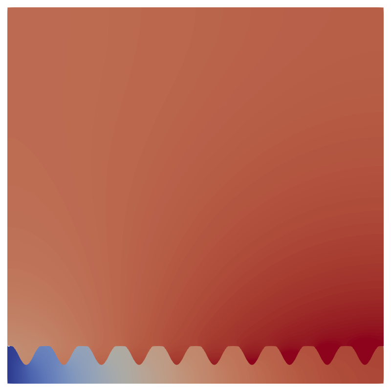
(a) $\varepsilon=0.1$

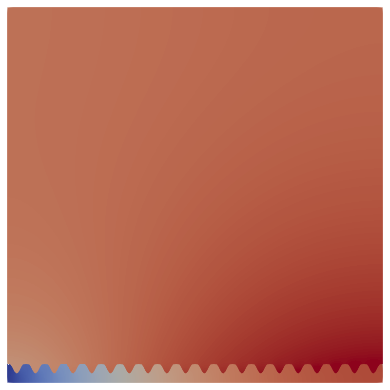
(b) $\varepsilon=0.05$

(c) $\varepsilon=0.01$

(d) Effective

Figure 2: Comparison of the temperature profiles, at $t=5$, for the micro and effective model, with sinusoidal roughness. The effective fluid temperature $\theta^{f}$ is only defined on $(0,1)\times\{0\}$, for visualization purposes the line has been enlarged.

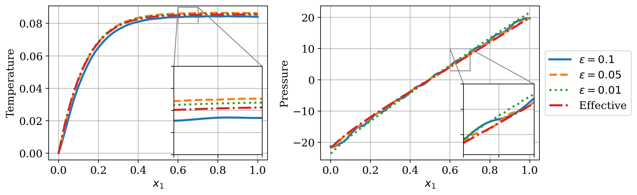
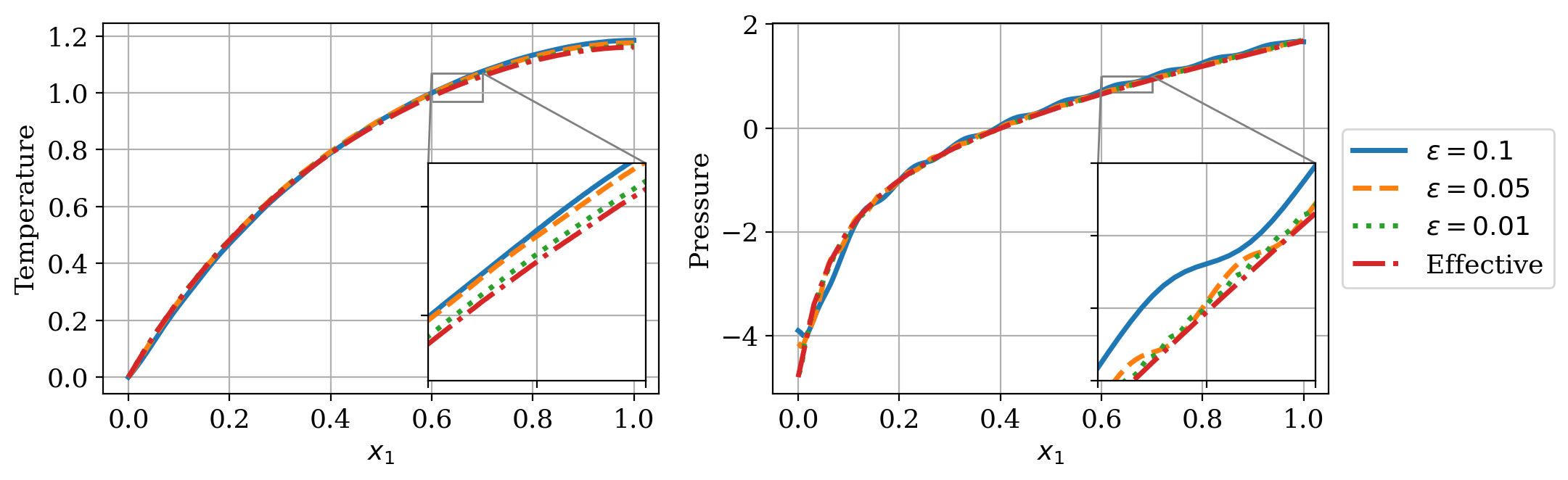
Figure 3: Fluid temperature and pressure along the line $(0,1)\times\{0\}$, compared are the effective model and the micro model for different $\varepsilon$. At the top, the solution at time $t=0.25$, and at the bottom, at time $t=5$. The micro pressure $p_{\varepsilon}$ is multiplied by $\varepsilon^{2}$.

Varying the inflow function. To study how well the effective model captures the influence of the prescribed inflow, we compare different Dirichlet conditions for the roughness given by $\gamma_{\text{sine}}$, $\gamma_{0}=0.5$ and fix $\varepsilon=0.05$. We focus on one $\varepsilon$ to simplify the visualization. The temperature, pressure, and velocity profile, at the time point $t=5$, are visualized in Fig. 4. First, we observe, that, naturally, a higher average fluid flow leads to a cooler system since the heat energy is removed faster from the system. Additionally, for the inflow $u_{\text{BC, quad}}$ and $u_{\text{BC, lin, 2}}$ there is a positive pressure at the inflow since the amount of fluid pressed into the domain is larger than the amount moved by the bottom boundary condition. The homogenized model can capture the influence of the different inflow conditions quite well, regarding temperature and pressure. Even for $u_{\text{BC, lin, 2}}$, which does not directly fulfill the assumptions made in Section 2.3.

Note, that the homogenized model only utilizes the averaged velocity $\bar{u}$, and therefore, no information about the microscopic variations in the velocity field can be obtained.

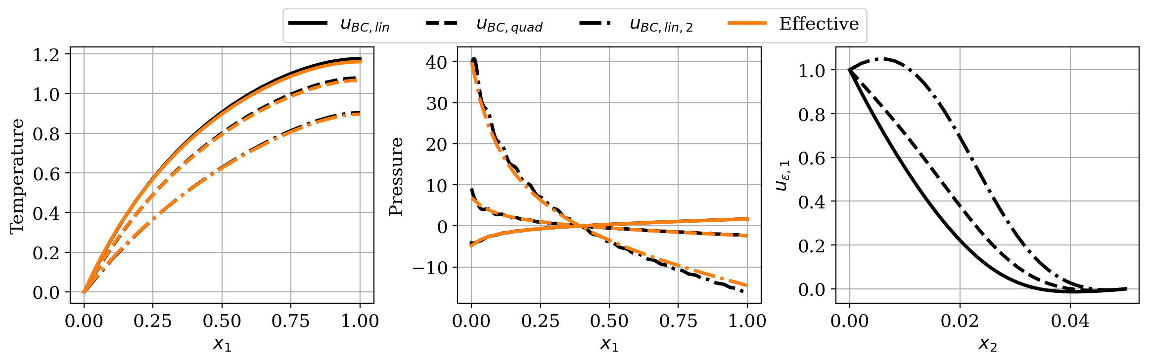
Figure 4: Comparison of the fluid temperature, pressure, and horizontal velocity component for different inflow functions, at $t=5$. In black the micro solution, and in orange the effective results. The temperature and pressure are plotted along the line $(0,1)\times\{0\}$, while the velocity is visualized along $\{0.5\}\times(0,\varepsilon)$.

Varying the grain height $\gamma_{0}$. Next, we investigate the influence of the interface height $\gamma_{0}$. Here, we again focus on the roughness given by $\gamma_{\text{sine}}$ and fix $\varepsilon=0.05$. To only study the influence of $\gamma_{0}$ we use the inflow function $u_{\text{BC, lin, 2}}$ such that effective inflow is independent of $\gamma_{0}$. Similarly, we modify the heat source to $f_{\varepsilon}=\tfrac{1}{|\Gamma|}$ such that the total amount of heat produced averages to one and is independent of $\gamma_{0}$. For the case, $\gamma_{0}=0.1$ are mesh with a resolution of $h=0.01$, respectively $0.01\varepsilon$ in the fluid layer, was needed to obtain stable results. The simulated solutions, again at $t=5$, are presented in Fig. 5. As in the results before, the homogenized model has a good match with the exactly resolved case. The grain height has a big influence on the pressure profile since we have a fixed amount of inflow for all cases, a smaller gap, therefore, leads to higher pressure in the layer. At the same time, the fluid flow in the roughness ”valleys” is reduced, leading to slightly higher temperatures.

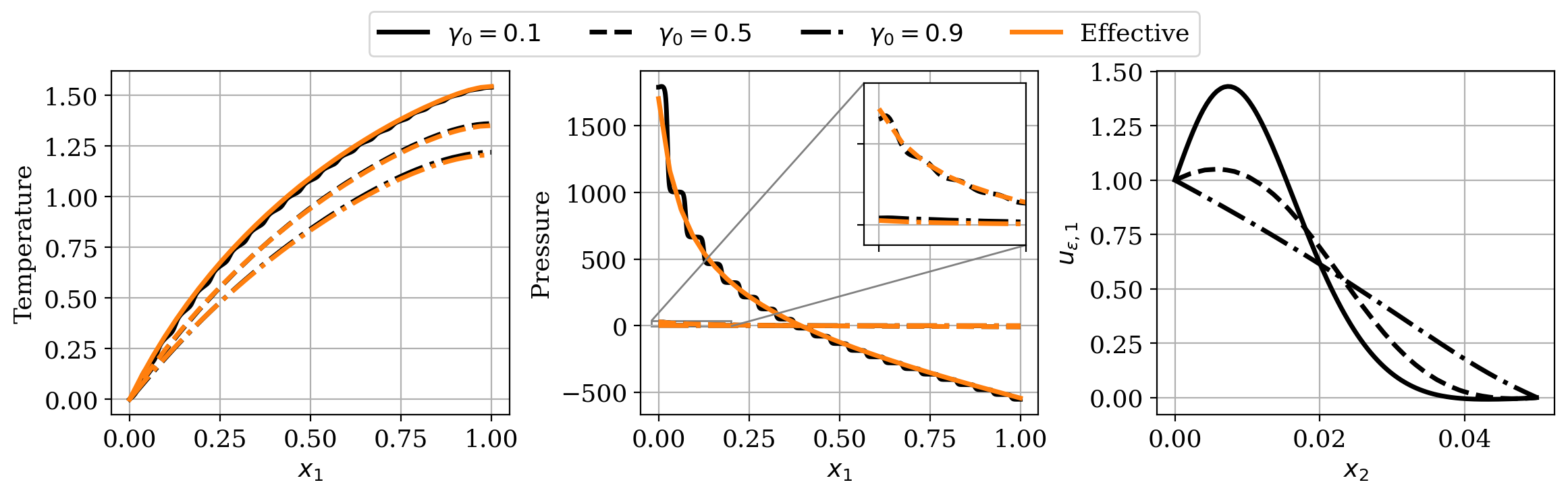
Figure 5: Comparison of the fluid temperature, pressure, and horizontal velocity component for different roughness heights $\gamma_{0}$, at $t=5$. The solution is visualized as in Fig. 4.

Varying the roughness pattern. In the last simulation for the two-dimensional case, we demonstrate the influence of different roughness patterns. We utilize the same setup as in the previous case for varying roughness height but fix $\gamma_{0}$ and compare the differences between $\gamma_{\text{sine}}$ and $\gamma_{\text{rect}}$. As before, we present the results, for the last time step, in Fig. 6. The homogenized model accurately reflects the influence of the roughness pattern on all solution fields. For 2D we can conclude, that the derived effective model yields a good approximation of the resolved micro model and the temperature-dependent viscosity has a, rather large, impact and the pressure profile.

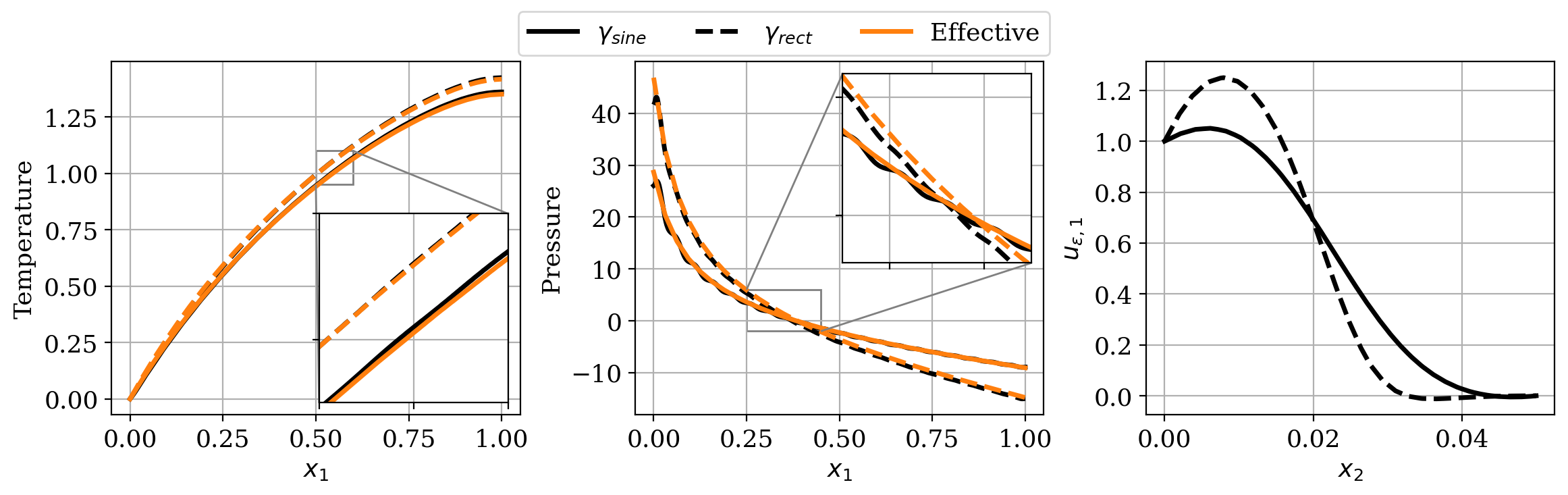
Figure 6: Comparison of the fluid temperature, pressure, and horizontal velocity component for different roughness types, at $t=5$. The solution is visualized as in Fig. 4.

3D simulation study. Lastly, we demonstrate the effects of the temperature-dependent viscosity on the fluid velocity $u$. For this, a three-dimensional setup is required. Unfortunately, this means the resolved microsimulations become computationally expensive and require a lot of memory. Therefore, we only investigate this effect in the homogenized model and the resolved model for $\varepsilon=0.1$. To increase the effect of the temperature-dependent viscosity on the flow field, we see $\kappa^{f}=0.01$ and $C=0.4$. Additionally, we consider a local heat source given by

$$f_{\varepsilon}(x)=\begin{cases}1\quad&\text{, if }x_{2}>0.5\text{ and }|x_{1}-0.5|<0.1,\\ 0&\text{ else}.\end{cases}$$

The inflow is defined by $u_{\text{BC, lin}}$ with $\gamma=0.5$ and $u_{\text{motion}}=(1,0,0)^{T}$. For the roughness we define

$$\gamma=1-0.9\left(\cos{(2\pi(x_{2}-0.5)^{2})}\cos(2\pi(x_{1}-0.25))\right)^{2},$$

so that the effective quantities behave differently in directions $e_{1}$ and $e_{2}$. The corresponding effective parameters are collected in Table 2.

$Z$	$\tilde{\kappa}$	$K$	$\bar{\xi}_{0}$
	$\left(\begin{array}[]{cc}0.493&0.0\\ 0.0&0.635\end{array}\right)$	$\left(\begin{array}[]{cc}0.004566&0.0\\ 0.0&0.004947\end{array}\right)$	$\left(\begin{array}[]{c}0.134\\ 0.0\end{array}\right)$

Table 2: Effective parameters for the three-dimensional simulation. The effective values corresponding to dimension $d$ are not listed, since they are zero.

The non-linearity is resolved by splitting up the problem and doing the time stepping for temperature and Stokes problem sequentially. To be precise, we do a time step for the fluid velocity and pressure using the temperature from the previous time step, followed by a time step of the temperature problem with the velocity of the new time step.

The simulation results at three distinct time steps are presented in Fig. 8. The effect of the temperature-dependent viscosity can be observed in the flow profile. In the beginning ($t=0.05$), the temperature is more or less constant, so there is a uniform velocity field. The viscosity decreases locally ($t=1.85$) due to localized heat source and the fluid flows diagonally upwards towards the area of lower viscosity. As soon as the temperature has spread through the advection, the observed effect slightly decreases $(t=5.0)$. We can conclude, that the temperature-dependent viscosity leads to interesting effects, and working with the non-linear problem is justified. This effect appears in both models but is easier to recognize, in Fig. 8, for the homogenized case, since the mesh there does not need to resolve the roughness and has a uniform structure. Again, the effective model yields a good approximation of the resolved micromodel, while needing less computation time.

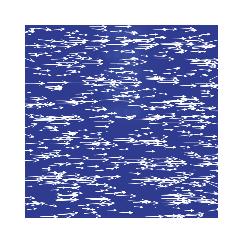
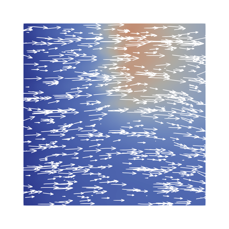
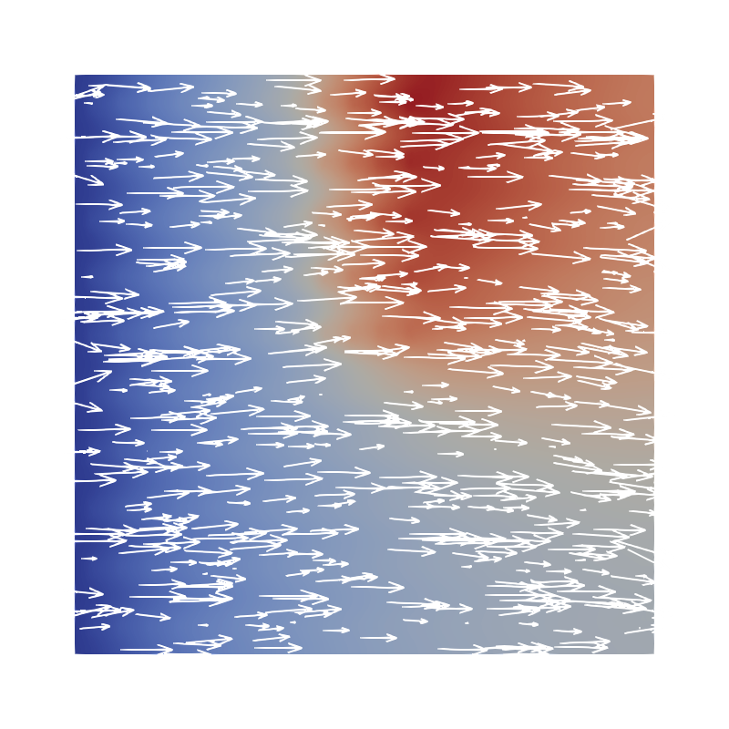
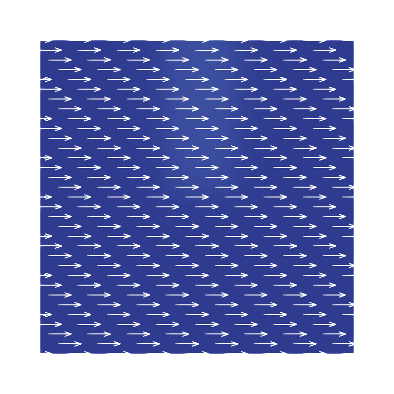
(a) $t=0.05$

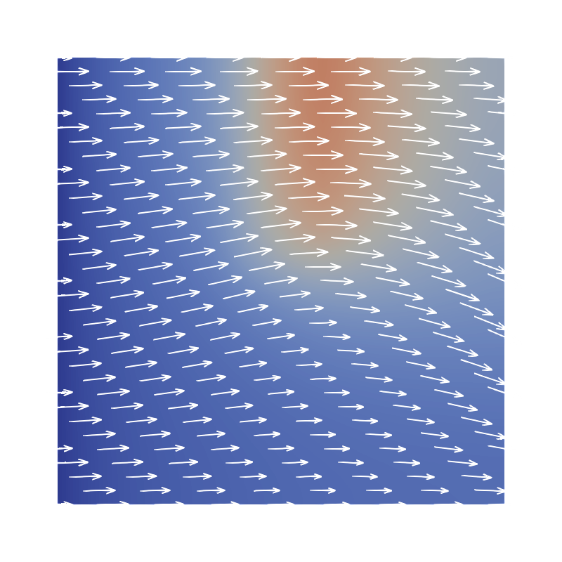
(b) $t=1.85$

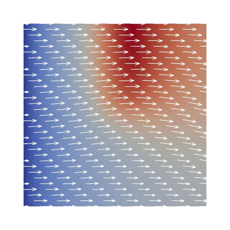
(c) $t=5.0$

Figure 8: Temperature and velocity profile for the three-dimensional setup, at different snapshots in time. At the top, is the resolved micro model, and at the bottom, is the effective model. For the micro model, a cross-section at $x_{3}=0.01$ is visualized, such that the flow profile is better recognizable. Note, that the mesh for the micro model needs to resolve the roughness structure and therefore the representation of the velocity profile is rather disorganized, while in the effective case, we can use a uniform mesh.

6 Conclusion

We investigated the effective behavior of a non-linear Stokes-temperature system in a thin layer, where the non-linearity arises through the convection term in the heat equation and temperature-dependent viscosity. With the concept of two-scale convergence, an effective model was derived, where for the fluid we recovered the results of [10], plus an additional coupling with the temperature field. While the effective fluid temperature is given by an interface function. Multiple simulation results confirm the derived model and show that the temperature-dependent viscosity also plays a non-negligible role in the limit $\varepsilon\to 0$.

In reality, additional parameters are temperature-dependent, for example, the conductivity $\kappa$ or heat exchange parameter $\alpha$. We focused solely on the viscosity, to mainly simplify the notation. Similar to the present approach, e.g. decoupling the system and showing the existence of solutions with a fixed point argument, temperature-dependent $\kappa$ and $\alpha$ could be handled as well. Of course, with fitting assumptions for the parameters. Another aspect that could be investigated further is the current $\varepsilon$-scaling of $\kappa$ in the thin layer. Removing this scaling complicates the analysis, and may lead to an effective equation without diffusion on the interface $\Sigma$.

Regarding the motivating application of a grinding process, we could derive a justification for models used in the literature; see [26]. Currently, we assume the nonrealistic scenario of periodic roughness. In future research, we plan to extend this model to real grinding wheel and workpiece surfaces. Then, we will also investigate the importance of including microstructures in regard to the whole process.

Conflict of interest

The authors declare that there is no conflict of interest.

References

- [1] G. A. Homogenization and two scale convergence. SIAM J. Math. Anal., 23(6):1482–1518, 1992.
- [2] E. Acerbi, V. ChiadòPiat, G. Dal Maso, and D. Percivale. An extension theorem from connected sets, and homogenization in general periodic domains. Nonlinear Analysis: Theory, Methods & Applications, 18(5):481–496, 1992.
- [3] G. Allaire. Homogenization of the Stokes flow in a connected porous medium. Asymptotic Analysis, 2:203–222, 1989. 3.
- [4] A. Almqvist, E. Burtseva, K. Rajagopal, and P. Wall. On lower-dimensional models of thin film flow, part c: Derivation of a Reynolds type of equation for fluids with temperature and pressure dependent viscosity. Proceedings of the Institution of Mechanical Engineers, Part J: Journal of Engineering Tribology, 237:135065012211352, 12 2022.
- [5] A. Almqvist, E. Essel, L.-E. Persson, and P. Wall. Homogenization of the unstationary incompressible reynolds equation. Tribology International, 40(9):1344–1350, 2007.
- [6] M. S. Alnaes, J. Blechta, J. Hake, A. Johansson, B. Kehlet, A. Logg, C. Richardson, J. Ring, M. E. Rognes, and G. N. Wells. The FEniCS project version 1.5. Arch. Num. Soft., 3, 2015.
- [7] F. Alouges. Introduction to periodic homogenization. Interdisciplinary Information Sciences, 22:147–186, 12 2016.
- [8] R. Araya, C. Cárcamo, and A. H. Poza. A stabilized finite element method for the Stokes–Temperature coupled problem. Applied Numerical Mathematics, 187:24–49, 2023.
- [9] G. Bayada and M. Chambat. The transition between the Stokes equations and the Reynolds equation: A mathematical proof. Applied Mathematics and Optimization, 14(1):73–93, Apr 1986.
- [10] G. Bayada and M. Chambat. Homogenization of the Stokes system in a thin film flow with rapidly varying thickness. RAIRO. Modélisation Mathématique et Analyse Numérique, 23, 01 1989.
- [11] N. Benhaboucha, M. Chambat, and I. Ciuperca. Asymptotic behaviour of pressure and stresses in a thin film flow with a rough boundary. Quarterly of Applied Mathematics, 63(2):369–400, 2005.
- [12] A. Bhattacharya, M. Gahn, and M. Neuss-Radu. Effective transmission conditions for reaction–diffusion processes in domains separated by thin channels. Applicable Analysis, 101(6):1896–1910, 2022.
- [13] A. N. Brooks and T. J. Hughes. Streamline upwind/petrov-galerkin formulations for convection dominated flows with particular emphasis on the incompressible Navier-Stokes equations. Computer Methods in Applied Mechanics and Engineering, 32(1):199–259, 1982.
- [14] L. Chupin and S. Martin. Rigorous derivation of the thin film approximation with roughness-induced correctors. SIAM Journal on Mathematical Analysis, 44(4):3041–3070, 2012.
- [15] R. L. de Paiva, R. de Souza Ruzzi, and R. B. da Silva. An approach to reduce thermal damages on grinding of bearing steel by controlling cutting fluid temperature. Metals, 11(10), 2021.
- [16] P. Donato, E. Jose, and D. Onofrei. Asymptotic analysis of a multiscale parabolic problem with a rough fast oscillating interface. Archive of Applied Mechanics, 89:1–29, 03 2019.
- [17] M. Eden and T. Freudenberg. Effective heat transfer between a porous medium and a fluid layer: Homogenization and simulation. Multiscale Modeling & Simulation, 22(2):752–783, 2024.
- [18] L. Evans. Partial Differential Equations. Graduate studies in mathematics. American Mathematical Society, 1998.
- [19] J. Fabricius and M. Gahn. Homogenization and dimension reduction of the Stokes problem with Navier-slip condition in thin perforated layers. Multiscale Modeling & Simulation, 21(4):1502–1533, 2023.
- [20] J. Fabricius, A. Tsandzana, F. Perez-Rafols, and P. Wall. A Comparison of the Roughness Regimes in Hydrodynamic Lubrication. Journal of Tribology, 139(5):051702, 05 2017.
- [21] T. Freudenberg and M. Eden. Homogenization and simulation of heat transfer through a thin grain layer. Netw. Heterog. Media (accepted), 2024. arxiv.org/abs/2312.02704.
- [22] M. Gahn, M. Neuss-Radu, and W. Jäger. Two-scale tools for homogenization and dimension reduction of perforated thin layers: Extensions, Korn-inequalities, and two-scale compactness of scale-dependent sets in Sobolev spaces, 2021. Preprint, arxiv.org/abs/2112.00559.
- [23] M. Gahn, M. Neuss-Radu, and P. Knabner. Derivation of effective transmission conditions for domains separated by a membrane for different scaling of membrane diffusivity. Discrete and Continuous Dynamical Systems - Series S, 10:773–797, 04 2017.
- [24] C. Geuzaine and J.-F. Remacle. Gmsh: A 3-d finite element mesh generator with built-in pre- and post-processing facilities. Int. J. Numer. Methods. Eng., 79:1309 – 1331, 09 2009.
- [25] V. Girault and P.-A. Raviart. Finite element approximation of the Navier-Stokes equations. Springer, 1981.
- [26] R. Gu, M. Shillor, G. Barber, and T. Jen. Thermal analysis of the grinding process. Mathematical and Computer Modelling, 39(9):991–1003, 2004.
- [27] F. Klocke and A. Kuchle. Manufacturing Processes 2: Grinding, Honing, Lapping. RWTHedition. Springer Berlin Heidelberg, 2009.
- [28] D. Lukkassen, A. Meidell, and P. Wall. Analysis of the effects of rough surfaces in compressible thin film flow by homogenization. International Journal of Engineering Science, 49(5):369–377, 2011.
- [29] S. Marusic and E. Marusic-Paloka. Two-scale convergence for thin domains and its applications to some lower-dimensional models in fluid mechanics. Asymptotic Analysis, 23:23–57, 05 2000.
- [30] Y. Min, M. Kong, C. Li, Y.-Z. Long, Y. B. Zhang, S. Sharma, R. Li, T. Gao, M. Liu, X. Cui, X. Wang, X. Ma, and Y. Yang. Temperature field model in surface grinding: A comparative assessment. International Journal of Extreme Manufacturing, 5, 09 2023.
- [31] M. Neuss-Radu and W. Jäger. Effective transmission conditions for reaction-diffusion processes in domains separated by an interface. SIAM Journal on Mathematical Analysis, 39(3):687–720, 2007.
- [32] B. E. Poling, J. M. Prausnitz, and J. P. O’Connell. Properties of Gases and Liquids. McGraw-Hill Education, New York, 5th edition edition, 2001.
- [33] C. Pérez, J.-M. Thomas, S. Blancher, and R. Creff. The steady Navier–Stokes/energy system with temperature‐dependent viscosity—part 1: Analysis of the continuous problem. International Journal for Numerical Methods in Fluids, 56:63 – 89, 01 2008.
- [34] O. Reynolds. On the theory of lubrication and its application to mr. beauchamp tower’s experiments, including an experimental determination of the viscosity of olive oil. Philosophical Transactions of the Royal Society of London, 177:157–234, 1886.
- [35] J. Schauder. Der Fixpunktsatz in Funktionalraümen. Studia Mathematica, 2(1):171–180, 1930.
- [36] R. Showalter. Montone Operators in Banach Space and Nonlinear Partial Differential Equations, volume 49. Mathematical Surveys and Monographs, 01 1997.
- [37] H. Tönshoff, J. Peters, I. Inasaki, and T. Paul. Modelling and simulation of grinding processes. CIRP Annals, 41(2):677–688, 1992.
- [38] P. Wiederkehr, A. Grimmert, I. Heining, T. Siebrecht, and F. Wöste. Potentials of grinding process simulations for the analysis of individual grain engagement and complete grinding processes. Frontiers in Manufacturing Technology, 2, 2023.
- [39] F. Wiesener, B. Bergmann, M. Wichmann, M. Eden, T. Freudenberg, and A. Schmidt. Modeling of heat transfer in tool grinding for multiscale simulations. Procedia CIRP, 117:269–274, 2023.
- [40] Y. Zheng, C. Wang, Y. Zhang, and F. Meng. Study on temperature of cylindrical wet grinding considering lubrication effect of grinding fluid. The International Journal of Advanced Manufacturing Technology, 121(9):6095–6109, Aug 2022.