Measuring the Dispersion of Discrete Distributions

Abstract

Measuring dispersion is among the most fundamental and ubiquitous concepts in statistics, both in applied and theoretical contexts. In order to ensure that dispersion measures like the standard deviation indeed capture the dispersion of any given distribution, they are by definition required to preserve a stochastic order of dispersion. The most basic order that functions as a foundation underneath the concept of dispersion measures is the so-called dispersive order. However, that order is incompatible with almost all discrete distributions, including all lattice distribution and most empirical distributions. Thus, there is no guarantee that popular measures properly capture the dispersion of these distributions.

In this paper, discrete adaptations of the dispersive order are derived and analyzed. Their derivation is directly informed by key properties of the dispersive order in order to obtain a foundation for the measurement of discrete dispersion that is as similar as possible to the continuous setting. Two slightly different orders are obtained that both have numerous properties that the original dispersive order also has. Their behaviour on well-known families of lattice distribution is generally as expected if the parameter differences are large enough. Most popular dispersion measures preserve both discrete dispersive orders, which rigorously ensures that they are also meaningful in discrete settings. However, the interquantile range preserves neither discrete order, yielding that it should not be used to measure the dispersion of discrete distributions.

Keywords: Dispersion, Discrete distributions, Stochastic orders, Dispersion measures

1 Introduction

The measurement of dispersion is one of the most fundamental concepts in statistics. It is used ubiquitously in mathematical statistics as well as in applied sciences and in theoretical as well as in empirical contexts. Although dispersion measures have at least been used since the beginning of the 19th century [11], their first rigorous definition was given by [3, 4]. They required a dispersion measure $\tau$ to have two defining properties: the first one stipulates its behaviour under affine linear transformations and the second one requires that it preserves a given order of dispersion $\leq_{\text{D}}$ in the sense that $F\leq_{\text{D}}G$ implies $\tau(F)\leq\tau(G)$. The crucial property for the meaningful measurement of dispersion is the second one. Hence, the used dispersion order $\leq_{\text{D}}$ can be understood as a foundation underneath the notion of dispersion.

The dispersive order $\leq_{\text{disp}}$ is the strongest order of dispersion in the literature and therefore imposes the most basic requirement on dispersion measures. The order requires one distribution to be more spread out than another throughout their entire quantile functions in a pointwise sense. Other popular, but weaker, dispersion orders like the dilation order $\leq_{\text{dil}}$ not only compare two distributions using aggegrated quantities, but also inherently favour some dispersion measures that are structurally similar. In the case of the dilation order, the distributions are centred around the mean and therefore dispersion measures like the standard deviation are given an advantage. The dispersive order is also usually chosen as fundamental order for dispersion measures in the literature (see, e.g., [4] and [14]).

A critical shortcoming of the dispersive order is revealed in a innocuous result by [13, Th. 1.7.3 ] that has not garnered any attention in the literature so far. It states that a necessary condition for $F\leq_{\text{disp}}G$ is that the range of the cdf $F$ is a subset of the range of $G$. While this is unproblematic for continuous distributions, it excludes almost all important classes of discrete distributions from being ordered using $\leq_{\text{disp}}$. This includes virtually all lattice distributions and all empirical distributions that either exhibit ties or do not have the same sample size. This means that the use of dispersion measures on discrete distribution does not have a meaningful foundation. A particularly obvious example is given by two discrete uniform distributions, one on the set $\{1,2\}$ and the other on the set $\{1,\ldots,5\}$. Although it is self-evident that the second distribution is more dispersed, the dispersive order does not come to that conclusion. In spite of examples like this, using measures to quantify the dispersion of lattice distributions and empirical distributions is often among the first topics in an introductory statistics course and is commonplace in all kinds of applied sciences. It is the duty of the field of mathematical statistics to ensure that a concept this widely used is well-founded and meaningful.

This paper provides a solution for this problem in form of an adaptation of the dispersive order to discrete distributions. We use two starting points for the derivation of a discrete dispersive order. First, we consider the behaviour of the dispersive order for (absolutely) continuous distributions, where it does not exhibit any problems. Second, its behaviour on the edge of its applicability, so for the small amount of discrete distributions for which it can hold, is taken into account. The derivation yields two slightly different orders that are both viable candidates for the discrete adaptation. Numerous examples throughout the derivation are used to ensure and illustrate both that the derived orders are meaningful and that they are closely related to the original dispersive order.

Following some basics and details on the shortcomings of the dispersive order in Section 2 and the derivation of discrete orders in Section 3, Section 4 provides further arguments for considering the derived orders to be discrete versions of the dispersive order. For that, we show that a number of important properties of the original dispersive order are also fulfilled for both discrete adaptations. However, of two crucial properties (transitivity and equivalence to $\leq_{\text{disp}}$ on the joint area of applicability), each of the two discrete orders only satisfies one. We conjecture that it is impossible to find an order that fulfils both of these crucial properties using a heuristic explanation.

The then following Section 5 is of particular interest as it draws the connection from the world of stochastic orders back to the more application-relevant concept of dispersion measures. Most popular dispersion measures like the standard deviation, the mean absolute deviation from the mean and Gini’s mean difference preserve both of the discrete dispersive orders and therefore measure the dispersion of discrete distributions in a meaningful way. All three results are corollaries of the fact that the dilation order is a weakening of the discrete dispersive orders for discrete distribution; the same is true for the original dispersive order in a continuous setting. unsurprisingly, the dilation order is not helpful for quantile based dispersion measures like the mean absolute deviation from the median or interquantile distances. While the first measure can be shown to preserve the discrete dispersive orders in a different way, any interquantile distance does not preserve them.

This reveals a substantial problem since particularly the interquartile range is a popular measure in descriptive statistics. Using it in the context of empirical or lattice distributions, especially with small supports can lead to fundamental misunderstandings concerning the given data set. Combined with the fact that the counterexamples used to prove this result are rather simple, this provides a convincing and rigorous argument against using this measure in a discrete setting. While this incompatibility has previously been noted in the literature, most recently by [2, p. 1852 ], who deemed the interquantile range not to be a ‘true measure of variability’. However, the given reasoning is that it does not preserve the dilation order, which is not sufficient to infer this kind of statement. For continuous distributions, the interquartile range is indeed a true measure of variability. Furthermore, the fact that it does not preserve the discrete dispersive orders is not dependent upon the used definition of quantiles, which is not unique for discrete distributions.

The derived discrete dispersive orders are applied to a number of popular discrete distributions in Section 6 to find out whether they are systematically ordered in the seemingly evident direction. This is the case, if the parameter difference within the distribution family is large enough. For smaller parameter differences, the situation is less clear, which can be explained by the messy and sparse nature of discrete distributions.

2 The classical foundation of dispersion measurement and its shortcomings for discrete distributions

Let $\mathcal{P}$ denote the set of all real-valued probability distributions and let $\mathcal{Q}\subset\mathcal{P}$ be a suitable subset. We allow $\mathcal{P}$ and subsets thereof to be interpreted as sets of cumulative distribution functions (cdf’s). For each cdf $F\in\mathcal{P}$, we furthermore define the interval

$$D_{F}=\mathbb{R}\setminus F^{-1}(\{0,1\})=\{t\in\mathbb{R}:F(t)\in(0,1)\}.$$

Sets of this kind were also considered in the pioneering works by [17, p. 6 ], who denoted it by $I$, and by [14, p. 155 ], who denoted it by $S_{F}$. If cdf’s $F$ and $G$ are considered, correspondingly distributed random variables are given by $X\sim F$ and $Y\sim G$.

Given an agreed-upon order of dispersion $\leq_{\text{D}}$, the classical definition of a dispersion measure due to [3] is given as follows.

Definition 2.1.

A mapping $\tau:\mathcal{Q}\to[0,\infty)$ is said to be a measure of dispersion, if the following two properties are satisfied:

1. $\tau(aX+b)=|a|\tau(X)$ for all $a,b\in\mathbb{R}$ and $F\in\mathcal{Q}$,

2. $\tau(F)\leq\tau(G)$ for all $F,G\in\mathcal{Q}$ with $F\leq_{\text{D}}G$.

Condition (D1) of Definition 2.1 only imposes restrictions on the dispersion measure values of linearly related distributions and particularly ensures that $\tau$ measures dispersion in a symmetric way. Since condition (D2) is much more crucial, the chosen dispersion order $\leq_{\text{D}}$ acts as the foundation underneath dispersion measures that ensures that they are meaningful. An example of counterintuitive behaviour of measures that do not preserve a corresponding order is given in the context of skewness in [6] and underlines the importance of this order-based definition. The two most popular dispersion orders in the literature are defined as follows [13, see, e.g.,].

Definition 2.2.

Let $F,G\in\mathcal{P}$.

1. $F$ is said to precede $G$ in the dispersive order, in short $F\leq_{\text{disp}}G$, if

   $$F^{-1}(p_{1})-F^{-1}(p_{0})\leq G^{-1}(p_{1})-G^{-1}(p_{0})\quad\forall 0<p_{0}\leq p_{1}<1.$$

2. Let the first moments of $F$ and $G$ exist. Then, $F$ is said to precede $G$ in the dilation order, in short $F\leq_{\text{dil}}G$, if

   $$\mathbb{E}\left[\varphi(X-\mathbb{E}[X])\right]\leq\mathbb{E}\left[\varphi(Y-\mathbb{E}[Y])\right]$$

   for all convex functions $\varphi$ for which the expectations exist.

The dispersive order can be equivalently characterized using Q-Q-plots. $F\leq_{\text{disp}}G$ holds, if and only if any straight line connecting two points in the corresponding Q-Q-plot has a slope of at least one.

The dilation order is closely related to the more well-known convex order, which is defined in the same way without the standardization with respect to the mean. The following proposition contains two helpful properties of the two orders [13, see, e.g.,].

Proposition 2.3.

Let $F,G\in\mathcal{P}$.

1. $F\leq_{\text{dil}}G$ is equivalent to $\pi_{X-\mathbb{E}[X]}(t)\leq\pi_{Y-\mathbb{E}[Y]}(t)$ for all $t\in\mathbb{R}$, where $\pi_{Z}:\mathbb{R}\to[0,\infty),t\mapsto\mathbb{E}[(Z-t)_{+}]$ denotes the stop-loss transform of a random variable $Z$.

2. $F\leq_{\text{disp}}G$ implies $F\leq_{\text{dil}}G$.

For the definition of dispersion measures as given in 2.1, the dispersive order $\leq_{\text{disp}}$ is usually chosen as the foundational order (see, e.g., [4] and [14]). One major reason for this choice is that $\leq_{\text{disp}}$ is the strongest order of dispersion that is commonly considered in the literature; in particular, it is stronger that the dilation order $\leq_{\text{dil}}$. While $F\leq_{\text{disp}}G$ means that $G$ is more dispersed than $F$ in a pointwise fashion, $F\leq_{\text{dil}}G$ represents a comparison of averages that can, e.g., be expressed via the stop-loss transform. Thus, $\leq_{\text{disp}}$ imposes a minimal requirement on the notion of a dispersion measure. If the dispersive order deems one distribution to be more dispersed than another, this statement is strong enough that every reasonable dispersion measure must share this preference. A second major reason is that the dispersive order does not inherently center the considered distributions around some measure of central location and therefore does not inherently prefer certain dispersion measures to others. For two distributions to be ordered with respect to $\leq_{\text{disp}}$, one must spread out more than the other in a pointwise sense. On the other hand, the dilation order compares the dispersion of two distribution by first centering them around the mean, thus inherently favouring corresponding dispersion measures like the standard deviation. So, when referring to measures of dispersion or dispersion measures throughout this paper, we mean mappings as defined by Definition 2.1 with $\leq_{\text{disp}}$ in the role of $\leq_{\text{D}}$.

The following result concerning the dispersive order is given by [13, p. 41 ].

Proposition 2.4.

Let $F,G\in\mathcal{P}$. Then, $F\leq_{\text{disp}}G$ implies $F(D_{F})\subseteq G(D_{G})$.

Conversely, this means that, if neither range of two cdf’s is a subset of the range of the other cdf, the two distributions are not ordered with respect to $\leq_{\text{disp}}$. This does not present an obstacle for continuous distributions since the range of their cdf’s always equals the entire unit interval. Discrete cdf’s, however, take at most countably many values. This means that, if two discrete ranges were picked at random (via independent uniformly distributed random variables), the probability for the ranges to even coincide in one point would be zero. This problem persists when we consider specific families of distributions like the binomial, Poisson or geometric distributions. An exception is given by specific classes of empirical distributions. In particular, every pair of non-tied empirical distributions with the same sample size satisfies the condition in Proposition 2.4.

However, it is very easy to find examples where one distribution is unambiguously more dispersed than the other, but neither $F(D_{F})\subseteq G(D_{G})$ nor $G(D_{G})\subseteq F(D_{F})$ holds, which means that the two distributions are not comparable with respect to $\leq_{\text{disp}}$. A particularly simple example is given in the following.

Example 2.5.

Let $X\sim\mathcal{U}(\{1,2\})$, $Y\sim\mathcal{U}(\{1,\ldots,5\})$ and $\tilde{Y}\sim\mathcal{U}(\{1,\ldots,4\}$. We have $F(D_{F})=\{\tfrac{1}{2}\}$ and $G(D_{G})=\{\tfrac{1}{5},\tfrac{2}{5},\tfrac{3}{5},\tfrac{4}{5}\}$, thus, $F\not\leq_{\text{disp}}G$ (and $G\not\leq_{\text{disp}}F$). On the other hand, it is easy to show $X\leq_{\text{disp}}\tilde{Y}$. In particular, this can be seen by observing the corresponding Q-Q-plot in Figure 1.

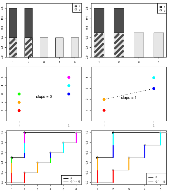
Figure 1: Different illustrations of the two pairs of distributions considered in Example 2.5: $X\sim\mathcal{U}(\{1,2\})$ and $Y\sim\mathcal{U}(\{1,\ldots,5\})$ in the left panels; $X$ and $\tilde{Y}\sim\mathcal{U}(\{1,2,3,4\})$ in the right panels. Upper: barplots of pmf’s; Middle: Q-Q-plots; Lower: colour-coded cdf’s.

The pmf’s of $X$ and $Y$ are given in the upper left panel and the pmf’s of $X$ and $\tilde{Y}$ are given in the upper right panel. It is obvious that both $X\leq_{\text{D}}Y$ and $X\leq_{\text{D}}\tilde{Y}$ should hold for any sensible dispersion order $\leq_{\text{D}}$. The difference between $X$ and $Y$ is even larger than that between $X$ and $\tilde{Y}$, yet $X\not\leq_{\text{disp}}Y$ and $X\leq_{\text{disp}}\tilde{Y}$. The reason for this becomes more obvious by observing the corresponding Q-Q-plots in the two middle panels of Figure 1. The critical point in both Q-Q-plots is the jump of $F^{-1}$ from the value $1$ to the value $2$. On the left side, the slope between the two corresponding points is zero, which contradicts $X\leq_{\text{disp}}Y$; on the right side, the slope between these two points is one, and therefore $X\leq_{\text{disp}}\tilde{Y}$ is true.

The difference in the two Q-Q-plots can be explained by the comparison of the cdf’s, which are depicted in the lower panels of Figure 1. It is colour-coded into the cdf’s how the probability mass is shared between the different points in the supports of both distributions. Since this is essentially what is represented by the Q-Q-plots, the colours of the points in the Q-Q-plots correspond to those used for the cdf’s. The reason for the slope of zero in the Q-Q-plot on the left side is that a smaller jump of $G$ lies in between two larger jumps of $F$. This is not the case on the right side precisely because the condition $F(D_{F})\subseteq G(D_{G})$ is fulfilled.

The fact that constellations as in Example 2.5 exist, implies that $\leq_{\text{disp}}$ does not order discrete distributions sufficiently well with respect to dispersion. Recalling Definition 2.1, this leaves the concept of dispersion on discrete distributions without a foundation. In particular, the idea that popular dispersion measures like the standard deviation, the quantile distance and many others actually measure dispersion does not have any basis in a discrete setting.

The above observations suggest that a rigorous foundation of dispersion for discrete distributions requires an order that has the properties of the dispersive order but is more suitable for the discrete setting. Somewhat surprisingly, this gap in the foundation of dispersion measures has neither been explicitly pointed out nor tackled in the literature. In many important works on the topic, e.g. in [14], attention is a priori restriced to continuous distributions with sufficient differentiability properties. In a recent publication by [12], a modified dispersive order for empirical distributions is defined, but the rest of the paper focuses on a similarly modified version of the usual stochastic order. Furthermore, as mentioned after Proposition 2.4, the problem of the dispersive order with discrete distribution is a lot less severe for empirical distributions with the same sample size, to which the approach by [12] is restricted.

Overall, the set of distributions that lack a foundation with respect to the measurement of dispersion still includes empirical distributions with differing sample sizes and all lattice distributions. Since a concept this widely used should not lack any rigour, Section 3 is dedicated to establishing this kind of order.

3 Finding a discrete dispersive order: Keep what works, replace what is broken

Let $\mathcal{D}\subset\mathcal{P}$ denote the set of discrete distributions. Since $\mathcal{D}$ contains a number of difficult to handle distributions with virtually no practical use, we limit our considerations to the class of purposive discrete distributions given in the following definition along with a number of subclasses.

Definition 3.1.

Let $F\in\mathcal{D}$ be a cdf with pmf $f$ and let $X\sim F$. The class of purposive discrete distributions $\mathcal{D}_{0}\subseteq\mathcal{D}$ is defined by

$$F\in\mathcal{D}_{0}\Leftrightarrow \ \operatorname{supp}(F)\text{ is order-isomorphic to a subset of }\mathbb{Z}\text{ with at least two elements}$$

$$\Leftrightarrow \ \exists A\subseteq\mathbb{Z},|A|\geq 2,\text{bijection }\varphi:\operatorname{supp}(F)\to A\text{ such that}$$

$$\ x\leq y\Leftrightarrow\varphi(x)\leq\varphi(y)\ \forall x,y\in\operatorname{supp}(F).$$

Note that there indeed exist non-degenerate discrete distributions in $\mathcal{D}\setminus\mathcal{D}_{0}$, i.e. discrete distributions that are not order-isomorphic to a subset of the whole numbers. However, the class $\mathcal{D}_{0}$ contains all lattice distributions and empirical distributions, which are the most frequently used kinds of discrete distributions.

The following result, which is crucial for the remainder of this work, is only valid for distributions in $\mathcal{D}_{0}$.

Proposition 3.2.

Define

$$\mathbb{I}=\{\mathbb{Z},\mathbb{N},-\mathbb{N}\}\cup\{\{1,\ldots,n\}:n\in\mathbb{N}_{\geq 2}\}$$

and

$$\mathbb{S}_{A}= \;\Bigg{\{}(x_{j},p_{j})_{j\in A}\subseteq\mathbb{R}\times(0,1]:x_{i}<x_{j}\text{ for }i<j,\ p_{j}>0\text{ for }j\in A,\ \sum_{j\in A}p_{j}=1\Bigg{\}}$$

for $$A\in\mathbb{I}\setminus\mathbb{Z}$$ as well as

$$\mathbb{S}_{\mathbb{Z}}= \;\Bigg{\{}(x_{j},p_{j})_{j\in\mathbb{Z}}\subseteq\mathbb{R}\times(0,1]:x_{i}<x_{j}\text{ for }i<j,\ p_{j}>0\text{ for }j\in\mathbb{Z},\ \sum_{j\in\mathbb{Z}}p_{j}=1,$$

$$\;\hphantom{\Bigg{\{}(x_{j},p_{j})_{j\in\mathbb{Z}}\subseteq\mathbb{R}\times(0,1]:}\inf\{j\in\mathbb{Z}:\sum_{i\leq j}p_{i}\geq\tfrac{1}{2}\}=0\Bigg{\}}.$$

For any $F\in\mathcal{D}_{0}$, there exists a unique index set $A\in\mathbb{I}$ that is order-isomorphic to $\operatorname{supp}(F)$, and there exists a unique sequence $(x_{j},p_{j})_{j\in A}\in\mathbb{S}_{A}$ such that $\mathbb{P}(X=x_{j})=p_{j}$ for all $j\in A$. This unique association is denoted by $F\;\hat{=}\;\left(A,(x_{j},p_{j})_{j\in A}\right)$. $A$ is said to be the indexing set of $F$ and $(x_{j},p_{j})_{j\in A}$ is said to be the identifying sequence of $F$.

Note that if $\mathbb{S}_{\mathbb{Z}}$ were of the same structure as $\mathbb{S}_{A}$ for $A\neq\mathbb{Z}$, $F$ could only be uniquely identified up to an arbitrary index shift of the identifying sequence. The additional condition in $\mathbb{S}_{\mathbb{Z}}$ assures that the index $0$ relates to the median and thereby fixes the sequence.

Throughout the remainder of this paper, let $F\;\hat{=}\;\left(A,(x_{j},p_{j})_{j\in A}\right)$ and $G\;\hat{=}\;\left(B,(y_{j},q_{j})_{j\in B}\right)$. Furthermore, we establish the conventions $x_{a}=-\infty$ and $F(x_{a})=0$ for $a<\min A$ as well as $x_{a}=\infty$ and $F(x_{a})=1$ for $a>\max A$, provided that the minimum and the maximum exist, respectively.

The goal now is to construct a dispersion order that is meaningfully applicable to discrete distributions and therein assumes the same role as the dispersive order $\leq_{\text{disp}}$ has for continuous distribution. This presents us with two starting points for our derivation. The first is to find a representation of the dispersive order for continuous distributions that has an easily applicable discrete analogue. The second is to find out what exactly is required by the original dispersive order $\leq_{\text{disp}}$ at the edge of its applicability to discrete distributions.

We start out by considering the second starting point, postponing the first one to Section 3.1. To this end, the following result refines Proposition 2.4 for discrete distributions as is gives an equivalent characterization of $\leq_{\text{disp}}$ in that case. The one-dimensional Lebesgue measure is denoted by $\lambda^{1}$. Consequently, for any $F\in\mathcal{D}_{0}$ and $p\in F(D_{F})$, $\lambda^{1}(F^{-1}(\{p\}))$ describes “how long” $F$ assumes the value $p$.

Proposition 3.3.

Let $F,G\in\mathcal{D}$. Then $F\leq_{disp}G$ is equivalent to

$$F(D_{F})\subseteq G(D_{G})\quad\text{and}\quad\lambda^{1}(F^{-1}(\{p\}))\leq\lambda^{1}(G^{-1}(\{p\}))\ \forall p\in F(D_{F}).$$

Using this characterization, the following examples illustrate how the dispersive order manifests itself specifically on some of the distribution classes given in Definition 3.1.

Example 3.4.

1. Let $F$ and $G$ be two non-tied empirical cdf’s of the same sample size $n\in\mathbb{N}_{\geq 2}$. Then there exist $x,y\in\mathbb{R}^{n}$ with $x_{i}<x_{i+1}$ and $y_{i}<y_{i+1}$ for all $i\in\{1,\ldots,{n-1}\}$ such that $\mathbb{P}(X=x_{i})=\tfrac{1}{n}=\mathbb{P}(Y=y_{i})$ for all $i\in\{1,\ldots,{n}\}$. Because of $F(D_{F})=G(D_{G})=\{\tfrac{i}{n}:i\in\{1,\ldots,{n-1}\}\}$, the following equivalence holds

   $$F\leq_{\text{disp}}G \Leftrightarrow\lambda^{1}(F^{-1}(\{\tfrac{i}{n}\}))\leq\lambda^{1}(G^{-1}(\{\tfrac{i}{n}\}))\quad\forall i\in\{1,\ldots,{n-1}\}$$

   $$\Leftrightarrow x_{i+1}-x_{i}\leq y_{i+1}-y_{i}\quad\forall i\in\{1,\ldots,{n-1}\}.$$

   This means that $G$ is at least as dispersed as $F$, if and only if the distance between every pair of neighbouring points in the support of $F$ is smaller than between the corresponding pair in the support of $F$. Particularly, $y_{j+1}-y_{j}<x_{i+1}-x_{i}$ for $i\neq j$ does not contradict $F\leq_{\text{disp}}G$.

2. Let $F$ and $G$ be empirical cdf’s of the same sample size $n\in\mathbb{N}_{\geq 2}$ with $G$ having no ties and $F$ having exactly one tie. Hence, there exists a unique $i_{0}\in\{1,\ldots,{n-1}\}$ such that $x_{i}<x_{i+1}$ for $i\neq i_{0}$ and $x_{i_{0}}=x_{i_{0}+1}$ holds for the defining vector $x\in\mathbb{R}^{n}$ of $F$. It follows that $F(D_{F})=G(D_{G})\setminus\{\tfrac{i_{0}}{n}\}\subset G(D_{G})$ and therefore

   $$F\leq_{\text{disp}}G \Leftrightarrow\lambda^{1}(F^{-1}(\{\tfrac{i}{n}\}))\leq\lambda^{1}(G^{-1}(\{\tfrac{i}{n}\}))\quad\forall i\in\{1,\ldots,{n-1}\}\setminus\{i_{0}\}$$

   $$\Leftrightarrow x_{i+1}-x_{i}\leq y_{i+1}-y_{i}\quad\forall i\in\{1,\ldots,{n-1}\}\setminus\{i_{0}\}.$$

   Once again, the distances between neighbouring pairs of points in the supports of $F$ and $G$ are compared. Which pairs of points are compared depends on the value that the corresponding cdf takes on the interval between the points. For example, if $i_{0}\neq 1$, the difference $x_{2}-x_{1}$ is compared to $y_{2}-y_{1}$ since $F((x_{1},x_{2}))=\{\tfrac{1}{n}\}=G((y_{1},y_{2}))$. Note that the interval length $y_{i_{0}+1}-y_{i_{0}}$ is not compared to any interval length of $F$.

3. Let $F$ $G$ be the cdf’s of two lattice distribution on the same grid. Then there exist $a,b\in\mathbb{R}$, $c>0$ and $A,B\in\mathbb{I}$ such that $\operatorname{supp}(F)=cA+a$ and $\operatorname{supp}(G)=cB+b$. It immediately follows for all $p\in F(D_{F})=F(\operatorname{supp}(F))\setminus\{1\}$ that

   $$\lambda^{1}(F^{-1}(\{p\}))=a=\lambda^{1}(G^{-1}(\{p\})).$$

   Thus, the statement of Proposition 3.3 simplifies to

   $$F\leq_{\text{disp}}G\Leftrightarrow F(D_{F})\subseteq G(D_{G}).$$

Proposition 3.3 specifies how any pair of discrete distributions can be compared with respect to dispersion. The dispersive order can only order pairs of cdf’s within the set $\{(F,G)\in(\mathcal{D}_{0})^{2}:F(D_{F})\subseteq G(D_{G})\text{ or }G(D_{G})\subseteq F(D_{F})\}$ with respect to dispersion. For the pairs in this set, the first components of the identifying sequences (i.e. the jump points) are arbitrary, while the second components of the sequence (i.e. the jump heights) are mostly fixed. We now turn our attention to a class of distributions, for which the first components of the identifying sequence are mostly fixed while the second components are arbitrary. Afterwards, the goal is to unite the two methodologies in some way to enable us to compare two purposive discrete distributions with respect to their dispersions.

3.1 Comparing jump heights

Two discrete cdf’s $F$ and $G$ cannot be ordered with respect to $\leq_{\text{disp}}$, if neither $F(D_{F})\subseteq G(D_{G})$ nor $G(D_{G})\subseteq F(D_{F})$ holds. However, it is not difficult to find an example where neither inclusion holds but one distribution is unambiguously more dispersed than the other, as evidenced by Example 2.5. The basic idea for how to compare $F$ and $G$ with respect to dispersion in this kind of situation is obtained through one of the starting points discussed before Proposition 3.3. Specifically, the idea is to modify a characterization of $\leq_{\text{disp}}$ for sufficiently regular continuous distributions in such a way that it is applicable to discrete distributions.

According to [14, p. 157 ], $F\leq_{\text{disp}}G$ is equivalent to $(G^{-1}\circ F)^{\prime}\geq 1$, if $F$ and $G$ have interval support and are differentiable. Thus, $F\leq_{\text{disp}}G$ holds if and only if

$$f(F^{-1}(p))\leq g(G^{-1}(p))\quad\forall p\in(0,1),$$ (1)

where $f$ and $g$ denote the Lebesgue densities of $F$ and $G$. The discrete analogue of Lebesgue densities for absolutely continuous distributions are pmf’s, which are also densities, only with respect to a suitable counting measure. Our proposed discrete generalization of the dispersion order is therefore obtained by taking characterization (1) of $\leq_{\text{disp}}$ and replacing the Lebesgue densities with the respective pmf’s. Since the values of a pmf are the jump heights of the corresponding cdf, this gives a requirement concerning the second components of the identifying sequences. We mostly fix the first components of the identifying sequences by assuming

$$x_{a}-x_{a-1}\leq y_{b}-y_{b-1}\quad\forall a\in A\setminus\{\min A\},b\in B\setminus\{\min B\},$$ (2)

For any set $M$ with non-existent minimum, we define $\{\min M\}=\emptyset$; an analogous rule holds for maximums. This means that every interval, on which $G$ is constant, is at least as long as any interval, on which $F$ is constant. Since this puts more distance between the points in the support of $G$ than between those in the support of $F$, thus intuitively makes $G$ more dispersed. Condition (2) is obviously equivalent to

$$\sup_{a\in A\setminus\{\min A\}}(x_{a}-x_{a-1})\leq\inf_{b\in B\setminus\{\min B\}}(y_{b}-y_{b-1}).$$ (3)

With the rather strict condition (2)/(3), we come to our first definition of a discrete version of the dispersive order. Other versions of this order that are weakened with respect to the requirements on the supports, are presented at a later point.

Definition 3.5.

Let $F,G\in\mathcal{D}_{0}$ have the pmf’s $f,g$. Then, $G$ is said to be at least as discretely dispersed as $F$, denoted by $F\leq_{\text{disp}}^{\text{disc}}G$, if (2) is satisfied and

$$g(G^{-1}(p))\leq f(F^{-1}(p))\quad\forall p\in(0,1).$$ (4)

We first apply this definition to the situation in Example 2.5 for which the original dispersive order is not sufficient. This is done in order to find out whether $\leq_{\text{disp}}^{\text{disc}}$ is a suitable idea for its intended purpose.

Example 3.6.

1. Continuation of Example 2.5: Condition (2) is satisfied since $x_{a}-x_{a-1}=1=y_{b}-y_{b-1}$ holds for all $a\in A\setminus\{\min A\},b\in B\setminus\{\min B\}$. Because of $\mathrm{range}(F^{-1})=\operatorname{supp}(F)$ and $\mathrm{range}(G^{-1})=\operatorname{supp}(G)$ and since $f$ is constantly equal to $\frac{1}{2}$ on its support and $g$ is constantly equal to $\frac{1}{5}$ on its support, we obtain

   $$g(G^{-1}(p))=\frac{1}{5}\leq\frac{1}{2}=f(F^{-1}(p))\quad\forall p\in(0,1).$$

   Thus, $F\leq_{\text{disp}}^{\text{disc}}G$ holds as anticipated.

2. The first observation from part a) can be generalized to the entire set of lattice distributions. For that, let $F$ and $G$ be the cdf’s of two lattice distributions. Now, there exist $c_{F},c_{G}>0$, $d_{F},d_{G}\in\mathbb{R}$ and sets $S_{F},S_{G}\subset\mathbb{Z}$ such that $A=d_{F}+c_{F}\cdot S_{F}$ and $B=d_{G}+c_{G}\cdot S_{G}$. Hence,

   $$\sup_{a\in A\setminus\{\min A\}}(x_{a}-x_{a-1})=x_{a}-x_{a-1} =c_{F}\quad\forall a\in A\setminus\{\min A\},$$

   $$\inf_{b\in B\setminus\{\min B\}}(y_{b}-y_{b-1})=y_{b}-y_{b-1} =c_{G}\quad\forall b\in B\setminus\{\min B\},$$

   yielding that condition (2) is equivalent to $c_{F}\leq c_{G}$, so to the fact that the distance between neighbouring points in their respective supports is larger for $G$ than for $F$ (or equal). For counting distributions like the binomial, Poisson or geometric distribution, this distance is equal to $1$. For these distributions, $F\leq_{\text{disp}}^{\text{disc}}G$ holds if (4) is fulfilled.

Example 3.6a) is particularly simple because the two pmf’s are constant on their supports. This somewhat hides the fact that the order $\leq_{\text{disp}}^{\text{disc}}$ does not require that all values of $f$ are compared with all values of $g$; only the comparison between specific pairs of values are relevant. Formulated with respect to the cdf’s $F$ and $G$, the values to be compared are the heights of their jumps. However, the pairs of jumps to be compared are decided upon by the values of the cdf’s, so the sum of all jumps up to that point. In the following, we introduce a relation that specifies which pairs of jumps have to be compared for any pair of purposive discrete distributions.

Definition 3.7.

Let $F,G\in\mathcal{D}_{0}$. Then, the relation $\stackrel{{\scriptstyle{\scriptscriptstyle{F},{G}}}}{{\leftrightharpoons}}$ on the set $A\times B$ is defined by

$$a\stackrel{{\scriptstyle{\scriptscriptstyle{F},{G}}}}{{\leftrightharpoons}}b\Leftrightarrow\exists r\in(0,1):F^{-1}(r)=x_{a},G^{-1}(r)=y_{b}$$

for $a\in A,b\in B$. The set $R(\stackrel{{\scriptstyle{\scriptscriptstyle{F},{G}}}}{{\leftrightharpoons}})$ of all $(a,b)\in A\times B$ with $a\stackrel{{\scriptstyle{\scriptscriptstyle{F},{G}}}}{{\leftrightharpoons}}b$ is said to be the set of $(F,G)$-dispersion-relevant pairs of indices.
If $F$ and $G$ are fixed, we write $\leftrightharpoons$ instead of $\stackrel{{\scriptstyle{\scriptscriptstyle{F},{G}}}}{{\leftrightharpoons}}$.

The definition of $\leftrightharpoons$ is directly informed by Definition 3.5. To illustrate, consider the following result.

Proposition 3.8.

Let $F,G\in\mathcal{D}_{0}$ satisfy (2). Then, $F\leq_{\text{disp}}^{\text{disc}}G$ is equivalent to $q_{b}\leq p_{a}$ for all $(a,b)\in R(\leftrightharpoons)$.

Before using this new relation in our example from before, we give an equivalent characterization that is easier to handle.

Proposition 3.9.

Let $F,G\in\mathcal{D}_{0}$. For $a\in A,b\in B$, we have

$$a\leftrightharpoons b \Leftrightarrow(F(x_{a-1}),F(x_{a}))\cap(G(y_{b-1}),G(y_{b}))\neq\emptyset.$$

Proposition 3.9 states that every pair $(a,b)\in R(\leftrightharpoons)$ is associated with a non-empty interval subset of the unit interval. We define

$$r_{(a,b)}=\lambda^{1}\big{(}(F(x_{a-1}),F(x_{a}))\cap(G(y_{b-1}),G(y_{b}))\big{)}$$ (5)

for all $(a,b)\in A\times B$ as the length of that interval. Note that, due to Proposition 3.9, $r_{(a,b)}>0$ is equivalent to $a\leftrightharpoons b$.

Moreover, there exists a union $N$ of at most countably many atoms in $(0,1)$ such that

$$N\cup\bigcup_{(a,b)\in R(\leftrightharpoons)}(F(x_{a-1}),F(x_{a}))\cap(G(y_{b-1}),G(y_{b}))=(0,1),$$

with all of the unions on the left hand side being disjoint. Specifically, $N=F(D_{F})\cup G(D_{G})$. For any two pairs $(a,b),(\alpha,\beta)\in R(\leftrightharpoons)$ with $(a,b)\neq(\alpha,\beta)$, we say that $(\alpha,\beta)$ is higher (lower) than $(a,b)$ if $\gamma>c$ ($\gamma<c$) holds for all $\gamma\in(F(x_{\alpha-1}),F(x_{\alpha}))\cap(G(y_{\beta-1}),G(y_{\beta}))$ and all $c\in(F(x_{a-1}),F(x_{a}))\cap(G(y_{b-1}),G(y_{b}))$. One of these two situations is guaranteed to hold since the interval associated with $(a,b)$ and the interval associated with $(\alpha,\beta)$ are disjoint.

Example 3.10.

1. We revisit Example 3.6a) in order to explore the relation $\leftrightharpoons$. The indexing sets $A$ and $B$ of $F$ and $G$ are equal to their supports. The identifying sequences are given by $(j,\frac{1}{2})_{j\in\{1,2\}}$ and $(j,\frac{1}{5})_{j\in\{1,\ldots,{5}\}}$, respectively. We now go through the elements of $A$ one by one, starting with $a=1$, which yields

   $$a\leftrightharpoons b \Leftrightarrow(F(x_{a-1}),F(x_{a}))\cap(G(y_{b-1}),G(y_{b}))\neq\emptyset$$

   $$\Leftrightarrow(0,\tfrac{1}{2})\cap(\tfrac{b-1}{5},\tfrac{b}{5})\neq\emptyset$$

   $$\Leftrightarrow b\in\{1,2,3\}$$

   for $b\in B$. Similarly, for $a=2$, we obtain

   $$a\leftrightharpoons b \Leftrightarrow(\tfrac{1}{2},1)\cap(\tfrac{b-1}{5},\tfrac{b}{5})\neq\emptyset$$

   $$\Leftrightarrow b\in\{3,4,5\}$$

   for $b\in B$. Since $A=\{1,2\}$, it follows from Proposition 3.9 that

   $$R(\leftrightharpoons)=\{(1,1),(1,2),(1,3),(2,3),(2,4),(2,5)\}.$$

   This is depicted using the cdf’s in the left panel of Figure 2, which is very similar to the lower left panel of Figure 1. In fact, the same jumps have the same colour on them, the colouring is simply extended to the entire heights of the jumps in Figure 2. In Figure 1, the colours in the cdf’s are associated with the Q-Q-plot in the panel above. This is representative of another characterization of the order $\leftrightharpoons$: $a\leftrightharpoons b$ holds, if and only if the point $(x_{a},y_{b})$ is part of the corresponding Q-Q-plot. Both formulations mean that the the same piece of probability mass lies on the point $x_{a}$ in $F$ and on the point $y_{b}$ in $G$.

   

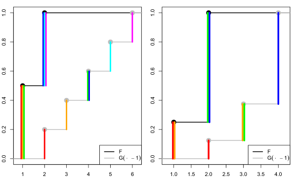
   Figure 2: Visualization of Example 3.10a) in the left panel and of Example 3.10b) in the right panel. The pairs of jumps, of which the heights are to be compared (and which are therefore connected by the relation $\leftrightharpoons$), are marked with the same colour.

2. Because of the simple structure of the cdf’s in part a), they are not instructive for exploring the connection of the relation $\leftrightharpoons$ to the discrete dispersion order $\leq_{\text{disp}}^{\text{disc}}$ given in Proposition 3.8. Therefore, we also consider the following pair of cdf’s. Let $X\sim F$ and $Y\sim G$ be defined by

   $$\mathbb{P}(X=1) =\tfrac{1}{4},\quad \mathbb{P}(X=2) = \;\tfrac{3}{4}$$ ,

   $$\mathbb{P}(Y=1) =\tfrac{1}{8},\quad \mathbb{P}(Y=2) = \;\tfrac{1}{4} ,\quad\mathbb{P}(Y=3)=\tfrac{5}{8}.$$

   Note that $F$ and $G$ are cdf’s of lattice distributions with distance one between neighbouring points in the support; therefore, condition (2) is satisfied. Once again, the indexing sets $A$ and $B$ of $F$ and $G$ are given by their supports. As mentioned ahead of Example 3.10, the sets $(0,1)\setminus F(D_{F})$ and $(0,1)\setminus G(D_{G})$ are disjoint unions of intervals of the form $(F(x_{a-1}),F(x_{a})),a\in A,$ and $(G(y_{b-1}),G(y_{b})),b\in B$, respectively. Specifically,

   $$(0,1)\setminus F(D_{F}) =(0,\tfrac{1}{4})\cup(\tfrac{1}{4},1),$$

   $$(0,1)\setminus G(D_{G}) =(0,\tfrac{1}{8})\cup(\tfrac{1}{8},\tfrac{3}{8})\cup(\tfrac{3}{8},1).$$

   By considering whether the pairwise intersections of these intervals are empty or not, we obtain

   $$R(\leftrightharpoons)=\{(1,1),(1,2),(2,2),(2,3)\}$$

   (see right panel of Figure 2). Going back to the definition of $F$ and $G$, it is obvious that the first jump of $F$ is at least as high as the first two jumps of $G$ and the second jump of $F$ is higher than the last two jumps of $G$. By Proposition 3.8, this yields $F\leq_{\text{disp}}^{\text{disc}}G$. Note that the third jump of $G$ (height $\frac{5}{8}$) is higher than the first jump of $F$ (height $\frac{1}{4}$), represented by the pair $(1,3)\in A\times B$ of indices. However, because the jumps do not overlap, $(1,3)\notin R(\leftrightharpoons)$, i.e. the comparison is not relevant to the discrete dispersion order.

Example 3.10b) shows that requirement (4) of the order $\leq_{\text{disp}}^{\text{disc}}$ compares the jump heights of the two involved distributions pointwise as opposed to uniformly. The original dispersion order $\leq_{\text{disp}}$ also compares in an pointwise manner as it just compares the gradient of the quantile functions at every point in the unit interval. The comparison of the gradient of $F^{-1}$ at one point to the gradient of $G^{-1}$ at another point is irrelevant. The meaning of pointwise comparisons is less obvious in a discrete setting, but as explained above, two jumps are to be compared if they overlap. As mentioned in Example 3.10a), this occurs, if and only if a point connecting the two jumps is part of the Q-Q-plot, which means that the two points share a common piece of probability mass among them. This is different from a uniform comparison since there are pairs of jumps, whose comparison is irrelevant, just like in the continuous setting.

3.2 Comparing the lengths of constant intervals

With the very restrictive requirement (2), the discrete order $\leq_{\text{disp}}^{\text{disc}}$ seems to work fine. However, without this requirement, the order is not sufficient to capture all relevant aspects of dispersion. Specifically, the requirement (4) only looks at the distribution of the probability mass on the respective support, but not at the structure of that support, which explains the nature of the additional requirement (2). A simple example, in which (4) alone is not sufficient, is Example 3.4a), where $F$ and $G$ are two non-tied empirical distribution functions of the same sample size. There, the pmf’s of both distributions are constantly equal on their respective supports and therefore, the difference in dispersion depends solely on the structure of the support.

Now, we want to obtain a weaker dispersion order than $\leq_{\text{disp}}^{\text{disc}}$ for arbitrary cdf’s $F,G\in\mathcal{D}_{0}$ by maintaining the condition (4) for how the probability mass is distributed on the support and weakening the condition (2) for how the support is structured. The first condition, i.e.

$$g(G^{-1}(r))\leq f(F^{-1}(r))\quad\forall r\in(0,1),$$

can be applied to pairs of cdf’s not satisfying condition (2). In the general setting, the condition is still well-defined and meaningful. While this is also true for condition (2), it is not pointwise, but uniform in nature. A pointwise requirement on the supports of $F,G\in\mathcal{D}_{0}$ is given in the equivalent characterization of $F\leq_{\text{disp}}G$ in Proposition 3.3 by

$$\lambda^{1}(F^{-1}(\{r\}))\leq\lambda^{1}(G^{-1}(\{r\}))\quad\forall r\in F(D_{F}).$$ (6)

This, however, is not a reasonable condition, if the additional requirement $F(D_{F})\subseteq G(D_{G})$ is not satisfied. To this end, assume that there exists an $r_{0}\in F(D_{F})\setminus G(D_{G})$ and that (6) holds. This yields

$$0<\lambda^{1}(F^{-1}(\{r_{0}\}))\leq\lambda^{1}(G^{-1}(\{r_{0}\}))=0,$$

a contradiction. Thus, a modification of condition (6) for arbitrary cdf’s $F,G\in\mathcal{D}_{0}$ is needed. If the ranges of $F$ and $G$ do not satisfy $F(D_{F})\subseteq G(D_{G})$, it is reasonable to once again utilize the relation $\leftrightharpoons$ as an indicator for which comparisons are relevant. The subject of the comparison is (in (6) as well as in (2)) the distance, over which the cdf’s takes one specific value. So the condition is given by

$$x_{a}-x_{a-1}\leq y_{b}-y_{b-1}$$

for whichever pairs $(a,b)\in A\times B$ of indices are to be compared, but generally not for all possible pairs. However, since we compare the constant intervals between two jumps and $\leftrightharpoons$ relates two jumps to each other, requiring the comparison for all $(a,b)\in R(\leftrightharpoons)$ results in some unreasonable asymmetries. This is exemplified and visualized in the following.

Example 3.11.

1. Let $F,G\in\mathcal{D}_{0}$. Furthermore, let $A=\{1,2,3\}$, $B=\{1,2,3,4\}$ and let $p_{j}=\tfrac{1}{3}$ for all $j\in A$ and $q_{j}=\tfrac{1}{4}$ for all $j\in B$. The set $R(\leftrightharpoons)$ is given by

   $$R(\leftrightharpoons)=\{(1,1),(1,2),(2,2),(2,3),(3,3),(3,4)\}=\bigcup_{a\in A}\{(a,a),(a,a+1)\}.$$

   For the given cdf’s, we have $\min A=\min B=1$, implying $x_{0}=y_{0}=-\infty$. Since the quantities to be compared are $x_{a}-x_{a-1}$ and $y_{b}-y_{b-1}$, this leads to a problem in the case that either $a$ or $b$ are equal to $1$. Then, both of the above quantities are infinite and graphically, we would not compare the length of a constant interval between two jumps but rather the length of the constant interval before all jumps. Since this is not a sensible procedure, we instead require

   $$x_{a}-x_{a-1}\leq y_{b}-y_{b-1}\quad\forall(a,b)\in R(\leftrightharpoons)\cap\left((A\setminus\{\min A\})\times(B\setminus\{\min B\})\right).$$ (7)

   The remaining pairs of indices to be compared are $(2,2)$, $(2,3)$, $(3,3)$ and $(3,4)$. Similarly to Example 3.10, the constant intervals to be compared are illustrated in the left panel of Figure 3 along with the cdf’s. In this example, this seems to be a reasonable choice.

   

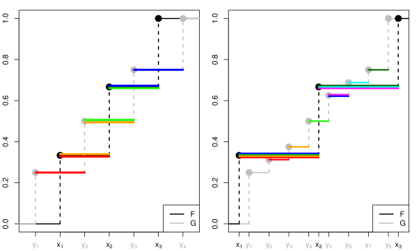
   Figure 3: Visualization of Example 3.11a) in the left panel and of Example 3.11b) in the right panel. The pairs of constant intervals, of which the lengths are deemed to be compared by $\leftrightharpoons$, are marked with the same colour.

2. Let $F$ be defined as in part a) and let $G\in\mathcal{D}_{0}$ be defined by $B=\{1,\ldots,{8}\}$ and

   $$(q_{1},\ldots,q_{8})^{\top}=\frac{1}{16}\left(4,1,1,2,2,1,1,4\right)^{\top},$$

   yielding

   $$F(D_{F})=\left\{\frac{1}{3},\frac{2}{3}\right\},\quad G(D_{G})=\left\{\frac{4}{16},\frac{5}{16},\frac{6}{16},\frac{8}{16},\frac{10}{16},\frac{11}{16},\frac{12}{16}\right\}.$$

   Considering $\frac{5}{16}<\frac{1}{3}<\frac{6}{16}$ and $\frac{10}{16}<\frac{2}{3}<\frac{11}{16}$, we obtain

   $$R(\leftrightharpoons)=\{(1,1),(1,2),(1,3),(2,3),(2,4),(2,5),(2,6),(3,6),(3,7),(3,8)\}.$$

   Once again, we disregard the first three pairs for the comparisons of the constant intervals. The comparisons of the remaining pairs are illustrated in the right panel of Figure 3. Here, it becomes apparent that the relation $\leftrightharpoons$ alone is not fit to decide which pairs of constant intervals are to be compared with respect to their lengths. In spite of the obvious symmetry of both $F$ and $G$, their comparison is highly asymmetric. This is evidenced by the pairs of indices $(2,2),(3,8)\in(A\setminus\{\min A\})\times(B\setminus\{\min B\})$, which are symmetric, but satisfy $(3,8)\in R(\leftrightharpoons)\not\ni(2,2)$. An analogous statement is true for the pairs $(3,3),(2,5)$ and the pairs $(2,4),(3,4)$.

In Example 3.11b), the constant interval of $F$ we identified with the index $a\in A\setminus\{\min A\}$ had the length $x_{a}-x_{a-1}$ and is the interval between the $(a-1)$-th and the $a$-th jump of the cdf. Therefore, it is just as reasonable to identify this interval with the index $a-1\in A\setminus\{\max A\}$ instead of $a$. So, an alternative method of comparing the lengths of the pairs of constant intervals of $F$ and $G$ would be

$$x_{a+1}-x_{a}\leq y_{b+1}-y_{b}\quad\forall(a,b)\in R(\leftrightharpoons)\cap\left((A\setminus\{\max A\})\times(B\setminus\{\max B\})\right).$$ (8)

The resulting illustration for this type of comparison in Example 3.11a) is the same as in the left panel of Figure 3. However, the asymmetries in the resulting illustration for Example 3.11b) are reversed.

It can be shown that the comparisons via (7) and via (8) both yield asymmetric results in a perfectly mirrored way. An evident strategy for obtaining a symmetric comparison is to combine the two methods in such a way that the asymmetries cancel out. There are two intuitive possibilities for this combination. They can either be combined via a logical and ($\land$) or via a logical or ($\lor$). In the following, both possibilities are explored. We start by defining two new relations that indicate the pairs of constant intervals to be compared for both proposed methods. For any indexing set $A\in\mathbb{I}$, we introduce the short hands $\underline{A}=A\setminus\{\min A\}$, $\overline{A}=A\setminus\{\max A\}$ and $\overline{\underline{A}}=A\setminus\{\min A,\max A\}$.

Definition 3.12.

Let $F,G\in\mathcal{D}_{0}$.

1. The relation $\stackrel{{\scriptstyle{\scriptscriptstyle{F},{G}}}}{{\leftrightharpoons_{\land}}}$ on the set $\underline{A}\times\underline{B}$ is defined by

   $$a\stackrel{{\scriptstyle{\scriptscriptstyle{F},{G}}}}{{\leftrightharpoons_{\land}}}b\Leftrightarrow(a\stackrel{{\scriptstyle{\scriptscriptstyle{F},{G}}}}{{\leftrightharpoons}}b)\land(a-1\stackrel{{\scriptstyle{\scriptscriptstyle{F},{G}}}}{{\leftrightharpoons}}b-1)$$

   for $a\in\underline{A},b\in\underline{B}$. The set $R(\stackrel{{\scriptstyle{\scriptscriptstyle{F},{G}}}}{{\leftrightharpoons_{\land}}})$ of all $(a,b)\in\underline{A}\times\underline{B}$ with $a\stackrel{{\scriptstyle{\scriptscriptstyle{F},{G}}}}{{\leftrightharpoons_{\land}}}b$ is said to be the set of $(F,G)$-$\land$-dispersion-relevant pairs of indices.

2. The relation $\stackrel{{\scriptstyle{\scriptscriptstyle{F},{G}}}}{{\leftrightharpoons_{\lor}}}$ on the set $\underline{A}\times\underline{B}$ is defined by

   $$a\stackrel{{\scriptstyle{\scriptscriptstyle{F},{G}}}}{{\leftrightharpoons_{\lor}}}b\Leftrightarrow(a\stackrel{{\scriptstyle{\scriptscriptstyle{F},{G}}}}{{\leftrightharpoons}}b)\lor(a-1\stackrel{{\scriptstyle{\scriptscriptstyle{F},{G}}}}{{\leftrightharpoons}}b-1)$$

   for $a\in\underline{A},b\in\underline{B}$. The set $R(\stackrel{{\scriptstyle{\scriptscriptstyle{F},{G}}}}{{\leftrightharpoons_{\lor}}})$ of all $(a,b)\in\underline{A}\times\underline{B}$ with $a\stackrel{{\scriptstyle{\scriptscriptstyle{F},{G}}}}{{\leftrightharpoons_{\lor}}}b$ is said to be the set of $(F,G)$-$\lor$-dispersion-relevant pairs of indices.

Definition 3.13.

Let $F,G\in\mathcal{D}_{0}$.

1. $G$ is said to be at least as discretely dispersed as $F$ with respect to the probability mass, denoted by $F\leq_{\text{D-pm}}^{\text{disc}}G$, if

   $$q_{b}\leq p_{a}\quad\forall(a,b)\in R(\leftrightharpoons).$$

2. $G$ is said to be at least as $\land$-discretely dispersed as $F$ with respect to the support, denoted by $F\leq_{\text{D-supp}}^{\land\text{-disc}}G$, if

   $$x_{a}-x_{a-1}\leq y_{b}-y_{b-1}\quad\forall(a,b)\in R(\leftrightharpoons_{\land}).$$

   If $F\leq_{\text{D-pm}}^{\text{disc}}G$ and $F\leq_{\text{D-supp}}^{\land\text{-disc}}G$ hold, $G$ is said to be at least as $\land$-discretely dispersed as $F$, denoted by $F\leq_{\text{disp}}^{\land\text{-disc}}G$.

3. $G$ is said to be at least as $\lor$-discretely dispersed as $F$ with respect to the support, denoted by $F\leq_{\text{D-supp}}^{\lor\text{-disc}}G$, if

   $$x_{a}-x_{a-1}\leq y_{b}-y_{b-1}\quad\forall(a,b)\in R(\leftrightharpoons_{\lor}).$$

   If $F\leq_{\text{D-pm}}^{\text{disc}}G$ and $F\leq_{\text{D-supp}}^{\lor\text{-disc}}G$ hold, $G$ is said to be at least as $\lor$-discretely dispersed as $F$, denoted by $F\leq_{\text{disp}}^{\lor\text{-disc}}G$.

Obviously, the orders $\leq_{\text{D-pm}}^{\text{disc}}$ and $\leq_{\text{D-supp}}^{\land\text{-disc}}$ are a kind of split of the $\land$-discrete dispersive order, where the first ordering acts with respect to the y-axis or the probability mass and the second ordering with respect to the x-axis or the support of the distribution. The same split holds for the $\lor$-discrete dispersive order. Since $a\leftrightharpoons_{\lor}b$ implies $a\leftrightharpoons_{\land}b$ for all $(a,b)\in\underline{A}\times\underline{B}$, we have $R(\leftrightharpoons_{\land})\subseteq R(\leftrightharpoons_{\lor})$. By Definition 3.13, this yields

$$F\leq_{\text{disp}}^{\lor\text{-disc}}G\Longrightarrow F\leq_{\text{disp}}^{\land\text{-disc}}G$$

for all $F,G\in\mathcal{D}_{0}$, i.e. $\leq_{\text{disp}}^{\land\text{-disc}}$ is a weakening of $\leq_{\text{disp}}^{\lor\text{-disc}}$. Next, the performance of both orders is examined using the cdf’s from Example 3.11.

Example 3.14 (Continuation of Example 3.11).

1. Consider the cdf’s $F$ and $G$ as defined in Example 3.11a). Based on the set $R(\leftrightharpoons)$, it follows that

   $$R(\leftrightharpoons_{\land})=R(\leftrightharpoons_{\lor})=\{(2,2),(2,3),(3,3),(3,4)\}=R(\leftrightharpoons)\cap(\underline{A}\times\underline{B}).$$

   Hence, all four discussed discrete dispersion orders with respect to the support ($\leq_{\text{D-supp}}^{\land\text{-disc}}$, $\leq_{\text{D-supp}}^{\lor\text{-disc}}$, (7), and (8)) yield the same result for this simple example.

   Since the pmf’s of $F$ and $G$ are both constant on their supports, we obviously have $F\leq_{\text{D-pm}}^{\text{disc}}G$. Hence, the validity of $F\leq_{\text{disp}}^{\land\text{-disc}}G$ and $F\leq_{\text{disp}}^{\lor\text{-disc}}G$ depends solely on four conditions concerning the vectors $(x_{1},x_{2},x_{3})$ and $(y_{1},y_{2},y_{3},y_{4})$, since $|R(\leftrightharpoons_{\land})|=|R(\leftrightharpoons_{\lor})|=4$. To be exact,

   $$F\leq_{\text{disp}}^{\land\text{-disc}}G\Leftrightarrow F\leq_{\text{disp}}^{\lor\text{-disc}}G \Leftrightarrow \;x_{2}-x_{1} \leq y_{2}-y_{1},\ x_{2}-x_{1}\; \leq \;y_{3}-y_{2},$$

   $$\;x_{3}-x_{2} \leq y_{3}-y_{2},\ x_{3}-x_{2}\; \leq \;y_{4}-y_{3}.$$

2. Consider the cdf’s $F$ and $G$ as defined in Example 3.11b). From the set $R(\leftrightharpoons)$ given in that example, we infer

   $$R(\leftrightharpoons_{\land}) =\{(2,3),(2,4),(3,6),(3,7)\},$$

   $$R(\leftrightharpoons_{\lor}) =\{(2,2),(2,3),(2,4),(3,4),(2,5),(3,5),(2,6),(3,6),(3,7),(3,8)\}.$$

   

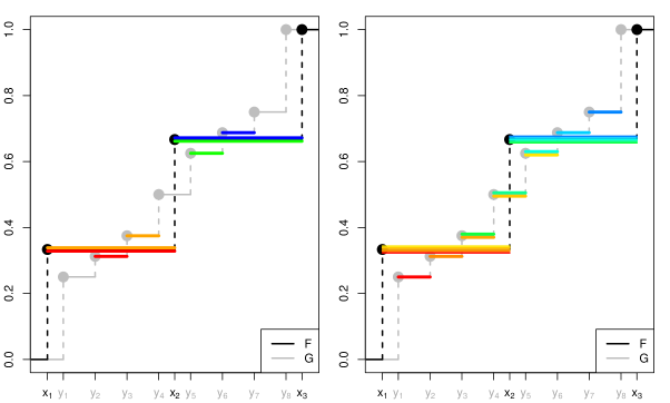
   Figure 4: Visualization of Example 3.14b). The pairs of constant intervals, of which the lengths are to be compared with respect to $\leftrightharpoons_{\land}$ (in the left panel) and $\leftrightharpoons_{\lor}$ (in the right panel), are marked with the same colour.

   The difference in the number of comparisons dictated by $\leftrightharpoons_{\land}$ ($|R(\leftrightharpoons_{\land})|=4$) and $\leftrightharpoons_{\lor}$ ($|R(\leftrightharpoons_{\lor})|=10$) is quite large. Examining the structure of both sets suggests that there is a connection between $|R(\leftrightharpoons_{\land})|$, i.e. the number of $\land$-comparisons, and $|\underline{A}|$, i.e. the cardinal number of the indexing set of $F$, the candidate for the less dispersed cdf. For each element in the latter set, there are two elements in the former set. As depicted in the left panel of Figure 4, the length of every constant interval of $F$ is compared with the lengths of the two closest constant intervals of $G$, one from above and one from below. Since, in this example, $\underline{B}$ is much larger than $\underline{A}$, the constant intervals of $G$ connected to the indices $2,5,8\in\underline{B}$ are not used for any comparison. Hence, the statement $F\leq_{\text{disp}}^{\land\text{-disc}}G$ is completely independent from their lengths. One might say that the pointwise nature of the comparison via $\leq_{\text{D-supp}}^{\land\text{-disc}}$ is dictated by $F$.

   A similar connection can be observed between $|R(\leftrightharpoons_{\lor})|$ and $|\underline{B}|$, i.e. the cardinal number of the indexing set of $G$, the candidate for the more dispersed cdf. Graphically, this means that every constant interval of $G$ is compared with the lengths of the closest constant intervals of $F$ from above and below, provided that the respective intervals exist. Hence, the pointwise comparison via $\leq_{\text{D-supp}}^{\lor\text{-disc}}$ seems to be dictated by $G$.

The idea that the pointwise comparisons of $\leq_{\text{disp}}^{\land\text{-disc}}$ are dictated by the candidate for the less dispersed cdf $F$ and that the pointwise comparisons of $\leq_{\text{disp}}^{\lor\text{-disc}}$ are dictated by the candidate for the more dispersed cdf $G$ are formalized and generalized in the following. Preliminarily, we define the set of (upper and lower) nearest neighbours and prove a helpful lemma.

Definition 3.15.

Let $F,G\in\mathcal{D}_{0}$ and let $a\in\underline{A}$. Then, the set of (upper and lower) nearest neighbours of $F$ in $G$ with respect to $a$ (denoted by $\operatorname{NN}_{F}^{G}(a)$) is defined as follows.

1. If $G(D_{G})\cap(0,F(x_{a-1})]\neq\emptyset$ and $G(D_{G})\cap[F(x_{a-1}),1)\neq\emptyset$, define

   $$\operatorname{NN}_{F}^{G}(a)=\left\{\sup\left(G(D_{G})\cap(0,F(x_{a-1})]\right),\inf\left(G(D_{G})\cap[F(x_{a-1}),1)\right)\right\}.$$

2. If $G(D_{G})\cap(0,F(x_{a-1})]=\emptyset$ and $G(D_{G})\cap[F(x_{a-1}),1)\neq\emptyset$, define

   $$\operatorname{NN}_{F}^{G}(a)=\left\{\inf\left(G(D_{G})\cap[F(x_{a-1}),1)\right)\right\}.$$

3. If $G(D_{G})\cap(0,F(x_{a-1})]\neq\emptyset$ and $G(D_{G})\cap[F(x_{a-1}),1)=\emptyset$, define

   $$\operatorname{NN}_{F}^{G}(a)=\left\{\sup\left(G(D_{G})\cap(0,F(x_{a-1})]\right)\right\}.$$

Here, it is impossible that both sets are empty since this would imply $\emptyset=G(D_{G})\cap(0,1)=G(D_{G})$ and thus $|\operatorname{supp}(G)|=1$, which contradicts $G\in\mathcal{D}_{0}$. Furthermore, note that $F(x_{a-1})$ is the value that $F$ takes on the interval $[x_{a-1},x_{a})$, which is generally associated with the index $a$.

Lemma 3.16.

Let $F,G\in\mathcal{D}_{0}$ satisfy $F\leq_{\text{D-pm}}^{\text{disc}}G$.

1. Let $a\in A$. Then, exactly one of the following two statements holds:

   1. $\exists b\in\overline{B}:F(x_{a-1})<G(y_{b})<F(x_{a})$,

   2. $\exists b\in B:F(x_{a-1})=G(y_{b-1})$ and $F(x_{a})=G(y_{b})$.

2. For all $a\in\overline{A}$, there exist $b_{1},b_{2}\in\overline{B}$ such that $G(y_{b_{1}})\leq F(x_{a})\leq G(y_{b_{2}})$ holds.

The following chain of inequalities follows directly from Lemma 3.16:

$$\inf G(D_{G})\leq\inf F(D_{F})\leq\sup F(D_{F})\leq\sup G(D_{G}).$$

Proposition 3.17.

Let $F,G\in\mathcal{D}_{0}$ satisfy $F\leq_{\text{D-pm}}^{\text{disc}}G$. Then,

1. $R(\leftrightharpoons_{\land})=\bigcup_{a\in\underline{A}}\left(\{a\}\times\{\beta\in\underline{B}:G(y_{\beta-1})\in\operatorname{NN}_{F}^{G}(a)\}\right)$,

2. $R(\leftrightharpoons_{\lor})=\bigcup_{b\in\underline{B}}\left(\{\alpha\in\underline{A}:F(x_{\alpha-1})\in\operatorname{NN}_{G}^{F}(b)\}\times\{b\}\right)$.

Proposition 3.17 confirms the conjecture made in Example 3.14b) to be true. Specifically, $\leftrightharpoons_{\land}$ combines all constant intervals of $F$ with the nearest neighbouring intervals of $G$ and $\leftrightharpoons_{\lor}$ does so the other way around. Since Lemma 3.16 states that $G(D_{G})$ partitions the interval $(0,1)$ in a finer way than $F(D_{F})$, this also provides a heuristic explanation of why $\leq_{\text{D-supp}}^{\land\text{-disc}}$ is a weakening of $\leq_{\text{D-supp}}^{\lor\text{-disc}}$ (and thus $\leq_{\text{disp}}^{\land\text{-disc}}$ is a weakening of $\leq_{\text{disp}}^{\lor\text{-disc}}$).

We have now derived two candidates for a discrete dispersive order in $\leq_{\text{disp}}^{\land\text{-disc}}$ and $\leq_{\text{disp}}^{\lor\text{-disc}}$. Their properties and compatibility with well-known discrete distributions and dispersion measures as well as subsequent indications of advantages and disadvantages of the two candidates are analyzed throughout the remainder of this paper.

Note that the derived orders are not dependend upon the specific utilized definition of quantiles. For $p\in(0,1)$, valid definitions of the $p$-quantile of a cdf $F$ are given by all values in the interval $[\inf\{t\in\mathbb{R}:F(t)\geq p\},\sup\{t\in\mathbb{R}:F(t)\leq p\}]$. It can easily be verified that all of these definitions yield the same candidates for discrete disperive orders.

4 Properties of the discrete dispersive orders

4.1 Crucial properties

The most obvious property that a discrete generalization of the dispersive order should have is its equivalence to the original dispersive order $\leq_{\text{disp}}$ on their joint area of applicability, so if $F(D_{F})\subseteq G(D_{G})$ holds. As shown in the following result, this is only true for one of the two discrete orders derived in Section 3.

Theorem 4.1.

If $F,G\in\mathcal{D}_{0}$ satisfy $F(D_{F})\subseteq G(D_{G})$, then the following implication and equivalence hold:

$$F\leq_{\text{disp}}^{\lor\text{-disc}}G\Longrightarrow F\leq_{\text{disp}}^{\land\text{-disc}}G\Longleftrightarrow F\leq_{\text{disp}}G.$$

Note that the implication in Theorem 4.1 is strict, i.e. that the reverse implication $F\leq_{\text{disp}}^{\land\text{-disc}}G\Rightarrow F\leq_{\text{disp}}^{\lor\text{-disc}}G$ does not hold in general under the assumption $F(D_{F})\subseteq G(D_{G})$. A counterexample is obtained by considering $X\sim\mbox{Bin}(1,\frac{1}{2})$ and $\mathbb{P}(Y=0)=\frac{1}{2}$, $\mathbb{P}(Y=1)=\frac{1}{4}$ and $\mathbb{P}(Y=\frac{3}{2})=\frac{1}{4}$.

The remaining crucial properties to be considered are crucial for all orders underlying essential distributional characteristics like location, dispersion or skewness. Stochastic orders of this kind are, strictly speaking, preorders or quasiorders. This means that they are reflexive and transitive relations, but they are neither antisymmetric nor total. Totality would mean that each pair of distributions is ordered in one of the two possible directions. This does not make sense since the stochastic order is a foundation underneath measures of the same distributional characteristic. Thus, two distributions should only be ordered if the difference between them is beyond any doubt; if the decision is not unambiguous, it is left up to the measure that is built on the foundation of the order. Antisymmetry would mean that the order being valid in both directions would imply that the two distributions are the same. In the case of dispersion orders, this does not make sense since two distributions that only differ by a shift are still considered equivalent with respect to dispersion.

This leaves us with reflexivity and transitivity as crucial properties for foundational stochastic orders and they have been treated as such in the literature [14, see, e.g.,]. Reflexivity is an important property since it reinforces that the considered order is weak and not strict in nature, i.e. that $\leq$ is the correct symbol as opposed to $<$. Transitivity is even more important because it ensures that the order is a suitable foundation for corresponding measures. Since measures assign real numbers to distributions, their values are compared using the transitive relation ‘$\leq$’. If the underlying stochastic order does not share this transitivity, the results can be fatal, as exemplified for orders and measures of kurtosis in [8].

The discrete dispersive orders are analyzed with respect to reflexivity and transitivity in the following result.

Theorem 4.2.

Let $F,G,H\in\mathcal{D}_{0}$.

1. The orders $\leq_{\text{disp}}^{\land\text{-disc}}$ and $\leq_{\text{disp}}^{\lor\text{-disc}}$ are both reflexive, i.e. $F\leq_{\text{disp}}^{\land\text{-disc}}F$ and $F\leq_{\text{disp}}^{\lor\text{-disc}}F$.

2. The order $\leq_{\text{disp}}^{\lor\text{-disc}}$ is transitive, i.e. $F\leq_{\text{disp}}^{\lor\text{-disc}}G$ and $G\leq_{\text{disp}}^{\lor\text{-disc}}H$ implies $F\leq_{\text{disp}}^{\lor\text{-disc}}H$. However, in general, the order $\leq_{\text{disp}}^{\land\text{-disc}}$ is not transitive.

It turns out that both proposed discrete dispersion orders satisfy all except one of the crucial properties. $\leq_{\text{disp}}^{\lor\text{-disc}}$ is transitive but strictly stronger than the original dispersive order on their joint area of applicability. $\leq_{\text{disp}}^{\land\text{-disc}}$ is equivalent to $\leq_{\text{disp}}$ on that area but is not transitive. This begs the question whether there even exists a discrete dispersion order that satisfies both properties. While this question cannot be answered rigorously here, a heuristic explanation suggesting that such an order does not exist is given following the proof of Theorem 4.2.

A notable exception to this problem is given by the class of all lattice distributions.

Corollary 4.3.

1. Let $F$ and $G$ be cdf’s of lattice distributions with distances $c_{F},c_{G}>0$ between neighbouring support points. Then, the following equivalences hold:

   $$F\leq_{\text{disp}}^{\lor\text{-disc}}G\Leftrightarrow F\leq_{\text{disp}}^{\land\text{-disc}}G\Leftrightarrow F\leq_{\text{disp}}^{\text{disc}}G\Leftrightarrow F\leq_{\text{D-pm}}^{\text{disc}}G\ \text{ and }\ c_{F}\leq c_{G}.$$

2. The orders $\leq_{\text{disp}}^{\text{disc}}$, $\leq_{\text{disp}}^{\land\text{-disc}}$ and $\leq_{\text{disp}}^{\lor\text{-disc}}$ are transitive on the set of all lattice distributions.

Corollary 4.3 shows that the limitations of our approach to define a discrete dispersive order are not relevant for lattice distributions, which is one of the two most important classes of discrete distributions; the other one being the class of empirical distributions. First, one does not have to choose one of the two given options for discrete dispersive orders because they coincide. And second, the one remaining discrete dispersive order fulfils all cricial properties stated throughout this subsection.

4.2 Further properties

In this subsection, we further legitimize $\leq_{\text{disp}}^{\land\text{-disc}}$ and $\leq_{\text{disp}}^{\land\text{-disc}}$ as discrete versions of the dispersive order $\leq_{\text{disp}}$ by proving that a number of positive results concerning $\leq_{\text{disp}}$ are also true for the discrete orders. First, we consider the equivalence classes of the relation $=_{\text{disp}}$, which denotes equivalence with respect to the order $\leq_{\text{disp}}$. Note that $=_{\text{disp}}$ inherits the properties of reflexivity and transitivity from $\leq_{\text{disp}}$, and it is symmetric by definition. Thus, $=_{\text{disp}}$ is an equivalence relation. The equivalence class of any $F\in\mathcal{D}_{0}$ with respect to $=_{\text{disp}}$ is given by all real shifts of $F$, i.e. $\{F(\cdot-\lambda):\lambda\in\mathbb{R}\}$ [14, see], so distributions that are equivalent with respect to dispersion can only differ in location. The following are the discrete versions of that result.

Theorem 4.4.

Let $F,G\in\mathcal{D}_{0}$. Then, the following three statements are equivalent:

1. $F=_{\text{disp}}^{\land\text{-disc}}G$,

2. $F=_{\text{disp}}^{\lor\text{-disc}}G$,

3. there exists a $\lambda\in\mathbb{R}$ such that $G(t)=F(t-\lambda)$ for all $t\in\mathbb{R}$.

Theorem 4.4 particularly states that $F=_{\text{disp}}^{\land\text{-disc}}G$ is equivalent to $F=_{\text{disp}}^{\lor\text{-disc}}G$ for all $F,G\in\mathcal{D}_{0}$. Since $=_{\text{disp}}^{\lor\text{-disc}}$ inherits reflexivity and transitivity as its properties from $\leq_{\text{disp}}^{\lor\text{-disc}}$ and is obviously symmetric, it is an equivalence relation. Its equivalence classes are, as for $\leq_{\text{disp}}$, of the form $\{F(\cdot-\lambda):\lambda\in\mathbb{R}\}$ for $F\in\mathcal{D}_{0}$. We can now consider the quotient set of $\mathcal{D}_{0}$ by $=_{\text{disp}}^{\lor\text{-disc}}$, denoted by $\mathcal{D}_{0}/=_{\text{disp}}^{\lor\text{-disc}}$, and also define both discrete dispersion orders on that set. For all $\mathcal{F},\mathcal{G}\in\mathcal{D}_{0}/=_{\text{disp}}^{\lor\text{-disc}}$, the orders are defined by

$$\mathcal{F}\leq_{\text{disp}}^{\lor\text{-disc}}\mathcal{G},\quad\text{if and only if}\quad\exists F\in\mathcal{F},G\in\mathcal{G}:F\leq_{\text{disp}}^{\lor\text{-disc}}G,$$

and analogously for $\leq_{\text{disp}}^{\land\text{-disc}}$. The consideration of these equivalence classes is relevant to the following result.

Proposition 4.5.

Let $F,G\in\mathcal{D}_{0}$ not belong to the same equivalence class of $\mathcal{D}_{0}$ by $=_{\text{disp}}^{\land\text{-disc}}$. Then, it follows from $F\leq_{\text{disp}}^{\land\text{-disc}}G$ that either $\lambda^{1}(D_{F})=\lambda^{1}(D_{G})=\infty$ or $\lambda^{1}(D_{F})<\lambda^{1}(D_{G})$ holds. The same is true for $\leq_{\text{disp}}^{\lor\text{-disc}}$ in place of $\leq_{\text{disp}}^{\land\text{-disc}}$.

An analogous result also holds for the the original dispersive order. It directly follows from its Definition 2.2a) and from $\lambda^{1}(D_{F})=\lim_{\alpha\searrow 0}(F^{-1}(1-\alpha)-F^{-1}(\alpha))$, $\lambda^{1}(D_{G})=\lim_{\alpha\searrow 0}(G^{-1}(1-\alpha)-G^{-1}(\alpha))$.

Another result that relates the dispersive order to the supports of the involved distributions is given in [13, p. 42, Theorem 1.7.6a) ] and can also be reproduced for both discrete dispersive orders.

Proposition 4.6.

Let $F,G\in\mathcal{D}_{0}$. If $F\leq_{\text{disp}}^{\land\text{-disc}}G$ and $\min(\operatorname{supp}(F))\leq\min(\operatorname{supp}(G))$ with both minimums existing, then $F\leq_{\text{st}}G$. The same is true for $\leq_{\text{disp}}^{\lor\text{-disc}}$ in place of $\leq_{\text{disp}}^{\land\text{-disc}}$.

Analogously, if $F$ is less dispersed than $G$ with respect to either order, and $\max(\operatorname{supp}(F))\geq\max(\operatorname{supp}(G))$ holds with both maximums existing, $F\leq_{\text{st}}G$ also follows.

4.3 Relationships to other orders of dispersion

Analyzing the relationship to other dispersion orders is not only helpful in terms of integrating the discrete dispersive orders into an existing framework, but also simplifies the proof of whether certain dispersion measures preserve the discrete dispersive orders. For example, since the standard deviation is centered around the mean, just like the dilation order, it is much easier to show that the standard deviation preserves the dilation order than to show the analogous statement directly for the dispersive order.

Before coming to the dilation order as the most well-known alternative dispersion order toward the end of this subsection, we start out with another order of dispersion that is related to the usual stochastic order. The so-called weak dispersive order was introduced and noted to be weaker than $\leq_{\text{disp}}$ by [9, p. 326 ], who used it as a starting point for a multivariate dispersion order. They said that $F$ precedes $G$ in the weak dispersive order, if $|X-X^{\prime}|\leq_{\text{st}}|Y-Y^{\prime}|$ holds for $X,X^{\prime}\sim F$ independent and $Y,Y^{\prime}\sim G$ independent.

Theorem 4.7.

Let $F,G\in\mathcal{D}_{0}$ with $X,X^{\prime}\sim F$ independent and $Y,Y^{\prime}\sim G$ independent. Then, $F\leq_{\text{disp}}^{\land\text{-disc}}G$ implies $|X-X^{\prime}|\leq_{\text{st}}|Y-Y^{\prime}|$.

Obviously, it follows directly that $\leq_{\text{disp}}^{\lor\text{-disc}}$ is also stronger than the weak dispersive order.

In order to see that the reverse implication of Theorem 4.7 is not true, we make use of the fact that $\leq_{\text{disp}}^{\land\text{-disc}}$ is not transitive. For that, let $F,G,H\in\mathcal{D}_{0}$ be defined as in the part of the proof of Theorem 4.2b), where the counterexample for the transitivity of $\leq_{\text{disp}}^{\land\text{-disc}}$ was constructed. It is shown there that $F\leq_{\text{disp}}^{\land\text{-disc}}G$ and $G\leq_{\text{disp}}^{\land\text{-disc}}H$, but $F\not\leq_{\text{disp}}^{\land\text{-disc}}H$. If we now let $X,X^{\prime}\sim F$ independent, $Y,Y^{\prime}\sim G$ independent and $Z,Z^{\prime}\sim H$ independent, Theorem 4.7 yields $|X-X^{\prime}|\leq_{\text{st}}|Y-Y^{\prime}|$ as well as $|Y-Y^{\prime}|\leq_{\text{st}}|Z-Z^{\prime}|$. Since the stochastic order is transitive, we have now shown $|X-X^{\prime}|\leq_{\text{st}}|Z-Z^{\prime}|$ while $F\not\leq_{\text{disp}}^{\land\text{-disc}}H$ holds and, thus, that the statement of Theorem 4.7 is indeed a strict implication.

We now turn our attention to the dilation order $\leq_{\text{dil}}$, which is a weakening of the original dispersive order $\leq_{\text{disp}}$ (see Proposition 2.3b)). The proof of this implication given by [14, pp. 158–159 ] employs a third order as an intermediate step. This intermediate order is denoted by $\leq_{1}^{*}$ by [14] and $F\leq_{1}^{*}G$ is said to hold, if, under the assumption of equal means, the cdf’s $F$ and $G$ intersect exactly once with $F$ being smaller than $G$ before the intersection and larger afterwards.

The fact that the discrete dispersive orders also imply the dilation order is proved in a similar way. However, the intersection criterion in this case is not as simple as for $\leq_{\text{disp}}$. The following lemma gives the corresponding result, which is the discrete analogue of $\leq_{1}^{*}$.

Lemma 4.8.

Let $F,G\in\mathcal{D}_{0}$ with $F\neq G$ have finite and coinciding means and satisfy $F\leq_{\text{disp}}^{\land\text{-disc}}G$. Then:

1. $\exists(a,b)\in A\times\underline{B}:F(x_{a-1})\leq G(y_{b-1})\leq F(x_{a}),y_{b-1}<x_{a}\leq y_{b}$.

2. One of the following two statements is true:

   1. $\exists(a,b)\in\overline{A}\times\overline{B}:F(x_{a})=G(y_{b}),y_{b}<x_{a},x_{a+1}\leq y_{b+1}$   or

   2. $\exists(a,b)\in A\times\underline{B}:F(x_{a-1})<G(y_{b-1})<F(x_{a}),y_{b-1}<x_{a}\leq y_{b}$.

As mentioned before, the statement of Lemma 4.8 is the discrete analogue of an intersection of $F$ and $G$ in the continuous case, which is the transition from $G$ being larger to $F$ being larger. Note that part b) is just a more refined version of part a) and distinguishes between two kinds of intersection equivalents, both of which are depicted schematically in Figure 5.

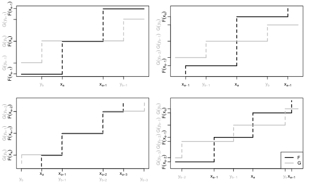
Figure 5: Different variations of ’generalized intersections’ between two standardized (w.r.t. the mean) cdf’s $F$ and $G$ with $F\leq_{\text{disp}}^{\land\text{-disc}}G$, as specified in Lemma 4.8b). Left panels: condition (i). Right panels: condition (ii).

If condition (i) is fulfilled, the images of the two (standardized) cdf’s share a common element and the generalized intersection occurs as both cdf take that value. This means that (the more dispersed cdf) $G$ is larger than $F$ before said constant interval. After the constant interval, $G$ is either smaller than $F$ right away (as in the upper left panel of Figure 5) or the two cdf’s coincide for a while before $G$ eventually becomes smaller (as in the lower left panel). The specific formulation of condition (i) (and also condition (ii)) that allows equality on the right side but not on the left is somewhat arbitrary in the sense that one could swap the requirements without invalidating the result. Although this potentially results in a different pair $(a,b)$ indicating at which point the intersection takes place, that pair could be used in the same way going forward. Note that if equality was disallowed on both sides, Lemma 4.8 would no longer be true.

If condition (ii) is fulfilled, a jump of $F$ and a constant interval of $G$ form a cross (or a kind of degenerated cross if equality holds on the right side as discussed in the previous paragraph). $G$ is either larger than $F$ before that cross and smaller after (as exemplified in the upper right panel of Figure 5) or this kind of situation can occur repeatedly (as exemplified in the lower right panel). The latter situation is the main difficulty in the proof of the following theorem.

Theorem 4.9.

Let $F,G\in\mathcal{D}_{0}$ have finite means. Then, $F\leq_{\text{disp}}^{\land\text{-disc}}G$ implies $F\leq_{\text{dil}}G$.

According to Theorems 4.7 and 4.9 and, to a lesser extent, Lemma 4.8, the discrete dispersive orders relate to other orders of dispersion for discrete distributions in the same way as the original dispersive order does for continuous distributions.

5 Discrete dispersion measures

In this section, we consider a number of well-known measures of dispersion in the classical sense of Definition 2.1 and analyze their compatibility with the discrete dispersion orders derived in Section 3. If a measure preserves these orders, it reliably and meaningfully measures not only the dispersion of continuous distributions, but also of discrete distributions. However, if a measure does not preserve either discrete dispersive order, this presents a rigorous argument for discouraging the use of this dispersion measure on discrete distributions.

First, the considered dispersion measures are introduced along with refrences for their fulfilment of properties (D1) and (D2) from Definition 2.1. Most of the references only prove (D2) since (D1) is obtained easily by utilising basic properties of the mean, quantiles and expectiles.

Proposition 5.1.

For $F\in\mathcal{P}$, let $X,X^{\prime}\sim F$ be independent and let $e_{X}:(0,1)\to\mathbb{R}$ be the corresponding expectile function in the case $F\in\mathcal{L}^{1}$.

1. The standard deviation

   $$\mathrm{SD}:\mathcal{L}^{2}\to[0,\infty),\quad F\mapsto\sqrt{\mathbb{E}[(X-\mathbb{E}[X])^{2}]}$$

   satisfies conditions (D1) and (D2), see [14, p. 159 ].

2. The Gini mean difference

   $$\mathrm{GMD}:\mathcal{L}^{1}\to[0,\infty),\quad F\mapsto\mathbb{E}[|X-X^{\prime}|]$$

   satisfies conditions (D1) and (D2), see [14, p. 160 ].

3. The mean absolute deviation from the mean

   $$\mathrm{MAD}:\mathcal{L}^{1}\to[0,\infty),\quad F\mapsto\mathbb{E}[|X-\mathbb{E}[X]|]$$

   satisfies conditions (D1) and (D2), see [10, p. 15 ].

4. The mean absolute deviation from the median

   $$\mathrm{MDMAD}:\mathcal{L}^{1}\to[0,\infty),\quad F\mapsto\mathbb{E}[|X-F^{-1}(\tfrac{1}{2})|]$$

   satisfies conditions (D1) and (D2), see [10, p. 15 ].

5. For $0<\alpha<\beta<1$, the $(\alpha,\beta)$-interquantile range

   $$\mathrm{IQR}({\alpha},{\beta}):\mathcal{P}\to[0,\infty),\quad F\mapsto F^{-1}(\beta)-F^{-1}(\alpha)$$

   satisfies conditions (D1) and (D2) by definition.

6. For $0<\alpha<\tfrac{1}{2}<\beta<1$, the $(\alpha,\beta)$-interexpectile range

   $$\mathrm{IER}({\alpha},{\beta}):\mathcal{L}^{1}\to[0,\infty),\quad F\mapsto e_{X}(\beta)-e_{X}(\alpha)$$

   satisfies conditions (D1) and (D2), see [7, p. 517 ].

The measures $\mathrm{IQR}({\alpha},{\beta})$ and $\mathrm{MDMAD}$ involving quantiles require minor assumptions to satisfy (D1) in a discrete setting. It is sufficient to assume that the involved cdf is strictly increasing in the points at which the quantile function is evaluated. These additional assumptions are not necessary, if the alternative definition of the quantile $F^{-1}(p),p\in(0,1),$ given by

$$\tfrac{1}{2}\big{(}\inf\{t\in\mathbb{R}:F(t)\geq p\}+\sup\{t\in\mathbb{R}:F(t)\leq p\}\big{)}$$

is utilized, which is often done for empirical quantiles.

The fact that most of the measures from Definition 5.1 preserve $\leq_{\text{disp}}^{\land\text{-disc}}$ follows directly from Theorems 4.7 and 4.9.

Corollary 5.2.

The mappings $\mathrm{SD}$, $\mathrm{MAD}$ and $\mathrm{GMD}$ all preserve the order $\leq_{\text{disp}}^{\land\text{-disc}}$.

For $\mathrm{SD}$ and $\mathrm{MAD}$, this follows from Theorem 4.9 since both $t\mapsto t^{2}$ and $t\mapsto|t|$ are convex functions on the real numbers. For $\mathrm{GMD}$, it follows from Theorem 4.7 since the expected value is a measure of (central) location, which preserves the usual stochastic order $\leq_{\text{st}}$. We can also use Theorem 4.9 to show that $\mathrm{GMD}$ preserves $\leq_{\text{disp}}^{\land\text{-disc}}$ since $F\leq_{\text{dil}}G$ implies $\mathrm{GMD}(F)\leq\mathrm{GMD}(G)$, as proved in [15, p. 126, Thm. 2.2 ] and pointed out by [16, p. 65 ]. Conversely, the fact that $\mathrm{SD}$ preserves $\leq_{\text{disp}}^{\land\text{-disc}}$ also follows from Theorem 4.7 because of

$$\mathrm{SD}(F)^{2}=\mathbb{E}[X^{2}]-\mathbb{E}[X]^{2}=\tfrac{1}{2}\left(\mathbb{E}[X^{2}]-2\mathbb{E}[X]\mathbb{E}[X^{\prime}]+\mathbb{E}[{X^{\prime}}^{2}]\right)=\tfrac{1}{2}\mathbb{E}[(X-X^{\prime})^{2}]$$

for $X,X^{\prime}\sim F$ independent.

It can be shown in a similar way that $\mathrm{IER}({\alpha},{\beta})$ preserves the order $\leq_{\text{disp}}^{\land\text{-disc}}$ for $0<\alpha<\frac{1}{2}<\beta<1$, which includes all cases relevant for applications. This again holds due to Theorem 4.9, combined with the fact that $F\leq_{\text{dil}}G$ implies $\mathrm{IER}({\alpha},{\beta})(F)\leq\mathrm{IER}({\alpha},{\beta})(G)$ for all $0<\alpha<\frac{1}{2}<\beta<1$. This implication was first shown by [1, p. 2020, Thm. 3(b) ]; a more elementary proof that also includes the reverse implication is given by [7, p. 517 ]. The assumptions can be weakened to include all distributions in $\mathcal{D}_{0}\cap\mathcal{L}^{1}$ without changing the proof.

Corollary 5.3.

If $0<\alpha<\frac{1}{2}<\beta<1$, the mapping $\mathrm{IER}({\alpha},{\beta})$ preserves the order $\leq_{\text{disp}}^{\land\text{-disc}}$.

It remains to be determined whether the mappings $\mathrm{IQR}({\alpha},{\beta})$ and $\mathrm{MDMAD}$ preserve $\leq_{\text{disp}}^{\land\text{-disc}}$. Both mappings are based on quantiles, which are well-known to be not as useful for discrete as for continuous distributions. This is partly due to the fact that they are not unique in the discrete case. Furthermore, quantiles only evaluate a distribution in a very local sense, which also explains their popularity in robust statistics. However, for discrete distributions, where the probability mass is very sparse, this leads to a lack of information that is conveyed by single evaluations of quantile functions. In accordance with these observations, the interquantile range $\mathrm{IQR}({\alpha},{\beta})$ does generally not preserve the discrete dispersive orders, as noted in the following result.

Theorem 5.4.

For all choices $0<\alpha<\beta<1$, the mapping $\mathrm{IQR}({\alpha},{\beta})$ does not preserve the order $\leq_{\text{disp}}^{\land\text{-disc}}$.

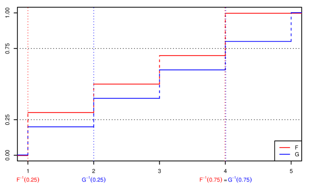
Figure 6: Illustration of a counterexample for Theorem 5.4 with $\alpha=\frac{1}{4}$, $\beta=\frac{3}{4}$.

The statement of Theorem 5.4 also holds, if we replace $\leq_{\text{disp}}^{\land\text{-disc}}$ by $\leq_{\text{disp}}^{\lor\text{-disc}}$ or even $\leq_{\text{disp}}^{\text{disc}}$. This is due to the fact that the distributions used in the proof of Theorem 5.4 are lattice distributions, for which all discrete dispersive orders are equivalent (see Corollary 4.3a)).

A counterexample for the interquartile range $\mathrm{IQR}({\frac{1}{4}},{\frac{3}{4}})$ is depicted in Figure 6. The cdf $F$ is specified by by $\mathbb{P}(X=1)=\mathbb{P}(X=4)=\frac{3}{10}$ and $\mathbb{P}(X=2)=\mathbb{P}(X=3)=\frac{1}{5}$ while $G$ is specified by $Y\sim\mathcal{U}(\{1,\ldots,5\})$. Heuristically, to obtain $G$, a third of the probability mass on the outer two jumps of $F$ is shifted outwards and the two pieces are combined to obtain an additional jump. In accordance with this heuristic explanation, it is easy to show that $F\leq_{\text{disp}}^{\land\text{-disc}}G$ holds since all jump heights of $G$ are smaller than all jump heights of $F$. In particular, $F$ is strictly less dispersed because its support is a subset of the support of $G$. However, Figure 6 clearly shows that the interquartile range of $G$ is smaller than that of $F$, meaning that the measure is obviously misrepresenting their relationship with respect to dispersion. In applied sciences, where dispersion measures are trusted to be meaningful, this could lead to severe misinterpretations of the data.

Only one of the two drawbacks of using quantile-based measures on discrete distributions is actually relevant for the failure of the interquantile range. Just like in the counterexample depicted in Figure 6, all quantiles used for the proof of Theorem 5.4 are unique. Thus, the result is also valid for all alternative definitions of quantiles. The failure of the interquantile range is due to the merely local evaluation of the involved distributions, which is not suitable for the sparse nature of discrete distributions. This incompatibility is particularly serious for distributions with small supports.

Theorem 5.4 implies that the interquantile range is not fit to be used as a dispersion measure for discrete distributions. This statement is similar to [2, p. 1852 ] suggesting that the interquantile range is not a ‘true measure of variability’ because it does not preserve the dilation order. However, it is obvious from the definition of the original dispersive order $\leq_{\text{disp}}$ that the interquantile range indeed measures dispersion in a meaningful way for continuous distributions. The requirement that dispersion measures should preserve the dilation order is simply too strong. Neither the interquantile range nor the mean absolute deviation from the median could be proved to meet this requirement.

The fact that $\mathrm{MDMAD}$ preserves the order $\leq_{\text{disp}}^{\land\text{-disc}}$ cannot be established as a simple corollary as for all other positive results in this section. In particular, $F\leq_{\text{disp}}^{\land\text{-disc}}G$ does not generally imply $|X-F^{-1}(\frac{1}{2})|\leq_{\text{st}}|Y-G^{-1}(\frac{1}{2})|$; a counterexample is given by

$$\mathbb{P}(X=0) = \frac{1}{2},\ \mathbb{P}(X=1) =\mathbb{P}(X=2)\; = \;\frac{1}{4},$$

$$\mathbb{P}(Y=0) = \frac{3}{8},\ \mathbb{P}(Y=1) =\mathbb{P}(Y=2)\; = \;\frac{1}{4},\ \mathbb{P}(Y=3)=\frac{1}{8}.$$

However, the implication still holds, as shown in the following.

Theorem 5.5.

The mapping $\mathrm{MDMAD}$ preserves the order $\leq_{\text{disp}}^{\land\text{-disc}}$.

6 Behaviour of discrete distributions in the new framework

In this section, we analyze whether popular families of discrete distributions preserve the discrete dispersive orders. Since all of the distributions considered in the following are lattice distributions with defining distance equal to one, all previously defined discrete dispersive orders are equivalent and it is sufficient to consider the order $\leq_{\text{D-pm}}^{\text{disc}}$ (see Corollary 4.3a)). In the formulation of the results, the order $\leq_{\text{disp}}^{\land\text{-disc}}$ is used since it is the discrete order that is closest to $\leq_{\text{disp}}$. The only considered non-lattice distribution is the discrete uniform distribution on arbitrary finite sets, which is discussed at the end of the following subsection.

6.1 Discrete uniform and empirical distribution

The discrete uniform distribution is the simplest discrete distribution. In its usual variant, it puts the same amount of probability mass on a finite number of points that are equidistantly spaced with distance $1$. Since all of the dispersion orders and measures considered in the previous chapters are location invariant, it is sufficient to consider uniform distributions with supports $\{1,\ldots,n\},n\in\mathbb{N}_{\geq 2}$. If $\mathbb{P}(X=k)=\frac{1}{n}$ for all $k\in\{1,\ldots,n\}$, we denote this by $X\sim\mathcal{U}[n]$. These distributions are also used in Example 2.5 in order to establish that the original dispersive order is far from sufficient for discrete distributions. However, it is easy to show that any two discrete uniform distributions are ordered with respect to the discrete dispersive orders introduced in this work.

Proposition 6.1.

Let $n,m\in\mathbb{N}_{\geq 2},n<m,$ and let $X\sim\mathcal{U}[n]$ and $Y\sim\mathcal{U}[m]$. Then, $X\leq_{\text{disp}}^{\land\text{-disc}}Y$ holds.

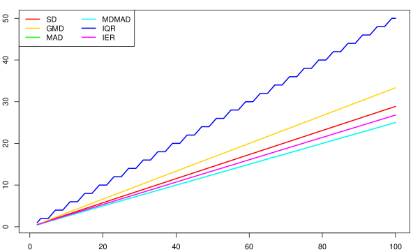
Figure 7: Plot of $\tau(X)$ for six different dispersion measures $\tau$ and $X\sim\mathcal{U}[n]$, as a function of $n\in\{2,\ldots,100\}$. The measures $\mathrm{MAD}$ and $\mathrm{MDMAD}$ coincide here because of symmetry.

The behaviour of the dispersion measures from Section 5 for discrete uniform distributions as a function of the parameter $n$ is depicted in Figure 7. It shows that five of the six dispersion measures are almost linearly increasing as a function of $n$, although the slight deviations from linearity can barely be seen in Figure 7. The average slopes differ between the measures; only $\mathrm{MAD}$ and $\mathrm{MDMAD}$ are exactly the same since the distribution is symmetric. The graph of the interquartile range $\mathrm{IQR}$ has a different shape since it only takes values in the natural numbers when applied to a lattice distribution with defining distance $1$. This lack of granularity is also somewhat indicative of its lack of compatibility with discrete distributions that is formalized in Theorem 5.4. However, a counterexample for the proof of Theorem 5.4 cannot be constructed using this class of discrete uniform distributions.

The concept of discrete uniform distributions can be generalized to arbitrary finite sets. Let $S\subset\mathbb{R}$ with $|S|=n\in\mathbb{N}_{\geq 2}$. If now $\mathbb{P}(X=s)=\frac{1}{n}$ for any $s\in S$, then $X$ is discretely uniformly distributed on $S$, denoted by $X\sim\mathcal{U}(S)$. Note that the set of all generalized discrete uniform distributions is equal to the set of all non-tied empirical distributions. Because of the complexity of this family of distributions, we refrain from trying to obtain general results with respect to discrete dispersive orders. Instead, we discuss a number of special cases for the order $\leq_{\text{disp}}^{\land\text{-disc}}$ in the following example.

Example 6.2.

Let $S,T\subset\mathbb{R}$ with $2\leq|S|=m<n=|T|$ and let $X\sim\mathcal{U}(S)$, $Y\sim\mathcal{U}(T)$.

1. Let $n$ be a multiple of $m$, so there exists a $c\in\mathbb{N}_{\geq 2}$ such that $n=c\cdot m$. Because of

   $$F(D_{F}) =\{\tfrac{k}{m}:k\in\{1,\ldots,{m-1}\}\}=\{\tfrac{c\cdot k}{n}:k\in\{1,\ldots,{m-1}\}\}$$

   $$\subset\{\tfrac{k}{n}:k\in\{1,\ldots,{n-1}\}\}=G(D_{G}),$$

   $F\leq_{\text{disp}}^{\land\text{-disc}}G$ is equivalent to $F\leq_{\text{disp}}G$ in this case. According to Proposition 3.3, $F\leq_{\text{disp}}^{\land\text{-disc}}G$ holds if $x_{k+1}-x_{k}\leq y_{c\cdot k+1}-y_{c\cdot k}$ holds for all $k\in\{1,\ldots,{m-1}\}$. Hence, $m-1$ comparisons are made overall, one per constant interval of $F$.

2. Let $n$ be a multiple of $m$ plus one, so there exists a $c\in\mathbb{N}$ such that $n=c\cdot m+1$. It follows that $m$ and $n$ are coprime and $F(D_{F})\cap G(D_{G})=\emptyset$. Furthermore, for each $k\in\{1,\ldots,{m-1}\}$, it holds that $\frac{k}{m}=\frac{c\cdot k}{n-1}\in(\frac{c\cdot k}{n},\frac{c\cdot k+1}{n})$. Hence, $\operatorname{NN}_{F}^{G}(k+1)=\{\tfrac{c\cdot k}{n},\tfrac{c\cdot k+1}{n}\}$ for all $k\in\{1,\ldots,{m-1}\}$. Since $F\leq_{\text{D-pm}}^{\text{disc}}G$ is obviously satisfied, Proposition 3.17a) states that $F\leq_{\text{disp}}^{\land\text{-disc}}G$ is equivalent to

   $$x_{k+1}-x_{k} \leq y_{c\cdot k+1}-y_{c\cdot k}\quad\text{and}$$

   $$x_{k+1}-x_{k} \leq y_{c\cdot k+2}-y_{c\cdot k+1}$$

   for all $k\in\{1,\ldots,{m-1}\}$. Hence, $2m-2$ comparisons are made overall, two per constant interval of $F$.

3. Let the greatest common divisor $d$ of $m$ and $n$ satisfy $1<d<m$, so there exist $c_{F},c_{G}\in\mathbb{N}_{\geq 2}$ such that $m=c_{F}\cdot d$ and $n=c_{G}\cdot d$. Then, $F(D_{F})\cap G(D_{G})=\{\frac{k}{d}:k\in\{1,\ldots,{d-1}\}\}$ since

   $$F(D_{F})\ni\frac{k\cdot c_{F}}{m}=\frac{k\cdot c_{F}}{c_{F}\cdot d}=\frac{k}{d}=\frac{k\cdot c_{G}}{c_{G}\cdot d}=\frac{k\cdot c_{G}}{n}\in G(D_{G})$$

   holds for all $k\in\{1,\ldots,{d-1}\}$ and because $c_{F}$ and $c_{G}$ are coprime by assumption. It follows that $|\operatorname{NN}_{F}^{G}(\ell+1)|=1$, if $\ell$ is a multiple of $c_{F}$, and $|\operatorname{NN}_{F}^{G}(\ell+1)|=2$ otherwise. In the former case, the corresponding comparisons (by Proposition 3.17a)) have the same structure as in part a), and in the latter case they have the same structure as in part b). Overall, there are $2m-2-(d-1)=(2c_{F}-1)d-3$ comparisons to be made. Note that the edge cases $d=m$ and $d=1$ give the situation in part a) and part b), respectively.

6.2 Geometric distribution

Except for the discrete uniform distribution, the geometric distribution is the only popular type of discrete distribution with an explicit representation of the cdf. We use the following version of the geometric distribution: if $X\sim\mathrm{Geom}(\pi)$ with $\pi\in(0,1)$, then $\mathbb{P}(X=k)=\pi\cdot(1-\pi)^{k-1}$ for $k\in\mathbb{N}$. The cdf of $X$ is then given by $F(t)=1-(1-\pi)^{\lfloor t\rfloor}$ for $t\geq 0$. Graphically, the dispersion of the distribution seems to decrease as the parameter $\pi$ increases. Furthermore, for $F=\mathrm{Geom}(\pi_{F})$ and $G=\mathrm{Geom}(\pi_{G})$ with $0<\pi_{G}<\pi_{F}<1$, $F\leq_{\text{st}}G$ and even $F<_{st}G$ obviously holds, which already implies $G\not\leq_{\text{disp}}^{\land\text{-disc}}F$ according to Proposition 4.6. The following result gives a sufficient condition for the ordering of two geometric distributions with respect to $\leq_{\text{disp}}^{\land\text{-disc}}$.

Theorem 6.3.

Let $X\sim\mathrm{Geom}(\pi_{F})$ and $Y\sim\mathrm{Geom}(\pi_{G})$ with $0<\pi_{G}<\pi_{F}<1$ have cdf’s $F$ and $G$. If

$$(\pi_{F},\pi_{G})\in\left\{(1-\lambda^{\varrho},1-\lambda):\frac{1}{2}<\lambda<1,\varrho\geq\frac{\log(2\lambda-1)}{\log(\lambda)}-1\right\},$$

then $F\leq_{\text{disp}}^{\land\text{-disc}}G$ holds.

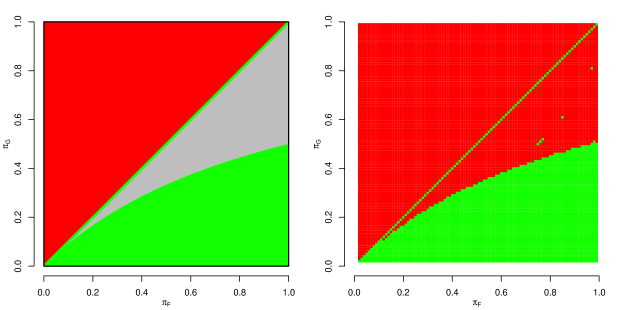
Figure 8: Plot of theoretical (left panel) and numerical (right panel) results concerning $F\leq_{\text{disp}}^{\land\text{-disc}}G$ for all possible parameter choices $\pi_{F},\pi_{G}\in(0,1)$ for $F=\mathrm{Geom}(\pi_{F})$ and $G=\mathrm{Geom}(\pi_{G})$. In green areas, $F\leq_{\text{disp}}^{\land\text{-disc}}G$ holds; in red areas, $F\not\leq_{\text{disp}}^{\land\text{-disc}}G$ holds; in grey areas, no result could be obtained.

The set of parameter pairs from Theorem 6.3 is visualized in the left panel of Figure 8, where it is the green area on the lower right. The grey area represents those combinations of parameters, for which no theoretical result could be obtained. In order to determine the behaviour in these grey areas, a numerical analysis was conducted. Since the support of the geometric distribution is infinite, the cdf’s and pdf’s were cut off at $10^{6}$. The results with $0.01$ as increment for the parameters $\pi_{F}$ and $\pi_{G}$ are depicted in the right panel of Figure 8. The numerical results look almost identical to the theoretical results with the grey area filled in red. It is not clear whether the few sparse green dots in that area actually represent $F\leq_{\text{disp}}^{\land\text{-disc}}G$ holding or they represent numerical inaccuracies. Either way, the numerical results suggest that the implication in Theorem 6.3 is close to being an equivalence as the number of counterexamples for the reverse implication is very small.

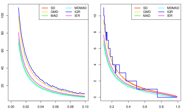
Figure 9: Plot of $\tau(X)$ for six different dispersion measures $\tau$ and $X\sim\mathrm{Geom}(\pi)$, as a function of $\pi\in(0,1)$. Note the different scales in the two panels.

The behaviour of the dispersion measures from Section 5 applied to geometric distributions is shown in Figure 9. First, it is obvious that the graphs all have similar shapes. While that includes the interquartile range $\mathrm{IQR}$ to a certain degree, its graph is the only one that is not decreasing on the entire parameter space. Furthermore, the slopes of all graphs decrease significantly for increasing parameter values. Thus, there is a smaller difference in dispersion between two similarly high values of $\pi$ than there is between two similarly low values of $\pi$. This observation is in agreement with the behaviour of the discrete dispersion order for geometric distributions. Consider the following example: according to Theorem 6.3 and Figure 8, $F\leq_{\text{disp}}^{\land\text{-disc}}G$ holds for $\pi_{F}=0.15$ and $\pi_{G}=0.12$ while $F\not\leq_{\text{disp}}^{\land\text{-disc}}G$ holds for $\pi_{F}=0.9$ and $\pi_{G}=0.72$, which differ from each other by the same factor.

6.3 Binomial distribution

The binomial distribution has two parameters to be varied, namely the sample size $n$ and the success probability $\pi$. However, if we consider two distributions $F=\mathrm{Bin}(n,\pi_{F})$ and $G=\mathrm{Bin}(n,\pi_{G})$ with $n\in\mathbb{N}_{\geq 2}$ and $\pi_{F},\pi_{G}\in(0,1),\pi_{F}\neq\pi_{G}$, Proposition 4.5 states that neither $F\leq_{\text{disp}}^{\land\text{-disc}}G$ nor $G\leq_{\text{disp}}^{\land\text{-disc}}F$ holds. That is because of $D_{F}=D_{G}=[0,n)$, which yields $\lambda^{1}(D_{F})=\lambda^{1}(D_{G})=n<\infty$. Heuristically, the binomial distribution seems to be most dispersed when it is symmetric. Its dispersion declines, if the success probability becomes markedly high or low as then, the probability mass is concentrated heavily on one side. This observation is reflected in the left panel of Figure 10, which depicts the behaviour of the dispersion measures from Chapter 5 for fixed $n$ and varying $\pi$.

Furthermore, the plot shows that the dispersion measures display differing degrees of smoothness as a function of the success probability. While $\mathrm{IQR}$ is the only measure that is not continuous, $\mathrm{MAD}$, $\mathrm{MDMAD}$ and $\mathrm{IER}$ also exhibit some lack of smoothness. Solely the graphs of $\mathrm{SD}$ and $\mathrm{GMD}$ look like they could stem from an infinitely often differentiable function.

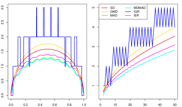
Figure 10: Plot of $\tau(X)$ for six different dispersion measures $\tau$ and $X\sim\mathrm{Bin}(n,\pi)$. Left panel: $n=10$ fixed, $\tau(X)$ as a function of $\pi$. Right panel: $\pi=\frac{1}{2}$ fixed, $\tau(X)$ as a function of $n$.

For binomial distributions with fixed success probability $\pi$ and varying sample size $n$, we restrict ourselves to the symmetric case $\pi=\frac{1}{2}$. If we consider two distributions $F=\mathrm{Bin}(m,\frac{1}{2})$ and $G=\mathrm{Bin}(n,\frac{1}{2})$ with $m,n\in\mathbb{N}_{\geq 2}$ and $m<n$, we can once again invoke Proposition 4.5 to obtain $G\not\leq_{\text{disp}}^{\land\text{-disc}}F$. The remaining question is: if at all, under which conditions concerning $m$ and $n$ does $F\leq_{\text{disp}}^{\land\text{-disc}}G$ hold? Because of the non-explicit structure of the cdf of the binomial distribution, no theoretical result answering this question could be proved. Instead, we have to rely solely on numerical computations.

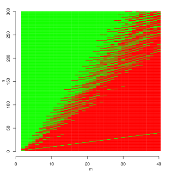
Figure 11: Plot of the numerical results concerning $F\leq_{\text{disp}}^{\land\text{-disc}}G$ for selected parameter values for $F=\mathrm{Bin}(m,\frac{1}{2})$ and $G=\mathrm{Bin}(n,\frac{1}{2})$. In green areas, $F\leq_{\text{disp}}^{\land\text{-disc}}G$ holds; in red areas, $F\not\leq_{\text{disp}}^{\land\text{-disc}}G$ holds. Note the different scales of the two axes.

The results are depicted in Figure 11. They generally support the graphical impression that the (symmetric) binomial distribution becomes more dispersed as its sample size increases. However, the difference between the two sample sizes $m$ and $n$ needs to be quite large for $F\leq_{\text{disp}}^{\land\text{-disc}}G$ to hold. For $n<5m$, $F\leq_{\text{disp}}^{\land\text{-disc}}G$ only holds very sporadically. For $5m\leq n\leq 10m$, $F\leq_{\text{disp}}^{\land\text{-disc}}G$ holds in some cases, depending on the compatibility of the two distributions. However, as $n$ approaches $10m$, the share of positive results seems to increase. Finally, for $n>10m$, $F\leq_{\text{disp}}^{\land\text{-disc}}G$ always holds with very few exceptions if $n\approx 10m$. It is notable that the borders between the red and the mixed area as well as between the mixed and the green area both seem to be approximately linear. According to further numerical evaluations for larger sample sizes, the factors of $5$ and $10$ seem to grow a bit further to approximately $8.5$ and $12$ at $m=400$.

The behaviour of the dispersion measures when applied to symmetric binomial distributions is similar to our previous observations. All graphs of the corresponding plot in the right panel of Figure 10 are increasing, once again with the exception of $\mathrm{IQR}$. Their slopes slightly decrease as $n$ is increasing. Their smoothness properties coincide with our observations from the left panel of Figure 10, where $\pi$ varies instead of $n$.

6.4 Poisson distribution

The last discrete distribution considered in this section is the Poisson distribution. For that, we consider two distributions $F=\mathrm{Pois}(\lambda_{F})$ and $G=\mathrm{Pois}(\lambda_{G})$ with $\lambda_{F},\lambda_{G}>0$. Similarly to the geometric distribution, it is easy to show that $F\leq_{\text{st}}G$ and even $F<_{st}G$ holds, if $\lambda_{F}<\lambda_{G}$. By Proposition 4.6, $G\not\leq_{\text{disp}}^{\land\text{-disc}}F$ follows in that case. Whether $F\leq_{\text{disp}}^{\land\text{-disc}}G$ holds can once again only be analyzed numerically since the cdf of the Poisson distribution also does not have an explicit form.

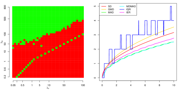
Figure 12: Left panel: Plot of the numerical results concerning $F\leq_{\text{disp}}^{\land\text{-disc}}G$ (green: yes; red: no) for selected parameter values for $F=\mathrm{Pois}(\lambda_{F})$ and $G=\mathrm{Pois}(\lambda_{G})$. Note that the scale on both axes is not linear and only contains exemplary values.
Right panel: Plot of $\tau(X)$ for six different dispersion measures $\tau$ and $X\sim\mathrm{Pois}(\lambda)$, as a function of $\lambda$.

The results for selected values of $\lambda_{F}$ and $\lambda_{G}$ are depicted in the left panel of Figure 12. As for the binomial distribution, $F\leq_{\text{disp}}^{\land\text{-disc}}G$ only seems to hold, if $\lambda_{G}$ is sufficiently large compared to $\lambda_{F}$. However, the differing factor between $\lambda_{F}$ and $\lambda_{G}$ at the border between the red and the green area decreases for increasing $\lambda_{F}$. For $\lambda_{F}=0.05$, that factor is equal to $600$, and it is subsequently reduced: to $70$ for $\lambda_{F}=1$, to $10$ for $\lambda_{F}=10$, and to $5$ for $\lambda_{F}=100$. It is unclear whether this reduction is representative of the actual interaction between the Poisson distribution and the order $\leq_{\text{disp}}^{\land\text{-disc}}$ or it is a numerical phenomenon. The latter explanation is supported by the fact that, with increasing parameter $\lambda$, the amount of probability mass within jumps too small to register numerically also increases. Therefore, more relevant jumps cannot be compared properly.

The behaviour of the dispersion measures plotted in the right panel of Figure 12 is similar to the previous distribution families. The declining slope of the graphs is indicative of smaller differences in dispersion for higher parameter values and therefore suggests that our observations about the left panel are indeed due to numerical inaccuracies.

7 Concluding remarks and future research

The discrete dispersive orders are carefully constructed in Section 3 from the information available about the original dispersive order, particularly about its behaviour on discrete distributions. Still, one could pursue other approaches to define such an order.

One alternative approach could arise out of a small inconsistency of $\leq_{\text{disp}}^{\land\text{-disc}}$, which can be illustrated using Example 3.14. Here, part a) is a limit case of part b) if the lengths of some constant intervals converge to zero. However, the requirements for $\leq_{\text{disp}}^{\land\text{-disc}}$ to hold in the limiting case are quite different to part b). This is due to the fact that, when using $\leq_{\text{disp}}^{\land\text{-disc}}$, some intervals are not part of any comparisons. An alternative approach that solves this is not restricted to comparing single intervals of $F$ to single intervals of $G$, but the lengths of intervals of the more dispersed $G$ that lie between two intervals of $F$ can be combined. More specifically, the length $x_{a}-x_{a-1}$ of each constant interval of $F$ is compared with the cumulated length $\sum_{b\in\underline{B}:p_{a-1}\leq q_{b-1}<p_{a}}(y_{b}-y_{b-1})$ of all constant intervals of $G$ lower than the next constant interval of $F$. $x_{a}-x_{a-1}$ is also be compared with the cumulated length $\sum_{b\in\underline{B}:p_{a-2}<q_{b-1}\leq p_{a-1}}(y_{b}-y_{b-1})$ of constant intervals of $G$ below the interval $[x_{a-1},x_{a})$. This weakens the strong order $\leq_{\text{disp}}^{\land\text{-disc}}$, but seemingly to a small enough degree that the new order is still meaningful. We conjecture that this new order, just like $\leq_{\text{disp}}^{\lor\text{-disc}}$, is transitive, but not equivalent to $\leq_{\text{disp}}$ on their joint area of applicability. Thus, it seems like a suitable order to explore in further work. A downside is that it cannot be described with the relation $\leftrightharpoons$ as intuitively as the other discrete orders. Therefore, it might be difficult or even impossible to replicate some of the results in Sections 4 and 5, while the results in Section 6 are not going to be improved since they only concern lattice distributions.

Another alternative approach is motivated by the fact that, under suitable regularity conditions, $F\leq_{\text{disp}}G$ is equivalent to the slopes of their quantile functions being ordered accordingly in a pointwise sense. Hence, only one quantity needs to be compared instead of the split into jump heights and lengths of constant intervals. The idea would be to interpolate the quantile functions of discrete distributions and to then compare their slopes in a pointwise sense. However, this approach does not seem to be promising. First, the first jumps of the distributions would not be compared in any way. Second, one can find simple examples of counterintuitive behaviour, even disregarding the first problem (e.g., consider $X=\frac{1}{2}\tilde{X}$ with $\tilde{X}\sim\mathrm{Bin}(1,\frac{1}{2})$ and $Y=(1-\varepsilon)\tilde{Y}$ with $\tilde{Y}\sim\mathrm{Bin}(1,1-\varepsilon)$ and let $\varepsilon\searrow 0$). Third, the approach would heavily depend on the specific definition of the quantile function used.

The approach presented throughout this paper has significant upsides: it provides a rigorous foundation underneath discrete dispersion measures that was missing thus far and provides a new, simple and effective way to describe and compare discrete distributions. It is informed by the pointwise and local nature of quantile comparisons and align their evaluations with the sparse occurence of probability mass for discrete distributions. Here, the relation $\leftrightharpoons$ plays a key role. The usual stochastic order can also be described in a simple and straight-forward way using this relation. Furthermore, orders similar to $\leq_{\text{disp}}^{\land\text{-disc}}$ and $\leq_{\text{disp}}^{\lor\text{-disc}}$ can be derived for higher-order distributional characteristics like skewness, which exhibit similar problems as dispersion for discrete distributions [5, see].

Having discussed the merits of this approach based on the relation $\leftrightharpoons$, a number of open questions for future research still remain, mainly concerning the transition of the discrete dispersive orders to the original dispersive order. For example, one could consider a continuous cdf $F$ and approximate it by discrete cdf’s $F_{n}$ such that $F_{n}\stackrel{{\scriptstyle n\to\infty}}{{\to}}F$ in a given mode of convergence. If the same is given for another continuous cdf $G$, a desirable result would be that $F_{n}\leq_{\text{disp}}^{\land\text{-disc}}G_{n}$ for all sufficiently large $n$ implies $F\leq_{\text{disp}}G$. One could also analyze how meaningful the original dispersive order is for mixtures of discrete and continuous distributions and try to suitably bridge that gap if necessary.

Appendix A Proofs

A.1 Proofs for Section 3

Proof of Proposition 3.2.

We define a function $\varphi:\mathcal{D}_{0}\to\bigcup_{A\in\mathbb{I}}\mathbb{S}_{A}$ and show that it is a bijection, which is an even stronger statement than the assertion. Note that the codomain of $\varphi$ is a disjoint union of the sets $\mathbb{S}_{A},A\in\mathbb{I}$. The value assignment of $\varphi$ is now defined by cases. Therefore, let $F\in\mathcal{D}_{0}$, then $\operatorname{supp}(F)$ is order-isomorphic to a subset of $\mathbb{Z}$. Note that since minima and maxima are defined via the order $\leq$, this order-isomorphism preserves minima and maxima.

• $\min(\operatorname{supp}(F))$ and $\max(\operatorname{supp}(F))$ both exist.
  A subset of $\mathbb{Z}$ has a minimum and a maximum, if and only if it is finite. Therefore, $\operatorname{supp}(F)$ is also finite. Let $n=|\operatorname{supp}(F)|\in\mathbb{N}_{\geq 2}$. Define $x_{1}=\min(\operatorname{supp}(F))$ and $x_{j}=\min(\operatorname{supp}(F)\setminus\{x_{1},\ldots,x_{j-1}\}),j=2,\ldots,n$. Then, we define $\varphi(F)=(x_{j},p_{j})_{j\in\{1,\ldots,n\}}\in\mathbb{S}_{\{1,\ldots,n\}}$, where $p_{j}=\mathbb{P}(X=x_{j})>0,j=1,\ldots,n$. Note that all of the steps of the value assignment in this case are unique, thus ensuring injectivity in this case.

• $\min(\operatorname{supp}(F))$ exists, but $\max(\operatorname{supp}(F))$ does not.
  The only set within $\mathbb{I}$ with existing minimum but non-existing maximum is $\mathbb{N}$. Similarly to Case 1, define $x_{1}=\min(\operatorname{supp}(F))$ and $x_{j}=\min(\operatorname{supp}(F)\setminus\{x_{1},\ldots,x_{j-1}\}),j=2,3,\ldots$. Then, the definition $\varphi(F)=(x_{j},p_{j})_{j\in\mathbb{N}}\in\mathbb{S}_{\mathbb{N}}$ with $p_{j}=\mathbb{P}(X=x_{j})>0,j=1,2,\ldots,$ is once again unique.

• $\max(\operatorname{supp}(F))$ exists, but $\min(\operatorname{supp}(F))$ does not.
  This is analogous to Case 2 by simply swapping to roles of minima and maxima and replacing $\mathbb{N}$ by $(-\mathbb{N})$.

• $\min(\operatorname{supp}(F))$ and $\max(\operatorname{supp}(F))$ both do not exist.
  The only set within $\mathbb{I}$ with non-existing minimum and non-existing maximum is $\mathbb{Z}$. We now define

  $$x_{0} =F^{-1}(\tfrac{1}{2})=\inf\{t\in\mathbb{R}:F(t)\geq\tfrac{1}{2}\}\in\operatorname{supp}(F),$$

  $$x_{j} =\min\{t\in\operatorname{supp}(F)\setminus\{x_{0},\ldots,x_{j-1}\}:F(t)\geq\tfrac{1}{2}\},\quad j=1,2,\ldots,$$

  $$x_{j} =\max\{t\in\operatorname{supp}(F)\setminus\{x_{j+1},\ldots,x_{0}\}:F(t)<\tfrac{1}{2}\},\quad j=-1,-2,\ldots.$$

  Defining $\varphi(F)=(x_{j},p_{j})_{j\in\mathbb{Z}}\in\mathbb{S}_{\mathbb{Z}}$ with $p_{j}=\mathbb{P}(X=x_{j})>0,j\in\mathbb{Z},$ now once again leads to a unique value assignment in this case.

It is ensured in every case separately that $\varphi$ is well-defined and injective. Now let $A\in\mathbb{I}$ and $(x_{j},p_{j})_{j\in A}\in\mathbb{S}_{A}$. We define a cdf $F$ by $\mathbb{P}(X=x_{j})=p_{j}>0,j\in A$. It follows directly that $\operatorname{supp}(F)=\{x_{j}:j\in A\}$ is order-isomorphic to $A\subseteq\mathbb{Z}$ with $|A|\geq 2$. This implies $F\in\mathcal{D}_{0}$ and following the above value assignment for $\varphi$ yields $\varphi(F)=(x_{j},p_{j})_{j\in A}$. Thus, $\varphi$ is surjective and therefore a bijection.

Proof of Proposition 3.3.

We start by proving the implication from left to right. Due to Proposition 2.4, only the inequality of the Lebesgue measures needs to be shown. This follows immediately as

$$\lambda^{1}(F^{-1}(\{p\}))=\lim\limits_{r\searrow p}(F^{-1}(r)-F^{-1}(p))\leq\lim\limits_{r\searrow p}(G^{-1}(r)-G^{-1}(p))=\lambda^{1}(G^{-1}(\{p\}))$$ (9)

holds for all $p\in F(D_{F})$ by assumption since $F(D_{F})\subseteq(0,1)$.

For the other implication, let $p,q\in(0,1),p<q$. Since $F$ is discrete, the difference of its quantile function at $p$ and $q$ is equal to the summed lengths of all intervals, on which $F$ is constant at a value between $p$ and $q$. Thus,

$$F^{-1}(q)-F^{-1}(p)=\sum_{r\in F(D_{F})\cap[p,q)}\lambda^{1}(F^{-1}(\{r\}))$$

and analogously for $G$. By assumption, we obtain

$$\ \left(G^{-1}(q)-G^{-1}(p)\right)-\left(F^{-1}(q)-F^{-1}(p)\right)$$

$$= \ \sum_{r\in F(D_{F})\cap[p,q)}\left(\lambda^{1}(G^{-1}(\{r\}))-\lambda^{1}(F^{-1}(\{r\}))\right)+\sum_{r\in\left(G(D_{G})\setminus F(D_{F})\right)\cap[p,q)}\lambda^{1}(G^{-1}(\{r\})).$$

Since both of these summands are non-negative, the assertion follows.

Proof of Proposition 3.8.

The following chain of equivalences proves the assertion:

$$F\leq_{\text{disp}}^{\text{disc}}G \Leftrightarrow g(G^{-1}(r))\leq f(F^{-1}(r))\quad \forall r\in(0,1)$$

$$\Leftrightarrow g(y_{b})\leq f(x_{a})\quad \forall (a,b)\in A\times B\text{ such that}$$

$$F^{-1}(r)=x_{a},G^{-1}(r)=y_{b}\text{ for some }r\in(0,1)$$

$$\Leftrightarrow g(y_{b})\leq f(x_{a})\quad \forall (a,b)\in R(\leftrightharpoons)$$

$$\Leftrightarrow\mathbb{P}(Y=y_{b})\leq\mathbb{P}(X=x_{a})\quad \forall (a,b)\in R(\leftrightharpoons)$$

$$\Leftrightarrow q_{b}\leq p_{a}\quad \forall (a,b)\in R(\leftrightharpoons)$$

The second equivalence holds due to the fact that $\mathrm{range}(F^{-1})=\operatorname{supp}(F)$ and $\mathrm{range}(G^{-1})=\operatorname{supp}(G)$.

Proof of Proposition 3.9.

Let $(a,b)\in A\times B$. Then,

$$F^{-1}(r)=x_{a} \Leftrightarrow r\in(F(x_{a-1}),F(x_{a})],$$

$$G^{-1}(r)=y_{b} \Leftrightarrow r\in(G(y_{b-1}),G(y_{b})].$$

So the existence of an $r\in(0,1)$ such that $F^{-1}(r)=x_{a}$ and $G^{-1}(r)=y_{b}$ is equivalent to the existence of an $r\in(F(x_{a-1}),F(x_{a})]\cap(G(y_{b-1}),G(y_{b})]$. This, in turn, is equivalent to that set being non-empty.

The fact that $(c_{1},c_{2}]\cap(d_{1},d_{2}]\neq\emptyset$ implies $(c_{1},c_{2})\cap(d_{1},d_{2})\neq\emptyset$ for $c_{1},c_{2},d_{1},d_{2}\in\mathbb{R}$ with $c_{1}<c_{2},d_{1}<d_{2}$ concludes the proof.

Proof of Lemma 3.16.

1. We prove the equivalence $\neg(i)\Leftrightarrow(ii)$. Note that $\neg(i)$ is equivalent to $G(D_{G})\cap(F(x_{a-1}),F(x_{a}))=\emptyset$.

   1. It follows that $(F(x_{a-1}),F(x_{a}))\cap G(D_{G})=(G(y_{b-1}),G(y_{b}))\cap G(D_{G})=\emptyset$.

   2. We start by proving that there exists a $b_{u}\in B$ such that $G(y_{b_{u}})\geq F(x_{a})$. If $F(x_{a})<1$, this follows directly from the fact that $\sup G(\operatorname{supp}(G))=1$. If $F(x_{a})=1$, $\sup G(\operatorname{supp}(G))=1$ also implies $\max G(\operatorname{supp}(G))=1$ since, otherwise, $\lim_{\beta\to\infty}G(y_{\beta})-G(y_{\beta-1})=0<1-F(x_{a-1})=F(x_{a})-F(x_{a-1})$ along with $\lim_{\beta\to\infty}G(y_{\beta})=1$ would contradict $F\leq_{\text{D-pm}}^{\text{disc}}G$. Obviously, there also exists a $b_{\ell}\in B\cup\{\min B-1\}$ such that $G(y_{b_{\ell}})\leq F(x_{a-1})$.

      Now, define $b\in B$ by $G(y_{b})=\min(G(\operatorname{supp}(G))\cap[F(x_{a}),1])\leq G(y_{b_{u}})$, yielding $a\leftrightharpoons b$. By assumption $G(y_{b-1})\leq F(x_{a-1})<F(x_{a})\leq G(y_{b})$ holds and it follows that $q_{b}\geq p_{a}$. Equality holds, if and only if $G(y_{b-1})=F(x_{a-1})$ and $G(y_{b})=F(x_{a})$, which corresponds to (ii). If equality does not hold, $F\leq_{\text{D-pm}}^{\text{disc}}G$ is contradicted.

2. Let $a\in\overline{A}$. The assertion follows by applying part a) to both $a$ and $a+1\in A$, and by considering all four arising cases separately.

Proof of Proposition 3.17.

1. First, note that, for all $a\in\underline{A}$, it follows from Lemma 3.16b) that $G(D_{G})\cap(0,F(x_{a-1})]\neq\emptyset$ and $G(D_{G})\cap[F(x_{a-1}),1)\neq\emptyset$. Thus,

   $$\operatorname{NN}_{F}^{G}(a)=\left\{\sup\left(G(D_{G})\cap(0,F(x_{a-1})]\right),\inf\left(G(D_{G})\cap[F(x_{a-1}),1)\right)\right\}.$$

   Because of $\sup G(\operatorname{supp}(G))=1$ and $F(x_{a-1})<1$, there exists a $b\in B$ such that $F(x_{a-1})\in[G(y_{b-1}),G(y_{b}))$. It follows that

   $$\sup(G(D_{G})\cap(0,F(x_{a-1})]) =\max(G(D_{G})\cap(0,F(x_{a-1})])$$

   and, analogously,

   $$\inf(G(D_{G})\cap[F(x_{a-1}),1)) =\min(G(D_{G})\cap[F(x_{a-1}),1)).$$

   1. Let $a\in\underline{A}$. Now $b-1\in\overline{B}$ (or $b\in\underline{B}$) is defined uniquely by $G(y_{b-1})=\max(G(D_{G})\cap(0,F(x_{a-1})])$. If follows that $G(y_{b-1})\leq F(x_{a-1})<G(y_{b})$ and thus, $a\leftrightharpoons b$. The case $G(y_{b-1})=F(x_{a-1})$ is equivalent to

      $$\min(G(D_{G})\cap[F(x_{a-1}),1))=\max(G(D_{G})\cap(0,F(x_{a-1})])=F(x_{a-1}).$$

      Then, there exists an $\varepsilon>0$ such that

      $$(F(x_{a-2}),F(x_{a-1}))\ni F(x_{a-1})-\varepsilon =G(y_{b-1})-\varepsilon\in(G(y_{b-2}),G(y_{b-1})),$$

      $$(F(x_{a-1}),F(x_{a}))\ni F(x_{a-1})+\varepsilon =G(y_{b-1})+\varepsilon\in(G(y_{b-1}),G(y_{b})),$$

      thus yielding $a\leftrightharpoons_{\land}b$. The case $G(y_{b-1})<F(x_{a-1})$ remains to be considered. It immediately follows that $a-1\leftrightharpoons b$. This, combined with $a\leftrightharpoons b$, yields

      $$G(y_{b})-G(y_{b-1})\leq F(x_{a-1})-F(x_{a-2}),\ G(y_{b})-G(y_{b-1})\leq F(x_{a})-F(x_{a-1})$$

      $$\Longrightarrow F(x_{a-2})<G(y_{b-1})<F(x_{a-1})<G(y_{b})<F(x_{a}).$$

      It follows that $a-1\leftrightharpoons b-1$ and $a\leftrightharpoons b+1$, thus, $a\leftrightharpoons_{\land}b$ and $a\leftrightharpoons_{\land}b+1$. Since $G(y_{(b+1)-1})=G(y_{b})=\min(G(D_{G})\cap[F(x_{a-1}),1))$, this concludes the proof of the implication from right to left.

   2. Let $(a,b)\in R(\leftrightharpoons_{\land})\subseteq\underline{A}\times\underline{B}$.

      1. $G(y_{b-1})>F(x_{a-1})$
         Under this assumption, Lemma 3.16 states that $b-1>\min B$. From $a-1\leftrightharpoons b-1$, we then obtain $G(y_{b-2})<F(x_{a-1})$. Consequently, $G(y_{b-1})=\min(G(D_{G})\cap[F(x_{a-1}),1))\in\operatorname{NN}_{F}^{G}(a)$.

      2. $G(y_{b-1})<F(x_{a-1})$
         Similarly to Case 1, we have $a\leftrightharpoons b$, which yields $G(y_{b})>F(x_{a-1})$ and $G(y_{b-1})=\max(G(D_{G})\cap(0,F(x_{a-1})])\in\operatorname{NN}_{F}^{G}(a)$.

      3. $G(y_{b-1})=F(x_{a-1})$
         It immediately follows that

         $$G(y_{b-1}) =\min(G(D_{G})\cap[F(x_{a-1}),1))$$

         $$=\max(G(D_{G})\cap(0,F(x_{a-1})])\in\operatorname{NN}_{F}^{G}(a).$$

2. 1. Let $b\in\underline{B}$. Assume first $F(D_{F})\cap[G(y_{b-1}),1)\neq\emptyset$. Then, with analogous reasoning to part a), there exists an $a\in\underline{A}$ such that

      $$F(x_{a-1})=\inf(F(D_{F})\cap[G(y_{b-1}),1))=\min(F(D_{F})\cap[G(y_{b-1}),1)).$$

      It follows that $F(x_{a-1})\geq G(y_{b-1})>F(x_{a-2})$, where it is possible that $a-1=\min A$ and therefore, $F(x_{a-2})=0$. Nonetheless, we obtain $a-1\leftrightharpoons b-1$ and thus, $a\leftrightharpoons_{\lor}b$.

      Now we assume $F(D_{F})\cap(0,G(y_{b-1})]\neq\emptyset$ (which can occur simultaneously to $F(D_{F})\cap[G(y_{b-1}),1)\neq\emptyset$). Again analogously to part a), there exists an $a\in\underline{A}$ such that

      $$F(x_{a-1})=\sup(F(D_{F})\cap(0,G(y_{b-1})])=\max(F(D_{F})\cap(0,G(y_{b-1})]).$$

      We now infer $F(x_{a-1})\leq G(y_{b-1})<F(x_{a})$, yielding $a\leftrightharpoons b$ and thereby $a\leftrightharpoons_{\lor}b$.

   2. Let $(a,b)\in R(\leftrightharpoons_{\lor})\subseteq\underline{A}\times\underline{B}$.

      1. $F(x_{a-1})<G(y_{b-1})$
         If $a-1\leftrightharpoons b-1$, it follows $G(y_{b-2})<F(x_{a-1})$, which then yields $a\leftrightharpoons b-1$. We obtain

         $$F(x_{a})=F(x_{a-1})+p_{a}\geq F(x_{a-1})+q_{b-1}>G(y_{b-2})+q_{b-1}=G(y_{b-1}).$$

         If $a\leftrightharpoons b$, it follows directly that $F(x_{a})>G(y_{b-1})$. Since $a\leftrightharpoons_{\lor}b$ implies $a\leftrightharpoons b$ or $a-1\leftrightharpoons b-1$, the inequality $F(x_{a})>G(y_{b-1})$ holds generally. It yields $F(x_{a-1})=\max(F(D_{F})\cap(0,G(y_{b-1})])\in\operatorname{NN}_{G}^{F}(b)$.

      2. $F(x_{a-1})>G(y_{b-1})$
         If $a\leftrightharpoons b$, it follows $G(y_{b})>F(x_{a-1})$, which then yields $a-1\leftrightharpoons b$. We obtain

         $$F(x_{a-2})=F(x_{a-1})-p_{a-1}\leq F(x_{a-1})-q_{b}<G(y_{b})-q_{b}=G(y_{b-1}).$$

         If $a-1\leftrightharpoons b-1$, it follows directly that $F(x_{a-2})<G(y_{b-1})$. Thus, the implication $F(x_{a-1})=\min(F(D_{F})\cap[G(y_{b-1}),1))\in\operatorname{NN}_{G}^{F}(b)$ generally holds.

      3. $F(x_{a-1})=G(y_{b-1})$
         Similarly to part a), it immediately follows that

         $$F(x_{a-1}) =\min(F(D_{F})\cap[G(y_{b-1}),1))$$

         $$=\max(F(D_{F})\cap(0,G(y_{b-1})])\in\operatorname{NN}_{G}^{F}(b).$$

A.2 Proofs for Section 4

Proof of Theorem 4.1.

Since the implication holds in a more general setting, only the equivalence must be proven.

We start out by proving that $F(D_{F})\subseteq G(D_{G})$ already implies $F\leq_{\text{D-pm}}^{\text{disc}}G$. To this end, let $(a,b)\in R(\leftrightharpoons)$, i.e.

$$(F(x_{a-1}),F(x_{a}))\cap(G(y_{b-1}),G(y_{b}))\neq\emptyset.$$ (10)

By assumption, $G(y_{b})>F(x_{a})$ implies $F(x_{a})=G(y_{b-1})$ and $G(y_{b-1})<F(x_{a-1})$ implies $F(x_{a-1})=G(y_{b})$, so both cases contradict (10). This yields

$$(G(y_{b-1}),G(y_{b}))\subseteq(F(x_{a-1}),F(x_{a})).$$ (11)

Again by assumption, there exist $b_{u}\in B,b_{\ell}\in B\cup\{-\infty\},b_{\ell}<b_{u}$ such that $F(x_{a})=G(y_{b_{u}})$ and $F(x_{a-1})=G(y_{b_{\ell}})$. By combining this with (11), we obtain $b,b-1\in\{b_{\ell},\ldots,b_{u}\}$ or, equivalently, $b\in\{b_{\ell}+1,\ldots,b_{u}\}$. It follows

$$p_{a}=F(x_{a})-F(x_{a-1})=G(y_{b_{u}})-G(y_{b_{\ell}})=\sum_{j=b_{\ell}+1}^{b_{u}}q_{j}\geq q_{b},$$

thus proving $F\leq_{\text{D-pm}}^{\text{disc}}G$.

It remains to be shown that $F\leq_{\text{disp}}G$ is equivalent to $F\leq_{\text{D-supp}}^{\land\text{-disc}}G$. Note that $F(D_{F})=F(\operatorname{supp}(F))\setminus\{1\}=F(\operatorname{supp}(F)\setminus\{\max(\operatorname{supp}(F))\})$ holds as well as the analogous identity for $G$. The following equivalences hold:

$$F\leq_{\text{disp}}G \Leftrightarrow\lambda^{1}(F^{-1}(\{r\}))\leq\lambda^{1}(G^{-1}(\{r\}))\quad\forall r\in F(D_{F})$$

$$\Leftrightarrow\lambda^{1}(F^{-1}(\{F(x)\}))\leq\lambda^{1}(G^{-1}(\{G(y)\}))$$

$$\hphantom{\Leftrightarrow}\hskip 112.81506pt\forall x\in\operatorname{supp}(F)\setminus\{\max(\operatorname{supp}(F))\},$$

$$\hphantom{\Leftrightarrow}\hskip 112.81506pt\hphantom{\forall}y\in\operatorname{supp}(G)\setminus\{\max(\operatorname{supp}(G))\}:F(x)=G(y)$$

$$\Leftrightarrow\lambda^{1}(F^{-1}(\{F(x_{a})\}))\leq\lambda^{1}(G^{-1}(\{G(y_{b})\}))\ \forall a\in\overline{A},b\in\overline{B}:F(x_{a})=G(y_{b})$$

$$\Leftrightarrow\lambda^{1}([x_{a},x_{a+1}))\leq\lambda^{1}([y_{b},y_{b+1}))\hskip 49.79231pt\forall a\in\overline{A},b\in\overline{B}:F(x_{a})=G(y_{b})$$

$$\Leftrightarrow x_{a}-x_{a-1}\leq y_{b}-y_{b-1}\hskip 75.8264pt\forall a\in\underline{A},b\in\underline{B}:F(x_{a-1})=G(y_{b-1}),$$

where the first equivalence holds because of Proposition 3.3. Comparing the last equivalent characterization with the definition of $F\leq_{\text{D-supp}}^{\land\text{-disc}}G$ yields that only the equivalence of $F(x_{a-1})=G(y_{b-1})$ and $a\leftrightharpoons_{\land}b$ is left to prove for $a\in\underline{A},b\in\underline{B}$. To this end, we use Proposition 3.17a) to obtain that, since $a\in\underline{A}$, $a\leftrightharpoons_{\land}b$ is equivalent to

$$G(y_{b-1})\in\operatorname{NN}_{F}^{G}(a) =\{\sup\left(G(D_{G})\cap(0,F(x_{a-1})]\right),\inf\left(G(D_{G})\cap[F(x_{a-1}),1)\right)\}$$

$$=\{F(x_{a-1})\}.$$

Proof of Theorem 4.2.

1. For $a,b\in A$, we obviously have $a\leftrightharpoons b$, if and only if $a=b$. Consequently, for all $a,b\in\underline{A}$, we have

   $$a\leftrightharpoons_{\land}b \Longleftrightarrow \;a=b a-1=b-1 \Longleftrightarrow \;a=b,$$ and

   $$a\leftrightharpoons_{\lor}b \Longleftrightarrow \;a=b a-1=b-1 \Longleftrightarrow \;a=b.$$   or

   Therefore, $F\leq_{\text{D-pm}}^{\text{disc}}F$ is equivalent to $p_{a}\leq p_{a}$ for all $a\in A$; and $F\leq_{\text{D-supp}}^{\land\text{-disc}}F$ is equivalent to $F\leq_{\text{D-supp}}^{\lor\text{-disc}}F$, which, in turn, is equivalent to $x_{a}-x_{a-1}\leq x_{a}-x_{a-1}$ for all $a\in\underline{A}$. Hence, $F\leq_{\text{disp}}^{\land\text{-disc}}F$ and $F\leq_{\text{disp}}^{\lor\text{-disc}}F$ both hold.

2. Let $H\;\hat{=}\;(C,(z_{j},r_{j})_{j\in C})$. First, let $(a,c)\in R(\stackrel{{\scriptstyle{\scriptscriptstyle{F},{H}}}}{{\leftrightharpoons}})$, i.e.

   $$(F(x_{a-1}),F(x_{a}))\cap(H(z_{c-1}),H(z_{c}))\neq\emptyset.$$

   Furthermore, note that $\left(\bigcup_{b\in B}(G(y_{b-1}),G(y_{b}))\right)\cup G(D_{G})=(0,1)$ holds and the union is disjoint. Since $(F(x_{a-1}),F(x_{a}))\cap(H(z_{c-1}),H(z_{c}))$ is a non-empty open sub-interval of $(0,1)$, there exists a $b\in B$ such that

   $$(F(x_{a-1}),F(x_{a}))\cap(G(y_{b-1}),G(y_{b}))\cap(H(z_{c-1}),H(z_{c}))\neq\emptyset.$$

   It follows that $a\stackrel{{\scriptstyle{\scriptscriptstyle{F},{G}}}}{{\leftrightharpoons}}b$ as well as $b\stackrel{{\scriptstyle{\scriptscriptstyle{G},{H}}}}{{\leftrightharpoons}}c$. By assumption, this yields $r_{c}\leq q_{b}\leq p_{a}$ and since $(a,c)\in R(\stackrel{{\scriptstyle{\scriptscriptstyle{F},{H}}}}{{\leftrightharpoons}})$ was arbitrary, the transitivity of $\leq_{\text{D-pm}}^{\text{disc}}$ follows.

   Now let $(a,c)\in R(\stackrel{{\scriptstyle{\scriptscriptstyle{F},{H}}}}{{\leftrightharpoons_{\lor}}})$. We prove the existence of a $b\in\underline{B}$ such that $a\stackrel{{\scriptstyle{\scriptscriptstyle{F},{G}}}}{{\leftrightharpoons_{\lor}}}b$ and $b\stackrel{{\scriptstyle{\scriptscriptstyle{G},{H}}}}{{\leftrightharpoons_{\lor}}}c$ via case distinction.

   1. $a\leftrightharpoons c$
      From the first part of the proof of b), we already know that there exists $b\in B$ such that $a\stackrel{{\scriptstyle{\scriptscriptstyle{F},{G}}}}{{\leftrightharpoons}}b$ and $b\stackrel{{\scriptstyle{\scriptscriptstyle{G},{H}}}}{{\leftrightharpoons}}c$. Note that $F(x_{a-1})<G(y_{b})$ follows from $a\stackrel{{\scriptstyle{\scriptscriptstyle{F},{G}}}}{{\leftrightharpoons}}b$. Assume now $b=\min B$ along with the existence of that minimum. This implies $G(y_{b-1})=0$ and therefore $\alpha\stackrel{{\scriptstyle{\scriptscriptstyle{F},{G}}}}{{\leftrightharpoons}}b$ for all $\alpha\in A\cap(-\infty,a]$. That latter set is not empty and includes at least the element $a-1$ since $a>\min A$. We obtain

      $$G(y_{b})=G(y_{b})-G(y_{b-1})=q_{b}\leq p_{a-1}=F(x_{a-1})-F(x_{a-2})\leq F(x_{a-1}),$$

      a contradiction, and therefore $b\neq\min B$ or, equivalently, $b\in\underline{B}$. Combining $a\stackrel{{\scriptstyle{\scriptscriptstyle{F},{G}}}}{{\leftrightharpoons}}b$ with $(a,b)\in\underline{A}\times\underline{B}$ yields $a\stackrel{{\scriptstyle{\scriptscriptstyle{F},{G}}}}{{\leftrightharpoons_{\lor}}}b$ and in the same way, combining $b\stackrel{{\scriptstyle{\scriptscriptstyle{G},{H}}}}{{\leftrightharpoons}}c$ with $(b,c)\in\underline{B}\times\underline{C}$ yields $b\stackrel{{\scriptstyle{\scriptscriptstyle{G},{H}}}}{{\leftrightharpoons_{\lor}}}c$.

   2. $a-1\leftrightharpoons c-1$
      Analogously to Case 1, there exists a $b\in\underline{B}$ such that $a-1\stackrel{{\scriptstyle{\scriptscriptstyle{F},{G}}}}{{\leftrightharpoons}}b-1$ and $b-1\stackrel{{\scriptstyle{\scriptscriptstyle{G},{H}}}}{{\leftrightharpoons}}c-1$. It follows directly that $a\stackrel{{\scriptstyle{\scriptscriptstyle{F},{G}}}}{{\leftrightharpoons_{\lor}}}b$ and $b\stackrel{{\scriptstyle{\scriptscriptstyle{G},{H}}}}{{\leftrightharpoons_{\lor}}}c$.

   It follows that

   $$x_{a}-x_{a-1}\leq y_{b}-y_{b-1}\leq z_{c}-z_{c-1},$$

   which yields the transitivity of $\leq_{\text{D-supp}}^{\lor\text{-disc}}$ since $(a,c)\in R(\stackrel{{\scriptstyle{\scriptscriptstyle{F},{H}}}}{{\leftrightharpoons_{\lor}}})$ was arbitrary. Combined with the fact that $\leq_{\text{D-pm}}^{\text{disc}}$ is transitive, the transitivity of $\leq_{\text{disp}}^{\lor\text{-disc}}$ follows.

   It remains to give a counterexample for the transitivity of $\leq_{\text{disp}}^{\land\text{-disc}}$. Since we already proved the transitivity of $\leq_{\text{D-pm}}^{\text{disc}}$, it needs to be a counterexample for the transitivity of $\leq_{\text{D-supp}}^{\land\text{-disc}}$. Let $G$ be defined as $F$ in Example 3.14b) and $H$ be defined as $G$ in that example. Let $F=\operatorname{Bin}(1,\frac{1}{2})$ and

   $$c_{y} =y_{2}-y_{1}\, = \;y_{3}-y_{2},$$

   $$c_{z} =z_{3}-z_{2}\, = \;z_{4}-z_{3}=z_{6}-z_{5}=z_{7}-z_{6},$$

   $$\delta =z_{2}-z_{1}\, = \;z_{5}-z_{4}=z_{8}-z_{7}.$$

   Set $c_{y}=2$, $c_{z}=3$ and $\delta=\frac{1}{2}$. We easily obtain

   $$R(\stackrel{{\scriptstyle{\scriptscriptstyle{F},{G}}}}{{\leftrightharpoons_{\land}}})=\{(2,2),(2,3)\},\ R(\stackrel{{\scriptstyle{\scriptscriptstyle{G},{H}}}}{{\leftrightharpoons_{\land}}})=\{(2,3),(2,4),(3,6),(3,7)\},\ R(\stackrel{{\scriptstyle{\scriptscriptstyle{F},{H}}}}{{\leftrightharpoons_{\land}}})=\{(2,5)\}.$$

   

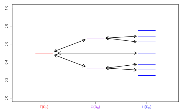
   Figure 13: Illustration of the counterexample for the transitivity of $\leq_{\text{D-supp}}^{\land\text{-disc}}$ and $\leq_{\text{disp}}^{\land\text{-disc}}$ as given in the proof of Theorem 4.2b). The pairs of constant intervals, of which the lengths are to be compared with respect to $\leftrightharpoons_{\land}$, are identified by double-sided arrows. Each constant interval is represented by the value that the corresponding cdf takes on there.

   An illustration of which pairs of constant intervals are compared among the three cdf’s is given in Figure 13. Because of

   $$x_{2}-x_{1}=1\leq 2=c_{y}=y_{2}-y_{1}=y_{3}-y_{2},$$

   $F\leq_{\text{D-supp}}^{\land\text{-disc}}G$ holds, and since

   $$y_{2}-y_{1}=c_{y}=2 \leq 3=c_{z}=z_{3}-z_{2}=z_{4}-z_{3}\quad\text{and}$$

   $$y_{3}-y_{2}=c_{y}=2 \leq 3=c_{z}=z_{6}-z_{5}=z_{7}-z_{6},$$

   $G\leq_{\text{D-supp}}^{\land\text{-disc}}H$ holds. However,

   $$x_{2}-x_{1}=1>\tfrac{1}{2}=\delta=z_{5}-z_{4}$$

   contradicts $F\leq_{\text{D-supp}}^{\land\text{-disc}}H$ and thereby contradicts the transitivity of $\leq_{\text{D-supp}}^{\land\text{-disc}}$ and of $\leq_{\text{disp}}^{\land\text{-disc}}$.

Due to Proposition 3.3, any discrete dispersion order $\leq_{\text{D}}$ that is equivalent to $\leq_{\text{disp}}$ if $F(D_{F})\subseteq G(D_{G})$ compares the lengths of constant intervals in a pointwise fashion that is dictated by the candidate for the less dispersed cdf $F$. This, however, makes it possible to construct a counterexample for the transitivity of $\leq_{\text{D}}$ similar to the one in the proof of Theorem 4.2b). The general approach is to choose $F,G\in\mathcal{D}_{0}$ with $F(D_{F})\cap G(D_{G})=\emptyset$ and both sets being small. Then, $H\in\mathcal{D}_{0}$ is chosen in such a way that $H(D_{H})$ is a disjoint union of one set of points close to the elements of $F(D_{F})$ and another set of points close to the elements of $G(D_{G})$. As a result, the constant intervals of $H$ to be compared with those of $F$ are not compared with any constant intervals of $G$ because of this disjoint split. The transitivity of $\leq_{\text{D}}$ can be contradicted by choosing the lengths of the involved intervals accordingly. Graphically, the situation should be similar to what is depicted in Figure 13.

Proof of Theorem 4.3.

1. According to Example 3.6b), condition (2) is equivalent to $c_{F}\leq c_{G}$. However, because of $x_{a}-x_{a-1}=c_{F}$ and $y_{b}-y_{b-1}=c_{G}$ for all $a\in\underline{A},b\in\underline{B}$, $c_{F}\leq c_{G}$ is also equivalent to both $F\leq_{\text{disp}}^{\lor\text{-disc}}G$ and $F\leq_{\text{disp}}^{\land\text{-disc}}G$.

2. Let $F$, $G$ and $H$ be cdf’s of lattice distributions with distances $c_{F},c_{G},c_{H}>0$ between neighbouring support points. Since $\leq_{\text{D-pm}}^{\text{disc}}$ is transitive as shown in the proof of Theorem 4.2b) and $c_{F}\leq c_{G}$ combined with $c_{G}\leq c_{H}$ implies $c_{F}\leq c_{H}$, the order $\leq_{\text{disp}}^{\text{disc}}$ is transitive on the set of all lattice distributions, and the assertion follows from part a).

Proof of Theorem 4.4.

We start by proving that (i) and (iii) are equivalent.

1. Let $r\in(0,1)\setminus\left(F(D_{F})\cup G(D_{G})\right)$, which is possible since $F(D_{F})\cup G(D_{G})$ is at most countable and $(0,1)$ is uncountable. Now let $a_{r}=\min\{a\in A:F(x_{a})\geq r\}$ (which exists since $r<1=\sup F(\operatorname{supp}(F))$ holds and thus, there exists an $a\in A$ such that $r\in(F(x_{a-1}),F(x_{a}))$) and $b_{r}=\min\{b\in B:G(y_{b})\geq r\}$. Then, $a_{r}\leftrightharpoons b_{r}$ and, by assumption, $F(x_{a_{r}})-F(x_{a_{r}-1})=p_{a_{r}}=q_{b_{r}}=G(y_{b_{r}})-G(y_{b_{r}-1})$ follows. Rearranging yields

   $$F(x_{a_{r}})-G(y_{b_{r}})=F(x_{a_{r}-1})-G(y_{b_{r}-1}).$$

   Assume $F(x_{a_{r}})>G(y_{b_{r}})$. It follows that $a_{r}\leftrightharpoons b_{r}+1$, yielding $F(x_{a_{r}})-F(x_{a_{r}-1})=p_{a_{r}}=q_{b_{r}+1}=G(y_{b_{r}+1})-G(y_{b_{r}})$. Note that $b_{r}+1\in B$ since $G(y_{b_{r}})<F(x_{a_{r}})\leq 1=\sup G(\operatorname{supp}(G))$. Because of $G(y_{b_{r}})>F(x_{a_{r}-1})$, it follows that $G(y_{b_{r}+1})>F(x_{a_{r}})$, thus yielding $a_{r}+1\leftrightharpoons b_{r}+1$. Now the same line of reasoning applied to $a_{r}$ and $b_{r}$ can also be applied to $a_{r}+1$ and $b_{r}+1$. Inductively, it follows that $p_{a_{r}}=p_{\alpha}=q_{\beta}$ for all $\alpha\in A\cap[a_{r},\infty)$ and all $\beta\in B\cap[b_{r},\infty)$. We now know that there exist $c_{A},c_{B}\in\mathbb{N}_{0}$ such that

   $$F(x_{a_{r}})+c_{A}\cdot p_{a_{r}}=F(x_{a_{r}})+\sum_{a_{r}+1}^{\sup A}p_{\alpha}=1=G(y_{b_{r}})+\sum_{\beta=b_{r}+1}^{\sup B}p_{\beta}=G(y_{b_{r}})+c_{B}\cdot p_{a_{r}},$$

   which, since $0<F(x_{a_{r}})-G(y_{b_{r}})<p_{a_{r}}$ (otherwise $a_{r}\leftrightharpoons b_{r}$ would not hold), yields

   $$0=F(x_{a_{r}})-G(y_{b_{r}})+p_{a_{r}}(c_{A}-c_{B})\neq 0,$$

   a contradiction. By symmetry, the case $G(y_{b_{r}})>F(x_{a_{r}})$ also yields a contradiction, leaving only $F(x_{a_{r}})=G(y_{b_{r}})$. It immediately follows that $a_{r}\leftrightharpoons b_{r}$ and $a_{r}+1\leftrightharpoons b_{r}+1$, yielding $p_{a_{r}}=q_{b_{r}}$ and $p_{a_{r}+1}=q_{b_{r}+1}$. This also yields $F(x_{a_{r}-1})=G(y_{b_{r}-1})$ and $F(x_{a_{r}+1})=G(y_{b_{r}+1})$. Inductively, we obtain $p_{a_{r}+d}=q_{b_{r}+d}$ and $F(x_{a_{r}+d})=G(y_{b_{r}+d})$ for all $d\in\mathbb{Z}$ such that $a_{r}+d\in A$ and $b_{r}+d\in B$. Furthermore, $a_{r}+d=\min A$ is equivalent to $b_{r}+d=\min B$ for all $d\in\mathbb{Z}$ and the same is true for the maximums of $A$ and $B$. It follows that $F(\operatorname{supp}(F))=G(\operatorname{supp}(G))$ and, since the indexing sets are uniquely determined by the supports, $A=B$ follows along with $a_{r}=b_{r}$. The sets of pairs of indices to be compared are given by $R(\leftrightharpoons)=\{(a,a):a\in A\}$ and $R(\leftrightharpoons_{\land})=\{(a,a):a\in\underline{A}\}$.

   Now define $\lambda=y_{a_{r}}-x_{a_{r}}$. Let $\alpha\in A$ and, without restriction, let $\alpha\geq a_{r}$. Then,

   $$y_{\alpha}-x_{\alpha}=y_{a_{r}}-x_{a_{r}}+\sum_{j=a_{r}+1}^{\alpha}\left((y_{j}-y_{j-1})-(x_{j}-x_{j-1})\right)=y_{a_{r}}-x_{a_{r}}=\lambda$$

   follows from $F=_{\text{disp}}^{\land\text{-disc}}G$. Overall, we obtain $(B,(y_{j},q_{j})_{j\in B})=(A,(x_{j}+\lambda,p_{j})_{j\in A})$ and since the indexing set and the identifying sequence uniquely identify the corresponding cdf, the assertion follows.

2. The assumption directly implies $B=A$, $y_{j}=x_{j}+\lambda$ and $q_{j}=p_{j}$ for all $j\in A$. The latter observation then implies $F(\operatorname{supp}(F))=G(\operatorname{supp}(G))$ as well as $R(\leftrightharpoons)=\{(a,a):a\in A\}$ and $R(\leftrightharpoons_{\land})=\{(a,a):a\in\underline{A}\}$. While $F=_{\text{D-pm}}^{\text{disc}}G$ is now trivial, $F=_{\text{D-supp}}^{\land\text{-disc}}G$ follows from $(x_{a}+\lambda)-(x_{a-1}+\lambda)=x_{a}-x_{a-1}$ for all $a\in\underline{A}$, thus concluding the proof.

Since $\leq_{\text{disp}}^{\land\text{-disc}}$ is a weakening of $\leq_{\text{disp}}^{\lor\text{-disc}}$, the implication ‘(ii)$\Rightarrow$(i)’ is true generally. For the remaining implication, it is sufficient to show $F\leq_{\text{disp}}^{\land\text{-disc}}G\Leftrightarrow F\leq_{\text{disp}}^{\lor\text{-disc}}G$ for all $F,G\in\mathcal{D}_{0}$ with $F(\operatorname{supp}(F))=G(\operatorname{supp}(G))$. Assuming $F(\operatorname{supp}(F))=G(\operatorname{supp}(G))$ directly implies $R(\leftrightharpoons)=\{(a,a):a\in A\}$, where $A$ is the indexing set of either cdf. This yields

$$R(\leftrightharpoons_{\land})=\{(a,a):a\in\underline{A}\}=R(\leftrightharpoons_{\lor}),$$

thus ensuring the equivalence of $\leq_{\text{disp}}^{\land\text{-disc}}$ and $\leq_{\text{disp}}^{\lor\text{-disc}}$ and concluding the proof.

Proof of Proposition 4.5.

If $F(D_{F})\subseteq G(D_{G})$, the order $\leq_{\text{disp}}^{\land\text{-disc}}$ is equivalent to $\leq_{\text{disp}}$ and the assertion follows. Otherwise, let $a\in\underline{A}$ such that $F(x_{a-1})\in F(D_{F})\setminus G(D_{G})\neq\emptyset$. It follows that

$$\operatorname{NN}_{F}^{G}(a)\ni\sup(G(D_{G})\cap(0,F(x_{a-1})])<F(x_{a-1})<\inf(G(D_{G})\cap[F(x_{a-1}),1))\in\operatorname{NN}_{F}^{G}(a).$$

Hence, $|\operatorname{NN}_{F}^{G}(a)|=2$, and we choose $b\in\overline{\underline{B}}$ such that $\operatorname{NN}_{F}^{G}(a)=\{G(y_{b}),G(y_{b-1})\}$. (Note that $\overline{\underline{B}}\neq\emptyset$ since $|B|\geq 3$ follows from Lemma 3.16.) Particularly, this means that $a\leftrightharpoons_{\land}b+1$ and, therefore, $x_{a}-x_{a-1}\leq y_{b+1}-y_{b}$. Due to Lemma 3.16 and the beginning of the proof of Proposition 3.17, for all $j\in\underline{A},j\geq a$, there exists a $k_{j}\in\underline{B},k_{j}\geq k_{a}=b+1$ such that $G(y_{k_{j}-1})=\inf(G(D_{G})\cap[F(x_{j-1}),1))\in\operatorname{NN}_{F}^{G}(j)$. It follows that $j\leftrightharpoons_{\land}k_{j}$ and, particularly, $j-1\leftrightharpoons k_{j}-1$ for all $j\in\underline{A},j\geq a$. Moreover, the $k_{j}$’s are pairwise distinct. To see this, let $i,j\in\underline{A}\cap[a,\infty)$ with $i>j$; then we have

$$F(x_{j-1})\leq F(x_{i-2})=F(x_{i-1})-p_{i-1}\leq G(y_{k_{i}-1})-q_{k_{i}-1}=G(y_{k_{i}-2}),$$

which implies $G(y_{k_{j}-1})\leq G(_{k_{i}-1})$ and $k_{j}\leq k_{i}-1<k_{i}$. It follows that

$$\sum_{j=a}^{\sup\underline{A}}(x_{j}-x_{j-1})\leq\sum_{j=a}^{\sup\underline{A}}(y_{k_{j}}-y_{k_{j}-1})\leq\sum_{k=b+1}^{\sup\underline{B}}(y_{k}-y_{k-1}).$$ (12)

Instead of using the index $a$ as a starting point upwards, we can also use it as a starting point downwards. It follows from the structure of the set $\operatorname{NN}_{F}^{G}(a)$ that $a\leftrightharpoons_{\land}b$ holds and, subsequently, $x_{a}-x_{a-1}\leq y_{b}-y_{b-1}$. By Lemma 3.16, we obtain that, for all $j\in\underline{A},j\leq a$, there exists a $\ell_{j}\in\underline{B},\ell_{j}\leq\ell_{a}=b$ such that $G(y_{\ell_{j}-1})=\sup(G(D_{G})\cap(0,F(x_{j-1})])\in\operatorname{NN}_{F}^{G}(j)$. As before, it follows that $j\leftrightharpoons_{\land}\ell_{j}$ and, particularly, $j\leftrightharpoons\ell_{j}$ for all $j\in\underline{A},j\leq a$. To see that the $\ell_{j}$’s are also pairwise distinct, let $i,j\in\underline{A}\cap(-\infty,a]$ with $i>j$, yielding

$$F(x_{i-1})\geq F(x_{j})=F(x_{j-1})+p_{j}\geq G(y_{\ell_{j}-1})+q_{\ell_{j}}=G(y_{\ell_{j}})$$

and, therefore, $\ell_{i}\geq\ell_{j}+1>\ell_{j}$. It follows that

$$\sum_{j=\inf\underline{A}}^{a}(x_{j}-x_{j-1})\leq\sum_{j=\inf\underline{A}}^{a}(y_{\ell_{j}}-y_{\ell_{j}-1})\leq\sum_{\ell=\inf\underline{B}}^{b}(y_{\ell}-y_{\ell-1}).$$ (13)

By combining (12) and (13), we obtain

$$\lambda^{1}(D_{F})=\sum_{j=\inf\underline{A}}^{\sup\underline{A}}(x_{j}-x_{j-1})<\sum_{j=\inf\underline{A}}^{\sup\underline{A}}(x_{j}-x_{j-1})+(x_{a}-x_{a-1})\leq\sum_{k=\inf\underline{B}}^{\sup\underline{B}}(y_{k}-y_{k-1})=\lambda^{1}(D_{G}),$$

if $\lambda^{1}(D_{F})<\infty$. Otherwise, we obtain that $D_{G}$ also has infinite Lebesgue measure, since then the leftmost sum in (12) or (13) is already infinite.

Proof of Proposition 4.6.

Similarly as in the proof of Proposition 4.5, Lemma 3.16 states that for all $a\in\underline{A}$, there exists a $b_{a}\in\underline{B}$ such that $G(y_{b_{a}-1})=\sup(G(D_{G})\cap(0,F(x_{a-1})])\in\operatorname{NN}_{F}^{G}(a)$, implying $a\leftrightharpoons_{\land}b_{a}$. As shown for Proposition 4.5, these $b_{a}$’s are pairwise distinct. It follows for all $a\in A$ that

$$x_{a}=\min(\operatorname{supp}(F))+\sum_{j=\min\underline{A}}^{a}(x_{j}-x_{j-1}) \leq\min(\operatorname{supp}(G))+\sum_{j=\min\underline{A}}^{a}(y_{b_{j}}-y_{b_{j}-1})$$

$$\leq\min(\operatorname{supp}(G))+\sum_{k=\min\underline{B}}^{b_{a}}(y_{k}-y_{k-1})=y_{b_{a}}.$$

Note that for all $(a,b)\in R(\leftrightharpoons)$, $b\geq b_{a}$ holds because of $G(y_{b})>F(x_{a-1})\geq G(y_{b_{a}-1})$ and the maximality of $b_{a}$. This means that, for all $(a,b)\in R(\leftrightharpoons)$, we obtain $x_{a}\leq y_{b_{a}}\leq y_{b}$. According to Definition 3.7, this is equivalent to $F\leq_{\text{st}}G$.

Proof of Theorem 4.7.

Let $(a,b),(\alpha,\beta)\in R(\leftrightharpoons)$. For better cross-reference, we divide the proof into three parts.

1. In this part, we show by contradiction that $|x_{\alpha}-x_{a}|>|y_{\beta}-y_{b}|$ implies $|\alpha-a|=|\beta-b|+1$. To this end, we first assume $|\alpha-a|\leq|\beta-b|$. Without restriction, let $\alpha\geq a$. If $\alpha=a$, then $|x_{\alpha}-x_{a}|=0\leq|y_{\beta}-y_{b}|$ follows, contradicting the assumption. Hence, it remains to consider the case $\alpha>a$. Because of $a\leftrightharpoons b$ and $\alpha\leftrightharpoons\beta$, we obtain

   $$G(y_{b-1})<F(x_{a})\leq F(x_{\alpha-1})<G(y_{\beta}),$$ (14)

   yielding $\beta\geq b$. We either have $G(y_{\beta-1})\leq F(x_{\alpha-1})$, yielding $G(y_{\beta-1})=\sup(G(D_{G})\cap(0,F(x_{\alpha-1})])\in\operatorname{NN}_{F}^{G}(\alpha)$; in this case we define $k_{\alpha}=\beta$. Or we have $G(y_{\beta-1})>F(x_{\alpha-1})$, implying that there exists a $k_{\alpha}\leq\beta$ such that $G(y_{k_{\alpha}-1})=\inf(G(D_{G})\cap[F(x_{\alpha-1}),1))\in\operatorname{NN}_{F}^{G}(\alpha)$. Note that $k_{\alpha}>b$ holds because of $G(y_{k_{\alpha}-1})\geq F(x_{\alpha-1})$ and (14). So, considering both cases as well as Proposition 3.17a), there exists a $k_{\alpha}\in\{b+1,\ldots,\beta\}$ such that $\alpha\leftrightharpoons_{\land}k_{\alpha}$.

   It follows that $\alpha-1\leftrightharpoons k_{\alpha}-1$ and we can repeat the line of argument from above with $\alpha-1$ taking the role of $\alpha$ and $k_{\alpha}-1$ taking the role of $\beta$, as long as $\alpha-1>a$. We then obtain a $k_{\alpha-1}\in\{b+1,\ldots,k_{\alpha}-1\}$ such that $\alpha-1\leftrightharpoons_{\land}k_{\alpha-1}$ and can repeat the line of argument again, starting with $\alpha-2\leftrightharpoons k_{\alpha-1}-1$ as long as $\alpha-2>a$. Iteratively, we obtain the following statement:

   $$\forall j\in\{a+1,\ldots,\alpha\}\;\exists\text{ pairwise distinct }k_{j}\in\{b+1,\ldots,\beta\}\text{ such that }j\leftrightharpoons_{\land}k_{j}.$$

   Since $F\leq_{\text{D-supp}}^{\land\text{-disc}}G$ holds, it follows

   $$|x_{\alpha}-x_{a}|=x_{\alpha}-x_{a} =\sum_{j=a+1}^{\alpha}(x_{j}-x_{j-1})$$

   $$\leq\sum_{j=a+1}^{\alpha}(y_{k_{j}}-y_{k_{j}-1})$$

   $$\leq\sum_{k=b+1}^{\beta}(y_{k}-y_{k-1})=y_{\beta}-y_{b}=|y_{\beta}-y_{b}|,$$

   a contradiction to the assumption $|x_{\alpha}-x_{a}|>|y_{\beta}-y_{b}|$. This closes the case $|\alpha-a|\leq|\beta-b|$.

   Second, we assume $|\alpha-a|\geq|\beta-b|+2$. Again, let $\alpha\geq a$. Because of $\alpha-a=|\alpha-a|\geq|\beta-b|+2\geq 2$, we have $\alpha>a$. By combining $a\leftrightharpoons b$ and $\alpha\leftrightharpoons\beta$, we obtain (14) and $\beta\geq b$, as before. It follows from (14) that, for every $j\in\{a+1,\ldots,\alpha-1\}$, there exists a $k\in\{b,\ldots,\beta\}$ such that $j\leftrightharpoons k$. More specifically, we define $k_{j}=\min\{k\in\{b,\ldots\beta\}:j\leftrightharpoons k\}$ for every $j\in\{a+1,\ldots,\alpha-1\}$. These $k_{j}$ are pairwise distinct; otherwise there would exist indices $i,j\in\{a+1,\ldots,\alpha-1\},i\neq j$ (without restriction $i<j$) such that $k_{i}=k_{j}$. This implies $G(y_{k_{i}-1})\leq F(x_{i-1})$ because of the minimality of $k_{i}$. We obtain

   $$G(y_{k_{i}})=G(y_{k_{i}-1})+q_{k_{i}}\leq F(x_{i-1})+p_{i}=F(x_{i})\leq F(x_{j-1})<G(y_{k_{j}}),$$

   yielding a contradiction, and thereby proving that the mapping $j\mapsto k_{j}$ is injective. The cardinal number of the domain $\{a+1,\ldots,\alpha-1\}$ of that mapping is $|\alpha-a|-1$ and by assumption larger than or equal to the cardinal number $|\beta-b|+1$ of its codomain $\{b,\ldots,\beta\}$. For $|\alpha-a|>|\beta-b|+2$, this directly contradicts the injectivity of the mapping. For $|\alpha-a|=|\beta-b|+2$, it follows that the mapping is bijective and we obtain

   $$F(x_{\alpha-1})-F(x_{a})=\sum_{j=a+1}^{\alpha-1}p_{j}\geq\sum_{j=a+1}^{\alpha-1}q_{k_{j}}=\sum_{k=b}^{\beta}q_{k}=G(y_{\beta})-G(y_{b-1}).$$

   This, however, contradicts (14). Thus, we have shown the implication

   $$|x_{\alpha}-x_{a}|>|y_{\beta}-y_{b}|\Longrightarrow|\alpha-a|=|\beta-b|+1\quad\forall(a,b),(\alpha,\beta)\in R(\leftrightharpoons)$$ (15)

   by excluding all other possibilities.

2. It becomes apparent in Part 3 of the proof that pairs $(a,b),(\alpha,\beta)\in R(\leftrightharpoons)$ satisfying $|x_{\alpha}-x_{a}|\leq|y_{\beta}-y_{b}|$ are easy to deal with. Therefore, the critical situation $|x_{\alpha}-x_{a}|>|y_{\beta}-y_{b}|$ is of particular interest. Considering in the final result (15) of Part 1, this implies $|\alpha-a|=|\beta-b|+1$. It is the purpose of Part 2 to analyze the situation for these kinds of pairs more closely, so let $(a,b),(\alpha,\beta)\in R(\leftrightharpoons)$ with $|\alpha-a|=|\beta-b|+1$. Furthermore, let $\alpha>a$. As in Part 1, we obtain (14) and thereby $\beta\geq b$. It follows from (14) and $a\leftrightharpoons b$ that, for every $j\in\{a,\ldots,\alpha-1\}$, there exists a $k\in\{b,\ldots,\beta\}$ such that $j\leftrightharpoons k$. We consider the mapping

   $$\varphi_{1}:\{a,\ldots,\alpha-1\}\to\{b,\ldots,\beta\},\quad j\mapsto k_{j}=\max\{k\in\{b,\ldots\beta\}:j\leftrightharpoons k\}.$$

   To see that $\varphi_{1}$ is strictly increasing, let $j,j+1\in\{a,\ldots,\alpha-1\}$. It follows from the maximality of $k_{j+1}$ that $G(y_{k_{j+1}})\geq F(x_{j+1})$, yielding

   $$G(y_{k_{j+1}-1})=G(y_{k_{j+1}})-q_{k_{j+1}}\geq F(x_{j+1})-p_{j+1}=F(x_{j})>G(y_{k_{j}-1})$$

   and, thereby, $k_{j+1}>k_{j}$. Thus, $\varphi_{1}$ is strictly increasing and therefore also injective. Since $\alpha-a-1=\beta-b$ means that the domain and the codomain of $\varphi_{1}$ have the same cardinal number, the mapping is bijective. This means that

   $$a\leftrightharpoons b,\ a+1 \hskip 2.84526pt\leftrightharpoons \;b+1,\ \ldots,\ \alpha-2 \hskip 2.84526pt\leftrightharpoons \;\beta-1,\ \alpha-1 \hskip 2.84526pt\leftrightharpoons \;\beta,$$ (16)

   $$a+1 \leftrightharpoons_{\land} \;b+1,\ \ldots,\ \alpha-2 \leftrightharpoons_{\land} \;\beta-1,\ \alpha-1 \leftrightharpoons_{\land} \;\beta.$$ (17)

   Combined with (14), this has the following two implications:

   $$G(y_{b-1})-F(x_{a-1}) =\left(G(y_{\beta})-\sum_{k=b}^{\beta}q_{k}\right)-\left(F(x_{\alpha-1})-\sum_{j=a}^{\alpha-1}p_{j}\right)$$

   $$=G(y_{\beta})-F(x_{\alpha-1})+\sum_{j=a}^{\alpha-1}(p_{j}-q_{k_{j}})\geq G(y_{\beta})-F(x_{\alpha-1})>0,$$ (18)

   $$x_{\alpha-1}-x_{a} =\sum_{j=a+1}^{\alpha-1}(x_{j}-x_{j-1})\leq\sum_{j=a+1}^{\alpha-1}(y_{k_{j}}-y_{k_{j}-1})=\sum_{k=b+1}^{\beta}(y_{k}-y_{k-1})=y_{\beta}-y_{b}.$$ (19)

   It follows from (14), $a\leftrightharpoons b$ and $\alpha\leftrightharpoons\beta$ that, for every $j\in\{a,\ldots,\alpha\}$, there exists a $k\in\{b-1,\ldots,\beta\}$ such that $j\leftrightharpoons k$. Note that $b-1\in B$ because of (18), which implies $G(y_{b-1})>F(x_{a-1})\geq 0$. We now consider the mapping

   $$\varphi_{2}:\{a,\ldots,\alpha\}\to\{b-1,\ldots,\beta\},\quad j\mapsto k_{j}=\min\{k\in\{b-1,\ldots\beta\}:j\leftrightharpoons k\}.$$

   To see that $\varphi_{2}$ is strictly increasing, let $j,j+1\in\{a,\ldots,\alpha\}$. It follows from the minimality of $k_{j}$ that $G(y_{k_{j}-1})\leq F(x_{j-1})$, yielding

   $$G(y_{k_{j}})=G(y_{k_{j}-1})+q_{k_{j}}\leq F(x_{j-1})+p_{j}=F(x_{j})=F(x_{(j+1)-1})<G(y_{k_{j+1}})$$

   and, thereby, $k_{j}<k_{j+1}$. Thus, $\varphi_{2}$ is strictly increasing and therefore also injective. Since $\alpha-a=\beta-b+1$ means that the domain and the codomain of $\varphi_{2}$ have the same cardinal number, the mapping is bijective. This means that

   $$a\leftrightharpoons b-1,\ a+1 \hskip 2.84526pt\leftrightharpoons \;b,\ \ldots,\ \alpha-1 \hskip 2.84526pt\leftrightharpoons \beta-1,\ \alpha \hskip 2.84526pt\leftrightharpoons \;\beta,$$ (20)

   $$a+1 \leftrightharpoons_{\land} \;b,\ \ldots,\ \alpha-1 \leftrightharpoons_{\land} \;\beta-1,\ \alpha \leftrightharpoons_{\land} \;\beta.$$ (21)

   Combined with (14), this has the following two implications:

   $$F(x_{\alpha-1})-G(y_{\beta-1}) =\left(F(x_{a})+\sum_{j=a+1}^{\alpha-1}p_{j}\right)-\left(G(y_{b-1})+\sum_{k=b}^{\beta-1}q_{k}\right)$$

   $$=F(x_{a})-G(y_{b-1})+\sum_{j=a+1}^{\alpha-1}(p_{j}-q_{k_{j}})\geq F(x_{a})-G(y_{b-1})>0,$$ (22)

   $$x_{\alpha}-x_{a} =\sum_{j=a+1}^{\alpha}(x_{j}-x_{j-1})\leq\sum_{j=a+1}^{\alpha}(y_{k_{j}}-y_{k_{j}-1})=\sum_{k=b}^{\beta}(y_{k}-y_{k-1})=y_{\beta}-y_{b-1}.$$ (23)

3. Recall the definition of $r_{(a,b)}$ in (5) to see that the following holds true for all $t\in\mathbb{R}$:

   $$H_{|X-X^{\prime}|}(t) =\mathbb{P}(|X-X^{\prime}|\leq t)$$

   $$=\sum_{x,x^{\prime}\in\operatorname{supp}(F)}\mathbb{P}(X=x)\mathbb{P}(X^{\prime}=x^{\prime})\mathbbm{1}\{|x-x^{\prime}|\leq t\}$$

   $$=\sum_{a,\alpha\in A}p_{a}p_{\alpha}\mathbbm{1}\{|x_{a}-x_{\alpha}|\leq t\}$$

   $$=\sum_{a,\alpha\in A}\left(\sum_{b\in B:a\leftrightharpoons b}r_{(a,b)}\right)\left(\sum_{\beta\in B:\alpha\leftrightharpoons\beta}r_{(\alpha,\beta)}\right)\mathbbm{1}\{|x_{a}-x_{\alpha}|\leq t\}$$

   $$=\sum_{(a,b),(\alpha,\beta)\in R(\leftrightharpoons)}r_{(a,b)}r_{(\alpha,\beta)}\mathbbm{1}\{|x_{a}-x_{\alpha}|\leq t\}.$$ (24)

   Analogously, we obtain

   $$H_{|Y-Y^{\prime}|}(t)=\mathbb{P}(|Y-Y^{\prime}|\leq t) =\sum_{(a,b),(\alpha,\beta)\in R(\leftrightharpoons)}r_{(a,b)}r_{(\alpha,\beta)}\mathbbm{1}\{|y_{b}-y_{\beta}|\leq t\}$$ (25)

   for all $t\in\mathbb{R}$. The claim of the theorem is equivalent to

   $$0 \leq H_{|X-X^{\prime}|}(t)-H_{|Y-Y^{\prime}|}(t)$$

   $$=\sum_{(a,b),(\alpha,\beta)\in R(\leftrightharpoons)}r_{(a,b)}r_{(\alpha,\beta)}\big{(}\mathbbm{1}\{|x_{\alpha}-x_{a}|\leq t\}-\mathbbm{1}\{|y_{\beta}-y_{b}|\leq t\}\big{)}$$ (26)

   for all $t\in\mathbb{R}$. By Part 1, we have for all $(a,b),(\alpha,\beta)\in R(\leftrightharpoons)$ that

   $$|\alpha-a|\neq|\beta-b|+1\Longrightarrow \;|x_{\alpha}-x_{a}|\leq|y_{\beta}-y_{b}|$$

   $$\Longleftrightarrow \;\big{(}|y_{\beta}-y_{b}|\leq t\Longrightarrow|x_{\alpha}-x_{a}|\leq t\big{)}\quad\forall t\in\mathbb{R}$$

   $$\Longleftrightarrow \;\mathbbm{1}\{|x_{\alpha}-x_{a}|\leq t\}-\mathbbm{1}\{|y_{\beta}-y_{b}|\leq t\}\geq 0\quad\forall t\in\mathbb{R}.$$

   The sums in (24) and (25) can each be split into three separate sums, one with $\alpha>a$, one with $\alpha=a$ and one with $\alpha<a$. Since all the summands in (24) and (25) are symmetric in $(a,b)$ and $(\alpha,\beta)$, the sum with $\alpha>a$ is equal to the sum with $\alpha<a$. Because $\alpha=a$ and $|\alpha-a|=|\beta-b|+1$ are not possible simultaneously, we obtain for all $t\in\mathbb{R}$ that

   $$H_{|X-X^{\prime}|}(t)-H_{|Y-Y^{\prime}|}(t)$$

   $$\qquad=2\sum_{\begin{subarray}{c}(a,b),(\alpha,\beta)\in R(\leftrightharpoons):\\ \alpha>a\end{subarray}}r_{(a,b)}r_{(\alpha,\beta)}\big{(}\mathbbm{1}\{|x_{\alpha}-x_{a}|\leq t\}-\mathbbm{1}\{|y_{\beta}-y_{b}|\leq t\}\big{)}$$

   $$\qquad\phantom{=}\;+\sum_{\begin{subarray}{c}(a,b),(\alpha,\beta)\in R(\leftrightharpoons):\\ \alpha=a\end{subarray}}r_{(a,b)}r_{(\alpha,\beta)}\big{(}\mathbbm{1}\{|x_{\alpha}-x_{a}|\leq t\}-\mathbbm{1}\{|y_{\beta}-y_{b}|\leq t\}\big{)}$$

   $$\qquad\geq 2\sum_{\begin{subarray}{c}(a,b),(\alpha,\beta)\in R(\leftrightharpoons):\\ |\alpha-a|=|\beta-b|+1,\\ \alpha>a\end{subarray}}\bigg{[}r_{(a,b)}r_{(\alpha,\beta)}\big{(}\mathbbm{1}\{x_{\alpha}-x_{a}\leq t\}-\mathbbm{1}\{y_{\beta}-y_{b}\leq t\}\big{)}$$

   $$\qquad\phantom{=}\;+r_{(a,b-1)}r_{(\alpha-1,\beta)}\big{(}\mathbbm{1}\{x_{\alpha-1}-x_{a}\leq t\}-\mathbbm{1}\{y_{\beta}-y_{b-1}\leq t\}\big{)}\bigg{]}.$$ (27)

   For the validity of the inequality we use that, under the assumptions $(a,b),(\alpha,\beta)\in R(\leftrightharpoons)$, $|\alpha-a|=|\beta-b|+1$ and $\alpha>a$, it follows that $(a,b-1),(\alpha-1,\beta)\in R(\leftrightharpoons)$ according to (16) and (20). Note that $|(\alpha-1)-a|\neq|\beta-(b-1)|+1$ holds true in all summands of the last sum, so no summand is used twice in that sum. For the differences of the indicator functions, it holds that

   $$\mathbbm{1}\{x_{\alpha}-x_{a}\leq t\}-\mathbbm{1}\{y_{\beta}-y_{b}\leq t\}=-1 \Longleftrightarrow t\in[y_{\beta}-y_{b},x_{\alpha}-x_{a})\quad\text{ and }$$

   $$\mathbbm{1}\{x_{\alpha-1}-x_{a}\leq t\}-\mathbbm{1}\{y_{\beta}-y_{b-1}\leq t\}=1 \Longleftrightarrow t\in[x_{\alpha-1}-x_{a},y_{\beta}-y_{b-1})$$

   for all $(a,b),(\alpha,\beta)\in R(\leftrightharpoons)$ with $|\alpha-a|=|\beta-b|+1$ and $\alpha>a$. Because of (19) and (23), $[y_{\beta}-y_{b},x_{\alpha}-x_{a})\subseteq[x_{\alpha-1}-x_{a},y_{\beta}-y_{b-1})$ follows, yielding

   $$\mathbbm{1}\{x_{\alpha}-x_{a}\leq t\}-\mathbbm{1}\{y_{\beta}-y_{b}\leq t\}=-1\Longrightarrow\mathbbm{1}\{x_{\alpha-1}-x_{a}\leq t\}-\mathbbm{1}\{y_{\beta}-y_{b-1}\leq t\}=1.$$

   This means that in order to prove that (27) is larger than or equal to zero and thereby complete the proof, it remains to show that $r_{(a,b)}r_{(\alpha,\beta)}\leq r_{(a,b-1)}r_{(\alpha-1,\beta)}$ holds for all $(a,b),(\alpha,\beta)\in R(\leftrightharpoons)$ with $|\alpha-a|=|\beta-b|+1$ and $\alpha>a$. In that setting, by combining (18) and (22), we obtain

   $$r_{(a,b)}r_{(\alpha,\beta)} =\big{(}F(x_{a})-G(y_{b-1})\big{)}\big{(}G(y_{\beta})-F(y_{\alpha-1})\big{)}$$

   $$\leq\big{(}F(x_{\alpha-1})-G(y_{\beta-1})\big{)}\big{(}G(y_{b-1})-F(x_{a-1})\big{)}=r_{(\alpha-1,\beta)}r_{(a,b-1)}.$$

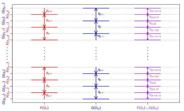
Figure 14: Exemplary visualization of crucial situation in the proof of Theorem 4.7. The horizontal lines represent the elements of the sets given on the x-axis. The double-sided arrows and the variable names next to them represent the distances between those horizontal lines.

The starting point of the proof of Theorem 4.7 is the representation of the cdf of $|X-X^{\prime}|$ given in (24) as a sum of products $r_{(a,b)}r_{(\alpha,\beta)}$ of probability masses on two given pairs in $R(\leftrightharpoons)$. An analogous sum can be used to represent the cdf of $|Y-Y^{\prime}|$ with the sole difference that each summand is multiplied with a different indicator than for $|X-X^{\prime}|$. The implication (15), which is shown in Part 1 of the proof, states the indicators for a given summand are one for $|X-X^{\prime}|$ and zero for $|Y-Y^{\prime}|$ if and only if $|\alpha-a|=|\beta-b|+1$, which is a crucial restriction. In Part 3 of the proof, it is shown that, for every two pairs of indices $(a,b),(\alpha,\beta)$ for which this occurs, there exists another set of indices $(a,b-1),(\alpha-1,\beta)$ for which the indicators take the opposite values. Additionally, it is shown that $r_{(a,b-1)}r_{(\alpha-1,\beta)}$, the coefficient for the latter set, is always larger than $r_{(a,b)}r_{(\alpha,\beta)}$, the coefficient for the former set. So for every negative summand in the difference of the two cdf’s, there exists a corresponding positive summand with equal or larger absolute value. The situation is illustrated in Figure 14. The fact that the values of $F(D_{F})$ and $G(D_{G})$ in question are alternating, follows from $|\alpha-a|=|\beta-b|+1$ and is derived in Part 2 of the proof. The plot also hints at the fact that, for reasons of symmetry, $(a+1,b),(\alpha,\beta+1)$ would have been a viable alternative of $(a,b-1),(\alpha-1,\beta)$ in its role as compensatory set of indices.

Proof of Lemma 4.8.

Let $X\sim F$, $Y\sim G$ and, as assumed $\mathbb{E}[X]=\mathbb{E}[Y]$ with $F\neq G$.

1. For all $a\in A$, define the set $B_{a}=\{b\in\underline{B}:F(x_{a-1})\leq G(y_{b-1})\leq F(x_{a})\}$. Note that, for all $a\in\underline{A}$, $B_{a}\neq\emptyset$ holds. Otherwise, there would exist a $b\in\underline{B}$ such that $G(y_{b-1})<F(x_{a-1})<F(x_{a})<G(y_{b})$, yielding $q_{b}>p_{a}$ in spite of $a\leftrightharpoons b$ and thus contradicting $F\leq_{\text{disp}}^{\land\text{-disc}}G$. With similar reasoning, $B_{\min A}\neq\emptyset$ follows (provided that the minimum exists). We now prove part a) by contradiction and therefore assume that $x_{a}\leq y_{b-1}$ or $y_{b}<x_{a}$ holds for all $b\in B_{a}$ and all $a\in A$. This is contradicted by case distinction.

   1. $x_{a}\leq y_{b-1}\ \forall(a,b)\in\bigcup_{a\in A}\left(\{a\}\times B_{a}\right)$
      Let $a\in\underline{A}$. Obviously, $a\leftrightharpoons b$ holds for all $b\in B_{a}$, except if $G(y_{b-1})=F(x_{a})$. More precisely, if there exists a $b\in B$ such that $F(x_{a-1})=G(y_{b-1})$, then $\{b\in B:a\leftrightharpoons b\}\subseteq B_{a}$. Otherwise, we have $\{b\in B:a\leftrightharpoons b\}\subseteq B_{a}\cup\{\min B_{a}-1\}$. Overall, $x_{a}\leq y_{b}$ follows for all $(a,b)\in R(\leftrightharpoons)\cap(\underline{A}\times B)$. (This is because, for all $a\in\underline{A}$, we have $x_{a}\leq y_{b-1}<y_{b}$ for $b\in B_{a}$ and $x_{a}\leq y_{\min B_{a}-1}$ by assumption.)

      Now, let $a=\min A$ and assume that this minimum exists. Similarly as before, we have

      $$\{b\in B:a\leftrightharpoons b\}\subseteq B_{a}\cup\{\min B_{a}-1\}=B_{a}\cup\{\min B\}$$

      and we can infer $x_{a}\leq y_{b}$ for all $(a,b)\in R(\leftrightharpoons)\cap(\{\min A\}\times B)$. Combined with the results for $a\in\underline{A}$, it follows that $x_{a}\leq y_{b}$ holds for all $(a,b)\in R(\leftrightharpoons)$. Furthermore, at least one of these inequalities is strict since equality for all these pairs would imply $F=G$. It follows

      $$0=\mathbb{E}[Y]-\mathbb{E}[X]=\sum_{(a,b)\in R(\leftrightharpoons)}r_{(a,b)}(y_{b}-x_{a})>0,$$

      a contradiction.

   2. $y_{b}<x_{a}\ \forall(a,b)\in\bigcup_{a\in A}\left(\{a\}\times B_{a}\right)$
      Let $a\in A$. Analogously to Case 1, it can be shown that $\{b\in B:a\leftrightharpoons b\}\subseteq B_{a}\cup\{\min B_{a}-1\}$. If $b\in B_{a}$, $y_{b}<x_{a}$ holds by assumption; if $b=\min B_{a}-1$, $y_{b}<y_{\min B_{a}}<x_{a}$ holds. Overall, we have $y_{b}<x_{a}$ for all $(a,b)\in R(\leftrightharpoons)$, yielding

      $$0=\mathbb{E}[X]-\mathbb{E}[Y]=\sum_{(a,b)\in R(\leftrightharpoons)}r_{(a,b)}(x_{a}-y_{b})>0,$$ (28)

      a contradiction.

   The remaining cases all consist of $x_{a}\leq y_{b-1}$ holding for some pairs $(a,b)\in\bigcup_{a\in A}\left(\{a\}\times B_{a}\right)$ and $y_{b}<x_{a}$ holding for others. For that, we order all these pairs from low to high, or, in other words, primarily by $a\in A$ and secondarily by $b\in B_{a}$, i.e.

   $$\ldots,(a-1,\min B_{a-1}),\ldots,(a-1,\max B_{a-1}),(a,\min B_{a}),\ldots,(a,\max B_{a}),\ldots.$$

   This gives us three possible kinds of successive pairs. The first one is $(a,b),(a,b+1)$, where $a\in A$ and $b,b+1\in B_{a}$ (denoted by (P1)). Both the second and the third kind are of the form $(a,\max B_{a}),(a+1,\min B_{a+1})$ for an $a\in\overline{A}$. If $G(y_{\max B_{a}-1})\in F(D_{F})$, then $\max B_{a}=\min B_{a+1}$ holds by definition of $B_{a}$. This gives the second kind of successive pairs, which is of the form $(a,b),(a+1,b)$, where $a\in\overline{A}$ and $G(y_{b-1})=F(x_{a})$ (denoted by (P2)). (Note that $G(y_{\max B_{a}-1})=F(x_{a-1})$ is not possible because $G(y_{\max B_{a}})>F(x_{a})$ then contradicts $q_{\max B_{a}}\leq p_{a}$ and therefore $a\leftrightharpoons\max B_{a}$, and $G(y_{\max B_{a}})\leq F(x_{a})$ then contradicts the maximality of $\max B_{a}$.) If $G(y_{\max B_{a}-1})\notin F(D_{F})$, then $\max B_{a}=\min B_{a+1}-1$ holds. This gives us the third kind of successive pairs, which is of the form $(a,b),(a+1,b+1)$, where $a\in\overline{A}$ and $b=\max B_{a}$ (denoted by (P3)).

   For each of these kinds of successive pairs, $x_{a}\leq y_{b-1}$ can hold for the former and $y_{b}<x_{a}$ can hold for the latter or vice versa. Overall, this gives us six cases that remain to be considered.

   1. (P1) with $x_{a}\leq y_{b-1}$ and $y_{b+1}<x_{a}$
      This directly gives $y_{b+1}<x_{a}\leq y_{b-1}$, a contradiction.

   2. (P1) with $y_{b}<x_{a}$ and $x_{a}\leq y_{b}$
      These two statements directly contradict each other.

   3. (P2) with $x_{a}\leq y_{b-1}$ and $y_{b}<x_{a+1}$
      Since $G(y_{b-1})=F(x_{a})$ holds for any successive pair of index pairs of the second kind, it follows $a+1\leftrightharpoons_{\land}b$. Then,

      $$x_{a+1}=x_{a}+(x_{a+1}-x_{a})\leq y_{b-1}+(x_{a+1}-x_{a})\leq y_{b-1}+(y_{b}-y_{b-1})=y_{b},$$ (29)

      which contradicts the assumption $y_{b}<x_{a+1}$.

   4. (P2) with $y_{b}<x_{a}$ and $x_{a+1}\leq y_{b-1}$
      This directly gives $x_{a+1}\leq y_{b-1}<y_{b}<x_{a}$, a contradiction.

   5. (P3) with $x_{a}\leq y_{b-1}$ and $y_{b+1}<x_{a+1}$
      Since $G(y_{b-1})<F(x_{a})<G(y_{b})$ holds for any successive pair of pairs of the third kind, it follows from Proposition 3.17a) that $a+1\leftrightharpoons_{\land}b$. Then, (29) again holds, contradicting the assumption $y_{b}<y_{b+1}<x_{a+1}$.

   6. (P3) with $y_{b}<x_{a}$ and $x_{a+1}\leq y_{b}$
      This directly gives $x_{a+1}\leq y_{b}<x_{a}$, a contradiction.

   Now, we have considered all relevant cases and have thereby proved part a).

2. We prove this part by showing that (i) follows, if (ii) does not hold. This is done in several steps.

   1. If (ii) does not hold, part a) yields that there exists a pair $(a,b)\in A\times\overline{B}$ such that $F(x_{a})=G(x_{b})$ and $y_{b}<x_{a}$ or there exists a pair $(a,b)\in\overline{A}\times\overline{B}$ such that $F(x_{a})=G(x_{b})$ and $x_{a+1}\leq y_{b+1}$.

   2. In the first case from Step 1, it directly follows from $b\in\overline{B}$ and $F(x_{a})=G(y_{b})$ that $a\in\overline{A}$. Then, either $x_{a+1}\leq y_{b+1}$ holds (in which case we are finished) or $y_{b+1}<x_{a+1}$. Hence, assume $y_{b+1}<x_{a+1}$. We proceed by showing $b+1\in\overline{B}$. We prove this by contradiction and therefore assume $G(y_{b+1})=1$, from which $1=F(x_{a+1})\geq G(y_{b+1})$ directly follows because of $a+1\leftrightharpoons b+1$. Thus, $p_{a+1}=q_{b+1}$ holds, which yields $R(\leftrightharpoons)\cap(\{a+1\}\times B)=\{(a+1,b+1)\}$. We now seek to show $y_{\beta}<x_{\alpha}$ for all $(\alpha,\beta)\in R(\leftrightharpoons)$, which then implies $\mathbb{E}[Y]<\mathbb{E}[X]$ in the same way as in (28) and thereby concludes the proof of $b+1\in\overline{B}$ by contradiction. Obviously, $y_{\beta}<x_{a}$ is true for all $\beta\in B$ such that $a\leftrightharpoons\beta$ because of $y_{b}<x_{a}$ and since all such $\beta$’s are no larger than $b$. From Proposition 3.17a), it follows that there exists a $\beta_{0}\leq b-1$ such that $a\leftrightharpoons_{\land}\beta_{0}+1$ with $\beta_{0}$ being the largest element of $B$, for which $a-1\leftrightharpoons\beta_{0}$ holds. (This can be achieved by defining $\beta_{0}=\min\operatorname{NN}_{F}^{G}(a)-1$.) From this,

      $$y_{\tilde{\beta}_{0}}<y_{\beta_{0}} =y_{\beta_{0}+1}-(y_{\beta_{0}+1}-y_{\beta_{0}})\leq y_{\beta_{0}+1}-(x_{a}-x_{a-1})$$

      $$\leq y_{b}-(x_{a}-x_{a-1})<x_{a}-(x_{a}-x_{a-1})=x_{a-1}$$

      follows for all $\tilde{\beta}_{0}\in B$ such that $a-1\leftrightharpoons\tilde{\beta}_{0}$. This can be recursively continued for $a-2,a-3,\ldots$ as long as these indices are in $A$. Overall, this proves that $y_{\beta}<x_{\alpha}$ holds for all $(\alpha,\beta)\in R(\leftrightharpoons)$.

   3. Still assuming $y_{b+1}<x_{a+1}$, it follows from Step 2 that $b+1\in\overline{B}$. Now, if $F(x_{a+1})=1$, along with $y_{\beta}<x_{a+1}$ for all $\beta>b+1$, $\mathbb{E}[Y]<\mathbb{E}[X]$ follows similarly as before, leading to a contradiction. Assuming $F(x_{a+1})=1$ along with the existence of a $\beta>b+1$ such that $y_{\beta-1}<x_{a+1}\leq y_{\beta}$ yields that $(a+1,\beta)$ satisfies condition (ii), which also poses a contradiction. Hence, $F(x_{a+1})<1$ and $a+1\in\overline{A}$.

   4. Since (ii) is assumed to not hold, $y_{\beta+1}<x_{a+1}$ follows for all $\beta\in\overline{B}$ with $F(x_{a})<G(y_{\beta})<F(x_{a+1})$. Hence, there exists a $\beta_{1}\in\overline{B}$ with $F(x_{a+1})\leq G(y_{\beta_{1}})<F(x_{a+2})$ and $y_{\beta_{1}}<x_{a+1}<x_{a+2}$. Now we can use our earlier procedure recursively in the following sense. If $G(y_{\beta_{1}})>F(x_{a+1})$, $y_{\beta_{1}+1}<x_{a+2}$ follows since (ii) does not hold. This gives us the setting from the beginning of Step 4 with $(a,\beta)$ replaced by $(a+1,\beta_{1})$. Here, $a+2\in\overline{A}$ is guaranteed since otherwise, $\mathbb{E}[Y]<\mathbb{E}[X]$ would follow. This can be repeated recursively as long as the strict inequality analogous to $G(y_{\beta_{1}})>F(x_{a+1})$ is satisfied. The recursion has to stop at some point (in the sense that equality holds) since otherwise, $\mathbb{E}[Y]<\mathbb{E}[X]$ would follow.

      If $G(y_{\beta_{1}})=F(x_{a+1})$ holds (or an analogous inequality later in the recursion), we can reuse the proof from Step 2 onwards, replacing the pair $(a,b)$ by $(a+1,\beta_{1})$. With this new recursion, we end up at some point with a pair that satisfies condition (i) since, otherwise, the contradiction $\mathbb{E}[Y]<\mathbb{E}[X]$ would follow again.

   5. It remains to consider the second case in Step 1, so that there exists a pair $(a,b)\in\overline{A}\times\overline{B}$ such that $x_{a+1}\leq y_{b+1}$. Here, we can use the exact same procedure as in Steps 2–4, only going through the cdf’s $F$ and $G$ in the opposite direction. The fact that the inequality $x_{a+1}\leq y_{b+1}$ is not a strict inequality does not change anything, because if equality held every time, we would end up with $F=G$, a contradiction. (In Steps 2–4, the contradiction $\mathbb{E}[Y]<\mathbb{E}[X]$ always follows from $y_{\beta}<x_{\alpha}$ holding for all $(\alpha,\beta)\in R(\leftrightharpoons)$. Hence, if the inequality is not strict, $\mathbb{E}[X]=\mathbb{E}[Y]$ can only occur if $y_{\beta}=x_{\alpha}$ holds for all $(\alpha,\beta)\in R(\leftrightharpoons)$. However, in that case, we already have $F=G$.)

Proof of Theorem 4.9.

Assume without restriction that $\mathbb{E}[X]=\mathbb{E}[Y]$ and $F\neq G$. We proceed by showing $F\leq_{\text{dil}}G$ in cases (i) and (ii) of Lemma 4.8b), adopting the notation from there. According to the assumption $\mathbb{E}[X]=\mathbb{E}[Y]$, the characterization of the dilation order given in Proposition 2.3a) and the identity

$$\mathbb{E}[(X-t)_{+}]=\mathbb{E}[X-t]+\mathbb{E}[(X-t)_{-}]=\mathbb{E}[X]-t+\mathbb{E}[(X-t)_{-}]$$

for all $t\in\mathbb{R}$, $F\leq_{\text{dil}}G$ is equivalent to

$$\mathbb{E}[(X-t)_{+}]\leq\mathbb{E}[(Y-t)_{+}]\quad\forall t\geq t_{0}\quad\text{and}\quad\mathbb{E}[(X-t)_{-}]\leq\mathbb{E}[(Y-t)_{-}]\quad\forall t\leq t_{0}$$ (30)

for any $t_{0}\in\mathbb{R}$.

1. Let $(a,b)$ be the pair, the existence of which is guaranteed by (i) in Lemma 4.8b) and choose $t_{0}=\frac{x_{a}+x_{a+1}}{2}$. The first inequality in (30) is now equivalent to

   $$\sum_{(\alpha,\beta)\in R(\leftrightharpoons)}r_{(\alpha,\beta)}((y_{\beta}-t)_{+}-(x_{\alpha}-t)_{+})\geq 0.$$ (31)

   for all $t\geq t_{0}$. The summand corresponding to any pair $(\alpha,\beta)\in R(\leftrightharpoons)$ with $\alpha\leq a$ is zero because $x_{\alpha}<t_{0}$ and $y_{\beta}<t_{0}$ hold in that case. So, let $\alpha\geq a+1$, also yielding $\beta\geq b+1$. For all $k>a+1$, there exists exactly one $\ell_{k}>b+1$ with $G(y_{\ell_{k}-1})\leq F(x_{k-1})$ and $k\leftrightharpoons_{\land}\ell_{k}$, according to Proposition 3.17a). ($\ell_{k}>b+1$ holds because $a+1$ is the only element of $A$, for which $a+1\leftrightharpoons_{\land}b+1$ holds, since $F(x_{a})=G(x_{b})$.) Furthermore, $a+1<k-1<k$ implies $b+1<\ell_{k-1}<\ell_{k}$ because of $G(y_{\ell_{k-1}-1})\leq F(x_{k-2})<G(y_{\ell_{k}-1})$ (see Lemma 3.16a)); thus, the $\ell_{k}$’s are pairwise distinct. Hence, for all $\alpha>a+1$, there exists a $\beta_{0}>b+1$ with $G(y_{\beta_{0}-1})\leq F(x_{\alpha-1})$ and

   $$x_{\alpha}-x_{a+1}=\sum_{k=a+2}^{\alpha}(x_{k}-x_{k-1})\leq\sum_{k=a+2}^{\alpha}(y_{\ell_{k}}-y_{\ell_{k}-1})\leq\sum_{\ell=b+2}^{\beta_{0}}(y_{\ell}-y_{\ell-1})=y_{\beta_{0}}-y_{b+1}.$$

   Because of $G(y_{\beta_{0}-1})\leq F(x_{\alpha-1})$, $\beta\geq\beta_{0}$ holds for all $\beta\in B$ such that $\alpha\leftrightharpoons\beta$. Overall, all such $\beta$ satisfy

   $$y_{\beta}\geq y_{\beta_{0}}=(y_{\beta_{0}}-y_{b+1})+y_{b+1}\geq(x_{\alpha}-x_{a+1})+y_{b+1}\geq(x_{\alpha}-x_{a+1})+x_{a+1}=x_{\alpha},$$

   yielding $(y_{\beta}-t)_{+}\geq(x_{\alpha}-t)_{+}$ for all $t\geq t_{0}$. Hence, (31) is true. The second inequality in (30) is shown completely analogously by extending the inequality $y_{b}<x_{a}$ down the cdf’s $F$ and $G$ instead of extending the inequality $x_{a+1}\leq y_{b+1}$ up the cdf’s.

2. Let $(a,b),(\alpha,\beta)\in A\times\underline{B}$ satisfy condition (ii) with $\alpha-1>a$, which yields $\beta-1>b$. This implies $(a,b-1),(\alpha,\beta-1)\in R(\leftrightharpoons)$ as well as $y_{b-1}<x_{a}\leq y_{b}<y_{\beta-1}<x_{\alpha}\leq y_{\beta}$, which yields $x_{\alpha}-x_{a}>y_{\beta-1}-y_{b}$. According to (15) in Part 1 of the proof of Theorem 4.7, $\alpha-a=(\beta-1)-b+1=\beta-b$ follows. Part 2 of the same proof then implies

   $$R(\leftrightharpoons_{\land})\supseteq \;\{(a+1,b),(a+1,b+1),(a+2,b+1),(a+2,b+2),\ldots$$

   $$\;\ldots,(\alpha-2,\beta-2),(\alpha-1,\beta-2),(\alpha-1,\beta-1),(\alpha,\beta-1)\}$$

   (see (16), (17), (20) and (21)). Obviously, $\alpha\leftrightharpoons\beta$ also holds. Thus, for all $k\in\{1,\ldots,\alpha-a\}=\{1,\ldots,\beta-b\}$, we have $a+k\leftrightharpoons_{\land}b+k-1$ and $a+k\leftrightharpoons_{\land}b+k$. Let $k\in\{1,\ldots,\alpha-a-1\}$. Now $G(y_{b+k-1})\in(F(x_{a+k-1}),F(x_{a+k}))$ follows from $a+k\leftrightharpoons b+k-1$ and $a+k\leftrightharpoons b+k$. Furthermore,

   $$x_{a+k} =x_{a}+\sum_{j=1}^{k}(x_{a+j}-x_{a+j-1})\leq y_{b}+\sum_{j=1}^{k}(x_{a+j}-x_{a+j-1})$$

   $$\leq y_{b}+\sum_{j=1}^{k}(y_{b+j}-y_{b+j-1})=y_{b+k}$$

   and

   $$x_{a+k} =x_{\alpha}-\sum_{j=k+1}^{\alpha-a}(x_{a+j}-x_{a+j-1})>y_{\beta-1}-\sum_{j=k+1}^{\alpha-a}(x_{a+j}-x_{a+j-1})$$

   $$\geq y_{\beta-1}-\sum_{j=k+1}^{\beta-b}(y_{b+j-1}-y_{b+j-2})=y_{b+k-1}.$$

   Overall, the pair $(a+k,b+k)$ satisfies condition (ii) for all $k\in\{1,\ldots,\alpha-a-1\}$.

   The entirety of the proof for case (ii) so far states that, if there are multiple pairs of indices satisfying condition (ii), they are of the form $\ldots,(a,b),(a+1,b+1),\ldots$. Assume now that this chain of pairs has a lower end, so that there exists a pair $(a,b)\in\underline{A}\times\underline{B}$ that satisfies condition (ii), but the pair $(a-1,b-1)$ does not. Additionally, let $(\alpha,\beta)\in R(\leftrightharpoons)$ be a lower pair than $(a,b)$ in the sense that the interval measured by $r_{(\alpha,\beta)}$ is lower on the unit interval than the interval measured by $r_{(a,b)}$. We seek to prove $y_{\beta}<x_{\alpha}$ for all such pairs. If $x_{a}-x_{\alpha}\leq y_{b-1}-y_{\beta}$ holds, then $y_{\beta}<x_{\alpha}$ directly follows because of $y_{b-1}<x_{a}$. According to (15) in Part 1 of the proof of Theorem 4.7, $a-\alpha=b-\beta=(b-1)-\beta+1$ is a necessary condition for $x_{a}-x_{\alpha}>y_{b-1}-y_{\beta}$. In that case, Part 2 of the same proof implies that the values of $F$ and $G$ alternate in the sense of $F(x_{\alpha-1})<G(y_{\beta-1})<F(x_{\alpha})$. If $y_{\beta}<x_{\alpha}$ already holds, we are done; if $y_{\beta}\geq x_{\alpha}$ holds along with $x_{\alpha}>y_{\beta-1}$, the pair $(\alpha,\beta)$ satisfies condition (ii), posing a contradiction. Therefore, assume $x_{\alpha}\leq y_{\beta-1}$. Again invoking (15), this is only possible if $a-\alpha=(b-1)-(\beta-1)+1=b-\beta+1$, which contradicts $a-\alpha=b-\beta$. Overall, it follows that $y_{\beta}<x_{\alpha}$ holds for all pairs $(\alpha,\beta)\in R(\leftrightharpoons)$ lower than the chain of pairs satisfying condition (ii). Analogously, it can be shown that $x_{\alpha}\leq y_{\beta}$ holds for all pairs $(\alpha,\beta)\in R(\leftrightharpoons)$ higher than the chain of pairs satisfying condition (ii).

   Due to the proven structure of this chain, we can find a unique indexing set $C\in\{\{0,\ldots,n\}:n\in\mathbb{N}_{0}\}\cup\{\mathbb{N}_{0},-\mathbb{N}_{0},\mathbb{Z}\}$ and an initial pair $(a,b)\in A\times\underline{B}$ such that $((a+c,b+c))_{c\in C}$ is the sequence of all pairs satisfying condition (ii). We now define the following two mappings:

   $$\tilde{m}_{pm}:C\to(0,1),\quad c\mapsto\frac{G(y_{b+c-1})-F(x_{a+c-1})}{F(x_{a+c})-F(x_{a+c-1})},$$

   $$\tilde{m}_{supp}:C\to(0,1],\quad c\mapsto\frac{x_{a+c}-y_{b+c-1}}{y_{b+c}-y_{b+c-1}}$$

   Both mappings can be extended to $\mathbb{Z}$ by assigning the value $1$ to both, if the argument is smaller than the minimum of $C$, and assigning the value $0$ to both, if the argument is larger than the maximum of $C$. We now show that both mappings are decreasing on $C$. For that, let $c,c+1\in C$ and define $d_{F}=\min\{F(x_{a+c})-F(x_{a+c-1}),F(x_{a+c+1})-F(x_{a+c})\}$ as well as $d_{y}=\min\{y_{b+c}-y_{b+c-1},y_{b+c+1}-y_{b+c}\}$. Note that, because of

   $$F(x_{a+c-1})<G(y_{b+c-1})<F(x_{a+c})<G(y_{b+c})<F(x_{a+c+1}),$$

   $a+c\leftrightharpoons b+c,a+c+1\leftrightharpoons b+c$ follows as well as $a+c+1\leftrightharpoons_{\land}b+c,a+c+1\leftrightharpoons_{\land}b+c+1$. Then,

   $$\tilde{m}_{pm}(c+1)-\tilde{m}_{pm}(c) =\frac{G(y_{b+c})-F(x_{a+c})}{F(x_{a+c+1})-F(x_{a+c})}+\frac{F(x_{a+c})-G(y_{b+c-1})}{F(x_{a+c})-F(x_{a+c-1})}-1$$

   $$\leq\frac{G(y_{b+c})-G(y_{b+c-1})}{d_{F}}-1\leq 0,$$ (32)

   $$\tilde{m}_{supp}(c+1)-\tilde{m}_{supp}(c) =\frac{x_{a+c+1}-y_{b+c}}{y_{b+c+1}-y_{b+c}}+\frac{y_{b+c}-x_{a+c}}{y_{b+c}-y_{b+c-1}}-1$$

   $$\leq\frac{x_{a+c+1}-x_{a+c}}{d_{y}}-1\leq 0.$$

   It follows that the mappings

   $$m_{pm}:C\to(0,\infty),\quad c\mapsto\left(\tilde{m}_{pm}(c)^{-1}-1\right)^{-1}=\frac{G(y_{b+c-1})-F(x_{a+c-1})}{F(x_{a+c})-G(y_{b+c-1})},$$

   $$m_{supp}:C\to(0,\infty],\quad c\mapsto\left(\tilde{m}_{supp}(c)^{-1}-1\right)^{-1}=\frac{x_{a+c}-y_{b+c-1}}{y_{b+c}-x_{a+c}}$$

   are also decreasing. Now, define the mapping

   $$m:C\to(0,\infty],\ \ c\mapsto m_{pm}(c)\cdot m_{supp}(c)=\frac{(G(y_{b+c-1})-F(x_{a+c-1}))(x_{a+c}-y_{b+c-1})}{(F(x_{a+c})-G(y_{b+c-1}))(y_{b+c}-x_{a+c})}.$$

   $m$ can also be extended to the domain $\mathbb{Z}$ by assigning $m(c)=\infty$ if $c<\min C$ and $m(c)=0$ if $c>\max C$. Furthermore, $m$ inherits from $m_{pm}$ and $m_{supp}$ that it is decreasing. Define $c_{0}=\min\{c\in\mathbb{Z}:m(c)\leq 1\}$. Since $m$ is monotone, the existence of this minimum follows, if we can show that the range of $m$ is neither a subset of $[0,1]$ nor a subset of $(1,\infty]$. To prove this, first assume that $m(c)\leq 1$ for all $c\in\mathbb{Z}$. It follows $\inf C=-\infty$, which implies $C\in\{-\mathbb{N}_{0},\mathbb{Z}\}$. If $C=-\mathbb{N}_{0}$, $y_{\beta}\geq x_{\alpha}$ holds for all pairs $(\alpha,\beta)\in R(\leftrightharpoons)$ higher than $(a,b)$. Hence, for $C\in\{-\mathbb{N}_{0},\mathbb{Z}\}$,

   $$\mathbb{E}[Y]-\mathbb{E}[X] \geq\sum_{c=\inf C}^{\sup C}r_{(a+c,b+c)}(y_{b+c}-x_{b+c})+r_{(a+c,b+c-1)}(y_{b+c-1}-x_{a+c})$$

   $$=\sum_{c=\inf C}^{\sup C}(F(x_{a+c})-G(y_{b+c-1}))(y_{b+c}-x_{a+c})$$ (33)

   $$\phantom{=\sum_{c=\inf C}^{\sup C}}-(G(y_{b+c-1})-F(x_{a+c-1}))(x_{a+c}-y_{b+c-1}).$$

   The non-negativity of the $c$-th summand in (33) is equivalent to $m(c)\leq 1$, which was assumed for all $c\in C$. The assumption $\mathbb{E}[X]=\mathbb{E}[Y]$ now implies $m(c)=1$ for all $c\in C$. Because of $\inf C=-\infty$, the sequence $(F(x_{a+c})-F(x_{a+c-1}))_{c\in C}$ converges to zero as $c\to-\infty$. This means that there exists a $c\in C$ such that $F(x_{a+c-1})-F(x_{a+c-2})<F(x_{a+c})-F(x_{a+c-1})$, meaning that the first inequality in (32) is strict. This contradicts that $\tilde{m}_{pm}$ is constant on $C$ and therefore also that $m(c)=1$ holds for all $c\in C$. Overall, $m(c)\leq 1$ cannot hold for all $c\in\mathbb{Z}$. Since assuming $m(c)>1$ for all $c\in\mathbb{Z}$ analogously leads to a contradiction, we have proved that the minimum in the definition of $c_{0}$ exists.

   Define $(a_{0},b_{0})=(a+c_{0},b+c_{0})$. We now prove $F\leq_{\text{dil}}G$ by showing (30), which is equivalent to

   $$\sum_{(\alpha,\beta)\in R(\leftrightharpoons)}r_{(\alpha,\beta)}((y_{\beta}-t)_{+}-(x_{\alpha}-t)_{+})\geq 0\quad\forall t\geq t_{0}\quad\text{and}$$ (34)

   $$\sum_{(\alpha,\beta)\in R(\leftrightharpoons)}r_{(\alpha,\beta)}((y_{\beta}-t)_{-}-(x_{\alpha}-t)_{-})\geq 0\quad\forall t\leq t_{0}.$$ (35)

   We proceed via case distinction.

   1. $c_{0}-1,c_{0}\in C$
      In this case, we choose $t_{0}=y_{b_{0}-1}$. It holds that

      $$y_{b_{0}-2}<x_{a_{0}-1}\leq y_{b_{0}-1}<x_{a_{0}}\leq y_{b_{0}},$$

      $$F(x_{a_{0}-2})<G(y_{b_{0}-2})<F(x_{a_{0}-1})<G(y_{b_{0}-1})<F(x_{a_{0}}).$$

      Hence, $(a_{0},b_{0}-1)$ is the lowest pair in $R(\leftrightharpoons)$ such that the corresponding summand in (34) is not zero. The next pairs in $R(\leftrightharpoons)$ are then $(a_{0},b_{0}),(a_{0}+1,b_{0}),(a_{0}+1,b_{0}+1),\ldots$ as long as the pairs of the form $(a_{0}+k,b_{0}+k),k\in\mathbb{N},$ still satisfy condition (ii). If $\max C$ exists, $y_{\beta}\geq x_{\alpha}$ holds for any pair $(x_{\alpha},y_{\beta})\in R(\leftrightharpoons)$ higher than $(a+\max C,b+\max C)$ (as was shown earlier). Therefore,

      $$0\leq \;\sum_{c=c_{0}}^{\max C}\Big{[}r_{(a+c,b+c)}((y_{b+c}-t)_{+}-(x_{a+c}-t)_{+})$$ (36)

      $$\;\phantom{\sum_{c=c_{0}}^{\max C}}+r_{(a+c,b+c-1)}((y_{b+c-1}-t)_{+}-(x_{a+c}-t)_{+})\Big{]}$$

      $$= \;\sum_{c=c_{0}}^{\max C}\Big{[}\left(F(x_{a+c})-G(y_{b+c-1})\right)\left((y_{b+c}-t)_{+}-(x_{a+c}-t)_{+}\right)$$ (37)

      $$\;\phantom{\sum_{c=c_{0}}^{\max C}}-\left(G(y_{b+c-1})-F(x_{a+c-1})\right)\left((x_{a+c}-t)_{+}-(y_{b+c-1}-t)_{+}\right)\Big{]}$$

      for all $t\geq t_{0}$ is sufficient to show (34). We now consider each summand in (37) separately. First, in the case $t<y_{b+c-1}$, the summand is equal to

      $$\left(F(x_{a+c})-G(y_{b+c-1})\right)\left(y_{b+c}-x_{a+c}\right)-\left(G(y_{b+c-1})-F(x_{a+c-1})\right)\left(x_{a+c}-y_{b+c-1}\right).$$ (38)

      The non-negativity of this is equivalent to $m(c)\leq 1$, which is true since $c\geq c_{0}$. In the case $y_{b+c-1}\leq t\leq x_{a+c}$, the summand is equal to

      $$\left(F(x_{a+c})-G(y_{b+c-1})\right)\left(y_{b+c}-x_{a+c}\right)-\left(G(y_{b+c-1})-F(x_{a+c-1})\right)\left(x_{a+c}-t\right),$$

      which is no smaller than (38) and therefore also non-negative. In the case $x_{a+c}\leq t\leq y_{b+c}$, the summand is equal to $\left(F(x_{a+c})-G(y_{b+c-1})\right)\left(y_{b+c}-t\right)$, which is non-negative because both factors are. Finally, in the case $t>y_{b+c}$, the summand is zero. Overall, inequality (36) is satisfied, leaving (35) to be shown. For that, proceeding similarly to before, it is sufficient to show

      $$0 \leq\;\sum_{c=\min C}^{c_{0}-1}\Big{[}\left(F(x_{a+c})-G(y_{b+c-1})\right)\left((y_{b+c}-t)_{-}-(x_{a+c}-t)_{-}\right)$$

      $$\;\phantom{\sum_{c=\min C}^{c_{0}-1}}-\left(G(y_{b+c-1})-F(x_{a+c-1})\right)\left((x_{a+c}-t)_{-}-(y_{b+c-1}-t)_{-}\right)\Big{]}$$ (39)

      for all $t\leq t_{0}$. We again only consider the $c$-th summand, beginning with the case $t>y_{b+c}$, in which it is equal to negative (38). The non-negativity of that term is equivalent to $m(c)\geq 1$, which is true since $c<c_{0}$. The non-negativity of the $c$-th summand in the remaining cases follows in a similar fashion. Hence, both (34) and (35) are satisfied, yielding $F\leq_{\text{dil}}G$.

   2. $c_{0}-1=\max C$
      In this case, $(a_{0}-1,b_{0}-1)\in A\times\underline{B}$ obviously holds and we choose $t_{0}=x_{a_{0}-1}$. Because of $y_{b_{0}-2}<x_{a_{0}-1}\leq y_{b_{0}-1}$, only $(a_{0}-1,b_{0}-1)$ and pairs $(\alpha,\beta)\in R(\leftrightharpoons)$ higher than $(a_{0}-1,b_{0}-1)$ have non-zero summands in (34). However, since $x_{\alpha}\leq y_{\beta}$ and, consequently, $(x_{\alpha}-t)_{+}\leq(y_{\beta}-t)_{+}$ holds for all those pairs, (34) is true.

      Because of $y_{b_{0}-2}<x_{a_{0}-1}\leq y_{b_{0}-1}$, the highest pair in $R(\leftrightharpoons)$ with a non-zero summand in (35) is $(a_{0}-1,b_{0}-2)$. As before, all pairs $(\alpha,\beta)\in R(\leftrightharpoons)$ below the chain of pairs in $R(\leftrightharpoons)$ satisfying condition (ii) can be disregarded as they satisfy $y_{\beta}<x_{\alpha}$. It follows that (39) is a sufficient condition for (35) and it can be shown analogously to Case 1 as the chain indexed by $C$ has the same properties from $c_{0}-1$ downwards. (In fact, condition (39) can even be weakened since it includes the non-positive summand associated with the pair $(a_{0}-1,b_{0}-1)$, which is not relevant here.)

   3. $c_{0}=\min C$
      For this case, we can proceed analogously to Case 2 after choosing $t_{0}=x_{a_{0}}$ and by flipping the procedure upside-down.

By using the stop-loss transform characterization of the dilation order (see Proposition 3.9a)), the proof of Theorem 4.9 is relatively simple, if $G$ is larger than (or equal to) $F$ for $t\leq t_{0}$ and $G$ is smaller than $F$ for $t\geq t_{0}$. For all situations depicted in Figure 5 except for the lower right panel, $t_{0}$ can be chosen in such a way that this holds. In particular, this is always possible in case (i), making the proof in this case a lot less difficult.

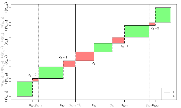
Figure 15: Exemplary situation in the proof of Theorem 4.9, part (ii), Case 1. ($F$ and $G$ are assumed to be standardized w.r.t. the mean.)

The only situation left to be considered is the one shown in the lower right panel of Figure 5, where $F$ and $G$ intersect multiple times. The structure of those intersections can be further narrowed down before then being divided in three cases in the proof. The line of reasoning in Case 1 is illustrated in Figure 15. The main focus lies on the ratio between the two areas between each pair of vertical lines. If the left area is divided by the right area, the resulting ratio decreases as the corresponding index ($c_{0}-2,c_{0}-1,c_{0},\ldots$) increases. (In the proof, the ratio for an index $c$ is denoted by $m(c)$.) Now, $t_{0}$ is chosen such that this ratio is smaller than $1$ on the left side of $t_{0}$ and larger than or equal to $1$ on the right side of $t_{0}$. In Figure 15, the smaller area of each pair is filled in red and the larger one is filled in green. For all $t\geq t_{0}$, the sum of the green areas on the right side of $t$ minus the sum of the red areas on the right side of $t$ is required to be non-negative. For $t=t_{0}$, this is obviously true since the ratio between the green and the red areas is no smaller than $1$ for each index. If $t$ is increased from $t_{0}$ towards $\infty$, the red areas are always reduced before the corresponding green areas are. The situation on the left side of $t_{0}$, so for $t\leq t_{0}$, is analogous.

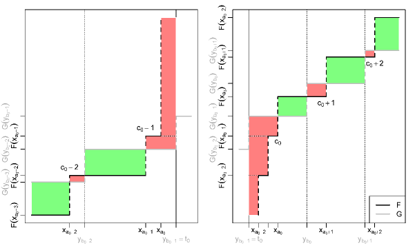
Figure 16: Exemplary situation in the proof of Theorem 4.9, part (ii), Cases 2 and 3, if $t_{0}=y_{b_{0}-1}$ was chosen instead of $t_{0}=x_{a_{0}-1}$ and $t_{0}=x_{a_{0}}$. ($F$ and $G$ are assumed to be standardized w.r.t. the mean.)

This begs the question why Cases 2 and 3 in part (ii) of the proof of Theorem 4.9 need to be considered separately and cannot be included in the line of reasoning illustrated by Figure 15. This is illustrated in Figure 16, where the left panel is exemplary for Case 2 (as the chain of intersections of $F$ and $G$ ends at index $c_{0}$, which is chosen as before) and the right panel is exemplary for Case 3 (as the chain of intersections of $F$ and $G$ begins at index $c_{0}$). In Case 3, if $t_{0}=y_{b_{0}-1}$ is chosen as before, it is possible for $F$ to exhibit more steep jumps on the right side of $t_{0}$, thus expanding the corresponding red area to be larger than the corresponding green area. This is possible because the chain of intersections of $F$ and $G$ ends at index $c_{0}$ and does not extend any further below that index. The problem can be solved by choosing $t_{0}=x_{a_{0}}$ instead. On the left side of $t_{0}$, $F$ is then smaller than $G$; on the right side of $t_{0}$, there is an additional green area before the first full pair of red and green areas, once again ensuring the non-negativity required in (37). The line of reasoning in Case 2 is analogous, just going down instead of up.

A.3 Proofs for Section 5

Proof of Theorem 5.4.

We prove this by constructing a counterexample for arbitrary values of $\alpha$ and $\beta$. First, define $n=\left\lfloor\frac{\beta-\alpha}{\min(\alpha,1-\beta)}\right\rfloor+1\in\mathbb{N}$ and choose $\delta\in\left(\frac{\beta-\alpha}{n},\min(\alpha,1-\beta)\right)\subseteq(0,1)$. The latter interval is not empty since

$$n>\frac{\beta-\alpha}{\min(\alpha,1-\beta)}\Leftrightarrow\min(\alpha,1-\beta)>\frac{\beta-\alpha}{n}$$

holds. Note that, by definition, $0\leq(n-1)\delta<\beta-\alpha<n\delta<1$ is true. The last inequality specifically follows from

$$n\delta <\left(\left\lfloor\frac{\beta-\alpha}{\min(\alpha,1-\beta)}\right\rfloor+1\right)\cdot\min(\alpha,1-\beta)$$

$$<(\beta-\alpha)+\min(\alpha,1-\beta)=1-\max(\alpha,1-\beta)<1.$$

Further, let $\varepsilon_{p}=\frac{(\beta-\alpha)-(n-1)\delta}{2}>0$, $\varepsilon_{q}=\frac{n\delta-(\beta-\alpha)}{2}>0$. Now we define $F,G\in\mathcal{D}_{0}$ by $F\;\hat{=}\;(A,(x_{j},p_{j})_{j\in A})$ and $G\;\hat{=}\;(B,(y_{j},q_{j})_{j\in B})$, where $A=\{1,\ldots,n+1\}$ with $x_{a}=a$ for all $a\in A$ and $B=\{1,\ldots,n+2\}$ with $y_{b}=b$ for all $b\in B$. Furthermore, let

$$p_{1} =\alpha+\varepsilon_{p},\quad p_{j} =\delta\ \forall j\in\{2,\ldots,n\},\quad p_{n+1} =(1-\beta)+\varepsilon_{p},$$

$$q_{1} =\alpha-\varepsilon_{q},\quad q_{j} =\delta\ \forall j\in\{2,\ldots,n+1\},\quad q_{n+2} =(1-\beta)-\varepsilon_{q}.$$

For all $j\in\{1,\ldots,n\}$, it holds that

$$G(y_{j}) =\alpha-\varepsilon_{q}+(j-1)\delta=\frac{\alpha+\beta}{2}+\delta\left(j-1-\frac{n}{2}\right)$$

$$<\frac{\alpha+\beta}{2}+\delta\left(j-\frac{n}{2}-\frac{1}{2}\right)=\alpha+\varepsilon_{p}+(j-1)\delta=F(x_{j})$$

$$<\frac{\alpha+\beta}{2}+\delta\left(j-\frac{n}{2}\right)=\alpha+\varepsilon_{p}+j\delta=G(y_{j+1}),$$

yielding $R(\leftrightharpoons)=\bigcup_{j=1}^{n+1}\{(j,j),(j,j+1)\}$. Hence, $F\leq_{\text{D-pm}}^{\text{disc}}G$. Since $F$ and $G$ are both lattice distributions with the same defining distance, it follows that $F\leq_{\text{disp}}^{\land\text{-disc}}G$. However,

$$\mathrm{IQR}({\alpha},{\beta})(F)=(n+1)-1=n>n-1=(n+1)-2=\mathrm{IQR}({\alpha},{\beta})(G).$$

Proof of Theorem 5.5.

Without restriction, let $F^{-1}(\frac{1}{2})=G^{-1}(\frac{1}{2})=0$. Furthermore, let $a_{0}\in A$ and $b_{0}\in B$ be the unique indices that satisfy $x_{a_{0}}=F^{-1}(\frac{1}{2})=0=G^{-1}(\frac{1}{2})=y_{b_{0}}$. Because of $F(x_{a_{0}-1})<\frac{1}{2}\leq G(y_{b_{0}})$ and $G(y_{b_{0}-1})<\frac{1}{2}\leq F(x_{a_{0}})$, $a_{0}\leftrightharpoons b_{0}$ holds. Hence, $F(x_{a_{0}})-F(x_{a_{0}-1})=p_{a_{0}}\geq q_{b_{0}}=G(y_{b_{0}})-G(y_{b_{0}-1})$ and it follows that $G(y_{b_{0}})\leq F(x_{a_{0}})$ or $G(y_{b_{0}-1})\geq F(x_{a_{0}-1})$.

We begin by assuming $G(y_{b_{0}})\leq F(x_{a_{0}})$ and show that, consequently, $y_{\beta}\geq x_{\alpha}$ holds for all pairs $(\alpha,\beta)\in R(\leftrightharpoons)$ higher than $(a_{0},b_{0})$. Choosing $G(y_{b_{k}-1})=\min\operatorname{NN}_{F}^{G}(a_{0}+k)$ for all $k\in\mathbb{N}$ such that $a_{0}+k\in A$ gives pairwise distinct indices $b_{k}\in\underline{B}$ such that $a_{0}+k\leftrightharpoons_{\land}b_{k}$. This is guaranteed by Lemma 3.16. Note that, for all $k\in\mathbb{N}$, $b_{k}$ is also the smallest index in $B$ such that $a_{0}+k\leftrightharpoons b_{k}$. Note also that $b_{0}<b_{1}$. Hence, for all pairs $(\alpha,\beta)\in R(\leftrightharpoons)$ higher than (or equal to) $(a_{0},b_{0})$, there exists a $k\in\mathbb{N}_{0}$ such that

$$x_{\alpha} =x_{a_{0}+k}=x_{a_{0}}+\sum_{j=1}^{k}(x_{a_{0}+j}-x_{a_{0}+j-1})=\sum_{j=1}^{k}(x_{a_{0}+j}-x_{a_{0}+j-1})$$

$$\leq\sum_{j=1}^{k}(y_{b_{j}}-y_{b_{j-1}})=y_{b_{0}}+\sum_{j=1}^{k}(y_{b_{j}}-y_{b_{j-1}})\leq y_{b_{k}}\leq y_{\beta}.$$

Analogously, the assumption $G(y_{b_{0}-1})\geq F(x_{a_{0}-1})$ yields $y_{\beta}\leq x_{\alpha}$ holds for all pairs $(\alpha,\beta)\in R(\leftrightharpoons)$ lower than $(a_{0},b_{0})$. With this in mind, we prove the assertion via case distinction.

1. $F(x_{a_{0}-1})\leq G(y_{b_{0}-1})<G(y_{b_{0}})\leq F(x_{a_{0}})$
   It holds that

   $$\mathrm{MDMAD}(G)-\mathrm{MDMAD}(F) =\sum_{(a,b)\in R(\leftrightharpoons)}r_{(a,b)}(|y_{b}-y_{b_{0}}|-|x_{a}-x_{a_{0}}|)$$

   $$=\sum_{(a,b)\in R(\leftrightharpoons)}r_{(a,b)}(|y_{b}|-|x_{a}|)$$

   $$=\sum_{\begin{subarray}{c}(a,b)\in R(\leftrightharpoons)\\ \text{lower than}(a_{0},b_{0})\end{subarray}}r_{(a,b)}(x_{a}-y_{b})$$

   $$\phantom{=}\;+\sum_{\begin{subarray}{c}(a,b)\in R(\leftrightharpoons)\\ \text{higher than}(a_{0},b_{0})\end{subarray}}r_{(a,b)}(y_{b}-x_{a}).$$ (40)

   Since $x_{a}\geq y_{b}$ holds for all pairs $(a,b)\in R(\leftrightharpoons)$ lower than $(a_{0},b_{0})$ and $y_{b}\geq x_{a}$ holds for all pairs $(a,b)\in R(\leftrightharpoons)$ higher than $(a_{0},b_{0})$, (40) is non-negative. Thus, the proof in this case is completed.

2. $F(x_{a_{0}-1})<G(y_{b_{0}-1})<F(x_{a_{0}})<G(y_{b_{0}})$
   We start out by considering pairs $(a,b)\in R(\leftrightharpoons)$ that are higher than $(a_{0},b_{0})$. According to (15), $x_{a}>y_{b}$ is only possible for any such pair, if $a-a_{0}=b-b_{0}+1$ holds. Hence, let $(a,b)\in R(\leftrightharpoons)$ be higher than $(a_{0},b_{0})$ and satisfy $a-a_{0}=b-b_{0}+1$. Part 2 of the proof of Theorem 4.7 states that, in this case, the values of $F$ and $G$ alternate for index pairs between $(a_{0},b_{0})$ and $(a,b)$. In that area, the pairs in $R(\leftrightharpoons)$ are of the form

   $$(a_{0},b_{0}),(a_{0}+1,b_{0}),(a_{0}+1,b_{0}+1),(a_{0}+2,b_{0}+1),\ldots$$

   $$\ldots,(a-2,b-1),(a-1,b-1),(a-1,b),(a,b)$$ . (41)

   Hence,

   $$\;\sum_{\begin{subarray}{c}(a,b)\in R(\leftrightharpoons)\\ \text{higher than}(a_{0},b_{0})\end{subarray}}r_{(a,b)}(y_{b}-x_{a})$$

   $$\geq \;-\sum_{\begin{subarray}{c}c\in\mathbb{N}_{0}:\\ (a_{0}+1+c,b_{0}+c)\in R(\leftrightharpoons)\end{subarray}}r_{(a_{0}+1+c,b_{0}+c)}(x_{a_{0}+1+c}-y_{b_{0}+c})$$

   $$= \;-\sum_{\begin{subarray}{c}c\in\mathbb{N}_{0}:\\ F(x_{a_{0}+c})<G(y_{b_{0}+c})\end{subarray}}(G(y_{b_{0}+c})-F(x_{a_{0}+c}))(x_{a_{0}+1+c}-y_{b_{0}+c}).$$ (42)

   Note that, due to the structure of $R(\leftrightharpoons)$ given in (41), $F(x_{a_{0}+c})<G(y_{b_{0}+c})$ is equivalent to $(a_{0}+1+c,b_{0}+c)\in R(\leftrightharpoons)$ for any $c\in\mathbb{N}_{0}$. Since $(a_{0}+1+c)-(a_{0}+1)<(b_{0}+c)-b_{0}+1$ holds for all $c\in\mathbb{N}_{0}$ such that $(a_{0}+1+c,b_{0}+c)\in R(\leftrightharpoons)$, (15) implies $x_{a_{0}+1+c}-y_{b_{0}+c}\leq x_{a_{0}+1}-y_{b_{0}}$. Combined with (42), this yields

   $$\sum_{\begin{subarray}{c}(a,b)\in R(\leftrightharpoons)\\ \text{higher than}(a_{0},b_{0})\end{subarray}}r_{(a,b)}(y_{b}-x_{a})\geq-(x_{a_{0}+1}-y_{b_{0}})\cdot\sum_{\begin{subarray}{c}c\in\mathbb{N}_{0}:\\ F(x_{a_{0}+c})<G(y_{b_{0}+c})\end{subarray}}(G(y_{b_{0}+c})-F(x_{a_{0}+c})).$$ (43)

   For any $c\in\mathbb{N}_{0}$ with $F(x_{a_{0}+c})<G(y_{b_{0}+c})$ and $F(x_{a_{0}+c+1})<G(y_{b_{0}+c+1})$, it can be shown analogously to (32) that

   $$\frac{G(y_{b_{0}+c+1})-F(x_{a_{0}+c+1})}{F(x_{a_{0}+c+2})-F(x_{a_{0}+c+1})}\leq\frac{G(y_{b_{0}+c})-F(x_{a_{0}+c})}{F(x_{a_{0}+c+1})-F(x_{a_{0}+c})}.$$

   By applying this inequality recursively, we obtain

   $$\frac{G(y_{b_{0}})-F(x_{a_{0}})}{F(x_{a_{0}+1})-F(x_{a_{0}})}\geq\frac{G(y_{b_{0}+c})-F(x_{a_{0}+c})}{F(x_{a_{0}+c+1})-F(x_{a_{0}+c})}$$

   for all $c\in\mathbb{N}_{0}$ with $F(x_{a_{0}+c})<G(y_{b_{0}+c})$. With this, we can continue inequality (43) by writing

   $$\;\sum_{\begin{subarray}{c}(a,b)\in R(\leftrightharpoons)\\ \text{higher than}(a_{0},b_{0})\end{subarray}}r_{(a,b)}(y_{b}-x_{a})$$

   $$\geq \;-(x_{a_{0}+1}-y_{b_{0}})\cdot\sum_{\begin{subarray}{c}c\in\mathbb{N}_{0}:\\ F(x_{a_{0}+c})<G(y_{b_{0}+c})\end{subarray}}(G(y_{b_{0}+c})-F(x_{a_{0}+c}))$$

   $$= \;-(x_{a_{0}+1}-y_{b_{0}})\cdot\sum_{\begin{subarray}{c}c\in\mathbb{N}_{0}:\\ F(x_{a_{0}+c})<G(y_{b_{0}+c})\end{subarray}}\bigg{(}\frac{G(y_{b_{0}+c})-F(x_{a_{0}+c})}{F(x_{a_{0}+c+1})-F(x_{a_{0}+c})}\cdot$$

   $$\;\phantom{-(x_{a_{0}+1}-y_{b_{0}})\cdot\sum_{\begin{subarray}{c}c\in\mathbb{N}_{0}:\\ F(x_{a_{0}+c})<G(y_{b_{0}+c})\end{subarray}}}\qquad(F(x_{a_{0}+c+1})-F(x_{a_{0}+c}))\bigg{)}$$

   $$\geq \;-(x_{a_{0}+1}-y_{b_{0}})\cdot\frac{G(y_{b_{0}})-F(x_{a_{0}})}{F(x_{a_{0}+1})-F(x_{a_{0}})}\sum_{\begin{subarray}{c}c\geq 0\\ F(x_{a_{0}+c})<G(y_{b_{0}+c})\end{subarray}}(F(x_{a_{0}+c+1})-F(x_{a_{0}+c}))$$

   $$\geq \;-(x_{a_{0}+1}-y_{b_{0}})\cdot\frac{G(y_{b_{0}})-F(x_{a_{0}})}{F(x_{a_{0}+1})-F(x_{a_{0}})}\cdot(1-F(x_{a_{0}}))$$

   $$\geq \;-\frac{x_{a_{0}+1}-y_{b_{0}}}{2}\cdot\frac{G(y_{b_{0}})-F(x_{a_{0}})}{F(x_{a_{0}+1})-F(x_{a_{0}})}.$$ (44)

   Now we consider the pairs $(a,b)\in R(\leftrightharpoons)$ lower than $(a_{0},b_{0})$. According to (15), $x_{a}-y_{b}<x_{a_{0}+1}-y_{b_{0}}$ is only possible for this kind of pair if $a_{0}-a=b_{0}-b$ holds. In this case, the values of $F$ and $G$ between these pairs of indices once again alternate so that the corresponding elements of $R(\leftrightharpoons)$ are of the form

   $$(a_{0},b_{0}),(a_{0},b_{0}-1),(a_{0}-1,b_{0}-1),(a_{0}-1,b_{0}-2),\ldots$$

   $$\ldots,(a+2,b+1),(a+1,b+1),(a+1,b),(a,b)$$ .

   It follows

   $$\;\sum_{\begin{subarray}{c}(a,b)\in R(\leftrightharpoons)\\ \text{lower than}(a_{0},b_{0})\end{subarray}}r_{(a,b)}(x_{a}-y_{b})$$

   $$\geq \;(x_{a_{0}+1}-y_{b_{0}})\cdot\Bigg{(}F(x_{a_{0}})-\sum_{\begin{subarray}{c}c\in\mathbb{N}_{0}:\\ (a_{0}-c,b_{0}-c)\in R(\leftrightharpoons)\end{subarray}}r_{(a_{0}-c,b_{0}-c)}\Bigg{)}$$

   $$= \;(x_{a_{0}+1}-y_{b_{0}})\cdot\Bigg{(}F(x_{a_{0}})-\sum_{\begin{subarray}{c}c\in\mathbb{N}_{0}:\\ F(x_{a_{0}-c})>G(y_{b_{0}-c-1})\end{subarray}}(F(x_{a_{0}-c})-G(y_{b_{0}-c-1}))\Bigg{)}.$$ (45)

   Note for the inequality that $x_{a}-y_{b}<0=x_{a_{0}}-y_{b_{0}}$ would imply $a_{0}-a=b_{0}-b+1$, which contradicts $a_{0}-a=b_{0}-b$. For any $c\in\mathbb{N}_{0}$ with $F(x_{a_{0}-c})>G(y_{b_{0}-c-1})$ and $F(x_{a_{0}-c-1})>G(y_{b_{0}-c-2})$, one can now again show similarly to (32) that

   $$\frac{F(x_{a_{0}-c})-G(y_{b_{0}-c-1})}{F(x_{a_{0}-c})-F(x_{a_{0}-c-1})}\geq\frac{F(x_{a_{0}-c-1})-G(y_{b_{0}-c-2})}{F(x_{a_{0}-c-1})-F(x_{a_{0}-c-2})}$$

   holds. Inductively, it follows that

   $$\frac{F(x_{a_{0}})-G(y_{b_{0}-1})}{F(x_{a_{0}})-F(x_{a_{0}-1})}\geq\frac{F(x_{a_{0}-c})-G(y_{b_{0}-c-1})}{F(x_{a_{0}-c})-F(x_{a_{0}-c-1})}$$

   is true for all $c\in\mathbb{N}_{0}$ with $F(x_{a_{0}-c})>G(y_{b_{0}-c-1})$. Continuing from (45), we obtain

   $$\;\sum_{\begin{subarray}{c}(a,b)\in R(\leftrightharpoons)\\ \text{lower than}(a_{0},b_{0})\end{subarray}}r_{(a,b)}(x_{a}-y_{b})$$

   $$\geq \;(x_{a_{0}+1}-y_{b_{0}})\cdot\Bigg{(}F(x_{a_{0}})-\sum_{\begin{subarray}{c}c\in\mathbb{N}_{0}:\\ F(x_{a_{0}-c})>G(y_{b_{0}-c-1})\end{subarray}}\bigg{(}\frac{F(x_{a_{0}-c})-G(y_{b_{0}-c-1})}{F(x_{a_{0}-c})-F(x_{a_{0}-c-1})}\cdot$$

   $$\;\phantom{(x_{a_{0}+1}-y_{b_{0}})\cdot\Bigg{(}F(x_{a_{0}})-\sum_{\begin{subarray}{c}c\geq 0\\ F(x_{a_{0}-c})>G(y_{b_{0}-c-1})\end{subarray}}}\quad(F(x_{a_{0}-c})-F(x_{a_{0}-c-1}))\bigg{)}\Bigg{)}$$

   $$\geq \;(x_{a_{0}+1}-y_{b_{0}})\cdot\Bigg{(}F(x_{a_{0}})-\frac{F(x_{a_{0}})-G(y_{b_{0}-1})}{F(x_{a_{0}})-F(x_{a_{0}-1})}\cdot$$

   $$\;\phantom{(x_{a_{0}+1}-y_{b_{0}})\cdot\bigg{(}F(x_{a_{0}})-}\sum_{\begin{subarray}{c}c\in\mathbb{N}_{0}:\\ F(x_{a_{0}-c})>G(y_{b_{0}-c-1})\end{subarray}}\quad(F(x_{a_{0}-c})-F(x_{a_{0}-c-1}))\Bigg{)}$$

   $$\geq \;(x_{a_{0}+1}-y_{b_{0}})\cdot\left(F(x_{a_{0}})-\frac{F(x_{a_{0}})-G(y_{b_{0}-1})}{F(x_{a_{0}})-F(x_{a_{0}-1})}\cdot F(x_{a_{0}})\right)$$

   $$\geq \;\frac{x_{a_{0}+1}-y_{b_{0}}}{2}\cdot\left(1-\frac{F(x_{a_{0}})-G(y_{b_{0}-1})}{F(x_{a_{0}})-F(x_{a_{0}-1})}\right).$$ (46)

   Now, by combining (40), which is also valid in Case 2, with (44) and (46), it follows that

   $$\;\mathrm{MDMAD}(G)-\mathrm{MDMAD}(F)$$

   $$\geq \;\frac{x_{a_{0}+1}-y_{b_{0}}}{2}\cdot\left(1-\frac{G(y_{b_{0}})-F(x_{a_{0}})}{F(x_{a_{0}+1})-F(x_{a_{0}})}-\frac{F(x_{a_{0}})-G(y_{b_{0}-1})}{F(x_{a_{0}})-F(x_{a_{0}-1})}\right)$$

   $$\geq \;\frac{x_{a_{0}+1}-y_{b_{0}}}{2}\cdot\left(1-\frac{q_{b_{0}}}{\min\{p_{a_{0}},p_{a_{0}+1}\}}\right)\geq 0,$$

   where the last inequality holds since $(a_{0},b_{0}),(a_{0}+1,b_{0})\in R(\leftrightharpoons)$ is true by assumption.

3. $G(y_{b_{0}-1})<F(x_{a_{0}-1})<G(y_{b_{0}})<F(x_{a_{0}})$
   This case is completely analogous to Case 2 for reasons of symmetry.

A.4 Proofs for Section 6

Proof of Theorem 6.3.

Let $\lambda=1-\pi_{G}\in(0,1)$ and $\varrho=\frac{\log(1-\pi_{F})}{\log(1-\pi_{G})}>1$, then $\pi_{F}=1-\lambda^{\varrho}$ and $\pi_{G}=1-\lambda$. Note that $F\leq_{\text{D-supp}}^{\land\text{-disc}}G$ holds because both are lattice distributions with defining distance $1$. We start by finding an equivalent condition for $(a,b)\in R(\leftrightharpoons)$, where $a,b\in\mathbb{N}=A=B$. The statement $(a,b)\in R(\leftrightharpoons)$ is equivalent to $F(a-1)<G(b)$ and $G(b-1)<F(a)$ holding simultaneously. For these two inequalities, the following equivalences hold:

$$F(a-1)<G(b) \Leftrightarrow 1-\lambda^{\varrho(a-1)}<1-\lambda^{b}\Leftrightarrow\lambda^{\varrho(a-1)}>\lambda^{b}\Leftrightarrow\varrho(a-1)<b\Leftrightarrow a<\tfrac{b}{\varrho}+1,$$

$$G(b-1)<F(a) \Leftrightarrow 1-\lambda^{b-1}<1-\lambda^{\varrho a}\Leftrightarrow\lambda^{b-1}>\lambda^{\varrho a}\Leftrightarrow b-1<\varrho a\Leftrightarrow a>\tfrac{b-1}{\varrho}.$$

Overall, $(a,b)\in R(\leftrightharpoons)$ is equivalent to $a\in(\frac{b-1}{\varrho},\frac{b}{\varrho}+1)$. Because $a$ is required to be a natural number and $(\frac{b}{\varrho}+1)-\frac{b-1}{\varrho}=1+\frac{1}{\varrho}\in(1,2)$, there are either one or two possible values for $a$ for a fixed $b\in\mathbb{N}$. Particularly, it follows that

$$a\in\left\{\left\lfloor\frac{b}{\varrho}\right\rfloor+1,\left\lceil\frac{b-1}{\varrho}\right\rceil\right\}.$$

The two values are different, if there exists an $n\in\mathbb{N}$ such that $\frac{b-1}{\varrho}\leq n\leq\frac{b}{\varrho}$. We consider the two elements separately. To this end, note that

$$\lambda^{b-1}-\lambda^{b} =\mathbb{P}(Y=b)$$

$$\leq\mathbb{P}(X=a)=\lambda^{\varrho(a-1)}-\lambda^{\varrho a}\quad\forall(a,b)\in\bigcup_{b\in\mathbb{N}}\left\{\left(\left\lfloor\frac{b}{\varrho}\right\rfloor+1,b\right),\left(\left\lceil\frac{b-1}{\varrho}\right\rceil,b\right)\right\}$$

is equivalent to $F\leq_{\text{D-pm}}^{\text{disc}}G$, and therefore to $F\leq_{\text{disp}}^{\land\text{-disc}}G$.

1. Let $a=\left\lceil\frac{b-1}{\varrho}\right\rceil$.
   It holds that

   $$\lambda^{\varrho(a-1)}-\lambda^{\varrho a}=\lambda^{\varrho(a-1)}(1-\lambda^{\varrho})>\lambda^{\varrho\cdot\frac{b-1}{\varrho}}(1-\lambda^{\varrho})=\lambda^{b-1}-\lambda^{b-1+\varrho}>\lambda^{b-1}-\lambda^{b},$$

   where the last inequality is true because $\varrho>1$ implies $\lambda^{b-1+\varrho}<\lambda^{b}$.

2. Let $a=\left\lfloor\frac{b}{\varrho}\right\rfloor+1$.
   It holds that

   $$\lambda^{\varrho(a-1)}-\lambda^{\varrho a}=\lambda^{\varrho(a-1)}(1-\lambda^{\varrho})>\lambda^{\varrho\cdot\frac{b}{\varrho}}(1-\lambda^{\varrho})=\lambda^{b}(1-\lambda^{\varrho}).$$

   Thus, it is sufficient to show

   $$\lambda^{b-1}(\lambda-\lambda^{\varrho+1})\geq\lambda^{b-1}-\lambda^{b}$$

   or, equivalently,

   $$2\lambda\geq\lambda^{\varrho+1}+1.$$

   This, in turn, is equivalent to

   $$\lambda(2-\lambda^{\varrho})\geq 1 \Leftrightarrow\lambda^{\varrho}\leq 2-\tfrac{1}{\lambda}$$

   $$\Leftrightarrow\varrho\geq\frac{\log(2-\tfrac{1}{\lambda})}{\log(\lambda)}=\frac{\log(2\lambda-1)}{\log(\lambda)}-1,$$

   which is true by assumption.

References

- [1] Fabio Bellini “Isotonicity Results for Generalized Quantiles” In Statistics & Probability Letters 82, 2012, pp. 2017–2024
- [2] Fabio Bellini, Lorenzo Mercuri and Edit Rroji “Implicit Expectiles and Measures of Implied Volatility” In Quantitative Finance 18, 2018, pp. 1851–1864
- [3] Peter J. Bickel and Erich L. Lehmann “Descriptive Statistics for Nonparametric Models. III. Dispersion” In The Annals of Statistics 4, 1976, pp. 1139–1158
- [4] Peter J. Bickel and Erich L. Lehmann “Descriptive Statistics for Nonparametric Models. IV. Spread” In Contributions to Statistics. Jaroslav Hajek Memorial Volume D. Reidel Pub. Co., 1979, pp. 33–40
- [5] Andreas Eberl and Bernhard Klar “On the Skewness Order of van Zwet and Oja” In Mathematical Methods of Statistics 28, 2019, pp. 262–278
- [6] Andreas Eberl and Bernhard Klar “A Note on a Measure of Asymmetry” In Statistical Papers 62, 2021, pp. 1483–1497
- [7] Andreas Eberl and Bernhard Klar “Stochastic Orders and Measures of Skewness and Dispersion Based on Expectiles” In Statistical Papers, 2022 DOI: 10.1007/s00362-022-01331-x
- [8] Andreas Eberl and Bernhard Klar “Measures of kurtosis – inadmissible for asymmetric distributions?” Submitted, 2023+
- [9] Alessandra Giovagnoli and H. P. Wynn “Multivariate Dispersion Orderings” In Statistics & Probability Letters 22, 1995, pp. 325–332
- [10] Werner Hürlimann “On Risk And Price: Stochastic Orderings And Measures” In Transactions of the 27th International Congress of Actuaries, 2002
- [11] Michael Kourkoulos and Constantinos Tzanakis “History, and Students’ Understanding of Variance In Statistics” In BSHM Bulletin 25, 2010, pp. 168–178
- [12] Tommaso Lando, Idir Arab and Paulo Eduardo Oliveira “Transform Orders and Stochastic Monotonicity of Statistical Functionals” Early view In Scandinavian Journal of Statistics, 2022 DOI: 10.1111/sjos.12629
- [13] Alfred Müller and Dietrich Stoyan “Comparison Methods for Stochastic Models and Risks”, Wiley Series in Probability and Statistics Chichester: Wiley, 2002
- [14] Hannu Oja “On Location, Scale, Skewness and Kurtosis of Univariate Distributions” In Scandinavian Journal of Statistics 8, 1981, pp. 154–168
- [15] Héctor M. Ramos and Miguel A. Sordo “Dispersion Measures and Dispersive Orderings” In Statistics & Probability Letters 861, 2003, pp. 123–131
- [16] Miguel A. Sordo, Marilia C. Souza and Alfonso Suárez-Llorens “Testing Variability Orderings by Using Gini’s Mean Differences” In Statistical Methodology 32, 2016, pp. 63–76
- [17] W. R. Zwet “Convex Transformations of Random Variables”, 1964