Cosmological dynamics of interacting dark energy and dark matter in $f(Q)$ gravity

Abstract

In this work, we explore the behavior of interacting dark energy and dark matter within a model of $f(Q)$ gravity, employing a standard framework of dynamical system analysis. We consider the power-law $f(Q)$ model incorporating with two different forms of interacting dark energy and dark matter: $3\alpha H\rho_{m}$ and $\frac{\alpha}{3H}\rho_{m}\rho_{DE}$. The evolution of $\Omega_{m}$, $\Omega_{r}$, $\Omega_{DE}$, $q$, and $\omega$ for different values of the model parameter $n$ and the interaction parameter $\alpha$ has been examined. Our results show that the universe was dominated by matter in the early stages and will be dominated by dark energy in later stages. Using the observational data, the fixed points are found to be stable and can be represented the de Sitter and quintessence acceleration solutions. We discover that the dynamical profiles of the universe in $f(Q)$ dark energy models are influenced by both the interaction term and the relevant model parameters.

Keywords: $f(Q)$ Gravity; Dark Energy; Dark Matter; Dynamical Analysis

I Introduction

Observational data has confirmed that the universe has entered a period of accelerated expansion. This evidence comes from various independent sources, including Supernovae Type Ia (SNe Ia) [1, 2, 3], temperature anisotropies in the Cosmic Microwave Background (CMB) observed by WMAP [4, 5], and Baryon Acoustic Oscillations [6, 7]. According to the framework of general relativity (GR), this accelerated expansion is driven by a new energy density component with negative pressure, referred to as dark energy (DE). Despite its crucial role, little is known about DE. Understanding the origin of DE, which causes the current cosmic acceleration, remains one of the major unresolved issues in modern cosmology. The standard equation of state $\omega=p/\rho$, where $\omega\geq 0$, cannot explain this phase of cosmic acceleration. Instead, an unknown component with negative pressure, characterized by $\omega<-\tfrac{1}{3}$, is necessary to describe the universe’s acceleration. However, the exact nature of DE is still a mystery. Numerous attempts have been made to address this significant problem, as discussed in Refs.[8, 9, 10, 11, 12, 13, 14, 15, 16, 17, 18, 19, 20, 21, 22]. The most straightforward candidate for dark energy is the cosmological constant, $\Lambda$. However, as pointed out in Ref.[23], the cosmological constant is vastly smaller than what is predicted by modern elementary particle theories. To differentiate between the cosmological constant and other potential sources of dark energy that change over time, researchers use dynamical models to study the evolution of the equation of state of DE. Therefore, a mechanism must be identified to achieve a small value of $\Lambda$ that aligns with observations.

It is well established that the pure cosmological constant cannot explain the accelerated expansion of the early universe, as it cannot connect to the radiation-dominated era. An alternative and compelling candidate for both dark energy and inflation is a scalar field with a slowly varying potential. In the realm of dark energy, numerous scalar field models have been proposed, including quintessence [24, 25, 26, 27, 28, 29] and k-essence [30, 31, 32, 33] scenarios. These models predict various behaviors for the equation of state of dark energy. However, current observational data cannot distinguish these models from the $\Lambda$-cold-dark-matter ($\Lambda$CDM) model. Moreover, achieving viable scalar-field models within the framework of particle physics is challenging due to the extremely small scalar mass required for present-day cosmic acceleration [34, 35]. Another approach to explaining the universe’s accelerated expansion involves dynamical dark energy models based on modifying gravity over large distances. Examples of such models include $f(R)$ gravity, where the Ricci scalar is replaced by a more general function, $f(R)$ [36, 37, 38, 39], as well as scalar-tensor theories [40, 41, 42, 43, 44, 45], Galileon gravity [46], and Gauss-Bonnet gravity [47, 48]. For several decades, dynamical system analysis has been used in cosmology to qualitatively study these models, proving effective in identifying and classifying their asymptotic behaviors [49, 50]. Recently, this framework has been applied to investigate various dark energy models, including those based on $f(R)$ gravity [13, 51]. A series of papers [52, 54, 53, 55, 56, 57] has systematically analyzed $f(R)$ theories, identifying models that provide correct cosmological evolution from a vast number of possibilities. These analyses have led to the construction of cosmologically viable $f(R)$ gravity models, which feature appropriate trajectories in the dynamical system phase space and are compatible with local gravity constraints [20, 21, 55]. A notable advantage of these models is that they achieve cosmic acceleration without requiring a dark energy component. Furthermore, these models impose stringent constraints from local gravity tests and various observational data, making them more rigorous compared to modified matter models.

The authors of Refs.[58, 59, 60, 61, 62] initiated and expanded the phase space analysis of $f(R)$ gravity using the autonomous dynamical systems approach. While there has been considerable research on dynamical systems in $f(R)$ gravity involving non-interacting dark energy and dark matter [51], the study of interacting dark energy within the $f(R)$ gravity framework has received less attention, particularly in the context of dynamical system analysis [63, 64, 65, 66, 67, 68]. Investigating interacting dark energy and dark matter is valuable for understanding the behavior of accelerated scaling solutions where the energy densities of dark energy ($\Omega_{DE}$) and dark matter ($\Omega_{DM}$) are approximately equal, and the universe is accelerating. This research could also elucidate the coupling between dark matter structure formation and the time evolution of dark energy, potentially explaining why dark energy dominates over dark matter in the late universe. Additionally, the impact of interacting dark energy models on the global 21cm signal was explored in Ref.[70], and some interacting dark energy models and their potential to cause future singularities have been analyzed in Ref.[71].

The purpose of this work is to investigate the interaction between dark energy and dark matter within viable models of $f(Q)$ gravity. The $f(Q)$ gravity theory [72, 73] is one of the most promising approaches to explaining the accelerated expansion of the universe, involving dynamical dark energy models that modify gravity at large distances. This theory extends the alternative to General Relativity known as the symmetric teleparallel theory, which is based on the nonmetricity scalar $Q$, with both curvature and torsion being absent. Geometrically, the nonmetricity $Q$ describes the variation in the length of a vector during parallel transport. $f(Q)$ gravity presents intriguing applications [74, 75, 76, 77, 78, 79] and easily satisfies the constraints from gravitational wave observations [80]. At cosmological scales, $f(Q)$ can create a gravitational interaction that reveals new and interesting patterns in both the background evolution [72, 73, 81, 82, 83, 84] and the propagation of scalar and tensor perturbations [73, 81, 74, 85, 86, 87]. Additionally, certain forms of the $f(Q)$ function have been shown to mitigate the $\sigma_{8}$ tension [88], while others provide a better fit to cosmological data [89, 90, 91, 92, 93, 94, 95, 96, 97]. This theory is thus challenging $\Lambda$CDM from different perspectives [98]. Furthermore, a dynamical system analysis of both background and perturbation equations is conducted in $f(Q)$ gravity to independently verify the validity of result [87, 99, 100, 101, 102, 103, 104].

The structure of this work is organized as follows: In Section II, we present the fundamental cosmological equations of the general $f(Q)$ theory and derive the Friedmann equation corresponding to the FLRW metric. In Section III, we derive the autonomous dynamical system within the framework of $f(Q)$ gravity theory, focusing on the interaction between dark energy and dark matter. In Section IV, we apply the power-law $f(Q)$ model to enclose the dynamical system and conduct a further study of $f(Q)$ gravity. Finally, we discuss our findings in Section V.

II Formulation of $f(Q)$ gravity theory

In this section, we briefly discuss the formulation of $f(Q)$ gravity, a simple generalization of symmetric teleparallel gravity theory. This theory requires a different curvature and torsion-free connection, i.e., it is wholly dependent on nonmetricity. This formulation introduces new dynamics compared to General Relativity (GR) by allowing the function $f(Q)$ to dictate how nonmetricity influences the gravitational interaction. The non-metricity tensor $Q_{\sigma\mu\nu}$ is defined as

$$Q_{\sigma\mu\nu}=\nabla_{\sigma}g_{\mu\nu},$$ (1)

which geometrically describes the variation of the length of a vector in the parallel transport.
With the aid of the nonmetricity tensor, we can define the superpotential tensor $P_{\,\,\mu\nu}^{\sigma}$ as

$$4P_{\,\,\mu\nu}^{\sigma}=-Q^{\sigma}_{\,\,\,\,\mu\nu}+2Q^{\,\,\,\,\,\,\sigma}_{(\mu\,\,\,\,\nu)}-Q^{\sigma}g_{\mu\nu}-\tilde{Q}^{\sigma}g_{\mu\nu}-\delta^{\sigma}_{(\mu}\,Q\,_{\nu)},$$ (2)

where $Q_{\sigma}=Q_{\sigma\,\,\,\,\mu}^{\,\,\,\,\mu}$ and $\tilde{Q}_{\sigma}=Q^{\mu}_{\,\,\,\,\sigma\mu}\,$.
From the above quantities, we can obtain a non-metricity scalar as

$$Q=-Q_{\sigma\mu\nu}P^{\sigma\mu\nu}.$$ (3)

The action for $f(Q)$ gravity [72]

$$S=\int\left[\frac{1}{2\kappa^{2}}f(Q)+\mathcal{L}_{m}\right]\sqrt{-g}\,d^{4}x,$$ (4)

where $f(Q)$ represents any function of the scalar $Q$, $g$ denotes the determinant of $g_{\mu\nu}$, and $\mathcal{L}_{m}$ stands for the matter Lagrangian density.
The equations of motion in $f(Q)$ gravity are derived by varying the action with respect to the metric and the connection. This leads to a set of modified field equations that incorporate the effects of nonmetricity, providing a richer structure for modeling gravitational phenomena, and it is written as

$$\frac{2}{\sqrt{-g}}\nabla_{\sigma}\left(f_{Q}\sqrt{-g}\,P^{\sigma}_{\,\,\mu\nu}\right)+\frac{1}{2}f(Q)\,g_{\mu\nu}\\ +f_{Q}\left(P_{\mu\sigma\lambda}Q_{\nu}^{\,\,\,\sigma\lambda}-2Q_{\sigma\lambda\mu}P^{\sigma\lambda}_{\,\,\,\,\,\,\nu}\right)=-T_{\mu\nu},$$ (5)

where $f_{Q}=\frac{df}{dQ}$. The energy-momentum tensor for matter is now defined as $T_{\mu\nu}\equiv-\frac{2}{\sqrt{-g}}\frac{\delta(\sqrt{-g})\mathcal{L}_{m}}{\delta g^{\mu\nu}}$.
To apply $f(Q)$ gravity in a cosmological context, we consider the spatially flat Friedmann-Lemaître-Robertson-Walker (FLRW) spacetime, characterized by the metric

$$ds^{2}=-dt^{2}+a^{2}(t)\,\delta_{ij}\,dx^{i}\,dx^{j},\,\,\,\,\,\,(i,j=1,2,3),$$ (6)

where $a(t)$ is the cosmological scale factor. For this metric, the corresponding nonmetricity scalar is given by $Q=6H^{2}$, with $H=\frac{\dot{a}}{a}$ representing the Hubble parameter and the dot denotes a derivative with respect to the coordinate time $t$. Applying the FLRW metric into the general field equation (5), the Friedman equations of $f(Q)$ cosmology read as

$$6H^{2}f_{Q}-\frac{f}{2} = \rho$$ (7)

$$\left(12H^{2}\,f_{QQ}+f_{Q}\right)\dot{H} = -\frac{1}{2}(p+\rho),$$ (8)

where $f_{Q}=\frac{df}{dQ}$, and $f_{QQ}=\frac{d^{2}f}{dQ^{2}}$.
To study the interaction between dark energy and dark matter, we have to modify the conservation equations of the dark energy and the matter given above by adding some coupling term $\mathcal{U}$ as [68]

$$\dot{\rho}_{DE}+3H(p_{DE}+\rho_{DE})=\mathcal{U}\,,$$

$$\dot{\rho}_{m}+3H\,\rho_{m}=-\mathcal{U}\,,$$

$$\dot{\rho}_{r}+4H\,\rho_{r}=0\,.$$

In addition, the coupling term $\mathcal{U}$ between dark energy and dark matter can be interpreted as the exchange rate of energy density between these two components. When $\mathcal{U}>0$, energy is transferred from dark matter to dark energy, whereas when $\mathcal{U}<0$, energy is transferred from dark energy to dark matter.

III Autonomous dynamical system of interacting dark energy and dark matter

In this section, we derive the autonomous dynamical system within the framework of $f(Q)$ gravity theory, focusing on the interaction between dark energy and dark matter. Our approach involves incorporating two interacting terms. The first term relies solely on the energy density of the matter sector, the Hubble parameter, and a coupling constant $\alpha$, structured multiplicatively as $\mathcal{U}=3\alpha\,H\,\rho_{m}$. The second term encompasses the multiplication of energy densities from both sectors, capturing the immediate effects of both dark matter and dark energy on the interaction term, with a dimensionless coupling constant $\alpha$, denoted as $\mathcal{U}=\frac{\alpha}{3H}\rho_{m}\,\rho_{de}$.
According to the Friedmann equation (7), we can define the dimensionless variable as

$$x=\frac{f}{12H^{2}\,F},\,\,\,\,\,y=\frac{\rho_{r}}{6H^{2}\,F}.$$ (9)

Invoking the above dimensionless variables, it is straightforward to derive the autonomous equations which play a key role for studying the dynamical system for the interacting dark energy and dark matter.

III.1 Case I : $\mathcal{U}=3\alpha\,H\,\rho_{m}$

Using Eq.(7), the autonomous dynamical system is given by

$$\frac{dx}{dN}=(1-x)\frac{\dot{H}}{H^{2}}+3x-3x^{2}+xy+3\alpha\,x(1-x-y),$$ (10)

$$\frac{dy}{dN}=-\frac{\dot{H}}{H^{2}}\,y-y+y^{2}-3xy+3\alpha\,y(1-x-y).$$ (11)

where the variable $N=ln\,a$ is e-folding number and leads to $\frac{d}{dN}=\frac{1}{H}\frac{d}{dt}$.

III.2 Case II : $\mathcal{U}=\frac{\alpha}{3H}\rho_{m}\,\rho_{de}$

For this particular case, the autonomous dynamical system is given by

$$\frac{dx}{dN}=(1-x)\frac{\dot{H}}{H^{2}}+3x-3x^{2}+xy+\alpha\,x^{2}(1-x-y),$$ (12)

$$\frac{dy}{dN}=-\frac{\dot{H}}{H^{2}}\,y-y+y^{2}-3xy+\alpha\,xy(1-x-y).$$ (13)

where the variable $N=ln\,a$ is e-folding number and leads to $\frac{d}{dN}=\frac{1}{H}\frac{d}{dt}$.
Furthermore, we obtain the generalized equation for $\frac{\dot{H}}{H^{2}}$ as

$$\frac{\dot{H}}{H^{2}}=\frac{-3f_{Q}(1-x+\frac{y}{3})}{2Qf_{QQ}+f_{Q}}.$$ (14)

Consequently, the density parameters for individual matter species can be linked to the dimensionless variables outlined in Eq. (9). These variables serve as a set of constraint equations:

$$\Omega_{m}=1-x-y,\,\,\,\,\,\,\,\Omega_{r}=y,\,\,\,\,\,\,\,\Omega_{DE}=x.$$ (15)

Finally, we define the equation of state and deceleration parameters corresponding to the dimensionless variables to check the appropriate acceleration expansion of the universe, that is

$$\omega=-1+\frac{2f_{Q}(1-x+\frac{y}{3})}{2Qf_{QQ}+f_{Q}}$$ (16)

and

$$q=-1+\frac{3f_{Q}(1-x+\frac{y}{3})}{2Qf_{QQ}+f_{Q}}.$$ (17)

Both $\omega$ and $q$ represent different aspects of cosmic evolution, each uniquely influencing the large-scale structure of the universe. Grasping the significance of these parameters is essential for studying the effects of dark energy across various stages of cosmic evolution. Moreover, these parameters aid in comparing and differentiating between various dark energy models, each employing distinct mechanisms to drive cosmic acceleration.

IV Model:- $f(Q)=6\gamma\,H_{0}^{2}\left(\frac{Q}{Q_{0}}\right)^{n}$

In the previous section, we derived autonomous dynamical systems, and our primary objective is to investigate and analyze them. To accomplish this goal, we will focus on the designated power-law $f(Q)$ model, which has the form $f(Q)=6\gamma\,H_{0}^{2}\left(\frac{Q}{Q_{0}}\right)^{n}$, where $\gamma$ and $n$ are free model parameters.
Corresponding to our power-law $f(Q)$ model, Eq. (14) can be simplified to obtain

$$\frac{\dot{H}}{H^{2}}=-\frac{3(1-x+\frac{1}{3}y)}{2n-1}.$$ (18)

Now, we will find the critical points and corresponding eigenvalues for both the dynamical systems. Studying the critical points and assessing their stability is crucial for a comprehensive understanding of critical aspects in cosmic evolution driven by dark energy and dark matter interactions, as explored within the scope of this study. The properties of the dynamical system depend on the values of the constants $\alpha$ and $n$.

IV.1 For case I

The fixed points $(x,y)$ of the general dynamical system are the following:

$$P_{1}\mathrel{\mathop{\mathchar 58\relax}}(1,0),\,\,\,\,P_{2}\mathrel{\mathop{\mathchar 58\relax}}\left(\frac{1}{2n},\frac{2n-1}{2n}\right),$$ (19)

$$P_{3}\mathrel{\mathop{\mathchar 58\relax}}\left(\frac{1}{2n+\alpha(2n-1)},0\right).$$ (20)

Furthermore, the corresponding eigenvalues for each fixed point are given by

$$P_{1}\mathrel{\mathop{\mathchar 58\relax}}\{-4,-3(\alpha+1)\},\,\,\,\,P_{2}\mathrel{\mathop{\mathchar 58\relax}}\{4,1-3\alpha\},$$ (21)

$$P_{3}\mathrel{\mathop{\mathchar 58\relax}}\{3(\alpha+1),3\alpha-1\}.$$ (22)

Let us now focus on the dynamics of each critical point and its features in the further subsections.

IV.1.1 $P_{1}$: the de Sitter fixed point

We start the discussion with the first fixed point. Here we have

$$P_{1}\mathrel{\mathop{\mathchar 58\relax}}(x,y)=(1,0).$$

This critical point is independent of both the model and coupling parameters. Corresponding to this fixed point, the matter density, dark energy density, and effective EoS parameters are

$$\Omega_{m}=0,\,\,\,\,\Omega_{DE}=1,\,\,\,\,\omega=-1.$$ (23)

At this point, both dark matter and radiation are absent, and the universe is dominated by dark energy. The equation of state (EoS) at this fixed point indicates that the universe is experiencing an accelerated expansion. To study the stability of this fixed point, we can analyze the eigenvalues of the Jacobian matrix, which describe the behavior of the fixed point. The eigenvalues for the fixed point $P_{1}$ read

$$\{-4,\,\,\,-3(\alpha+1)\}.$$ (24)

The stability behavior of this fixed point (which depends on $\alpha$) is obtained as:

• Stable node for $\alpha>-1$,

• Saddle for $\alpha<-1$,

• Non-hyperbolic for $\alpha=-1$.

IV.1.2 $P_{2}$: Non-metricity dominated fixed point

Next, for the second fixed point, we have

$$P_{2}\mathrel{\mathop{\mathchar 58\relax}}(x,y)=\left(\frac{1}{2n},\frac{2n-1}{2n}\right).$$

The characteristics of this critical point solely depend on the model parameter $n$. Corresponding to this fixed point, the matter density, dark energy density, and effective EoS parameters are obtained as

$$\Omega_{m}=0,\,\,\,\,\Omega_{DE}=\frac{1}{2n},\,\,\,\,\omega=-1+\frac{4}{3n}.$$ (25)

The conditions for an accelerating universe are $n<0$ or $n>2$. When $n<0$, the universe exhibits phantom-like behavior, i.e., $\omega<-1$. When $n>2$, the universe exhibits quintessence-like behavior, i.e., $-1<\omega<-1/3$. In this fixed-point solution, a matter-dominated era occurs for $n=4/3$ and a radiation-dominated era for $n=1$. The eigenvalues for the fixed point $P_{2}$ are as follows:

$$\{4,\,\,\,1-3\alpha\}.$$ (26)

The stability behavior for this particular fixed point can be obtained for different $\alpha$, given by

• Saddle node for $\alpha>1/3$,

• Unstable for $\alpha<1/3$,

• Non-hyperbolic for $\alpha=1/3$.

IV.1.3 $P_{3}$: scaling solution fixed point

It is worth noting that our result modifies the scaling solution of $f(Q)$ gravity with the interacting dark energy parameter $\alpha$. The fixed point $P_{3}$ reads

$$P_{3}\mathrel{\mathop{\mathchar 58\relax}}(x,y)=\left(\frac{1}{2n+\alpha(2n-1)},0\right).$$

The properties of this critical point are influenced by both the model parameter $n$ and the coupling parameter $\alpha$. Corresponding to this fixed point, the matter density, dark energy density, and effective EoS parameters read as

$$\Omega_{m}=\frac{1}{\alpha-2(\alpha+1)n}+1,\,\,\,\,\Omega_{DE}=\frac{1}{2n+\alpha(2n-1)},$$

and

$$\omega=\frac{3\alpha-2(\alpha+1)n+2}{2(\alpha+1)n-\alpha}.$$

The conditions for an accelerating universe are shown in Fig. 1.

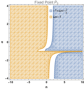
Figure 1: In this figure, we show the relationship between the model parameter $n$ and the interacting parameter $\alpha$ for the accelerating universe. The light blue region represents the quintessence-like behavior of an accelerating universe (i.e., $-1<\omega<-1/3$), while the golden region represents the phantom-like behavior of an accelerating universe (i.e., $\omega<-1$).

In this fixed point solution, we obtained a matter-dominated era for $n=\frac{3\alpha+2}{2(\alpha+1)}$, $1+\alpha\neq 0$, and radiation-dominated era for $n=\frac{5\alpha+3}{4(\alpha+1)}$, $1+\alpha\neq 0$.
The eigenvalues for the fixed point $P_{3}$ read as

$$\{3(\alpha+1),\,\,3\alpha-1\}.$$ (27)

We determine the stability of this fixed point for various ranges of $\alpha$. The ranges are as follows:

• Stable node for $\alpha<-1$

• Saddle for $-1<\alpha<1/3$

• Unstable node for $\alpha>1/3$.

In Figs. 2 and 3, we illustrate the evolution of $\Omega_{m}$, $\Omega_{r}$, $\Omega_{DE}$, $q$, and $\omega$ for different values of the model parameter $n$ and the interaction parameter $\alpha$. This is done using the numerical solution of the dynamical system with the initial conditions $x(0)=0.7$ and $y(0)=0.00005$. The motivation behind the choice of initial conditions is as follows: $x$ represents the dark energy density, which currently has a value of $0.7$. Similarly, $y$ represents the radiation density, which currently has a value of $0.00005$.

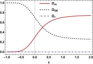
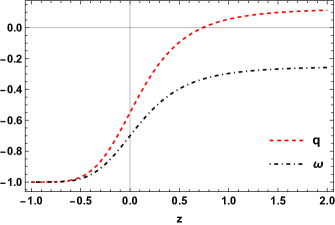
Figure 2: The plot on the left displays density parameters for matter ($\Omega_{m}$), dark energy ($\Omega_{DE}$), and radiation ($\Omega_{r}$) as functions of redshift $z$. The right panel shows the deceleration parameter $q$ and the equation of state parameter $\omega$ as functions of redshift $z$. These two panels illustrate the trajectory for the positive coupling parameter, which can transfer energy from dark matter to dark energy.

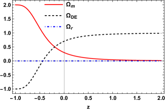
Figure 3: The left panel displays density parameters for matter ($\Omega_{m}$), dark energy ($\Omega_{DE}$), and radiation ($\Omega_{r}$) as functions of redshift $z$. The right panel shows the deceleration parameter $q$ and the equation of state parameter $\omega$ as functions of redshift $z$. These two panels illustrate the trajectory for the negative coupling parameter, which can transfer energy from dark energy to dark matter.

For $n=3/2$ and $\alpha=1/2$ in Fig. 2, $\alpha>0$ indicates that the coupling term $\mathcal{U}>0$, signifying energy transfer from dark matter to dark energy. This figure shows that the universe was dominated by matter in the early stages and will be dominated by dark energy in later stages. Currently, the universe is dominated by dark energy, with parameter values $\Omega_{m}=0.3$, $\Omega_{r}=0.00005$, and $\Omega_{DE}=0.7$, $q_{0}=-0.55$, and $\omega_{0}=-0.70$. For these values, fixed point $P_{1}$ is stable and represents the de Sitter acceleration solution, while fixed point $P_{2}$ is a saddle-node, and $P_{3}$ is an unstable node that cannot demonstrate universal acceleration.
In Fig. 3, with $n=3/2$ and $\alpha=-2$, $\alpha<0$ indicates that the coupling term $\mathcal{U}<0$, that means energy transfers from dark energy to dark matter. This figure shows that the universe was dominated by dark energy in the early stages and will be dominated by dark matter at later stages. Currently, the universe remains dominated by dark energy, with parameter values $\Omega_{m}=0.3$, $\Omega_{r}=0.00005$, and $\Omega_{DE}=0.7$, $q_{0}=-0.563$, and $\omega_{0}=-0.71$. Here, fixed point $P_{3}$ is stable and exhibits acceleration for the early and present universe but fails to show acceleration for late times, while fixed point $P_{1}$ is a saddle-node, and $P_{2}$ is an unstable node. Fig. 4 shows the phase space trajectories of the fixed points $P_{1}$, $P_{2}$, and $P_{3}$.

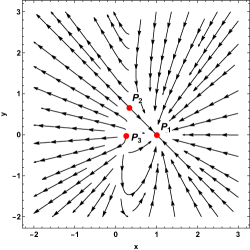
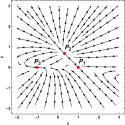
Figure 4: Phase plot of $x$ vs $y$. The upper phase plot shows the stable behavior of $P_{1}$ for $\alpha>0$, and the lower phase plot shows the stable behavior of $P_{3}$ for $\alpha<-1$.

IV.2 For case II

Next, the second case in $f(Q)$ gravity is also investigated in detail for the interacting dark energy system. The models have been systematically constructed with possible ranges of their model parameters derived from the dynamical system analysis within the interacting dark energy framework. It is important to examine how the interaction affects the cosmological viability of the $f(Q)$ gravity models.

The fixed points $(x,y)$ of the dynamical system are the following:

$$R_{1}\mathrel{\mathop{\mathchar 58\relax}}(1,0),\,\,\,\,R_{2}\mathrel{\mathop{\mathchar 58\relax}}\left(\frac{1}{2n},\frac{2n-1}{2n}\right),R_{3}\mathrel{\mathop{\mathchar 58\relax}}\left(\frac{1}{\alpha},\frac{-3\alpha+8n-1}{\alpha}\right),$$

$$R_{4}\mathrel{\mathop{\mathchar 58\relax}}\left(\frac{-\sqrt{-3\alpha+9n^{2}+6\alpha n}-3n}{2\alpha n-\alpha},0\right),$$ (28)

$$R_{5}\mathrel{\mathop{\mathchar 58\relax}}\left(\frac{\sqrt{-3\alpha+9n^{2}+6\alpha n}-3n}{2\alpha n-\alpha},0\right).$$

The corresponding eigenvalues are

$$R_{1}\mathrel{\mathop{\mathchar 58\relax}}\{-4,-3-\alpha\},\,\,\,\,R_{2}\mathrel{\mathop{\mathchar 58\relax}}\{4,1-\frac{\alpha}{2n}\},$$

$$R_{3}\mathrel{\mathop{\mathchar 58\relax}}\{\mathcal{A}_{1}-\frac{4n}{\alpha}+4,-\mathcal{A}_{1}-\frac{4n}{\alpha}+4\},$$

$$R_{4}\mathrel{\mathop{\mathchar 58\relax}}\left\{\frac{5n-1+\mathcal{A}_{2}}{1-2n},\frac{-2\mathcal{A}_{2}^{2}-2(3n-\alpha+2n\alpha)\mathcal{A}_{2}}{(2n-1)^{2}\alpha}\right\},$$

$$R_{5}\mathrel{\mathop{\mathchar 58\relax}}\left\{\frac{-2\mathcal{A}_{2}^{2}+2(3n-\alpha+2n\alpha)\mathcal{A}_{2}}{(2n-1)^{2}\alpha},\frac{1-5n+\mathcal{A}_{2}}{2n-1}\right\}.$$

where $\mathcal{A}_{1}=\frac{2\sqrt{(2n-1)\left(3(\alpha-1)\alpha^{2}+8n^{3}-4n^{2}-6(\alpha-1)\alpha n\right)}}{\alpha-2\alpha n}$ and $\mathcal{A}_{2}=\sqrt{9n^{2}-3\alpha+6n\alpha}$.

IV.2.1 $R_{1}$: the de Sitter fixed point

Corresponding to fixed point $R_{1}\mathrel{\mathop{\mathchar 58\relax}}(x,y)=(1,0)$, the matter density, dark energy density, and effective EoS parameters are

$$\Omega_{m}=0,\,\,\,\,\Omega_{DE}=1,\,\,\,\,\omega=-1.$$ (29)

At this point, both dark matter and radiation are absent, and the universe is dominated by dark energy. The EoS at this fixed point indicates that the universe is experiencing an accelerated expansion. To study the stability of this fixed point, we can analyze the eigenvalues of the Jacobian matrix, which describe the behavior of the fixed point. The eigenvalues for the fixed point $R_{1}$ read

$$\{{-4,\,\,\,-\alpha-3\}}.$$ (30)

The stability behavior of this fixed point is as follows:

• Stable node for $\alpha>-3$,

• Saddle for $\alpha<-3$,

• Non-hyperbolic for $\alpha=-3$.

IV.2.2 $R_{2}$: Non-metricity dominated fixed point

The fixed point $R_{2}$ can be used to explain the late-time accelerating expansion of the universe in $f(Q)$ gravity. The point is given by

$$R_{2}\mathrel{\mathop{\mathchar 58\relax}}(x,y)=\left(\frac{1}{2n},\frac{2n-1}{2n}\right)$$

The characteristics of this critical point solely depend on the model parameter $n$. Corresponding to this fixed point, the matter density, dark energy density, and effective EoS parameters are obtained as

$$\Omega_{m}=0,\,\,\,\,\Omega_{DE}=\frac{1}{2n},\,\,\,\,\omega=-1+\frac{4}{3n}.$$ (31)

The conditions for an accelerating universe are $n<0$ or $n>2$. When $n<0$, the universe exhibits phantom-like behavior, i.e., $\omega<-1$. When $n>2$, the universe exhibits quintessence-like behavior, i.e., $-1<\omega<-1/3$. In this fixed-point solution, we have obtained a matter-dominated era for $n=4/3$ and a radiation-dominated era for $n=1$.
The corresponding eigenvalues for the fixed point $R_{2}$ are as follows:

$$\{{4,\,\,1-\frac{\alpha}{2n}\}}.$$ (32)

We determine the stability of this fixed point for various ranges of $\alpha$. The ranges are as follows:

• Saddle node for $\alpha>2n$,

• Unstable for $\alpha<2n$,

• Non-hyperbolic for $\alpha=2n$.

IV.2.3 $R_{3}$: Scaling solution point

The fixed point $R_{3}$ represents a scaling solution for the universe. This scaling solution makes the ratio $\Omega_{m}/\Omega_{DE}$ constant. The fixed point in this case is given by

$$R_{3}\mathrel{\mathop{\mathchar 58\relax}}(x,y)=\left(\frac{1}{\alpha},\frac{-3\alpha+8n-1}{\alpha}\right).$$

Corresponding to this fixed point, the matter density, dark energy density, and effective EoS parameters read as

$$\Omega_{m}=4-\frac{8n}{\alpha},\,\,\,\,\Omega_{DE}=\frac{1}{\alpha},\,\,\,\,\omega=\frac{8}{3\alpha}-1.$$ (33)

The conditions for an accelerating universe are $\alpha<0$ or $\alpha>4$. When $\alpha<0$, the universe exhibits phantom-like behavior, i.e., $\omega<-1$. When $\alpha>4$, the universe exhibits quintessence-like behavior, i.e., $-1<\omega<-1/3$. In this fixed-point solution, we have obtained a matter-dominated era for $\alpha=8/3$ and a radiation-dominated era for $\alpha=2$. The stability conditions are shown in Fig. 5.

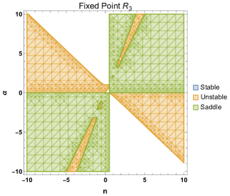
Figure 5: The region plot illustrates the stable, unstable, and saddle behaviors associated with the fixed point $R_{3}$. In this plot, the stable region is very small $\left(\frac{1}{8}<n\leq 0.4393\,\,\text{and}\,\,0<\alpha<\frac{1}{3}(8n-1)\right)$.

IV.2.4 $R_{4}$: Scaling solution point

The fixed point $R_{4}$ represents the scaling solution point of the universe. In addition, it is worth noting that our result modifies the scaling solution with the interacting dark energy parameter $\alpha$. The point $R_{4}$ is

$$R_{4}\mathrel{\mathop{\mathchar 58\relax}}(x,y)=\left(\frac{-\sqrt{-3\alpha+9n^{2}+6\alpha n}-3n}{2\alpha n-\alpha},0\right).$$

Corresponding to this fixed point, the matter density, dark energy density, and effective EoS parameters are obtained as

$$\Omega_{m}=\frac{-\alpha+\sqrt{-3\alpha+9n^{2}+6\alpha n}+(2\alpha+3)n}{\alpha(2n-1)}\,,$$

$$\Omega_{DE}=\frac{-\sqrt{3}\sqrt{-\alpha+3n^{2}+2\alpha n}-3n}{2\alpha n-\alpha}\,,\,\,\text{and}$$

$$w=\frac{-3\alpha-4\alpha n^{2}+2\sqrt{-3\alpha+9n^{2}+6\alpha n}+(8\alpha+6)n}{\alpha(1-2n)^{2}}\,.$$

One can note that all three parameters depend on the model parameter $n$ as well as the interacting parameter $\alpha$. Check appendix A for calculations. The conditions for an accelerating universe and the stability are shown in Figs. 6 and 7.

Figure 6: This plot shows the relationship between the model parameter $n$ and the interacting parameter $\alpha$ for the accelerating universe. The light blue region represents the quintessence-like behavior of an accelerating universe (i.e., $-1<\omega<-1/3$), while the golden region represents the phantom-like behavior of an accelerating universe (i.e., $\omega<-1$).

Figure 7: The region plot illustrates the stable, unstable, and saddle behaviors associated with the fixed point $R_{4}$.

IV.2.5 $R_{5}$: Additional scaling solution point

Corresponding to the fixed point $R_{5}$, that is

$$R_{5}\mathrel{\mathop{\mathchar 58\relax}}(x,y)=\left(\frac{\sqrt{3}\sqrt{-\alpha+3n^{2}+2\alpha n}-3n}{2\alpha n-\alpha},0\right)$$

the matter density, dark energy density, and effective EoS parameters are given by

$$\Omega_{m}=\frac{3n-\sqrt{-3\alpha+9n^{2}+6\alpha n}}{\alpha(2n-1)}+1\,,$$

$$\Omega_{DE}=\frac{\sqrt{-3\alpha+9n^{2}+6\alpha n}-3n}{\alpha(2n-1)}\,,\,\,$$

$$w=\frac{-3\alpha-4\alpha n^{2}-2\sqrt{-3\alpha+9n^{2}+6\alpha n}+(8\alpha+6)n}{\alpha(1-2n)^{2}}\,.$$

The conditions for an accelerating universe and the stability are depicted in Figs. 8 and 9.

Figure 8: The plot show the relationship between the model parameter $n$ and the interacting parameter $\alpha$ for the accelerating universe. The light blue region represents the quintessence-like behavior of an accelerating universe (i.e., $-1<\omega<-1/3$), while the golden region represents the phantom-like behavior of an accelerating universe (i.e., $\omega<-1$).

Figure 9: The region plot illustrates the stable, unstable, and saddle behaviors associated with the fixed point $R_{5}$.

In Figures 10 and 11, we illustrate the evolution of $\Omega_{m}$, $\Omega_{r}$, $\Omega_{DE}$, $q$, and $\omega$ for different values of the model parameter $n$ and the interaction parameter $\alpha$. For $n=3/2$ and $\alpha=4$ in Figure 10, $\alpha>0$ indicates that the coupling term $\mathcal{U}>0$, signifying energy transfer from dark matter to dark energy. This figure shows that the universe was dominated by matter in the early stages and will be dominated by dark energy in later stages. Currently, the universe is dominated by dark energy, with parameter values $\Omega_{m}=0.3$, $\Omega_{r}=0.00005$, and $\Omega_{DE}=0.7$, $q_{0}=-0.548$, and $\omega_{0}=-0.696$. For these values, the fixed points $R_{1}$ and $R_{4}$ are stable and represent the de Sitter and quintessence acceleration solutions, respectively.
In Figure 11, with $n=3/2$ and $\alpha=-4$, $\alpha<0$ indicates that the coupling term $\mathcal{U}<0$, meaning energy transfers from dark energy to dark matter. This figure shows that the universe was dominated by dark energy in the early stages and will be dominated by dark matter in later stages. Currently, the universe remains dominated by dark energy, with parameter values $\Omega_{m}=0.3$, $\Omega_{r}=0.00005$, and $\Omega_{DE}=0.7$, $q_{0}=-0.55$, and $\omega_{0}=-0.70$. For these values, the fixed points $R_{4}$ and $R_{5}$ have imaginary values, and the remaining point cannot exhibit stable behavior.

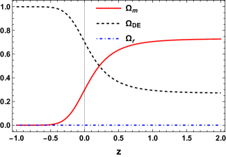
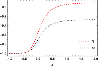
Figure 10: The upper panel displays density parameters for matter ($\Omega_{m}$), dark energy ($\Omega_{DE}$), and radiation ($\Omega_{r}$) as functions of redshift $z$. The lower panel shows the deceleration parameter $q$ and the equation of state parameter $\omega$ as functions of redshift $z$. These two panels illustrate the trajectory for the positive coupling parameter, which can transfer energy from dark matter to dark energy.

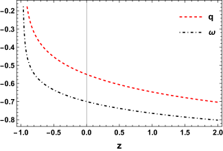
Figure 11: The left panel displays density parameters for matter ($\Omega_{m}$), dark energy ($\Omega_{DE}$), and radiation ($\Omega_{r}$) as functions of redshift $z$. The right panel shows the deceleration parameter $q$ and the equation of state parameter $\omega$ as functions of redshift $z$. These two panels illustrate the trajectory for the negative coupling parameter, which can transfer energy from dark energy to dark matter.

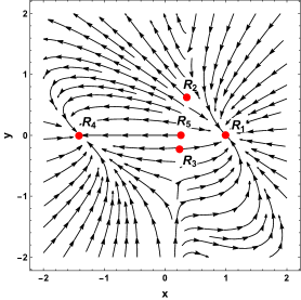
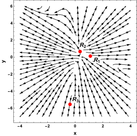
Figure 12: Phase plot of $x$ vs $y$. The phase plot above shows the stable behavior of $R_{1}$ and $R_{4}$ for $\alpha>0$.

V Conclusion

In this work, we have explored the behavior of interacting dark energy and dark matter within $f(Q)$ gravity, employing a standard framework of dynamical system analysis. We have considered the power-law $f(Q)=6\gamma\,H_{0}^{2}\left(\tfrac{Q}{Q_{0}}\right)^{n}$ model incorporating with two different forms of interacting dark energy and dark matter: $3\alpha H\rho_{m}$ and $\frac{\alpha}{3H}\rho_{m}\rho_{DE}$. The parameter $\alpha$ in the interacting terms plays a crucial role in determining the viable conditions and estimating the transition from the matter-dominated era (saddle point) to the dark energy-dominated era (stable node) in viable gravity models at late times. As a result, we have discovered fixed points that can be represented as the late-time accelerating universe in $f(Q)$ gravity. For the form of ${\cal U}=3\alpha H\rho_{m}$, we have illustrated the evolution of $\Omega_{m}$, $\Omega_{r}$, $\Omega_{DE}$, $q$, and $\omega$ for different values of the model parameter $n$ and the interaction parameter $\alpha$. For $n=3/2$ and $\alpha=1/2$ and $\alpha>0$, we found that the coupling term $\mathcal{U}>0$, signifying energy transfer from dark matter to dark energy implying that the universe was dominated by matter in the early stages and would be dominated by dark energy in later stages. With the current data, fixed point $P_{1}$ is stable and represents the de Sitter acceleration solution, while fixed point $P_{2}$ is a saddle node, and $P_{3}$ is an unstable node that cannot demonstrate universal acceleration. Moreover, we have considered another situation of which $n=3/2$ and $\alpha=-2$, $\alpha<0$. We discovered for the coupling term $\mathcal{U}<0$ that energy transfers from dark energy to dark matter. In this case, the universe was dominated by dark energy in the early stages and will be dominated by dark matter in later stages. With the current data, fixed point $P_{3}$ is stable and exhibits acceleration for the early and present universe but fails to show acceleration for late times, while fixed point $P_{1}$ is a saddle node, and $P_{2}$ is an unstable node.

For the form of ${\cal U}=\frac{\alpha}{3H}\rho_{m}\rho_{DE}$, the evolution of $\Omega_{m}$, $\Omega_{r}$, $\Omega_{DE}$, $q$, and $\omega$ for different values of the model parameter $n$ and the interaction parameter $\alpha$ have been examined. We have considered $n=3/2$ and $\alpha=4$ ($\alpha>0$) and found that the coupling term $\mathcal{U}>0$, signifying energy transfer from dark matter to dark energy. Our results show that the universe was dominated by matter in the early stages and would be dominated by dark energy in later stages. Using the observational data, the fixed points $R_{1}$ and $R_{4}$ were stable and would represent the de Sitter and quintessence acceleration solutions. Additionally, for $n=3/2$ and $\alpha=-4$ ($\alpha<0$), we found that the coupling term $\mathcal{U}<0$, meaning energy transfers from dark energy to dark matter implying that the universe was dominated by dark energy in the early stages and would be dominated by dark matter in later stages. Employing the current data, the fixed points $R_{4}$ and $R_{5}$ have imaginary values, and the remaining point cannot exhibit stable behavior.

Although many viable $f(Q)$ models explain the dark energy problem in cosmology, our qualitative results from this work can serve as guidelines for more detailed studies. They can also be used as complementary constraints on viable $f(Q)$ models, alongside other cosmological constraints on $f(Q)$ theories. Our framework, based on the cosmological dynamics of interacting dark energy and dark matter in $f(Q)$ gravity, constitutes the natural template for beyond the standard gravity model, for example, Teleparallel gravity and Gauss-Bonnet gravity, or even more generalizations.

Data Availability Statement

There are no new data associated with this article.

Appendix A Appendix

The conditions of stability for the fixed point $R_{3}$ are as follows:

• For Stable Node:

  $$\frac{1}{8}<n\leq 0.4393\,\,\text{and}\,\,0<\alpha<\frac{1}{3}(8n-1).$$ (34)

• For Unstable Node:

  $$n=0\,\,\text{and}\,\,\left(-\frac{1}{3}<\alpha<0\,\,\text{or}\,\,0<\alpha\leq 1\right),$$ (35)

  $$n<0\,\,\text{and}\,\,\left(\frac{1}{3}(8n-1)<\alpha<2n\right),$$ (36)

  $$0<n\leq\frac{1}{8}\,\,\text{and}\,\,\left(\frac{1}{3}(8n-1)<\alpha<0\right),$$ (37)

  $$n>\frac{1}{2}\,\,\text{and}\,\,2n<\alpha<\frac{1}{3}(8n-1).$$ (38)

• While the saddle point is otherwise.

The conditions of stability for the fixed point $R_{4}$ are as follows:

• For Stable node:

  $$0<n\leq\frac{1}{8}\,\,\text{and}\,\,0<\alpha<-\frac{3n^{2}}{2n-1},$$ (39)

  $$\frac{1}{8}<n<\frac{1}{5}\,\,\text{and}\,\,\frac{1}{3}(8n-1)<\alpha<-\frac{3n^{2}}{2n-1},$$ (40)

  $$\frac{1}{2}<n\leq 1\,\,\text{and}\,\,\alpha>0,$$ (41)

  $$n>1\,\,\text{and}\,\,\left(-\frac{3n^{2}}{2n-1}<\alpha<-3\,\,\text{or}\,\,\alpha>0\right).$$ (42)

• For Unstable node:

  $$n\leq\frac{1}{8}\,\,\text{and}\,\,\alpha<\frac{1}{3}(8n-1),$$ (43)

  $$\frac{1}{8}<n<\frac{1}{2}\,\,\text{and}\,\,\alpha<0.$$ (44)

• While the saddle point is otherwise.

The conditions of stability for the fixed point $R_{5}$ are as follows:

• For Stable node:

  $$n\leq 0\,\,\text{and}\,\,\left(\alpha<-3\,\,\text{or}\,\,0<\alpha<-\frac{3n^{2}}{2n-1}\right),$$ (45)

  $$0<n<\frac{1}{2}\,\,\text{and}\,\,\alpha<-3,$$ (46)

  $$\frac{1}{2}<n<1\,\,\text{and}\,\,-\frac{3n^{2}}{2n-1}<\alpha<-3.$$ (47)

• For Unstable node:

  $$\frac{1}{5}<n<\frac{1}{2}\,\,\text{and}\,\,\frac{1}{3}(8n-1)<\alpha<-\frac{3n^{2}}{2n-1},$$ (48)

  $$n>\frac{1}{2}\,\,\text{and}\,\,\alpha>\frac{1}{3}(8n-1).$$ (49)

• While the saddle point is otherwise.

References

- [1] A. G. Riess et al. [Supernova Search Team], Astron. J. 116, 1009-1038 (1998)
- [2] A. G. Riess, R. P. Kirshner, B. P. Schmidt, S. Jha, P. Challis, P. M. Garnavich, A. A. Esin, C. Carpenter, R. Grashius and R. E. Schild, et al. Astron. J. 117, 707-724 (1999)
- [3] S. Perlmutter et al. [Supernova Cosmology Project], Astrophys. J. 517, 565-586 (1999)
- [4] D. N. Spergel et al. [WMAP], Astrophys. J. Suppl. 148, 175-194 (2003)
- [5] E. Komatsu et al. [WMAP], Astrophys. J. Suppl. 192, 18 (2011)
- [6] D. J. Eisenstein et al. [SDSS], Astrophys. J. 633, 560-574 (2005)
- [7] W. J. Percival et al. [SDSS], Mon. Not. Roy. Astron. Soc. 401, 2148-2168 (2010)
- [8] V. Sahni and A. A. Starobinsky, Int. J. Mod. Phys. D 9, 373 (2000).
- [9] S. M. Carroll, Living Rev. Rel. 4, 1 (2001).
- [10] T. Padmanabhan, Phys. Rept. 380, 235 (2003).
- [11] P. J. E. Peebles and B. Ratra, Rev. Mod. Phys. 75, 559 (2003).
- [12] V. Sahni, Lect. Notes Phys. 653, 141 (2004).
- [13] E. J. Copeland, M. Sami and S. Tsujikawa, Int. J. Mod. Phys. D 15, 1753 (2006).
- [14] S. Nojiri and S. D. Odintsov, eConf C0602061, 06 (2006) [Int. J. Geom. Meth. Mod. Phys. 4, 115 (2007)].
- [15] R. P. Woodard, Lect. Notes Phys. 720, 403 (2007).
- [16] R. Durrer and R. Maartens, Gen. Rel. Grav. 40, 301 (2008).
- [17] F. S. N. Lobo, arXiv:0807.1640 [gr-qc].
- [18] T. P. Sotiriou and V. Faraoni, Rev. Mod. Phys. 82, 451 (2010).
- [19] P. Brax, arXiv:0912.3610 [astro-ph.CO].
- [20] A. De Felice and S. Tsujikawa, Living Rev. Rel. 13, 3 (2010).
- [21] S. Tsujikawa, arXiv:1004.1493 [astro-ph.CO] (Published in ’Dark Matter and Dark Energy: A Challenge for Modern Cosmology’ Series: Astrophysics and Space Science Library, Vol. 370, ISBN: 978-90-481-8684-6, 2011).
- [22] S. Nojiri and S. D. Odintsov, Phys. Rept. 505 (2011), 59-144 [arXiv:1011.0544 [gr-qc]].
- [23] S. Weinberg, Rev. Mod. Phys. 61 (1989), 1-23
- [24] Y. Fujii, Phys. Rev. D 26, 2580 (1982).
- [25] L. H. Ford, Phys. Rev. D 35, 2339 (1987).
- [26] C. Wetterich, Nucl. Phys B. 302, 668 (1988).
- [27] B. Ratra and J. Peebles, Phys. Rev D 37, 321 (1988).
- [28] R. R. Caldwell, R. Dave and P. J. Steinhardt, Phys. Rev. Lett. 80, 1582 (1998).
- [29] G. R. Dvali and M. Zaldarriaga, Phys. Rev. Lett. 88 (2002), 091303
- [30] T. Chiba, T. Okabe and M. Yamaguchi, Phys. Rev. D 62, 023511 (2000).
- [31] C. Armendariz-Picon, V. F. Mukhanov and P. J. Steinhardt, Phys. Rev. Lett. 85, 4438 (2000).
- [32] S. X. Tian and Z. H. Zhu, Phys. Rev. D 103 (2021) no.4, 043518
- [33] S. D. Odintsov, V. K. Oikonomou and F. P. Fronimos, Phys. Dark Univ. 29 (2020), 100563
- [34] S. M. Carroll, Phys. Rev. Lett. 81, 3067 (1998).
- [35] C. F. Kolda and D. H. Lyth, Phys. Lett. B 458, 197 (1999).
- [36] S. Capozziello, Int. J. Mod. Phys. D 11, 483, (2002).
- [37] S. Capozziello, V. F. Cardone, S. Carloni and A. Troisi, Int. J. Mod. Phys. D, 12, 1969 (2003).
- [38] S. M. Carroll, V. Duvvuri, M. Trodden and M. S. Turner, Phys. Rev. D 70, 043528 (2004).
- [39] S. Nojiri and S. D. Odintsov, Phys. Rev. D 68, 123512 (2003).
- [40] L. Amendola, Phys. Rev. D 60, 043501 (1999).
- [41] J. P. Uzan, Phys. Rev. D 59, 123510 (1999).
- [42] T. Chiba, Phys. Rev. D 60, 083508 (1999).
- [43] N. Bartolo and M. Pietroni, Phys. Rev. D 61 023518 (2000).
- [44] F. Perrotta, C. Baccigalupi and S. Matarrese, Phys. Rev. D 61, 023507 (2000).
- [45] A. Riazuelo and J. P. Uzan, Phys. Rev. D 66, 023525 (2002).
- [46] A. Nicolis, R. Rattazzi and E. Trincherini, Phys. Rev. D 79, 064036 (2009).
- [47] S. Nojiri, S. D. Odintsov and M. Sasaki, Phys. Rev. D 71, 123509 (2005).
- [48] S. Nojiri and S. D. Odintsov, Phys. Lett. B 631, 1 (2005).
- [49] J. Wainwright and G. F. R. Ellis, Dynamical Systems in Cosmology, Cambridge University Press (1997).
- [50] A. A. Coley, Dynamical systems and cosmology, Kluwer Academic Publishers (2003).
- [51] S. Bahamonde, C. G. Böhmer, S. Carloni, E. J. Copeland, W. Fang and N. Tamanini, Phys. Rept. 775-777 (2018), 1-122 [arXiv:1712.03107 [gr-qc]].
- [52] L. Amendola, D. Polarski and S. Tsujikawa, Phys. Rev. Lett. 98 (2007), 131302 [arXiv:astro-ph/0603703 [astro-ph]].
- [53] L. Amendola, D. Polarski and S. Tsujikawa, Int. J. Mod. Phys. D 16 (2007), 1555-1561 doi:10.1142/S0218271807010936 [arXiv:astro-ph/0605384 [astro-ph]].
- [54] L. Amendola, R. Gannouji, D. Polarski and S. Tsujikawa, Phys. Rev. D 75, 083504 (2007) [arXiv:gr-qc/0612180 [gr-qc]].
- [55] S. Tsujikawa, Lect. Notes Phys. 800, 99-145 (2010) [arXiv:1101.0191 [gr-qc]].
- [56] L. Amendola and S. Tsujikawa, Phys. Lett. B 660 (2008), 125-132 [arXiv:0705.0396 [astro-ph]].
- [57] S. Tsujikawa, Phys. Rev. D 77 (2008), 023507 [arXiv:0709.1391 [astro-ph]].
- [58] S. D. Odintsov and V. K. Oikonomou, Phys. Rev. D 96 (2017) no.10, 104049
- [59] V. K. Oikonomou, Phys. Rev. D 99 (2019) no.10, 104042
- [60] N. Chatzarakis and V. K. Oikonomou, Annals Phys. 419 (2020), 168216
- [61] V. K. Oikonomou, Int. J. Mod. Phys. D 27 (2018) no.05, 1850059
- [62] S. D. Odintsov and V. K. Oikonomou, Phys. Rev. D 99 (2019) no.10, 104070
- [63] N. J. Poplawski, Phys. Rev. D 74 (2006), 084032 [arXiv:gr-qc/0607124 [gr-qc]].
- [64] N. J. Poplawski, [arXiv:gr-qc/0608031 [gr-qc]].
- [65] J. H. He, B. Wang and E. Abdalla, Phys. Rev. D 84 (2011), 123526 [arXiv:1109.1730 [gr-qc]].
- [66] J. H. He and B. Wang, Int. J. Mod. Phys. A 30 (2015) no.28&29, 1545012
- [67] B. L’Huillier, H. A. Winther, D. F. Mota, C. Park and J. Kim, Mon. Not. Roy. Astron. Soc. 468 (2017) no.3, 3174-3183 [arXiv:1703.07357 [astro-ph.CO]].
- [68] D. Samart, B. Silasan and P. Channuie, Phys. Rev. D 104, no.6, 063517 (2021)
- [69] S. D. Odintsov and V. K. Oikonomou, Phys. Rev. D 98 (2018) no.2, 024013 [arXiv:1806.07295 [gr-qc]].
- [70] A. Halder and M. Pandey, [arXiv:2101.05228 [astro-ph.CO]].
- [71] J. Beltrán Jiménez, D. Rubiera-Garcia, D. Sáez-Gómez and V. Salzano, Phys. Rev. D 94 (2016) no.12, 123520
- [72] J. B. Jimenez et al., Phys. Rev. D 98, 044048 (2018).
- [73] J. B. Jimenez et al., Phys. Rev. D 101, 103507 (2020).
- [74] N. Frusciante, Phys. Rev. D 103, 044021 (2021).
- [75] K. F. Dialektopoulos, T. S. Koivisto and S. Capozziello, Eur. Phys. J. C 79(7), 606 (2019).
- [76] K. Flathmann and M. Hohmann, Phys. Rev. D 103, 044030 (2021).
- [77] I. Ayuso, R. Lazkoz and V. Salzano, Phys. Rev. D 103, 063505 (2021).
- [78] B. J. Barros, T. Barreiro, T. Koivisto and N. J. Nunes, Phys. Dark Univ. 30, 100616 (2020).
- [79] F. Bajardi, D. Vernieri and S. Capozziello, Eur. Phys. J. Plus 135, 912 (2020).
- [80] I. Soudi et al., Phys. Rev. D 100, 044008 (2019).
- [81] J.B. Jimenez, L. Heisenberg, and T. S. Koivisto, Universe 5, 173 (2019).
- [82] T. Harko et al., Phys. Rev. D 98, 084043 (2018).
- [83] Y. Xu, G. Li, T. Harko, and S.D. Liang, Eur. Phys. J. C 79, 708 (2019).
- [84] L. Jarv, M. Runkla, M. Saal, and O. Vilson, Phys. Rev. D 97, 124025 (2018).
- [85] R. Lazkoz et al., Phys. Rev. D 100, 104027 (2019).
- [86] I. Ayuso, R. Lazkoz, and V. Salzano, Phys. Rev. D 103, 063505 (2021).
- [87] W. Khyllep, A. Paliathanasis and J. Dutta, Phys. Rev. D 103, 103521 (2021).
- [88] Bruno J. Barros et al., Phys. Dark Univ. 30, 100616 (2020).
- [89] F. K. Anagnostopoulos, S. Basilakos, and E. N. Saridakis, Phys. Lett. B 822, 136634 (2021).
- [90] S. Mandal, P. K. Sahoo, Phys. Lett. B 823, 136786 (2021).
- [91] L. Atayde, N. Frusciante, Phys. Rev. D 104, 064052 (2021).
- [92] I. Soudi et al., Phys. Rev. D 100, 9044008 (2019).
- [93] Ruth Lazkoz et al., Phys. Rev. D 100, 104027 (2019).
- [94] I. Ayuso, R. Lazkoz, and V. Salzano, Phys. Rev. D 103, 063505 (2021).
- [95] N. Frusciante, Phys. Rev. D 103, 044021 (2021).
- [96] F. A. Anagnostopoulos et al., Eur. Phys. J. C 83, 58 (2023).
- [97] O. Sokoliuk et al., Mon. Not. Roy. Astron. Soc. 522, 252–267 (2023).
- [98] Gaurav N Gadbail, S. Mandal, P.K. Sahoo, Phys. Lett. B, 835, 137509 (2022).
- [99] Jianbo Lua, Xin Zhao, and Guoying Chee, Eur. Phys. J. C 79, 530 (2019).
- [100] W. Khyllep et al., Phys. Rev. D 107, 044022 (2023).
- [101] A. Paliathanasis, Phys. Dark Univ. 41, 101255 (2023).
- [102] S.A. Narawade, S. P. Singh, and B. Mishra, Phys. Dark Univ. 42, 101282 (2023).
- [103] C. Bohmer, E. Jensko 1 and R. Lazkoz, Universe 9, 166 (2023).
- [104] S. Ghosh, R. Solanki, and P.K. Sahoo, Phys. Scr. 99, 055021 (2024).