Verifying the Generalization of Deep Learning to Out-of-Distribution Domains

Abstract

Deep neural networks (DNNs) play a crucial role in the field of machine learning, demonstrating state-of-the-art performance across various application domains. However, despite their success, DNN-based models may occasionally exhibit challenges with generalization, i.e., may fail to handle inputs that were not encountered during training. This limitation is a significant challenge when it comes to deploying deep learning for safety-critical tasks, as well as in real-world settings characterized by substantial variability. We introduce a novel approach for harnessing DNN verification technology to identify DNN-driven decision rules that exhibit robust generalization to previously unencountered input domains. Our method assesses generalization within an input domain by measuring the level of agreement between independently trained deep neural networks for inputs in this domain. We also efficiently realize our approach by using off-the-shelf DNN verification engines, and extensively evaluate it on both supervised and unsupervised DNN benchmarks, including a deep reinforcement learning (DRL) system for Internet congestion control — demonstrating the applicability of our approach for real-world settings. Moreover, our research introduces a fresh objective for formal verification, offering the prospect of mitigating the challenges linked to deploying DNN-driven systems in real-world scenarios.

1 Introduction

In the last decade, deep learning [1] has demonstrated state-of-the-art performance in natural language processing, image recognition, game playing, computational biology, and numerous other fields [2, 3, 4, 5, 6, 7, 8]. Despite its remarkable success, deep learning still faces significant challenges that restrict its applicability in domains involving safety-critical tasks or inputs with high variability.

One critical limitation lies in the well-known challenge faced by deep neural networks (DNNs) when attempting to generalize to novel input domains. This refers to their tendency to exhibit suboptimal performance on inputs significantly different from those encountered during training. Throughout the training process, a DNN is exposed to input data sampled from a specific distribution over a designated input domain (referred to as “in-distribution” inputs). The rules derived from this training may falter in generalizing to novel, unencountered inputs, due to several factors: (1) the DNN being invoked in an out-of-distribution (OOD) scenario, where there is a mismatch between the distribution of inputs in the training data and that in the DNN’s operational data; (2) certain inputs not being adequately represented in the finite training dataset (such as various, low-probability corner cases); and (3) potential “overfitting” of the decision rule to the specific training data.

The importance of establishing the generalizability of (unsupervised) DNN-based decisions is evident in recently proposed applications of deep reinforcement learning (DRL) [9]. Within the framework of DRL, an agent, implemented as a DNN, undergoes training through repeated interactions with its environment to acquire a decision-making policy achieving high performance concerning a specific objective (“reward”). DRL has recently been applied to numerous real-world tasks [10, 11, 12, 13, 14, 15, 16, 17, 18, 19]. In many DRL application domains, the learned policy is anticipated to perform effectively across a broad spectrum of operational environments, with a diversity that cannot possibly be captured by finite training data. Furthermore, the consequences of inaccurate decisions can be severe. This point is exemplified in our examination of DRL-based Internet congestion control (discussed in Sec. 4.3). Good generalization is also crucial for non-DRL tasks, as we shall illustrate through the supervised-learning example of Arithmetic DNNs.

We introduce a methodology designed to identify DNN-based decision rules that exhibit strong generalization across a range of distributions within a specified input domain. Our approach is rooted in the following key observation. The training of a DNN-based model encompasses various stochastic elements, such as the initialization of the DNN’s weights and the order in which inputs are encountered during training. As a result, even when DNNs with the same architecture undergo training to perform an identical task on the same training data, the learned decision rules will typically exhibit variations. Drawing inspiration from Tolstoy’s Anna Karenina [20], we argue that “successful decision rules are all alike; but every unsuccessful decision rule is unsuccessful in its own way”. To put it differently, we believe that when scrutinizing decisions made by multiple, independently trained DNNs on a specific input, consensus is more likely to occur when their (similar) decisions are accurate.

Given the above, we suggest the following heuristic for crafting DNN-based decision rules with robust generalization across an entire designated input domain: independently train multiple DNNs and identify a subset that exhibits strong consensus across all potential inputs within the specified input domain. This implies, according to our hypothesis, that the learned decision rules of these DNNs generalize effectively to all probability distributions over this domain. Our evaluation, as detailed in Sec. 4, underscores the tremendous effectiveness of this methodology in distilling a subset of decision rules that truly excel in generalization across inputs within this domain. As our heuristic aims to identify DNNs whose decisions unanimously align for every input in a specified domain, the decision rules derived through this approach consistently achieve high levels of generalization, across all benchmarks.

Since our methodology entails comparing the outputs of various DNNs across potentially infinite input domains, the utilization of formal verification is a natural choice. In this regard, we leverage recent advancements in the formal verification of DNNs [21, 22, 23, 24, 25, 26, 27, 28, 29]. Given a verification query comprised of a DNN $N$, a precondition $P$, and a postcondition $Q$, a DNN verifier is tasked with determining whether there exists an input $x$ to $N$ such that $P(x)$ and $Q(N(x))$ both hold. To date, DNN verification research has primarily concentrated on establishing the local adversarial robustness of DNNs, i.e., identifying small input perturbations that lead to the DNN misclassifying an input of interest [30, 31, 32]. Our approach extends the scope of DNN verification by showcasing, for the first time (as far as we are aware), its utility in identifying DNN-based decision rules that exhibit robust generalization. Specifically, we demonstrate how, within a defined input domain, a DNN verifier can be employed to assign a score to a DNN that indicates its degree of agreement with other DNNs throughout the input domain in question. This, in turn, allows an iterative process for the gradual pruning of the candidate DNN set, retaining only those that exhibit strong agreement and are likely to generalize successfully.

To assess the effectiveness of our methodology, we concentrate on three widely recognized benchmarks in the field of deep reinforcement learning (DRL): (i) Cartpole, where a DRL agent learns to control a cart while balancing a pendulum; (ii) Mountain Car, which requires controlling a car to escape from a valley; and (iii) Aurora, designed as an Internet congestion controller. Aurora stands out as a compelling case for our approach. While Aurora is designed to manage network congestion in a diverse range of real-world Internet environments, its training relies solely on synthetically generated data. Therefore, for the deployment of Aurora in real-world scenarios, it is crucial to ensure the soundness of its policy across numerous situations not explicitly covered by its training inputs.

Additionally, we consider a benchmark from the realm of supervised learning, namely, DNN-based arithmetic learning, in which the goal is to train a DNN to correctly perform arithmetic operations. Arithmetic DNNs are a natural use-case for demonstrating the applicability of our approach to a supervised learning (and so, non-DRL) setting, and since generalization to OOD domains is a primary focus in this context and is perceived to be especially challenging [33, 34]. We demonstrate how our approach can be employed to assess the capability of Arithmetic DNNs to execute learned operations on ranges of real numbers not encountered in training.

The results of our evaluation indicate that, across all benchmarks, our verification-driven approach effectively ranks DNN-based decision rules based on their capacity to generalize successfully to inputs beyond their training distribution. In addition, we present compelling evidence that our formal verification method is superior to competing methods, namely gradient-based optimization methods and predictive uncertainty methods. These findings highlight the efficacy of our approach. Our code and benchmarks are publicly available as an artifact accompanying this work [35].

The rest of the paper is organized in the following manner. Sec. 2 provides background on DNNs and their verification procedure. In Sec. 3 we present our verification-driven approach for identifying DNN-driven decision rules that generalize successfully to OOD input domains. Our evaluation is presented in Sec. 4, and a comparison to competing optimization methods is presented in Sec. 5. Related work is covered in Sec. 6, limitations are covered in Sec. 7, and our conclusions are provided in Sec. 8. We include appendices with additional information regarding our evaluation.

Note. This is an extended version of our paper, titled “Verifying Generalization in Deep Learning” [36], which appeared at the Computer Aided Verification (CAV) 2023 conference. In the original paper, we presented a brief description of our method, and evaluated it on two DRL benchmarks, while giving a high-level description of its applicability to additional benchmarks. In this extended version, we significantly enhance our original paper along multiple axes, as explained next. In terms of our approach, we elaborate on how to strategically design a DNN verification query for the purpose of executing our methods, and we also elaborate on various distance functions leveraged in this context. We also incorporate a section on competing optimization methods, and showcase the advantages of our approach compared to gradient-based optimization techniques. We significantly enhance our evaluation in the following manner: (i) we demonstrate the applicability of our approach to supervised learning, and specifically to Arithmetic DNNs (in fact, to the best of our knowledge, we are the first to verify Arithmetic DNNs); and (ii) we enhance the previously presented DRL case study to include additional results and benchmarks. We believe these additions merit an extended paper, which complements our original, shorter one [36].

2 Background

Deep Neural Networks (DNNs) [1] are directed graphs comprising several layers, that subsequently compute various mathematical operations. Upon receiving an input, i.e., assignment values to the nodes of the DNN’s first (input) layer, the DNN propagates these values, layer after layer, until eventually reaching the final (output) layer, which computes the assignment of the received input. Each node computes the value based on the type of operations to which it is associated. For example, nodes in weighted-sum layers, compute affine combinations of the values of the nodes in the preceding layer to which they are connected. Another popular layer type is the rectified linear unit (ReLU) layer, in which each node $y$ computes the value $y=\text{ReLU}{}(x)=\max(x,0)$, in which $x$ is the output value of a single node from the preceding layer. For more details on DNNs and their training procedure, see [1]. Fig. 1 depicts an example of a toy DNN. Given input $V_{1}=[2,1]^{T}$, the second layer of this toy DNN computes the (weighted sum) $V_{2}=[7,-6]^{T}$. Subsequently, the ReLU functions are applied in the third layer, resulting in $V_{3}=[7,0]^{T}$. Finally, the DNN’s single output is accordingly calculated as $V_{4}=[14]$.

Figure 1: A toy DNN.

Deep Reinforcement Learning (DRL) [9] is a popular paradigm in machine learning, in which a reinforcement learning (RL) agent, realized as a DNN, interacts with an environment across multiple time-steps $t\in\{0,1,2,\ldots\}$. At each discrete time-step, the DRL agent observes the environment’s state $s_{t}\in\mathcal{S}$, and selects an action $N(s_{t})=a_{t}\in\mathcal{A}$ accordingly. As a result of this action, the environment may change and transition to its next state $s_{t+1}$, and so on. During training, at each time-step, the environment also presents the agent with a reward $r_{t}$ based on its previously chosen action. The agent is trained by repeatedly interacting with the environment, with the goal of maximizing its expected cumulative discounted reward $R_{t}=\mathbb{E}\big{[}\sum_{t}\gamma^{t}\cdot r_{t}\big{]}$, where $\gamma\in\big{[}0,1\big{]}$ is a discount factor, i.e., a hyperparameter that controls the accumulative effect of past decisions on the reward. For additional details, see [37, 38, 39, 40, 41, 42].

Supervised Learning (SL) is another popular machine learning (ML) paradigm. In SL, the input is a dataset of training data comprising pairs of inputs and their ground-truth labels $(x_{i},y_{i})$, drawn from some (possibly unknown) distribution $\mathcal{D}$. The dataset is used to train a model to predict the correct output label for new inputs drawn from the same distribution.

Arithmetic DNNs. Despite the success of DNNs in many SL tasks, they (surprisingly) fail to generalize for the simple SL task of attempting to learn arithmetic operations [33]. When trained to perform such tasks, they often succeed for inputs sampled from the distribution on which they were trained, but their performance significantly deteriorates when tested on inputs drawn OOD, e.g., input values from another domain. This behavior is indicative of Arithmetic DNNs tending to overfit their training data rather than systematically learning from it. This is observed even in the context of simple arithmetic tasks, such as approximating the identity function, or learning to sum up inputs. A common belief is that the limitations of the classic learning processes, combined with DNNs’ over-parameterized nature, prevent them from learning to generalize arithmetic operations successfully [33, 34].

DNN Verification. A DNN verifier [43] receives the following inputs: (i) a (trained) DNN $N$; (ii) a precondition $P$ on the inputs of the DNN, effectively limiting the possible assignments to be part of a domain of interest; and (iii) a postcondition $Q$ on the outputs of the DNN. A sound DNN verifier can then respond in one of the following two ways: (i) SAT, along with a concrete input $x^{\prime}$ for which the query $P(x^{\prime})\wedge Q(N(x^{\prime}))$ is satisfied; or (ii) UNSAT, indicating no such input $x^{\prime}$ exists. Typically, the postcondition $Q$ encodes the negation of the DNN’s desirable behavior for all inputs satisfying $P$. Hence, a SAT result indicates that the DNN may err, and that $x^{\prime}$ is an example of an input in our domain of interest, that triggers a bug; whereas an UNSAT result indicates that the DNN always performs correctly.

For example, let us revisit the DNN in Fig. 1. Suppose that we wish to verify that for all non-negative inputs the toy DNN outputs a value strictly smaller than $25$, i.e., for all inputs $x=\langle v_{1}^{1},v_{1}^{2}\rangle\in\mathbb{R}^{2}_{\geq 0}$, it holds that $N(x)=v_{4}^{1}<25$. This is encoded as a verification query by choosing a precondition restricting the inputs to be non-negative, i.e., $P=(v^{1}_{1}\geq 0\wedge v_{1}^{2}\geq 0)$, and by setting $Q=(v_{4}^{1}\geq 25)$, which is the negation of our desired property. For this specific verification query, a sound verifier will return SAT, alongside a feasible counterexample such as $x=\langle 1,3\rangle$, which produces $v_{4}^{1}=26\geq 25$. Hence, this property does not hold for the DNN described in Fig. 1. To date, a plethora of DNN verification engines have been put forth [44, 43, 30, 45, 31, 46], mostly used in the context of validating the robustness of a general DNN to local adversarial perturbations.

3 Quantifying Generalizability via Verification

Our strategy for evaluating a DNN’s potential for generalization on out-of-distribution inputs is rooted in the “Karenina hypothesis”: while there might be numerous (potentially infinite) ways to generate incorrect results, correct outputs are likely to be quite similar . Therefore, to pinpoint DNN-based decision rules that excel at generalizing to new input domains, we propose the training of multiple DNNs and assessing the learned decision models based on the alignment of their outputs with those of other models in the domain. As we elaborate next, this scoring procedure can be conducted using a backend DNN verifier. We show how to effectively distill DNNs that successfully generalize OOD, by iteratively filtering out models that tend to disagree with their peers.

3.1 Our Iterative Procedure

To facilitate our reasoning about the agreement between two DNN-based decision rules over an input domain, we introduce the following definitions.

Intuitively, a distance function allows to quantify the (dis)agreement level between the decisions of two DNNs, when fed the same input. We elaborate later on examples of various distance functions that were used.

This definition captures the notion that for every possible input in our domain $\Psi$, DNNs $N_{1}$ and $N_{2}$ produce outputs that are (at most) $\alpha$-distance apart from each other. Small $\alpha$ values indicate that the $N_{1}$ and $N_{2}$ produce “close” values for all inputs in the domain $\Psi$, whereas a large $\alpha$ values indicate that there exists an input in $\Psi$ for which there is a notable divergence between both decision models.

To calculate PDT values, our method utilizes verification to perform a binary search aiming to find the maximum distance between the outputs of a pair of DNNs; see Alg. 1.

Algorithm 1 Pairwise Disagreement Threshold

Input: DNNs ($N_{i}$, $N_{j}$), input domain $\Psi$, distance function $d$, max. disagreement $\texttt{M}>0$
Output: $\text{PDT}(N_{i},N_{j})$

1:$\texttt{low}\leftarrow 0$, $\texttt{high}\leftarrow\texttt{M}$

2:while $\left(\texttt{low}<\texttt{high}\right)$ do

3:     $\alpha\leftarrow\frac{1}{2}\cdot(\texttt{low}+\texttt{high})$

4:     query $\leftarrow$ SMT SOLVER $\langle P\leftarrow\Psi,[N_{i};N_{j}],Q\leftarrow d(N_{i},N_{j})\geq\alpha\rangle$

5:     if query is SAT then: $\texttt{low}\leftarrow\alpha$

6:     else if query is UNSAT then: $\texttt{high}\leftarrow\alpha$

7:end while

8:return $\alpha$

After being calculated, the Pairwise disagreement thresholds can subsequently be aggregated to measure the overall disagreement between a decision model and a set of other decision models, as defined next.

Intuitively, a disagreement score of a single DNN decision model measures the degree to which it tends to disagree, on average, with the remaining models.

Iterative Scheme. Leveraging disagreement scores, our heuristic employs an iterative process (see Alg. 2) to choose a subset of models that exhibit generalization to out-of-distribution scenarios — as encoded by inputs in $\Psi$. At first, $k$ DNNs $\{N_{1},N_{2},\ldots,N_{k}\}$ are trained independently on the training data. Next, a backend verifier is invoked in order to calculate, per each of the ${k\choose 2}$ DNN pairs, their respective pairwise-disagreement threshold (up to some accuracy, $\epsilon$). Next, our algorithm iteratively: (i) calculates the disagreement score of each model in the remaining model subset; (ii) identifies models with (relatively) high $DS$ scores; and (iii) removes them from the model set (Line 9 in Alg. 2). We also note that the algorithm is given an upper bound (M) on the maximum difference, as informed by the user’s domain-specific knowledge.

Termination. The procedure terminates after it exceeds a predefined number of iterations (Line 3 in Alg. 2), or alternatively, when all remaining models “agree” across the input domain $\Psi$, as indicated by nearly identical disagreement scores (Line 7 in Alg. 2).

Algorithm 2 Model Selection Procedure

Input: Set of models $\mathcal{N}=\{N_{1},\ldots,N_{k}\}$, max disagreement M, number of ITERATIONS
Output: $\mathcal{N^{\prime}}\subseteq\mathcal{N}$

1:PDT $\leftarrow$ Pairwise Disagreement Thresholds($\mathcal{N},d,\Psi,\texttt{M}$) $\triangleright$ table with all PDTs

2:$\mathcal{N^{\prime}}\leftarrow\mathcal{N}$

3:for $l=1\ldots$ITERATIONS  do

4:     for $N_{i}\in\mathcal{N^{\prime}}$ do

5:         currentDS[$N_{i}$] $\leftarrow DS_{\mathcal{N^{\prime}}}(N_{i},\texttt{PDT})$ $\triangleright$ based on Definition 3.3

6:     end for

7:     if modelScoresAreSimilar(currentDS) then: break

8:     $\texttt{modelsToRemove}\leftarrow\texttt{findModelsWithHighestDS({currentDS})}$

9:     $\mathcal{N^{\prime}}\leftarrow\mathcal{N^{\prime}}\setminus\texttt{modelsToRemove}$ $\triangleright$ remove models that may disagree

10:end for

11:return $\mathcal{N^{\prime}}$

DS Removal Threshold. There are various possible criteria for determining the DS threshold above for which models are removed, as well as the number of models to remove in each iteration (Line 8 in Alg. 2). In our evaluation, we used a simple and natural approach, of iteratively removing the $p\%$ models with the highest disagreement scores, for some choice of $p$ ($p=25\%$ in our case). A thorough discussion of additional filtering criteria (all of which proved successful, on all benchmarks) is relegated to Appendix D.

3.2 Verification Queries

Next, we elaborate on how we encoded the queries, which we later fed to our backend verification engine (Line 4 in Alg. 1), in order to compute the PDT scores for a DNN pair.

Given a DNN pair, $N_{1}$ and $N_{2}$, we execute the following stages:

1. Concatenate $N_{1}$ and $N_{2}$ to a new DNN $N_{3}=[N_{1};N_{2}]$, which is roughly twice the size of each of the original DNNs (as both $N_{1}$ and $N_{2}$ have the same architecture). The input of $N_{3}$ is of the same original size as each single DNN and is connected to the second layer of each DNN, consequently allowing the same input to flow throughout the network to the output layers of $N_{1}$ and $N_{2}$. Thus, the output layer of $N_{3}$ is a concatenation of the outputs of both $N_{1}$ and $N_{2}$. A scheme depicting the construction of a concatenated DNN appears in Fig. 2.

2. Encode a precondition P which represents the ranges of value assignments to the input variables. As we mentioned before, the value-range bounds are supplied by the system designer, based on prior knowledge of the input domain. In some cases, these values can be predefined to match a specific OOD setting evaluated. In others, these values can be extracted based on empirical simulations of the models post-training. For additional details, we refer the reader to Appendix C.

3. Encode a postcondition Q which encapsulates (for a fixed slack $\alpha$) and a given distance function $d:\mathcal{O}\times\mathcal{O}\mapsto\mathbb{R^{+}}$, that for an input $x^{\prime}\in\Psi$ the following holds:

   $$d(N_{1}(x^{\prime}),N_{2}(x^{\prime}))\geq\alpha$$

   Examples of distance functions include:

   1. $L_{1}$ norm:

      $$d(N_{1},N_{2})=\operatorname*{arg\,max}_{x\in\Psi}(|N_{1}(x)-N_{2}(x)|)$$

      This distance function is used in our evaluation of the Aurora and Arithmetic DNNs benchmarks.

   2. $\mathbf{\textbf{condition-distance}(``\text{c-distance}^{\prime\prime})}$:

      This function returns the maximal $L_{1}$ norm of two DNNs, for all inputs $x\in\Psi$ such that both outputs $N_{1}(x)$, $N_{2}(x)$ comply to constraint $\mathbf{c}$.

      $$\text{c-distance}(N_{1},N_{2})\triangleq\max_{x\in\Psi\text{ s.t. }N_{1}(x),N_{2}(x)\vDash c}(|N_{1}(x)-N_{2}(x)|)$$

      This distance function is used in our evaluation of the Cartpole and Mountain Car benchmarks. In these cases, we defined the distance function to be:

      $$d(N_{1},N_{2})=\min_{c,c^{\prime}}(\text{c-distance}(N_{1},N_{2}),\text{c'-distance}(N_{1},N_{2}))$$

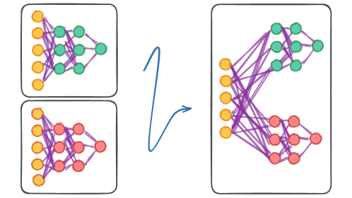
Figure 2: To calculate the PDT scores, we generated a new DNN that is the concatenation of each pair of DNNs (sharing the same input).

4 Evaluation

Benchmarks. We extensively evaluated our method using four benchmarks: (i) Cartpole; (ii) Mountain Car; (iii) Aurora; and (iv) Arithmetic DNNs. The first three are DRL benchmarks, whereas the fourth is a challenging supervised learning benchmark. Our evaluation of DRL systems spans two classic DRL settings, Cartpole [47] and Mountain Car [48], as well as the recently proposed Aurora congestion controller for Internet traffic [14]. We also extensively evaluate our approach on Arithmetic DNNs, i.e., DNNs trained to approximate mathematical operations (such as addition, multiplication, etc.).

Setup. For each of the four benchmarks, we initially trained multiple DNNs with identical architectures, varying only the random seed employed in the training process. Subsequently, we removed from this set all the DNNs but the ones that achieved high reward values (in the DRL benchmarks) or high precision (in the supervised-learning benchmark) in-distribution, in order to rule out the chance that a decision model exhibits poor generalization solely because of inadequate training. Next, we specified out-of-distribution input domains of interest for each specific benchmark and employed Alg. 2 to choose the models deemed most likely to exhibit good generalization on those domains according to our framework. To determine the ground truth regarding the actual generalization performance of different models in practice, we applied the models to inputs drawn from the considered OOD domain, and ranked them based on empirical performance (average reward/maximal error, depending on the benchmark). To assess the robustness of our results, we performed the last step with different choices of probability distributions over the inputs in the domain.

Verification. All queries were dispatched using Marabou [49, 50] — a sound and complete DNN verification engine, which is capable of addressing queries regarding a DNN’s characteristics by converting them into SMT-based constraint satisfaction problems. The Cartpole benchmark included $48,000$ queries ($24,000$ queries per each of the two platform sides), all of which terminated within $12$ hours. The Mountain Car benchmark included $10,080$ queries, all of which terminated within one hour. The Aurora benchmark included $24,000$ verification queries, out of which all but $12$ queries terminated within $12$ hours; and the remaining ones hit the time-out threshold. Finally, the Arithmetic DNNs benchmark included $2,295$ queries, running with a time-out value of $24$ hours; all queries terminated, with over $96\%$ running in less than an hour, and the longest non-DRL query taking slightly less than $13.8$ hours. All benchmarks ran on a single CPU, and with a memory limit of either $1$ GB (for Arithmetic DNNs) or $2$ GB (for the DRL benchmarks). We note that in the case of the Arithmetic DNNs benchmark — Marabou internally used the Guorobi LP solver as a backend engine when dealing with these queries.

Results. The findings support our claim that models chosen using our approach are expected to significantly outperform other models for inputs drawn from the OOD domain considered. This is the case for all evaluated settings and benchmarks, regardless of the chosen hyperparameters and filtering criteria. We note that although our approach can potentially also remove some of the successful models, in all benchmarks, and across all evaluations, it managed to remove all unsuccessful models. Next, we provide an overview of our evaluation. A comprehensive exposition and additional details can be found in the appendices. Our code and benchmarks are publicly available online [35].

4.1 Cartpole

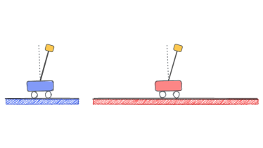
Figure 3: Cartpole: in-distribution setting (blue) and OOD setting (red).

Cartpole [51] is a widely known RL benchmark where an agent controls the motion of a cart with an inverted pendulum (“pole”) affixed to its top. The cart traverses a platform, and the objective of the agent is to maintain balance for the pole for as long as possible (see Fig. 3).

Agent and Environment. The agent is provided with inputs, denoted as $s=(x,v_{x},\theta,v_{\theta})$, where $x$ represents the cart’s position on the platform, $\theta$ represents the angle of the pole (with $|\theta|$ approximately $0$ for a balanced pole and $|\theta|$ approximately $90\degree$ for an unbalanced pole), $v_{x}$ indicates the cart’s horizontal velocity, and $v_{\theta}$ denotes the pole’s angular velocity.

In-Distribution Inputs. During the training process, the agent is encouraged to balance the pole while remaining within the boundaries of the platform. In each iteration, the agent produces a single output representing the cart’s acceleration (both sign and magnitude) for the subsequent step. Throughout the training, we defined the platform’s limits as $[-2.4,2.4]$, and the initial position of the cart as nearly static and close to the center of the platform (as depicted on the left-hand side of Fig. 3). This was accomplished by uniformly sampling the initial state vector values of the cart from the range $[-0.05,0.05]$.

(OOD) Input Domain. We examine an input domain with larger platforms compared to those utilized during training. Specifically, we extend the range of the $x$ coordinate in the input vectors to cover [-10, 10]. The bounds for the other inputs remain the same as during training. For additional details, see Appendices A and C.

Evaluation. We trained a total of $k=16$ models, all of which demonstrated high rewards during training on the short platform. Subsequently, we applied Alg. 2 until convergence (requiring $7$ iterations in our experiments) on the aforementioned input domain. This resulted in a collection of 3 models. We then subjected all $16$ original models to inputs that were drawn from the new, OOD domain. The generated distribution was crafted to represent a novel scenario: the cart is now positioned at the center of a considerably longer, shifted platform (see the red-colored cart depicted in Fig. 3).

All remaining parameters in the OOD environment matched those used for the original training. Figure 4 presents the outcomes of evaluating the models on $20,000$ OOD instances. Out of the initial $16$ models, $11$ achieved low to mediocre average rewards, demonstrating their limited capacity to generalize to this new distribution. Only $5$ models attained high reward values on the OOD domain, including the $3$ models identified by our approach; thus indicating that our method successfully eliminated all $11$ models that would have otherwise exhibited poor performance in this OOD setting (see Fig. 5). For more information, we refer the reader to Appendix E.

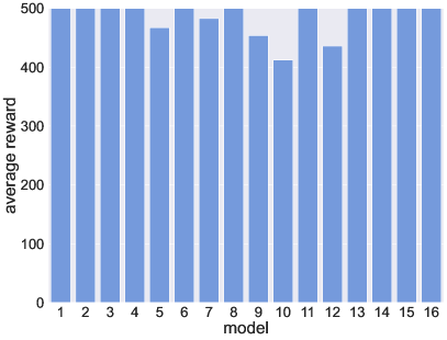
(a)

(b)

Figure 4: Cartpole: models’ average rewards in different distributions.

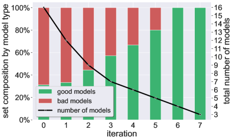
Figure 5: Cartpole: Alg. 2’s results, per iteration: the bars represent the ratio of good and bad models in the surviving set (left y-axis), while the curve indicates the number of surviving models (right y-axis). Our technique selected models {6,7,9}.

4.2 Mountain Car

For our second experiment, we evaluated our method on the Mountain Car [52] benchmark, in which an agent controls a car that needs to learn how to escape a valley and reach a target (see Fig. 6).

Agent and Environment. The car (agent) is placed in a valley between two hills (at $x\in[-1.2,0.6]$), and needs to reach a flag on top of one of the hills. The state, $s=(x,v_{x})$ represents the car’s location (along the x-axis) and velocity. The agent’s action (output) is the applied force: a continuous value indicating the magnitude and direction in which the agent wishes to move. During training, the agent is incentivized to reach the flag (placed at the top of a valley, originally at $x=0.45$). For each time-step until the flag is reached, the agent receives a small, negative reward; if it reaches the flag, the agent is rewarded with a large positive reward. An episode terminates when the flag is reached, or when the number of steps exceeds some predefined value ($300$ in our experiments). Good and bad models are distinguished by an average reward threshold of 90.

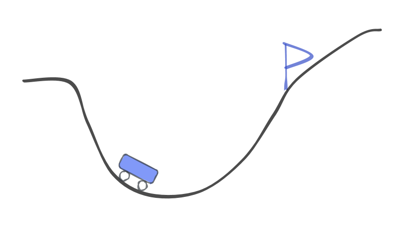
(a) Training (in-distribution) setting: the agent’s initial point is on the left side, and the goal is at a nearby point

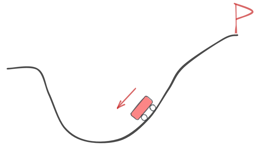
(b) OOD setting: the agent’s initial point is farther away, with initial negative velocity; the goal is significantly farther up than during training

Figure 6: Mountain Car: figure (a) depicts the setting in which the agents were trained, and figure (b) depicts the harder, OOD setting.

In-Distribution Inputs. During training (in-distribution), the car is initially placed on the left side of the valley’s bottom, with a low, random velocity (see Fig. 6(a)). We trained $k=16$ agents (denoted as $\{1,2,\ldots 16\}$), which all perform well, i.e., achieve an average reward higher than our threshold, in-distribution. This evaluation was conducted over $10,000$ episodes.

(OOD) Input Domain. According to the scenarios used by the training environment, we specified the (OOD) input domain by: (i) extending the x-axis, from $[-1.2,0.6]$ to $[-2.4,0.9]$; (ii) moving the flag further to the right, from $x=0.45$ to $x=0.9$; and (iii) setting the car’s initial location further to the right of the valley’s bottom, and with a large initial negative velocity (to the left). An illustration appears in Fig. 6(b). These new settings represent a novel state distribution, which causes the agents to respond to states that they had not observed during training: different locations, greater velocity, and different combinations of location and velocity directions.

Evaluation. Out of the $k=16$ models that performed well in-distribution, $4$ models failed (i.e., did not reach the flag, ending their episodes with a negative average reward) in the OOD scenario, while the remaining $12$ succeeded, i.e., reached a high average reward when simulated on the OOD data (see Fig. 7). The large ratio of successful models is not surprising, as Mountain Car is a relatively easy benchmark.

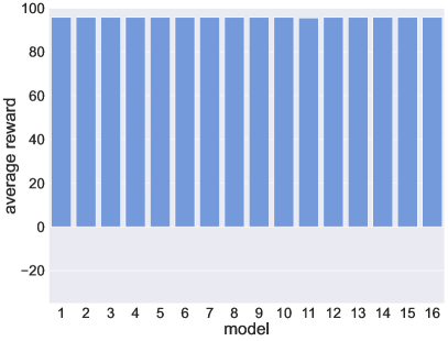
(a)

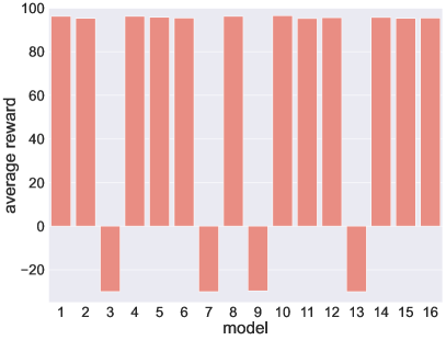
(b)

Figure 7: Mountain Car: the models’ average rewards in different distributions.

To evaluate our algorithm, we ran it on these models, and the aforementioned (OOD) input domain, and checked whether it removed the models that (although successful in-distribution) fail in the new, harder, setting. Indeed, our method was able to filter out all unsuccessful models, leaving only a subset of $5$ models ($\{2,4,8,10,15\}$), all of which perform well in the OOD scenario. For additional information, see Appendix F.

4.3 The Aurora Congestion Controller

In the third benchmark, we applied our methodology to an intricate system that enforces a policy for the real-world task of Internet congestion control. Congestion control aims to determine, for each traffic source in a communication network, the appropriate rate at which data packets should be dispatched into the network. Managing congestion is a notably challenging and fundamental issue in computer networking [53, 54]; transmitting packets too quickly can result in network congestion, causing data loss and delays. Conversely, employing low sending rates may result in the underutilization of available network bandwidth. Developed by [14], Aurora is a DNN-based congestion controller trained to optimize network performance. Recent research has delved into formally verifying the reliability of DNN-based systems, with Aurora serving as a key example [55, 56]. Within each time-step, an Aurora agent collects network statistics and determines the packet transmission rate for the next time-step. For example, if the agent observes poor network conditions (e.g., high packet loss), we expect it to decrease the packet sending rate to better utilize the bandwidth. We note that Aurora handles a much harder task than the previous RL benchmarks (Cartpole and Mountain Car): congestion controllers must gracefully respond to diverse potential events, interpreting nuanced signals presented by Aurora’s inputs. Unlike in prior benchmarks, determining the optimal policy in this scenario is not a straightforward endeavor.

Agent and Environment. Aurora receives as input an ordered set of $t$ vectors $v_{1},\ldots,v_{t}$, that collectively represent observations from the previous $t$ time-steps (each of the vectors $v_{i}\in\mathbb{R}^{3}$ includes three distinct values that represent statistics on the network’s condition, as detailed in Appendix G). The agent has a single output indicating the change in the packet sending rate over the following time-step. In line with [55, 14, 56], we set $t=10$ time-steps, hence making Aurora’s inputs of dimension $3t=30$. During training, Aurora’s reward function is a linear combination of the data sender’s packet loss, latency, and throughput, as observed by the agent (see [14] for more details).

In-Distribution Inputs. During training, Aurora executes congestion control on basic network scenarios — a single sender node sends traffic to a single receiver node across a single network link. Aurora undergoes training across a range of options for the initial sending rate, link bandwidth, link packet-loss rate, link latency, and the size of the link’s packet buffer. During the training phase, data packets are initially sent by Aurora at a rate that corresponds to $0.3-1.5$ times the link’s bandwidth, leading mostly to low congestion, as depicted in Fig. 8(a).

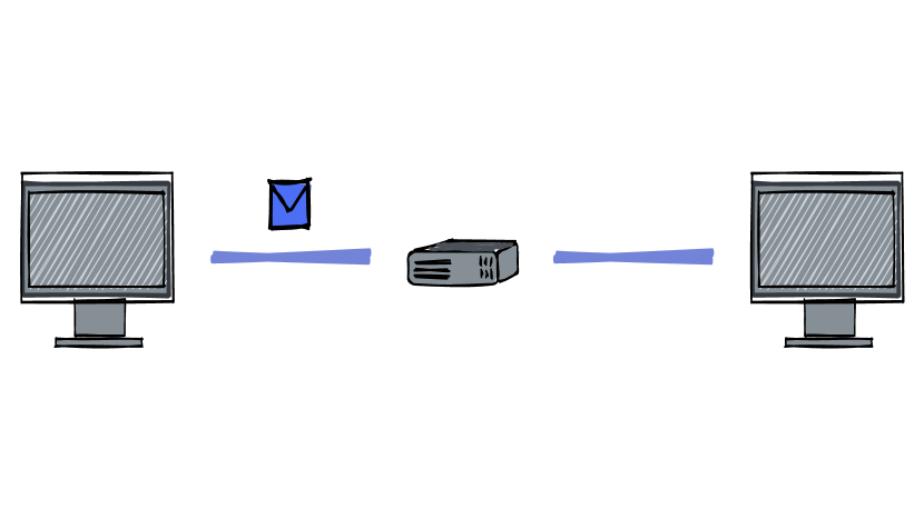
(a) In-distribution setting, in which the agent was trained, with low packet congestion

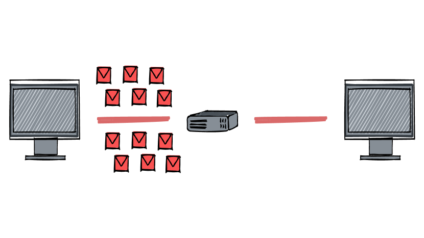
(b) OOD settings, of a much higher congestion rate, with a significantly greater packet loss

Figure 8: Aurora: illustration of in-distribution and OOD settings.

(OOD) Input Domain. In our experiments, the input domain represented a link with a limited packet buffer, indicating that the network can only store a small number of packets (with most surplus traffic being discarded), resulting in the link displaying erratic behavior. This is reflected in the initial sending rate being set to up to $8$ times (!) the link’s bandwidth, simulating the potential for a significant reduction in available bandwidth (for example, due to competition, traffic shifts, etc.). For additional details, see Appendix G.

Evaluation. We executed our algorithm and evaluated the models by assessing their disagreement upon this extensive domain, encompassing inputs that were not encountered during training, and representing the aforementioned conditions (depicted in Fig. 8(b)).

Experiment (1): High Packet Loss. In this experiment, we trained more than $100$ Aurora agents in the original (in-distribution) environment. From this pool, we chose $k=16$ agents that attained a high average reward in the in-distribution setting (see Fig. LABEL:subfig:auroraRewards:inDist), as evaluated over $40,000$ episodes from the same distribution on which the models were trained. Subsequently, we assessed these agents using out-of-distribution inputs within the previously outlined domain. The primary distinction between the training distribution and the new (OOD) inputs lies in the potential occurrence of exceptionally high packet loss rates during initialization.

Our assessment of out-of-distribution inputs within the domain reveals that while all $16$ models excelled in the in-distribution setting, only $7$ agents demonstrated the ability to effectively handle such OOD inputs (see Fig. LABEL:subfig:auroraRewards:OOD). When Algorithm 2 was applied to the $16$ models, it successfully identified and removed all $9$ models that exhibited poor generalization on the out-of-distribution inputs (see Fig. 10). Additionally, it is worth mentioning that during the initial iterations, the four models chosen for exclusion were $\{1,2,6,13\}$ — which constitute the poorest-performing models on the OOD inputs (see Appendix G).

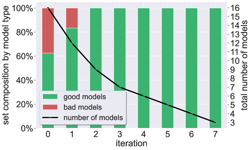
(a) OOD $\sim\mathcal{TN}(\mu_{low},\sigma^{2}$)

(b) OOD $\sim\mathcal{TN}(\mu_{high},\sigma^{2}$)

Figure 30: Aurora: Additional PDFs: model selection results for OOD values; the models are the same as in Experiment 8.

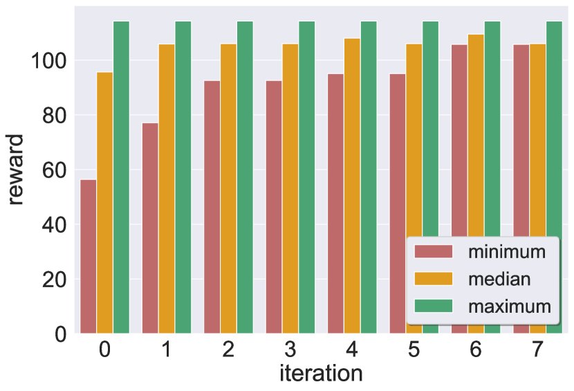
(a) OOD $\sim\mathcal{TN}(\mu_{low},\sigma^{2}$)

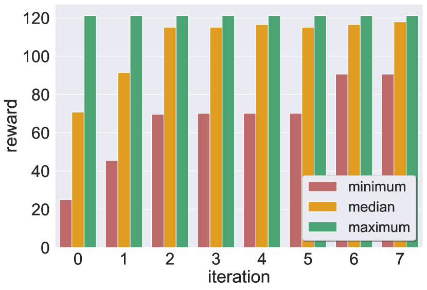
(b) OOD $\sim\mathcal{TN}(\mu_{high},\sigma^{2}$)

Figure 31: Aurora: Additional PDFs: model selection results: rewards statistics per iteration; the models are the same as in Experiment 8.

Experiment (2): Additional Distributions over OOD Inputs. To further demonstrate that our method is apt to retain superior-performing models and eliminate inferior ones within the given input domain, we conducted additional Aurora experiments by varying the distributions (probability density functions) over the OOD inputs. Our assessment indicates that all models filtered out by Algorithm 2 consistently exhibited low reward values also for these alternative distributions (see Fig. 30 and Fig. 31 in Appendix G). These results highlight an important advantage of our approach: it applies to all inputs within the considered domain, and so it applies to all distributions over these inputs. We note again that our model filtering process is based on verification queries in which the imposed bounds can represent infinitely many distribution functions, on these bounds. In other words, our method, if correct, should also apply to additional OOD settings, beyond the ones we had originally considered, which share the specified input range but may include a different probability density function (PDF) over this range.

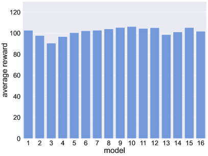
(a)

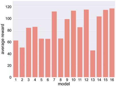
(b)

Figure 9: Aurora Experiment 8: the models’ average rewards when simulated on different distributions.

(a) Reward statistics of remaining models

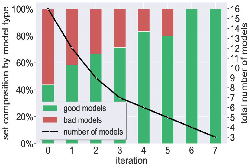
(b) Ratio between good/bad models

Figure 10: Aurora: Alg. 2’s results, per iteration. Our technique selected models {7,9,16}.

Additional Experiments. We additionally created a fresh set of Aurora models by modifying the training process to incorporate substantially longer interactions (increasing from $50$ to $400$ steps). Subsequently, we replicated the aforementioned experiments. The outcomes, detailed in Appendix G, affirm that our approach once again effectively identified a subset of models capable of generalizing well to distributions across the OOD input domain.

4.4 Arithmetic DNNs

In our last benchmark, we applied our approach to supervised-learning models, as opposed to models trained via DRL. In supervised learning, the agents are trained using inputs that have accompanying “ground truth” results, per data point. Specifically, we focused here on an Arithmetic DNNs benchmark, in which the DL models are trained to receive an input vector, and to approximate a simple arithmetic operation on some (or all) of the vector’s entries. We note that this supervised-learning benchmark is considered quite challenging [33, 34].

Agent and Environment. We trained a DNN for the following supervised task. The input is a vector of size $10$ of real numbers, drawn uniformly at random from some range $[l,u]$. The output is a single scalar, representing the sum of two hidden (yet consistent across the task) indices of the input vector; in our case, the first $2$ input indices, as depicted in Fig. 11. Differently put, the agent needs to learn to model the sum of the relevant (initially unknown) indices, while learning to ignore the rest of the inputs. We trained our networks for 10 epochs over a dataset consisting of $10,000$ input vectors drawn uniformly at random from the range $[l=-10,u=10]$, using the Adam optimization algorithm [57] with a learning rate of $\gamma=0.001$ and using the mean squared error (MSE) loss function. For additional details, see Appendix B.

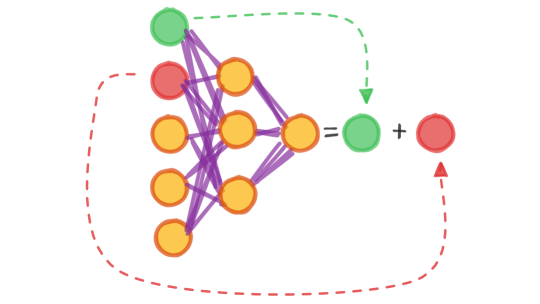
Figure 11: A toy example of a DNN that performs simple arithmetic. The DNN receives a d-dimensional input and learns to output a single value which constitutes the sum of the first two inputs of the vector, while ignoring the remaining (d-2) inputs.

In-Distribution Inputs. During training, we presented the models with input values sampled from a multi-modal uniform distribution [-10,10]¹⁰, resulting in a single output in the range [-20,20]. As expected, the models performed well over this distribution, as depicted in Fig. LABEL:subfig:arithmeticDnns:inDist of the Appendix.

(OOD) Input Domain. A natural OOD distribution includes any $d$-dimensional multi-modal distribution, in which each input is drawn from a range different than $[l=-10,u=10]$ — and hence, can necessarily be assigned values on which the model was not trained initially. In our case, we chose the multi-modal distribution of $[l=-1,000,u=1,000]$¹⁰. Unlike the case for the in-distribution inputs, there was a high variance among the performance of the models in this novel, unseen OOD setting, as depicted in Fig. LABEL:subfig:arithmeticDnns:OOD of the Appendix.

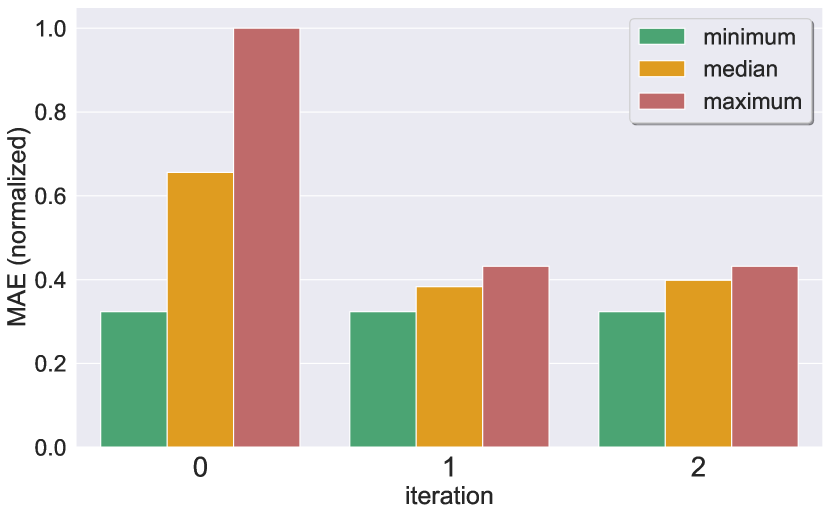
(a) MAE statistics

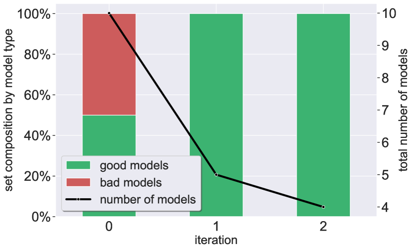
(b) Ratio between good/bad models

Figure 47: Arithmetic DNNs: results using the MAX filtering criterion, and the COMBINED filtering criterion (identical results). Our technique selected models {1,5,8,10}.

Evaluation. We originally trained $n=50$ models. After validating that all models succeed in-distribution, we generated a pool of $k=10$ models. This pool was generated by collecting the five best and five worst models OOD (based on their maximal normalized error, over the same $100,000$ points sampled OOD). We then executed our algorithm and checked whether it was able to identify and remove all unsuccessful models, which consisted of half of the original model pool. Indeed, as can be seen in Fig. 12, all bad models were filtered out within three iterations. After convergence, three models remained in the model pool, including model {8} — which constitutes the best model, OOD. This experiment was successfully repeated with additional filtering criteria (see Fig. 47 in Appendix H).

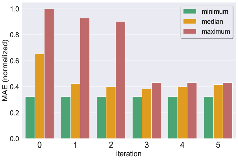
(a) MAE statistics of remaining models

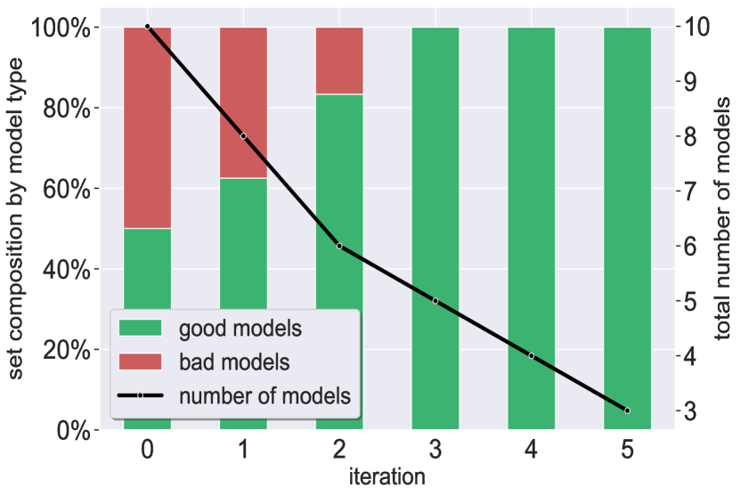
(b) Ratio between good/bad models

Figure 12: Arithmetic DNNs: Alg. 2’s results, per iteration. Our technique selected models {5,8,10}.

4.5 Averaging the Selected Models

To improve performance even further, it is possible to create (in polynomial time) an ensemble of the surviving “good” models, instead of selecting a single model. As DNN robustness is linked to uncertainty, and due to the use of ensembles as a prominent approach for uncertainty prediction, it has been shown that averaging ensembles may improve performance [58]. For example, in the Arithmetic DNNs benchmark, our approach eventually selected three models ({$5$}, {$8$}, and {$9$}, as depicted in Fig. 12). Subsequently, we generated an ensemble comprised of these three DNN models. Now, when the ensemble evaluates a given input, that input is first independently passed to each of the ensemble members; and the final ensemble prediction is the average of each of the members’ original outputs. We then sampled $5,000$ inputs drawn in-distribution (see Fig. 13(a)) and $5,000$ inputs drawn OOD (see Fig. 13(b)), and compared the average and maximal errors of the ensemble on these sampled inputs to that of its constituents. In both cases, the ensemble had a maximal absolute error that was significantly lower than each of its three constituent DNNs, as well as a lower average error (with the sole exception of the average error OOD, which was the second-smallest error, by a margin of only $0.06$). Although the use of ensembles is not directly related to our approach, it demonstrates how our technique can be extended and built upon additional robustness techniques, for improving performance even further.

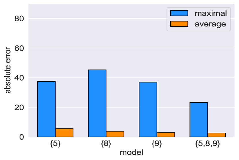
(a) In-distribution, from left to right: the maximal absolute errors are $37.44$, $45.33$, $37.01$, $23.28$, and the average absolute errors are: $5.6$, $3.84$, $2.98$, $2.65$.

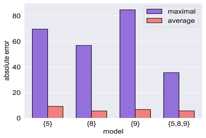
(b) OOD, from left to right: the maximal absolute errors are $69.7$, $56.9$, $84.81$, $35.59$, and the average absolute errors are: $9.23$, $5.61$, $6.77$, $5.67$.

Figure 13: Arithmetic DNNs: Ensemble results. After Alg. 2 selected models {$5$}, {$8$}, and {$9$}, we generated an ensemble {$5$,$8$,$9$} and sampled $5,000$ inputs in-distribution (a) and OOD (b). We note that we multiplied the errors attained in the in-distribution experiment by $100$ in order to normalize the selected range.

4.6 Analyzing the Eliminated Models

We conducted an additional analysis of the eliminated models, in order to compare the average PDT scores of eliminated “good” models to those of eliminated “bad” ones. For each of the five benchmarks, we divided the eliminated models into two separate clusters, of either “good” or “bad” models (note that the latter necessarily includes all bad models, as in all our benchmarks we return strictly “good” models). For each cluster, we calculated the average PDT score for all the DNN pairs. The results, summarized in Table 1, demonstrate a clear decrease in the average PDT score among the cluster of DNN pairs comprising successful models, compared to their peers. This trend is observed across all benchmarks, resulting in an average PDT score difference of between $21.2\%$ to $63.2\%$, between the clusters, per benchmark. We believe that these results further support our hypothesis that good models tend to make similar decisions.

	cartpole	mountain car	aurora (short)	aurora (long)	arithmetic
good models PDT	4	1.39	20.67	9.32	180
bad models PDT	8.44	2.08	26.22	25.3	299
ratio	47.4%	66.6%	78.8%	36.8%	60.2%

Table 1: Evaluating the eliminated models throughout all benchmarks. Columns (from left to right) represent the benchmarks: Cartpole, Mountain Car, Aurora (short training), Aurora (long training), and Arithmetic DNNs. The first row (in green) represents the average PDT score for pairs of “good” models, and the second row (in red) represents the average PDT score for pairs of “bad” models. The third row represents the ratio between the average PDT scores of both clusters, per benchmark.

5 Comparison to Gradient-Based Methods & Additional Techniques

The methods presented in this paper build upon DNN verification (e.g., Line 4 in Alg. 1) in order to solve the following optimization problem: given a pair of DNNs, an input domain, and a distance function, what is the maximal distance between their outputs? In other words, verification is rendered to find an input that maximizes the difference between the outputs of two neural networks, under certain constraints. Although DNN verification requires significant computational resources [59], nonetheless, we demonstrate that it is crucial in our setting. To support this claim, we show the results of our method when verification is replaced with other, more scalable, techniques, such as gradient-based algorithms (“attacks”) [60, 61, 62]. In recent years, these optimization techniques have become popular due to their simplicity and scalability, albeit the trade-off of inherent incompleteness and reduced precision [63, 64]. As we demonstrate next, when using gradient-based methods (instead of verification), at times, suboptimal PDT values were computed. This, in turn, resulted in retaining unsuccessful models, which were successfully removed when using DNN verification.

5.1 Comparison to Gradient-Based Methods

For our comparison, we generated three gradient attacks:

• Gradient attack # 1: a Non-Iterative Fast Gradient Sign Method (FGSM) [65] attack, used when optimizing linear constraints, e.g., $L_{1}$ norm, as in the case of Aurora and Arithmetic DNNs;

• Gradient attack # 2: an Iterative PGD [66] attack, also used when optimizing linear constraints. We note that we used this attack in cases where the previous attack failed.

• Gradient attack # 3: a Constrained Iterative PGD [66] attack, used in the case of encoding non-linear constraints (e.g., c-distance functions; see Sec. 3), as in the case of Cartpole and Mountain Car. This attack is a modified version of popular gradient attacks, that were altered in order for them to succeed in our setting.

Next, we formalize these attacks as constrained optimization problems.

5.2 Formulation

Given an input domain $\mathcal{D}$, an output space $\mathcal{O}=\mathbb{R}$, and a pair of neural networks $N_{1}:\mathcal{D}\to\mathbb{R}$ and $N_{2}:\mathcal{D}\to\mathbb{R}$, we wish to find an input $\boldsymbol{x}\in\mathcal{D}$ that maximizes the difference between the outputs of these neural networks.

Formally, in the case of the $L_{1}$ norm, we wish to solve the following optimization problem:

$$\underset{x}{\textbf{max}}\quad |N_{1}(\boldsymbol{x})-N_{2}(\boldsymbol{x})|$$

s.t. $$\boldsymbol{x}\in\mathcal{D}$$

5.2.1 Gradient Attack # $1$

In cases where only input constraints are present, a local maximum can be obtained via conventional gradient attacks, that maximize the following objective function:

$$L(\boldsymbol{x})=|N_{1}(\boldsymbol{x})-N_{2}(\boldsymbol{x})|$$

by taking steps in the direction of its gradient, and projecting them into the domain $\mathcal{D}$, that is:

$$\boldsymbol{x_{0}}\in\mathcal{D}$$

$$\boldsymbol{x}_{t+1}=[\boldsymbol{x}_{t}+\epsilon\cdot\nabla_{\boldsymbol{x}}L(\boldsymbol{x}_{t})]_{\mathcal{D}}$$

Where $[\cdot]_{\mathcal{D}}:\mathbb{R}^{n}\to\mathcal{D}$ projects the result onto $\mathcal{D}$, and $\epsilon$ being the step size. We note that $[\cdot]_{\mathcal{D}}$ may be non-trivial to implement, however for our cases, in which each input of the DNN is encoded as some range, i.e., $\mathcal{D}\equiv\{\boldsymbol{x}\ |\ x\in\mathbb{R}^{n}\,\,\forall i\in[n]:l_{i}\leq x_{i}\leq u_{i}\}$, this can be implemented by clipping every coordinate to its appropriate range, and $\boldsymbol{x_{0}}$ can be obtained by taking $\boldsymbol{x_{0}}=\frac{\boldsymbol{l}+\boldsymbol{u}}{2}$.

In our context, the gradient attacks maximize a loss function for a pair of DNNs, relative to their input. The popular FGSM attack (gradient attack # 1) achieves this by moving in a single step toward the direction of the gradient. This simple attack has been shown to be quite efficient in causing misclassification [65]. In our setting, we can formalize this (projected) FGSM as follows:

Algorithm 3 FGSM

Input: objective $L$, variables $\boldsymbol{x}$, input domain $\mathcal{D}$:(INIT, PROJECT), step size $\epsilon$
      Output: adversarial input $\boldsymbol{x}$

1:$\boldsymbol{x_{0}}\leftarrow\textsc{Init}(\mathcal{D})$

2:$\boldsymbol{x}_{\textbf{adv}}\leftarrow\textsc{Project}(\boldsymbol{x}_{0}+\epsilon\cdot\textbf{sign}(\nabla_{\boldsymbol{x}}L(\boldsymbol{x}_{0})))$

3:return $\boldsymbol{x}_{\textbf{adv}}$

In the context of our algorithms, we define $\mathcal{D}$ by two functions: INIT, which returns an initial value from $\mathcal{D}$; and PROJECT, which implements $[\cdot]_{\mathcal{D}}$.

5.2.2 Gradient Attack # $2$

A more powerful extension of this attack is the PGD algorithm, which we refer to as gradient attack # 2. This attack iteratively moves in the direction of the gradient, often yielding superior results when compared to its single-step (FGSM) counterpart. The attack can be formalized as follows:

Algorithm 4 PGD (maximize)

Input: objective $L$, variables $\boldsymbol{x}$, input domain $\mathcal{D}$:(INIT, PROJECT), iterations $T$, step size $\epsilon$
      Output: adversarial input $\boldsymbol{x}$

1:$\boldsymbol{x_{0}}\leftarrow\texttt{INIT}({\mathcal{D}})$

2:for $t=0\ldots T-1$ do

3:     $\boldsymbol{x}_{t+1}\leftarrow\texttt{PROJECT}({\boldsymbol{x}_{t}+\epsilon\cdot\nabla_{\boldsymbol{x}}L(\boldsymbol{x}_{t})})$ $\triangleright$ $\textbf{sign}(\nabla_{\boldsymbol{x}}L(\boldsymbol{x}_{t}))$ may also be used

4:end for

5:return $\boldsymbol{x}_{T}$

We note that the case for using PGD in order to minimize the objective function is symmetric.

5.2.3 Gradient Attack # $3$

In some cases, the gradient attack needs to optimize a loss function that represents constraints on the outputs of the DNN pairs as well. For example, in the case of the Cartpole and Mountain Car benchmarks, we used the c-distance function. In this scenario, we may need to encode constraints of the form:

$$N_{1}(\boldsymbol{x})\leq 0$$

$$N_{2}(\boldsymbol{x})\leq 0$$

resulting in the following constrained optimization problem:

$$\underset{x}{\textbf{max}}\quad |N_{1}(\boldsymbol{x})-N_{2}(\boldsymbol{x})|$$

s.t. $$\boldsymbol{x}\in\mathcal{D}$$

$$N_{1}(\boldsymbol{x})\leq 0$$

$$N_{2}(\boldsymbol{x})\leq 0$$

However, conventional gradient attacks are typically not geared for solving such optimizations. Hence, we tailored an additional gradient attack (gradient attack # 3) that can efficiently bridge this gap, and optimize the aforementioned constraints by combining our Iterative PGD attack with Lagrange Multipliers [67] $\boldsymbol{\lambda}\equiv(\lambda^{(1)},\lambda^{(2)})$, hence allowing to penalize solutions for which the constraints do not hold. To this end, we introduce a novel objective function:

$$L_{-}(\boldsymbol{x},\boldsymbol{\lambda})=|N_{1}(\boldsymbol{x})-N_{2}(\boldsymbol{x})|-\lambda^{(1)}\cdot\text{ReLU}(N_{1}(\boldsymbol{x}))-\lambda^{(2)}\cdot\text{ReLU}(N_{2}(\boldsymbol{x}))$$

resulting in the following optimization problem:

$$\underset{x}{\textbf{max}}\,\underset{\lambda}{\textbf{min}}\quad L_{-}(\boldsymbol{x},\boldsymbol{\lambda})$$

s.t. $$\boldsymbol{x}\in\mathcal{D}$$

$$\lambda^{(1)}\geq 0$$

$$\lambda^{(2)}\geq 0$$

Next, we implemented a Constrained Iterative PGD algorithm that approximates a solution to this optimization problem:

Algorithm 5 Constrained Iterative PGD

Input: objective $L$, input domain $\mathcal{D}$, constraints: $C_{i}(\boldsymbol{x})$, iterations: $T,T_{x},T_{\lambda}$, step sizes: $\epsilon_{x},\epsilon_{\lambda}$
      Output: adversarial input $\boldsymbol{x}$

$\boldsymbol{x_{0}}\leftarrow\textsc{Init}(\mathcal{D})$

$L_{C}(\boldsymbol{x},\boldsymbol{\lambda})\equiv L(\boldsymbol{x})-\sum^{k}_{i=0}\lambda^{(i)}\cdot\text{ReLU}(C_{i}(\boldsymbol{x}))$ $\triangleright$ the new objective

for $t=0\ldots T-1$ do

     $\boldsymbol{\lambda}_{t+1}\leftarrow\textsc{PGD\_min}(L_{C},\boldsymbol{\lambda},(\boldsymbol{\lambda}\leftarrow 0,\boldsymbol{\lambda}\geq 0),T_{\lambda},\epsilon_{\lambda})$ $\triangleright$ minimize $L_{C}(\boldsymbol{x}_{t},\boldsymbol{\lambda})$ with $\boldsymbol{x}_{t}$ as constant

     $\boldsymbol{x}_{t+1}\leftarrow\textsc{PGD\_max}(L_{C},\boldsymbol{x},\mathcal{D},T_{x},\epsilon_{x})$ $\triangleright$ maximize $L_{C}(\boldsymbol{x},\boldsymbol{\lambda}_{t})$ with $\boldsymbol{\lambda}_{t}$ as constant

end for

return $\boldsymbol{x}_{T}$

5.3 Results

We ran our algorithm on all original DRL benchmarks, with the sole difference being the replacement of the backend verification engine (Line 4 in Alg. 1) with the described gradient attacks. The first two attacks (i.e., FGSM and Iterative PGD) were used for both Aurora batches (“short” and “long” training), and the third attack (Constrained Iterative PGD) was used in the case of Cartpole and Mountain Car, as for these benchmarks we required the encoding of a distance function with constraints on the DNNs’ outputs as well. We note that in the case of Aurora, we ran the Iterative PGD attack only when the weaker attack failed (hence, only on the models from Experiment 8). Our results, summarized in Table 2, demonstrate the advantages of using formal verification, compared to competing, gradient attacks. These attacks, although scalable, resulted in various cases to suboptimal PDT values, and in turn, retained unsuccessful models that were successfully removed when using verification. For additional results, we also refer the reader to Fig. 14, Fig. 15, and Fig. 16.

ATTACK BENCHMARK FEASIBLE $\#$ PAIRS $\#$ ALIGNED $\#$ UNTIGHTENED $\#$ FAILED CRITERION SUCCESSFUL 1 Aurora (short) yes 120 70 50 0 MAX no COMBINED yes PERCENTILE yes 1 Aurora (long) yes 120 111 9 0 MAX yes COMBINED yes PERCENTILE yes 2 Aurora (short) yes 120 104 16 0 MAX no COMBINED yes PERCENTILE yes 3 Mountain Car no 120 38 35 47 MAX no COMBINED no PERCENTILE no 3 Cartpole partially 120 56 61 3 MAX no COMBINED no PERCENTILE no

Table 2: Summary of the gradient attack comparison. The first two columns describe the attack chosen and the benchmark on which it was evaluated; the third column states if the incomplete attack allowed a gradient-based approximation of all PDT scores; the next four columns respectively represent the total number of DNN pairs, the number of pairs in which the attack returned a PDT score identical to the original one received by our verification engine, the number of pairs in which the attack returned a score that is less precise than the one returned by our verification engine, and the number of cases in which that attack failed to generate outputs with both signs (however, this does not mean that it cannot succeed by relaxing the constraint and observing partial outputs). The second-to-last column states the filtering criterion, and the last column indicates whether using the attack-based scores resulted in solely successful models (as was the case when verification was used).

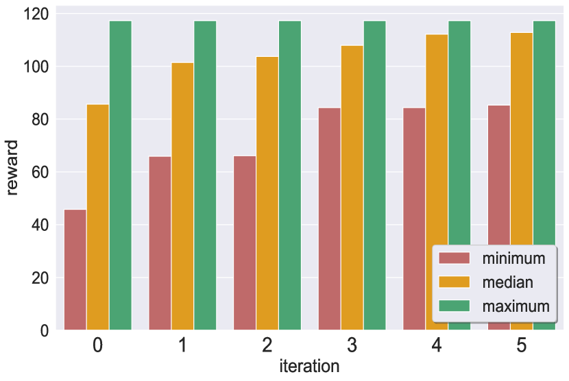
(a) Reward statistics of remaining models

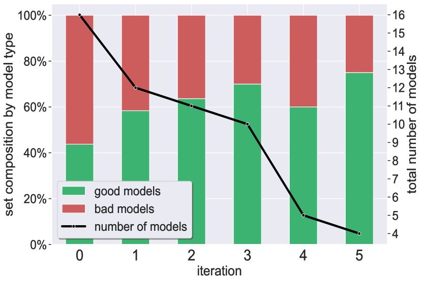
(b) Ratio between good/bad models

Figure 14: Aurora: Gradient attack # 1 (single-step FGSM): Results of models filtered using PDT scores approximated by gradient attacks (instead of a verification engine) on short-trained Aurora models, using the MAX criterion (and terminating in advance if the disagreement scores are no larger than $2$). In contrast to our verification-driven approach, the final result contains a bad model. Compare to Fig. 34.

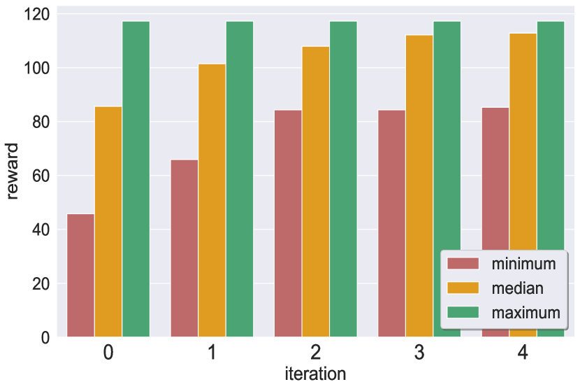
(a) Reward statistics of remaining models

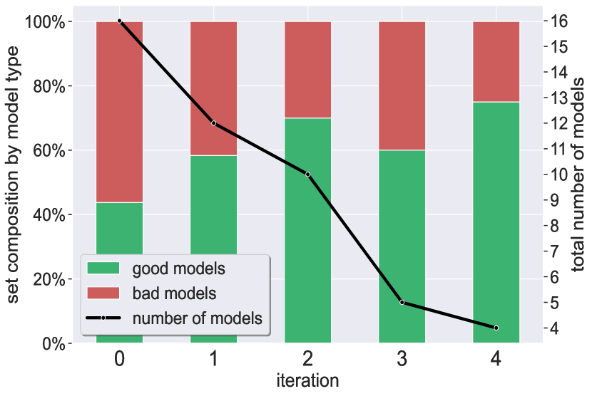
(b) Ratio between good/bad models

Figure 15: Aurora: Gradient attack # 2 (Iterative PGD): Results of models filtered using PDT scores approximated by gradient attacks (instead of a verification engine) on short-trained Aurora models, using the MAX criterion (and terminating in advance if the disagreement scores are no larger than $2$). In contrast to our verification-driven approach, the final result contains a bad model. Compare to Fig. 34.

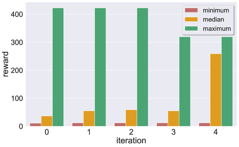
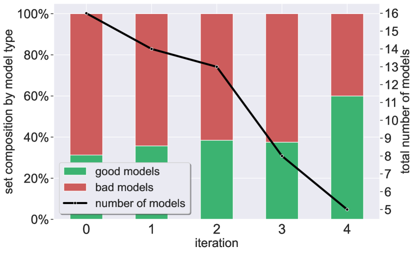
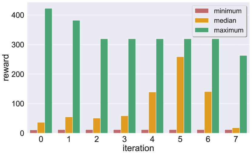
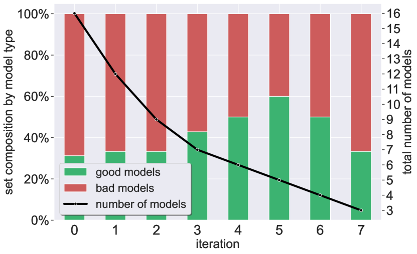
(a) Reward statistics of remaining models

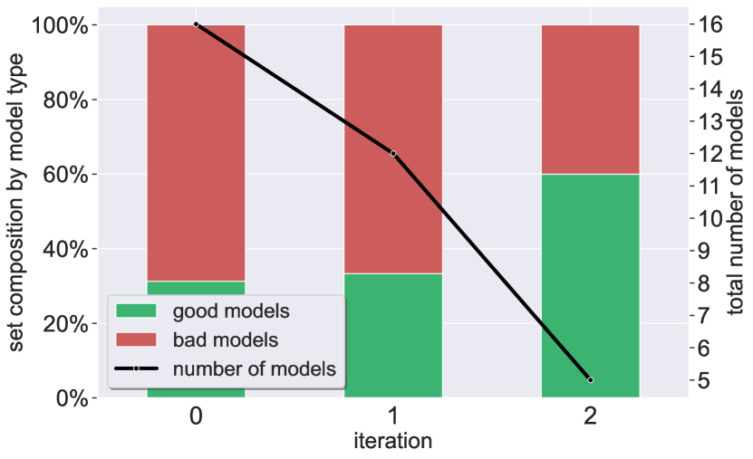
(b) Ratio between good/bad models

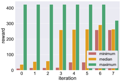
Figure 20: Cartpole: model selection results: minimum, median, and maximum rewards of the models selected after each iteration. Our technique selected models {6,7,9}.

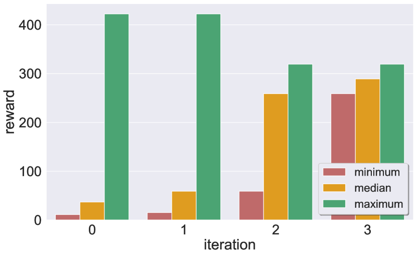
(a) Reward statistics of remaining models

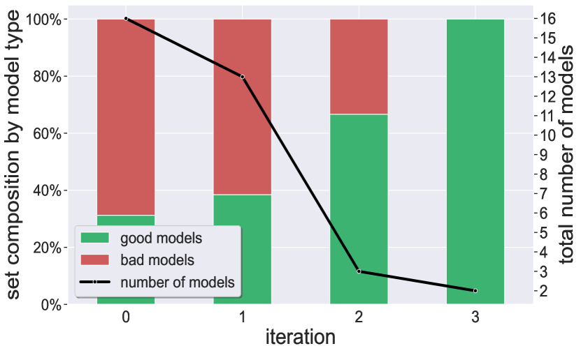
(b) Ratio between good/bad models

Figure 21: Cartpole: results using the MAX filtering criterion. Our technique selected models {7, 9}.

Figure 16: Cartpole: Gradient attack # 3 (Constrained Iterative PGD): Results of models filtered using PDT scores approximated by gradient attacks (instead of a verification engine) on the Cartpole models.
Each row, from top to bottom, contains results using a different filtering criterion (and terminating in advance if the disagreement scores are no larger than $2$): PERCENTILE (compare to Fig. 5 and Fig. 20), MAX (compare to Fig. 21), and COMBINED (compare to Fig. 22).
In all cases, the algorithm returned at least one bad model (and usually more than one), resulting in models with lower average rewards than the models returned with our verification-based approach.

5.4 Comparison to Sampling-Based Methods

In yet another line of experiments, we again replaced the verification sub-procedure of our technique, and calculated the PDT scores (Line 4 in Alg. 1) with sampling heuristics instead. We note that, as any sampling technique is inherently incomplete, this can be used solely for approximating the PDT scores. In our experiment, we sampled $1,000$ inputs from the OOD domain, and fed them to all DNN pairs, per each benchmark. Based on the outputs of the DNN pairs, we approximated the PDT scores, and ran our algorithm in order to assess if scalable sampling techniques can replace our verification-driven procedure. Our experiment raised two main concerns regarding the use of sampling techniques instead of verification.

First, in many cases, sampling could not result in constrained outputs. For instance, in the Mountain Car benchmark, we use the c-distance function (see subsec. 3.2), which requires outputs with multiple signs. However, even extensive sampling cannot guarantee this — over a third (!) of all Mountain Car DNN pairs had non-negative outputs, for all $1,000$ OOD samples, hence requiring approximation of the PDT scores even further, based only on partial outputs. On the other hand, encoding the c-distance conditions in SMT is straightforward in our case, and guarantees the required constraints.

The second setback of this approach is that, as in the case of gradient attacks, sampling may result in suboptimal PDT scores, that skew the filtering process to retain unwanted models. For example, in our results (summarized in Table 3), in both the Mountain Car and Aurora (short-training) benchmarks the algorithm returned unsuccessful (“bad”) models in some cases, while these models are effectively removed when using verification. We believe that these results further motivate the use of verification, instead of applying more scalable and simpler methods.

BENCHMARK	CRITERION	SURVIVING MODELS
Cartpole	MAX	{7}
	PERCENTILE	{6,7,9}
	COMBINED	{7,9}
Mountain Car	MAX	{1, 2, 3, 5, 6, 7, 8, 9, 10, 11, 13, 16}
	PERCENTILE	{1, 5, 8}
	COMBINED	{1, 5, 6, 8, 9, 10, 13}
Aurora (short)	MAX	{7, 9, 11, 16}
	PERCENTILE	{7, 15, 16}
	COMBINED	{7, 16}
Aurora (long)	MAX	{20, 22, 27, 28}
	PERCENTILE	{20, 27, 28}
	COMBINED	{20, 22, 27, 28}
Arithmetic DNNs	MAX	{1,5,6,8,10}
	PERCENTILE	{6, 8, 10}
	COMBINED	{1,5,6,8,10}

Table 3: A summary of Alg. 2’s results, per each of the five benchmarks: Cartpole, Mountain Car, Aurora (short & long training), and Arithmetic DNNs. For each benchmark, we sampled $1,000$ OOD inputs, and approximated the PDT scores, based on which we ran Alg. 2. The columns, from left to right, indicate the benchmark, the filtering criterion, and the surviving models, with the unsuccessful models colored in red. We note that for cases in which the c-condition was used and could not be approximated on both signs, we approximated it based on the partial results, as afforded by the sampling technique.

5.5 Comparison to Predictive Uncertainty Methods

In yet another experiment, we evaluated whether our verification-driven approach can be replaced with predictive uncertainty methods [68, 69]. These methods are online techniques, that assess uncertainty, i.e., discern whether an encountered input aligns with the training distribution. Among these techniques, ensembles [70, 71, 72] are a popular approach for predicting the uncertainty of a given input, by comparing the variance among the ensemble members; intuitively, the higher the variance is for a given input, the more “uncertain” the models are with regard to the desired output. We note that in subsec. 4.5 we demonstrate that after using our verification-driven approach, ensembling the resulting models may improve the overall performance relative to each individual member. However, now we set to explore whether ensembles can not only extend our verification-driven approach, but also replace it completely. As we demonstrate next, ensembles, like gradient attacks and sampling techniques, are not a reliable replacement for verification in our setting. For example, in the case of Cartpole, we generated all possible $k$-sized ensembles (we chose $k=3$ as this was the number of selected models via our verification-driven approach, see Fig. 5), resulting in ${n\choose k}={16\choose 3}=560$ ensemble combinations. Next, we randomly sampled $10,000$ OOD inputs (based on the specification in Appendix C) and utilized a variance-based metric (inspired by [73]) to identify ensemble subsets exhibiting low output variance on these OOD-sampled inputs. However, even the subset represented by the ensemble with the lowest variance, included the “bad” model $\{8\}$ (see Fig. 4), which was successfully removed in our equivalent verification-driven technique. We believe that this too demonstrates the merits of our verification-driven approach.

6 Related Work

Due to its widespread occurrence, the phenomenon of adversarial inputs has gained considerable attention [74, 75, 76, 77, 78, 79, 80]. Specifically, The machine learning community has dedicated substantial effort to measure and enhance the robustness of DNNs [81, 66, 82, 83, 84, 85, 86, 87, 88, 89, 90]. The formal methods community has also been looking into the problem, by devising methods for DNN verification, i.e., techniques that can automatically and formally guarantee the correctness of DNNs [43, 32, 27, 91, 92, 93, 94, 95, 96, 97, 31, 28, 98, 99, 100, 101, 102, 103, 104, 105, 106, 107, 108, 109, 110, 111, 112, 113, 114, 115, 22, 116, 117]. These techniques include SMT-based approaches (e.g., [46, 59, 49, 118]) as used in this work, methods based on MILP and LP solvers (e.g., [119, 29, 120, 121]), methods based on abstract interpretation or symbolic interval propagation (e.g., [45, 30, 122, 123]), as well as abstraction-refinement (e.g., [124, 25, 26, 27, 125, 126, 127]), size reduction [128], quantitative verification [24], synthesis [22], monitoring [21], optimization [23, 129], and also tools for verifying recurrent neural networks (RNNs) [114, 115]. In addition, efforts have been undertaken to offer verification with provable guarantees [106, 107], verification of DNN fairness [108], and DNN repair and modification after deployment [109, 110, 111, 112, 113]. We also note that some sound and incomplete techniques [130, 91] have put forth an alternative strategy for DNN verification, via convex relaxations. These techniques are relatively fast, and can also be applied by our approach, which is generally agnostic to the underlying DNN verifier. In the specific case of DRL-based systems, various non-verification approaches have been put forth to increase the reliability of such systems [131, 132, 133, 134, 135]. These techniques rely mostly on Lagrangian Multipliers [136, 137, 138].

In addition to DNN verification techniques, another approach that guarantees safe behavior is shielding [139, 140], i.e., incorporating an external component (a “shield”) that enforces the safe behavior of the agent, according to a given specification on the input/output relation of the DNN in question. Classic shielding approaches [141, 139, 140, 142, 143] focus on simple properties that can be expressed in Boolean LTL formulas. However, proposals for reactive synthesis methods within infinite theories have also emerged recently [144, 145, 146]. Yet another relevant approach is Runtime Enforcement [147, 148, 149], which is akin to shielding but incompatible with reactive systems [139]. In a broader sense, these aforementioned techniques can be viewed as part of ongoing research on improving the safety of Cyber-Physical Systems (CPS) [150, 151, 152, 153, 154].

Variability among machine learning models has been widely employed to enhance performance, often through the use of ensembles [70, 71, 72]. However, only a limited number of methodologies utilize ensembles to tackle generalization concerns [155, 156, 157, 158]. In this context, we note that our approach can also be used for additional tasks, such as ensemble selection [64], as it can identify subsets of models that have a high variance in their outputs. Furthermore, alternative techniques beyond verification for assessing generalization involve evaluating models across predefined new distributions [159].

In the context of learning, there is ample research on identifying and mitigating data drifts, i.e., changes in the distribution of inputs that are fed to the ML model, during deployment [160, 161, 162, 163, 164, 165]. In addition, certain studies employ verification for novelty detection with respect to DNNs concerning a single distribution [166]. Other work focused on applying verification to evaluate the performance of a model relative to fixed distributions [167, 168], while non-verification approaches, such as ensembles [155, 156, 157, 158], runtime monitoring [166], and other techniques [159], have been applied for OOD input detection. Unlike the aforementioned approaches, our objective is to establish verification-guided generalization scores that encompass an input domain, spanning multiple distributions within this domain. Furthermore, as far as we are aware, our approach represents the first endeavor to harness the diversity among models to distill a subset with enhanced generalization capabilities. Particularly, it is also the first endeavor to apply formal verification for this goal.

7 Limitations

Although our evaluation results indicate that our approach is applicable to varied settings and problem domains, it may suffer from multiple limitations. First, by design, our approach assumes a single solution to a given generalization problem. This does not allow selecting DNNs with different generalization strategies to the same problem. We also note that although our approach builds upon verification techniques, it cannot assure correctness or generalization guarantees of the selected models (although, in practice, this can happen in various scenarios — as our evaluation demonstrates).

In addition, our approach relies on the underlying assumption that the range of inputs is known apriori. In some situations, this assumption may turn out to be highly non-trivial — for example, in cases where the DNN’s inputs are themselves produced by another DNN, or some other embedding mechanism. Furthermore, even when the range of inputs is known, bounding their exact values may require domain-specific knowledge for encoding various distance functions, and the metrics that build upon them (e.g., PDT scores). For example, in the case of Aurora, routing expertise is required in order to translate various Internet congestion levels to actual bounds on Aurora’s input variables. We note that such knowledge may be highly non-trivial in various domains.

Finally, we note that other limitations stem from the use of the underlying DNN verification technology, which may serve as a computational bottleneck. Specifically, while our approach requires dispatching a polynomial number of DNN verification queries, solving each of these queries is NP-complete [43]. In addition, the underlying DNN verifier itself may limit the type of encodings it affords, which, in turn, restricts various use-cases to which our approach can be applied. For example, sound and complete DNN verification engines are currently suitable solely for DNNs encompassing piecewise-linear activations. However, as DNN verification technology improves, so will our approach.

8 Conclusion

This case study presents a novel, verification-driven approach to identify DNN models that effectively generalize to an input domain of interest. We introduced an iterative scheme that utilizes a backend DNN verifier, enabling us to assess models by scoring their capacity to generate similar outputs for multiple distributions over a specified domain. We extensively evaluated our approach on multiple benchmarks of both supervised, and unsupervised learning, and demonstrated that, indeed, it is able to effectively distill models capable of successful generalization capabilities. As DNN verification technology advances, our approach will gain scalability and broaden its applicability to a more diverse range of DNNs.

Declarations

We made use of Large Language Models (LLMs) for assistance in rephrasing certain parts of the text. We do not have further disclosures or declarations.

Appendices

Appendix A DRL Benchmarks: Training and Evaluation

In this appendix, we elaborate on the hyperparameters and the training procedure, for reproducing all models and environments of all three DRL benchmarks. We also provide a thorough overview of various implementation details. The code is based on the Stable-Baselines 3 [169] and OpenAI Gym [170] packages. Unless stated otherwise, the values of the various parameters used during training and evaluation are the default values (per training algorithm, environment, etc.).

A.1 Training Algorithm

We trained our models with Actor-Critic algorithms. These are state-of-the-art RL training algorithms that iteratively optimize two neural networks:

• a critic network, that learns a value function [10] (also known as a Q-function), that assigns a value to each $\langle$state,action$\rangle$ pair; and

• an actor network, which is the DRL-based agent trained by the algorithm. This network iteratively maximizes the value function learned by the critic, thus improving the learned policy.

Specifically, we used two implementations of Actor-Critic algorithms: Proximal Policy Optimization (PPO) [39] and Soft Actor-Critic (SAC) [42].

Actor-Critic algorithms are considered very advantageous, due to their typical requirement of relatively few samples to learn from, and also due to their ability to allow the agent to learn policies for continuous spaces of $\langle$state,action$\rangle$ pairs.

In each training process, all models were trained using the same hyperparameters, with the exception of the Pseudo Random Number Generator’s (PRNG) seed. Each training phase consisted of $10$ checkpoints, while each checkpoint included a constant number of environment steps, as described below. For model evaluation, we used the last checkpoint of each training process (per benchmark).

A.2 Architecture

In all benchmarks, we used DNNs with a feed-forward architecture. We refer the reader to Table 4 for a summary of the chosen architecture per each benchmark.

benchmark	hidden layers	layer size	activation function	training algorithm
Cartpole	2	[32, 16]	ReLU	PPO
Mountain Car	2	[64, 16]	ReLU	SAC
Aurora	2	[32, 16]	ReLU	PPO

Table 4: DNN architectures and training algorithms, per benchmark.

A.3 Cartpole Parameters

A.3.1 Architecture and Training

1. Architecture

   • hidden layers: 2

   • size of hidden layers: 32 and 16, respectively

   • activation function: ReLU

2. Training

   • algorithm: Proximal Policy Optimization (PPO)

   • gamma ($\gamma$): 0.95

   • batch size: 128

   • number of checkpoints: $10$

   • total time-steps (number of training steps for each checkpoint): $50,000$

   • PRNG seeds (each one used to train a different model):
     $\{1,2,3,4,5,6,7,8,9,10,11,12,13,14,15,16\}$

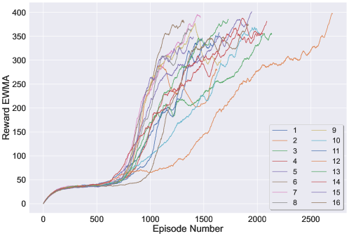
Figure 17: Cartpole: models’ exponential weighted moving average (EWMA) reward during training. All models achieved a high reward (at the end of their training phase).

A.3.2 Environment

We used the configurable CartPoleContinuous-v0 environment. Given lower and upper bounds for the x-axis location, denoted as $[low,high]$, and $mid=\frac{high+low}{2}$, the initial x position is randomly, uniformly drawn from the interval $[mid-0.05,mid+0.05]$.

An episode is a sequence of interactions between the agent and the environment, such that the episode ends when a terminal state is reached. In the Cartpole environment, an episode terminates after the first of the following occurs:

1. The cart’s location exceeds the platform’s boundaries (as expressed via the $x$-axis location); or

2. The cart was unable to balance the pole, which fell (as expressed via the $\theta$-value); or

3. $500$ time-steps have passed.

A.3.3 Domains

1. (Training) In-Distribution

   • action min magnitude: True

   • x-axis lower bound (x_threshold_low): $-2.4$

   • x-axis upper bound (x_threshold_high): $2.4$

2. (OOD) Input Domain

   Two symmetric OOD scenarios were evaluated: the cart’s $x$ position represented significantly extended platforms in a single direction, hence, including areas previously unseen during training. Specifically, we generated a domain of input points characterized by $x$-axis boundaries that were selected, with an equal probability, either from $[-10,-2.4]$ or from $[2.4,10]$ (instead of the in-distribution range of $[-2.4,2.4])$. The cart’s initial location was uniformly drawn from the range’s center $\pm 0.05$: $[-6.4-0.05,-6.4+0.05]$ and $[6.4-0.05,6.4+0.05]$, respectively. All other parameters were the same as the ones used in-distribution.

   OOD scenario 1

   • x-axis lower bound (x_threshold_low): $-10.0$

   • x-axis upper bound (x_threshold_high): $-2.4$

   OOD scenario 2

   • x-axis lower bound (x_threshold_low): $2.4$

   • x-axis upper bound (x_threshold_high): $10.0$

A.4 Mountain Car Parameters

A.4.1 Architecture and Training

1. Architecture

   • hidden layers: 2

   • size of hidden layers: 64 and 16, respectively

   • activation function: ReLU

   • clip mean parameter: 5.0

   • log stdinit parameter: -3.6

2. Training

   • algorithm: Soft Actor-Critic (SAC)

   • gamma ($\gamma$): 0.9999

   • batch size: 512

   • buffer size: 50,000

   • gradient steps: 32

   • learning rate: $3\text{\times}{10}^{-4}$

   • learning starts: 0

   • tau ($\tau$): 0.01

   • train freq: 32

   • use sde: True

   • number of checkpoints: $10$

   • total time-steps (number of training steps for each checkpoint): $5,000$

   • PRNG seeds (each one used to train a different model):
     $\{1,2,3,4,5,6,7,8,9,10,11,12,13,14,15,16\}$

Figure 18: Mountain Car: models’ exponential weighted moving average (EWMA) reward during training. All models achieved a high reward (at the end of their training phase).

A.4.2 Environment

We used the MountainCarContinuous-v1 environment.

A.4.3 Domains

1. (Training) In-Distribution

   • min position: $-1.2$

   • max position: $-0.6$

   • goal position: $0.45$

   • min action (if the agent’s action is negative and under this value, this value is used): $-2$

   • max action (if the agent’s action is positive and above this value, this value is used): $2$

   • max speed: $0.4$

   • initial location range (from which the initial location is uniformly drawn): $[-0.9,-0.6]$

   • initial velocity range (from which the initial velocity is uniformly drawn): $[0,0]$ (i.e., the initial velocity in this scenario is always $0$)

   • x scale factor (used for scaling the x-axis): $1.5$

2. (OOD) Input Domain

   The inputs are the same as the ones used in-distribution, except for the following:

   • min position: $-2.4$

   • max position: $1.2$

   • goal position: $0.9$

   • initial location range: $[0.4,0.5]$

   • initial location velocity: $[-0.4,-0.3]$

A.5 Aurora Parameters

A.5.1 Architecture and Training

1. Architecture

   • hidden layers: 2

   • size of hidden layers: 32 and 16, respectively

   • activation function: ReLU

2. Training

   • algorithm: Proximal Policy Optimization (PPO)

   • gamma ($\gamma$): 0.99

   • number of steps to run for each environment, per update (n_steps): $8,192$

   • number of epochs when optimizing the surrogate loss (n_epochs): $4$

   • learning rate: $1\text{\times}{10}^{-3}$

   • value function loss coefficient (vf_coef): $1$

   • entropy function loss coefficient (ent_coef): $1\text{\times}{10}^{-2}$

   • number of checkpoints: $6$

   • total time-steps (number of training steps for each checkpoint): $656,000$ (as used in the original paper [14])

   • PRNG seeds (each one used to train a different model):
     $\{4,52,105,666,850,854,857,858,885,897,901,906,907,929,944,945\}$
     We note that for simplicity, these were mapped to indices $\{1\ldots 16\}$, accordingly (e.g., $\{4\}\rightarrow\{1\}$, $\{52\}\rightarrow\{2\}$, etc.).

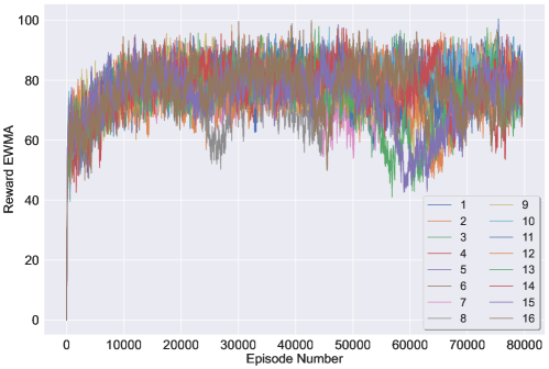
Figure 19: Aurora (short training): models’ exponential weighted moving average (EWMA) reward during training. All models achieved a high reward (at the end of their training phase).

A.5.2 Environment

We used a configurable version of the PccNs-v0 environment. For models in Exp. 8 (with the short training), each episode consisted of $50$ steps. For models in Exp. G.1 (with the long training), each episode consisted of $400$ steps.

A.5.3 Domains

1. (Training) In-Distribution

   • minimal initial sending rate ratio (to the link’s bandwidth) (min_initial_send_rate_bw_ratio): $0.3$

   • maximal initial sending rate ratio (to the link’s bandwidth) (max_initial_send_rate_bw_ratio): $1.5$

2. (OOD) Input Domain

   To bound the latency gradient and latency ratio elements of the input, we used a shallow buffer setup, with a bounding parameter $\delta>0$ such that latency gradient $\in[-\delta,\delta]$ and latency ratio $\in[1.0,1.0+\delta]$.

   • minimal initial sending rate ratio (to the link’s bandwidth) (min_initial_send_rate_bw_ratio): $2.0$

   • maximal initial sending rate ratio (to the link’s bandwidth) (max_initial_send_rate_bw_ratio): $8.0$

   • use shallow buffer: True

   • shallow buffer $\delta$ bound parameter: $1\text{\times}{10}^{-2}$

Appendix B Arithmetic DNNs: Training and Evaluation

In this appendix, we elaborate on the hyperparameters and the training procedure, for reproducing all models and environments of the supervised learning Arithmetic DNNs benchmark. We also provide a thorough overview of various implementation details.

To train our neural networks we used the pyTorch package, version $2.0.1$. Unless stated otherwise, the values of the various parameters used during training and evaluation are the default values (per training algorithm, environment, etc.).

B.1 Training Algorithm

We trained our models with the Adam optimizer [57], for $10$ epochs, and with a batch size of $32$. All models were trained using the same hyperparameters, with the exception of the Pseudo Random Number Generator’s (PRNG) seed.

B.2 Architecture

In all benchmarks, we used DNNs with a fully connected feed-forward architecture with ReLU activations.

benchmark	hidden layers	layer size	activation function	training algorithm
Arithmetic DNNs	3	[10, 10, 10]	ReLU	Adam

Table 5: Arithmetic DNNs: benchmark parameters.

B.3 Arithmetic DNNs Parameters

B.3.1 Architecture and Training

1. Architecture

   • hidden layers: 3

   • size of (each) hidden layer: 10

   • activation function: ReLU

2. Training

   • algorithm: Adam [57]

   • learning rate: $\gamma=0.001$

   • batch size: 32

   • PRNG seeds (each one used to train a different model): $[0,49]$. The $5$ models with the best seeds OOD are (from best to worse): $\{37,4,22,20,47\}$, and the $5$ models with the worst seeds OOD are (from best to worse): $\{15,12,11,44,30\}$. We note that for simplicity, these were mapped to indices $\{1\ldots 10\}$, based on their order (e.g., $\{4\}\rightarrow\{1\}$, $\{11\}\rightarrow\{2\}$, etc.).

   • loss function: mean squared error (MSE)

B.3.2 Domains

1. (Training) In-Distribution We have generated a dataset of $10,000$ vectors of dimension $d=10$, in which every entry is sampled from the multi-modal uniform distribution $[l=-10,u=10]^{10}$. Hence, $x_{1},x_{2},...,x_{10000}\sim[-10,10]^{10}$. and the output label is $y_{i}=x_{i}[0]+x_{i}[1]$.The random seed used for generating the dataset is $0$.

2. (OOD) Input Domain We evaluated our networks on $100,000$ input vectors of dimension $d=10$, where every entry is uniformly distributed between $[l=-1,000,u=1,000]$. All other parameters were identical to the ones used in-distribution.

Appendix C Verification Queries: Additional Details

C.1 Precondition

In our experiments, we used the following bounds for the (OOD) input domain:

1. Cartpole:

   • x position: $x\in[-10,-2.4]$ or $x\in[2.4,10]$ The PDT was set to be the maximum PDT score of each of these two scenarios.

   • $x$ velocity: $v_{x}\in[-2.18,2.66]$

   • angle: $\theta\in[-0.23,0.23]$

   • angular velocity: $v_{\theta}\in[-1.3,1.22]$

2. Mountain Car:

   • x position: $x\in[-2.4,0.9]$

   • $x$ velocity: $v_{x}\in[-0.4,0.134]$

3. Aurora:

   • latency gradient: $x_{t}\in[-0.007,0.007]$, for all $t$ s.t. $(t\mod 3)=0$

   • latency ratio: $x_{t}\in[1,1.04]$, for all $t$ s.t. $(t\mod 3)=1$

   • sending ratio: $x_{t}\in[0.7,8]$, for all $t$ s.t. $(t\mod 3)=2$

4. Arithmetic DNNs:

   • for all $0\leq i\leq 9$: $x_{i}\in[-1000,1000]$

C.2 Postcondition

As elaborated in subsection 3.2, we encode an appropriate distance function on the DNNs’ outputs.

Note. In the case of the c-distance function, we chose, for Cartpole and Mountain Car, $c:=N_{1}(x)\geq 0\wedge N_{2}(x)\geq 0$ and $c^{\prime}:=N_{1}(x)\leq 0\wedge N_{2}(x)\leq 0$. This distance function is tailored to find the maximal difference between the outputs (actions) of two models, in a given category of inputs (non-positive or non-negative, in our case). The intuition behind this function is that in some benchmarks, good and bad models may differ in the sign (rather than only the magnitude) of their actions. For example, consider a scenario of the Cartpole benchmark where the cart is located on the “edge” of the platform: an action in one direction (off the platform) will cause the episode to end, while an action in the other direction will allow the agent to increase its reward by continuing the episode, and possibly reaching the goal.

C.3 Verification Engine

All queries were dispatched to Marabou [49, 50] — a sound and complete verification engine, previously used in other DNN-verification-related work [64, 171, 172, 173, 115, 63, 45, 27, 124, 126, 174, 175, 56, 176, 177, 178, 179].

Appendix D Algorithm Variations and Hyperparameters

In this appendix, we elaborate on our algorithms’ additional hyperparameters and filtering criteria, used throughout our evaluation. As the results demonstrate, our method is highly robust in a myriad of settings.

D.1 Precision

For each benchmark and each experiment, we arbitrarily selected $k$ models which reached our reward threshold for the in-distribution data. Then, we used these models for our empirical evaluation. The PDT scores were calculated up to a finite precision of $0.5\leq\epsilon\leq 20$, depending on the benchmark ($0.5$ for Mountain Car, $1$ for Cartpole and Aurora, and $20$ for Arithmetic DNNs).

D.2 Filtering Criteria

As elaborated in Sec. 3, our algorithm iteratively filters out (Line 9 in Alg. 2) models with a relatively high disagreement score, i.e., models that may disagree with their peers in the input domain. We present three different criteria based on which we may select the models to remove in a given iteration, after sorting the models based on their DS score:

1. PERCENTILE: in which we remove the top $p\%$ of models with the highest disagreement scores, for a predefined value $p$. In our experiments, we chose $p=25\%$.

2. MAX: in which we:

   1. sort the DS scores of all models in a descending order;

   2. calculate the difference between every two adjacent scores;

   3. search for the greatest difference of any two subsequent DS scores;

   4. for this difference, use the larger DS as a threshold; and

   5. remove all models with a DS that is greater than or equal to this threshold.

3. COMBINED: in which we remove models based either on MAX or PERCENTILE, depending on which criterion eliminates more models in a specific iteration.

Appendix E Cartpole: Supplementary Results

Throughout our evaluation of this benchmark, we use a threshold of 250 to distinguish between good and bad models — this threshold value induces a large margin from rewards pertaining to poorly-performing models (which usually reached rewards lower than $100$).

Note that as seen in Fig. 5, our algorithm eventually also removes some of the more successful models. However, the final result contains only well-performing models, as in the other benchmarks.

E.1 Result per Filtering Criteria

(a) Reward statistics of remaining models

(b) Ratio between good/bad models

Figure 22: Cartpole: results using the COMBINED filtering criterion. Our technique selected models {7, 9}.

Appendix F Mountain Car: Supplementary Results

F.1 The Mountain Car Benchmark

We note that our algorithm is robust to various hyperparameter choices, as demonstrated in Fig. 23, Fig. 24 and Fig. 25 which depict the results of each iteration of our algorithm, when applied with different filtering criteria (elaborated in Appendix D).

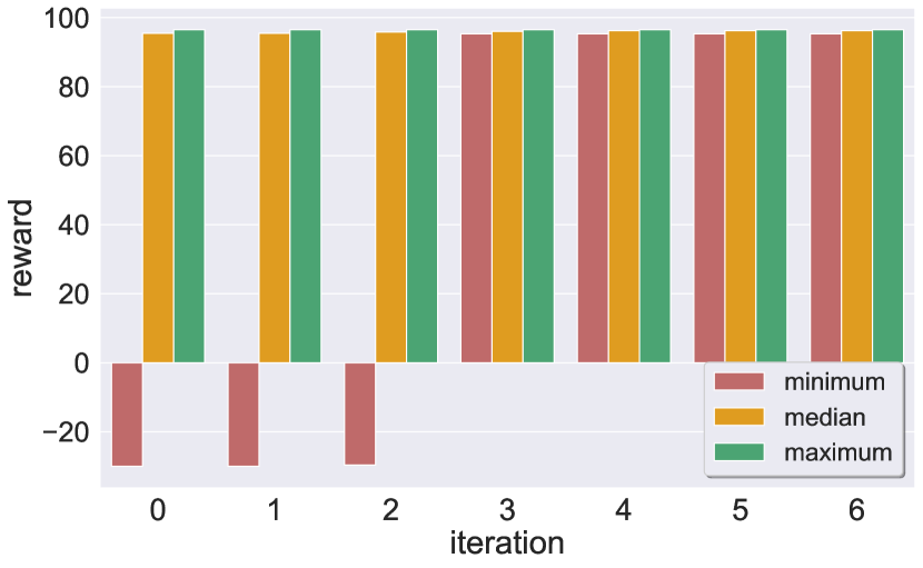
(a) Reward statistics of remaining models

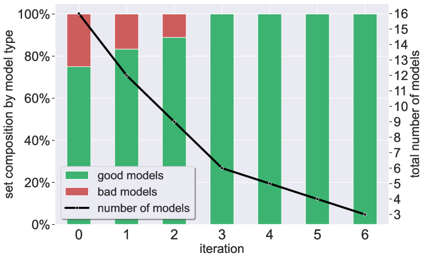
(b) Ratio between good/bad models

Figure 23: Mountain Car: results using the PERCENTILE filtering criterion. Our technique selected models {8, 10, 15}.

F.2 Additional Filtering Criteria

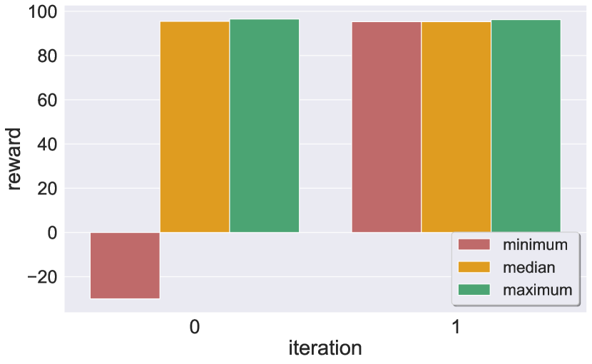
(a) Reward statistics of remaining models

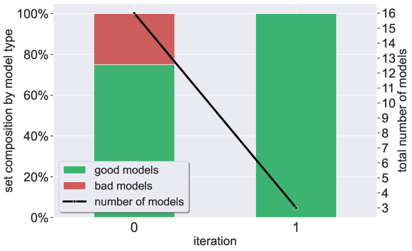
(b) Ratio between good/bad models

Figure 24: Mountain Car: results using the MAX filtering criterion. Our technique selected models {2, 4, 15}.

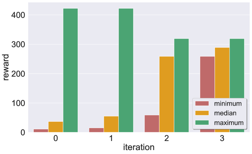
(a) Reward statistics of remaining models

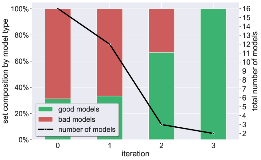
(b) Ratio between good/bad models

Figure 25: Mountain Car: results using the COMBINED filtering criterion. Our technique selected models {2, 4, 15}.

F.3 Combinatorial Experiments

Due to the original bias of the initial set of candidates, in which $12$ out of the original $16$ models are good in the OOD setting, we set out to validate that the fact that our algorithm succeeded in returning solely good models is indeed due to its correctness, and not due to the inner bias among the set of models, to contain good models. In our experiments (summarized below) we artificially generated new sets of models in which the ratio of good models is deliberately lower than in the original set. We then reran our algorithm on all possible combinations of the initial subsets, and calculated (for each subset) the probability of selecting a good model in this new setting, from the models surviving our filtering process. As we show, our method significantly improves the chances of selecting a good model even when these are a minority in the original set. For example, the leftmost column of Fig. 26 shows that over sets consisting of $4$ bad models and only $2$ good ones, the probability of selecting a good model after running our algorithm is over $60\%$ (!) — almost double the probability of randomly selecting a good model from the original set before running our algorithm. These results were consistent across multiple subset sizes, and with various filtering criteria.

Note. For the calculations demonstrating the chance to select a good model, we assume random selection from a subset of models: before applying our algorithm, the subset is the original set of models; and after our algorithm is applied — the subset is updated based on the result of our filtering procedure. The probability is computed based on the number of combinations of bad models surviving the filtering process, and their ratio relative to all the models returned in those cases (we assume uniform probability, per subset).

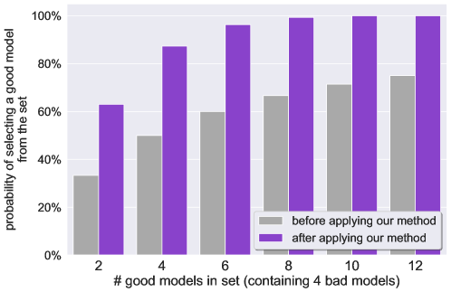
Figure 26: Mountain Car: our algorithm effectively increases the probability to choose a good model, due to effective filtering. The plot corresponds to Table 7.

COMPOSITION		total $\#$ experiments	$\#$ experiments with		probability to choose good models
good	bad	subgroup combinations of good models	all surviving models good	some surviving models bad	naive	our method
12	4	${12\choose{\color[rgb]{0,0.4296875,0.19921875}12}}=1$	1	0	75 %	100%
10	4	${12\choose{\color[rgb]{0,0.4296875,0.19921875}10}}=66$	65	1	71.43 %	99.49 %
8	4	${12\choose{\color[rgb]{0,0.4296875,0.19921875}8}}=495$	423	72	66.67 %	95.15 %
6	4	${12\choose{\color[rgb]{0,0.4296875,0.19921875}6}}=924$	549	375	60 %	86.26 %
4	4	${12\choose{\color[rgb]{0,0.4296875,0.19921875}4}}=495$	123	372	50 %	74.01 %
2	4	${12\choose{\color[rgb]{0,0.4296875,0.19921875}2}}=66$	66	0	33.33 %	54.04 %

Table 6: Results summary of the combinatorial Mountain Car experiment, using the PERCENTILE filtering criterion.

COMPOSITION		total $\#$ experiments	$\#$ experiments with		probability to choose good models
good	bad	subgroup combinations of good models	all surviving models good	some surviving models bad	naive	our method
12	4	${12\choose{\color[rgb]{0,0.4296875,0.19921875}12}}=1$	1	0	75 %	100%
10	4	${12\choose{\color[rgb]{0,0.4296875,0.19921875}10}}=66$	66	0	71.43 %	100 %
8	4	${12\choose{\color[rgb]{0,0.4296875,0.19921875}8}}=495$	486	9	66.67 %	99.34 %
6	4	${12\choose{\color[rgb]{0,0.4296875,0.19921875}6}}=924$	844	80	60 %	96.33 %
4	4	${12\choose{\color[rgb]{0,0.4296875,0.19921875}4}}=495$	375	120	50 %	87.32 %
2	4	${12\choose{\color[rgb]{0,0.4296875,0.19921875}2}}=66$	31	35	33.33 %	63.03 %

Table 7: Results summary of the combinatorial Mountain Car experiment, using the MAX filtering criterion.

COMPOSITION		total $\#$ experiments	$\#$ experiments with		probability to choose good models
good	bad	subgroup combinations of good models	all surviving models good	some surviving models bad	naive	our method
12	4	${12\choose{\color[rgb]{0,0.4296875,0.19921875}12}}=1$	1	0	75 %	100%
10	4	${12\choose{\color[rgb]{0,0.4296875,0.19921875}10}}=66$	66	0	71.43 %	100 %
8	4	${12\choose{\color[rgb]{0,0.4296875,0.19921875}8}}=495$	481	12	66.67 %	99.26 %
6	4	${12\choose{\color[rgb]{0,0.4296875,0.19921875}6}}=924$	842	82	60 %	96.74 %
4	4	${12\choose{\color[rgb]{0,0.4296875,0.19921875}4}}=495$	372	123	50 %	88.09 %
2	4	${12\choose{\color[rgb]{0,0.4296875,0.19921875}2}}=66$	31	35	33.33 %	63.36 %

Table 8: Results summary of the combinatorial Mountain Car experiment, using the COMBINED filtering criterion.

Appendix G Aurora: Supplementary Results

G.1 Additional Information

1. A detailed explanation of Aurora’s input statistics: (i) Latency Gradient: a derivative of latency (packet delays) over the recent MI (“monitor interval”); (ii) Latency Ratio: the ratio between the average latency in the current MI to the minimum latency previously observed; and (iii) Sending Ratio: the ratio between the number of packets sent to the number of acknowledged packets over the recent MI. As mentioned, these metrics indicate the link’s congestion level.

2. For all our experiments on this benchmark, we defined “good” models as models that achieved an average reward greater/equal to a threshold of 99; “bad” models are models that achieved a reward lower than this threshold.

3. In-distribution, the average reward is not necessarily correlated with the average reward OOD. For example, in Exp. 8 with the short episodes during training (see Fig. 9):

   1. In-distribution, model $\{4\}$ achieved a lower reward than models $\{2\}$ and $\{5\}$, but a higher reward OOD.

   2. In-distribution, model $\{16\}$ achieved a lower reward than model $\{15\}$, but a higher reward OOD.

Experiment (3): Aurora: Long Training Episodes

Similar to Experiment 8, we trained a new set of $k=16$ agents. In this experiment, we increased each training episode to consist of $400$ steps (instead of $50$, as in the “short” training). The remaining parameters were identical to the previous setup in Experiment 8. This time, $5$ models performed poorly in the OOD environment (i.e., did not reach our reward threshold of $99$), while the remaining $11$ models performed well both in-distribution and OOD.

When running our method with the MAX criterion, our algorithm returned $4$ models, all being a subset of the group of $11$ models which generalized successfully, and after fully filtering out all the unsuccessful models. Running the algorithm with the PERCENTILE or the COMBINED criteria also yielded a subset of this group, indicating that the filtering process was again successful (and robust to various algorithm hyperparameters).

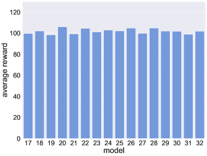
(a)

(b)

Figure 27: Aurora Experiment G.1: the models’ average rewards when simulated on different distributions.

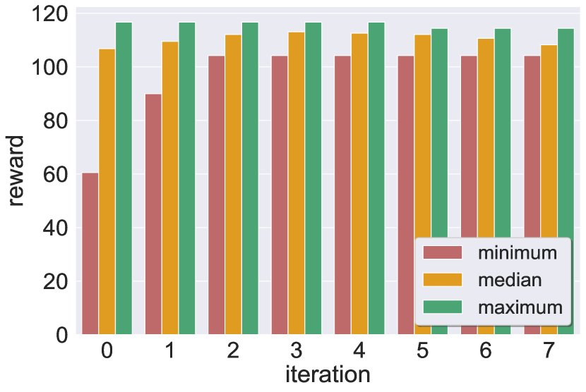
(a) Reward statistics of remaining models

(b) Ratio between good/bad models

Figure 28: Aurora Experiment G.1: model selection results. Our technique selected models {20, 27, 28}.

G.2 Additional Probability Density Functions

Following are the results discussed in subsection 4.3. To further demonstrate our method’s robustness to different types of out-of-distribution inputs, we applied it not only to different values (e.g., high Sending Rate values) but also to various probability density functions (PDFs) of values in the (OOD) input domain in question. More specifically, we repeated the OOD experiments (Experiment 8 and Experiment G.1) with different PDFs. In their original settings, all of the environment’s parameters (link’s bandwidth, latency, etc.) are uniformly drawn from a range $[low,high]$. However, in this experiment, we generated two additional PDFs: Truncated normal (denoted as $\mathcal{TN}_{[low,high]}(\mu,\sigma^{2})$) distributions that are truncated within the range $[low,high]$. The first PDF was used with $\mu_{low}=0.3*high+(1-0.3)*low$, and the other with $\mu_{high}=0.8*high+(1-0.8)*low$. For both PDFs, the variance ($\sigma^{2}$) was arbitrarily set to $\frac{high-low}{4}$. These new distributions are depicted in Fig. 29 and were used to test the models from both batches of Aurora experiments (Experiments 8 and G.1).

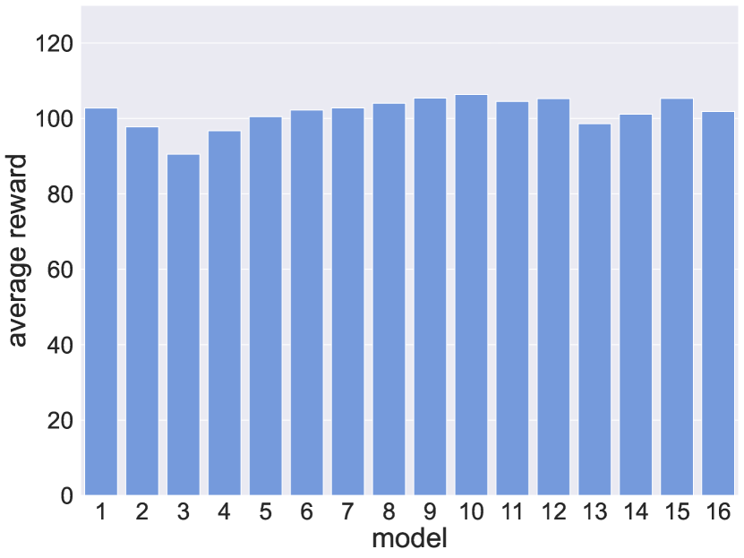
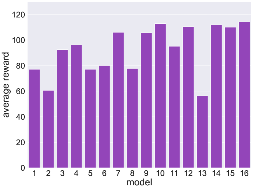
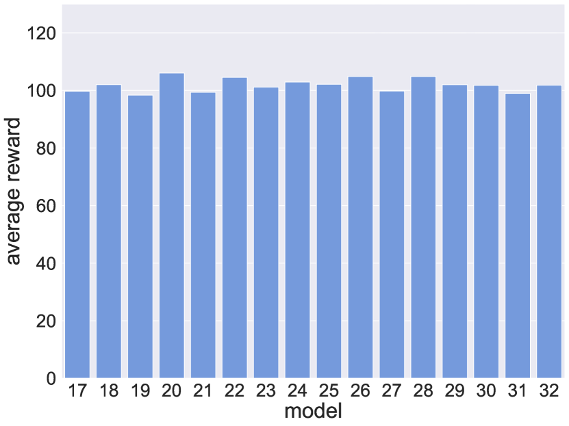
(a) In-distribution
($\sim\mathcal{U}(low,high)$)

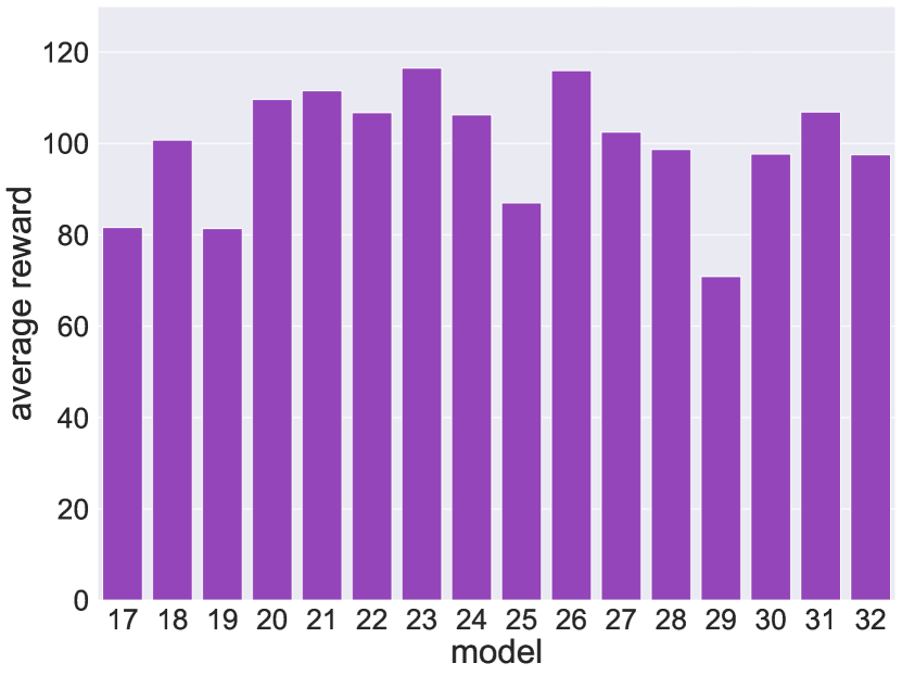
(b) OOD ($\sim\mathcal{TN}(\mu_{low},\sigma^{2}$))

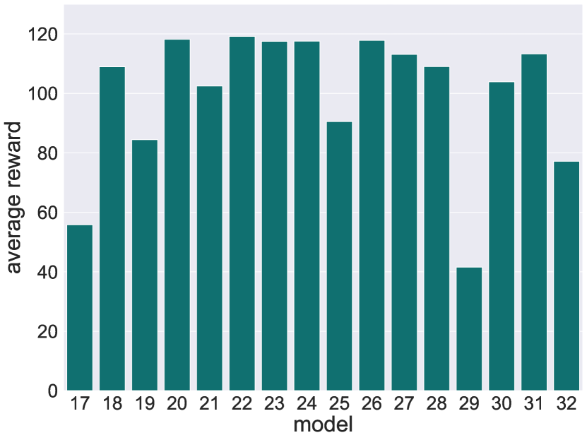
(c) OOD ($\sim\mathcal{TN}(\mu_{high},\sigma^{2}$))

Figure 29: Aurora: the models’ average rewards under different PDFs.
Top row: results for the models used in Experiment 8.
Bottom row: results for the models used in Experiment G.1.

(a) $\sim\mathcal{TN}(\mu_{low},\sigma^{2}$)

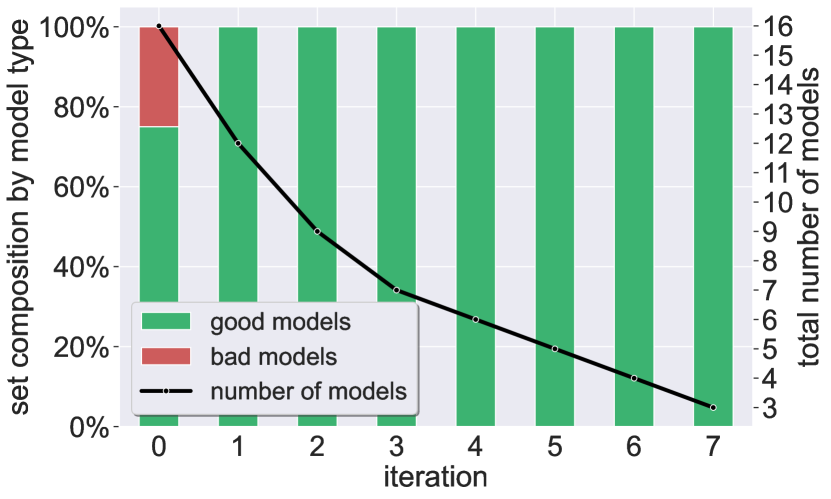
(b) $\sim\mathcal{TN}(\mu_{high},\sigma^{2}$)

Figure 32: Aurora: Additional PDFs: model selection results for OOD values; the models are the same as in Experiment G.1.

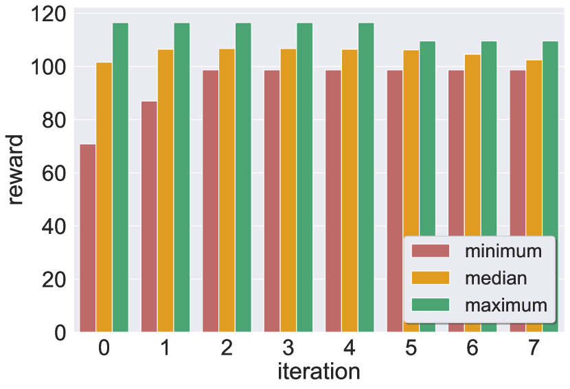
(a) $\sim\mathcal{TN}(\mu_{low},\sigma^{2}$)

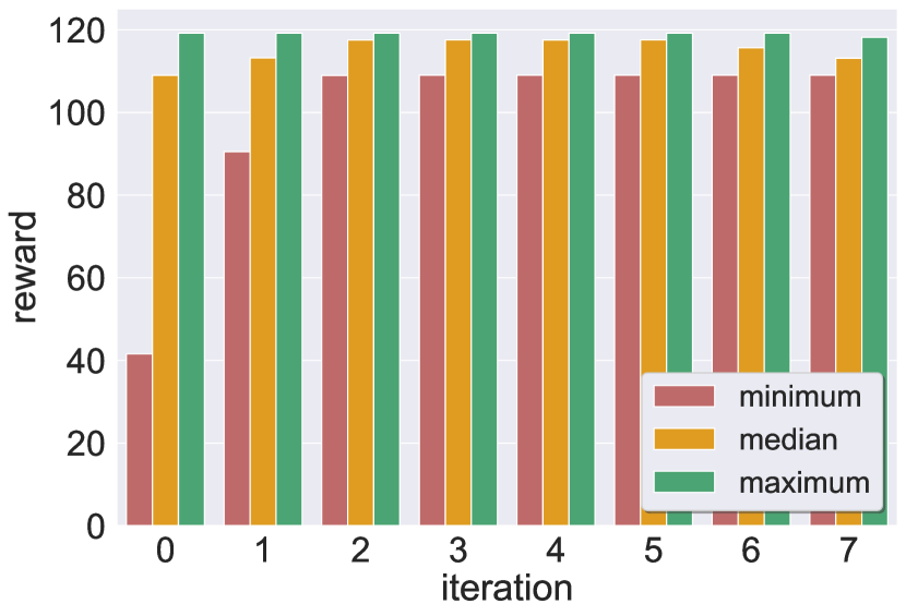
(b) $\sim\mathcal{TN}(\mu_{high},\sigma^{2}$)

Figure 33: Aurora: Additional PDFs: model selection results: rewards statistics per iteration; the models are the same as in Experiment G.1.

G.3 Additional Filtering Criteria: Experiment 8

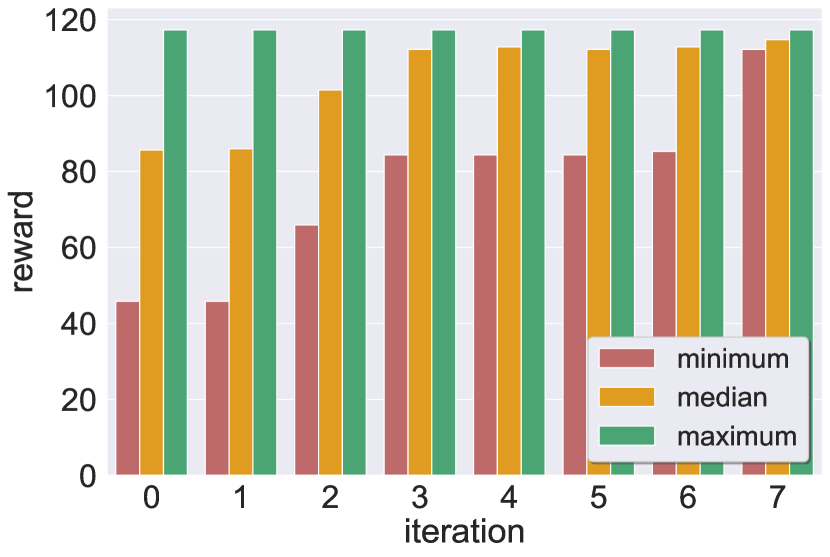
(a) Reward statistics of remaining models

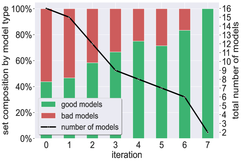
(b) Ratio between good/bad models

Figure 34: Aurora Experiment 8: results using the MAX filtering criterion. Our technique selected models {7,16}.

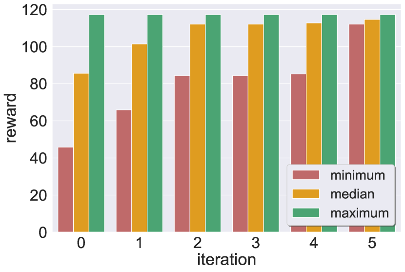
(a) Reward statistics of remaining models

(b) Ratio between good/bad models

Figure 35: Aurora Experiment 8: results using the COMBINED filtering criterion. Our technique selected models {7,16}.

G.4 Additional Filtering Criteria: Experiment G.1

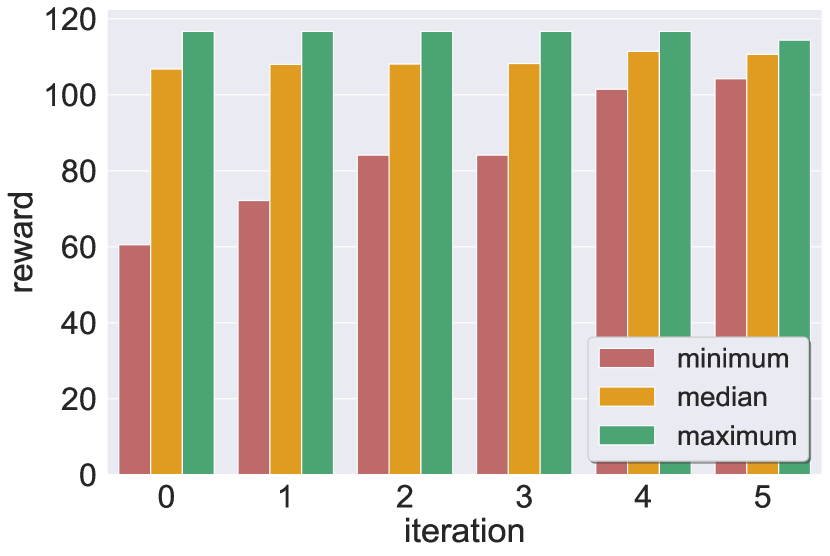
(a) Reward statistics of remaining models

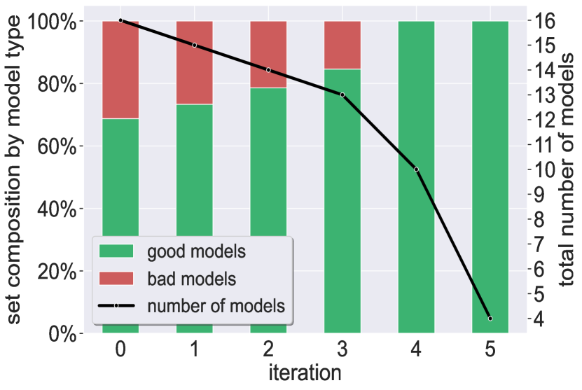
(b) Ratio between good/bad models

Figure 36: Aurora Experiment G.1: results using the MAX filtering criterion. Our technique selected models {20, 22, 27, 28}.

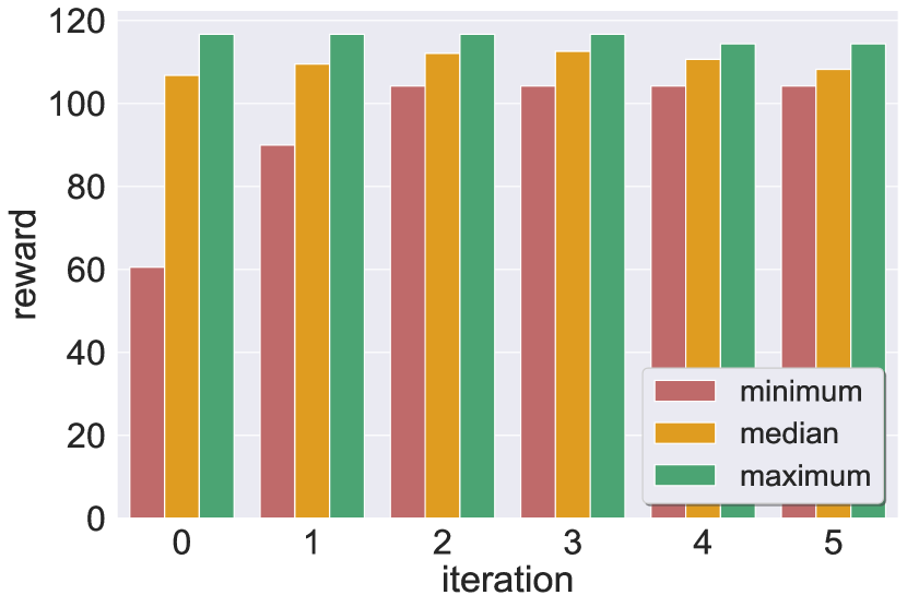
(a) Reward statistics of remaining models

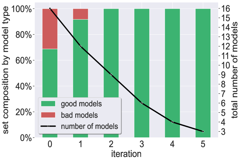
(b) Ratio between good/bad models

Figure 37: Aurora Experiment G.1: results using the COMBINED filtering criterion. Our technique selected models {20, 27, 28}.

G.5 Additional Filtering Criteria: Additional PDFs

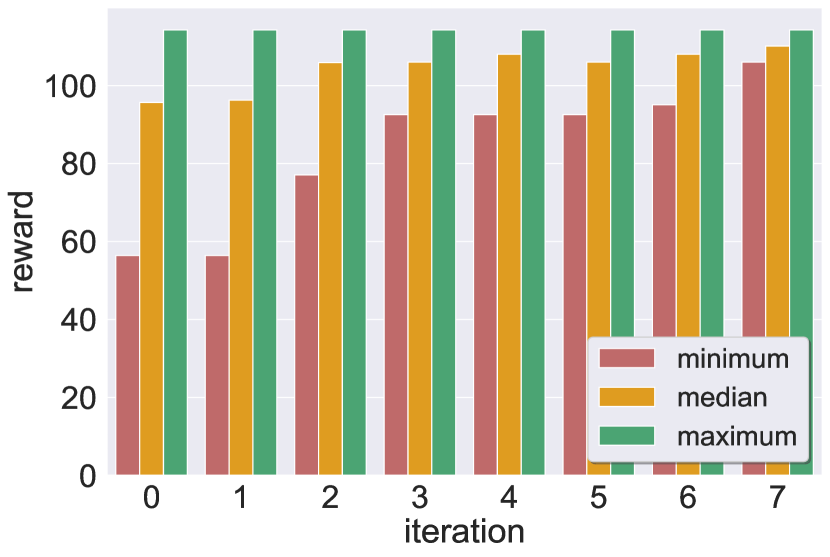
(a) Reward statistics of remaining models

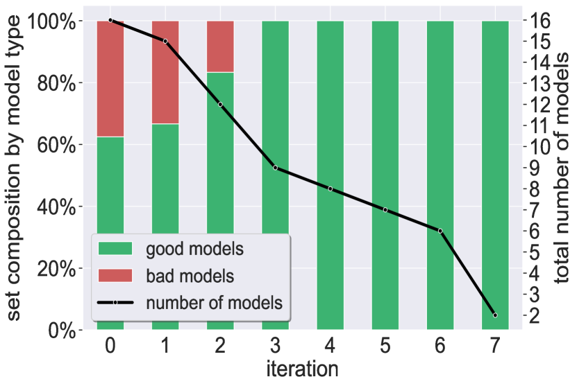
(b) Ratio between good/bad models

Figure 38: Aurora Experiment 8: PDF $\sim\mathcal{TN}(\mu_{low},\sigma^{2}$): results using the MAX filtering criterion.

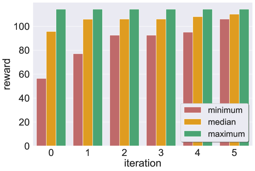
(a) Reward statistics of remaining models

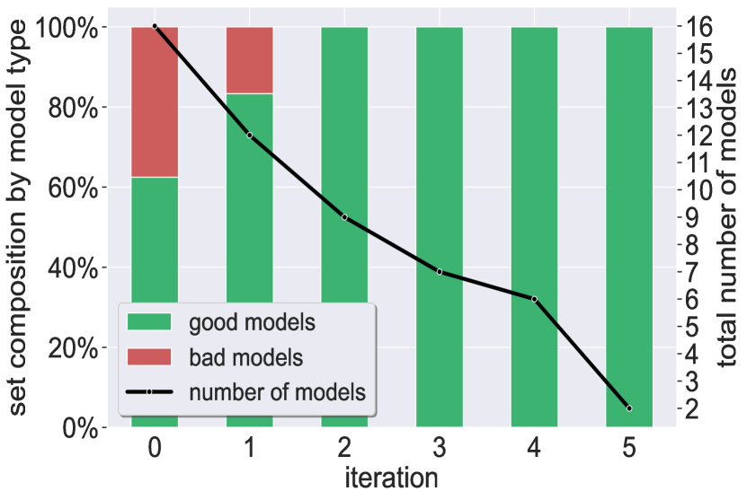
(b) Ratio between good/bad models

Figure 39: Aurora Experiment 8: PDF $\sim\mathcal{TN}(\mu_{low},\sigma^{2}$): results using the COMBINED filtering criterion.

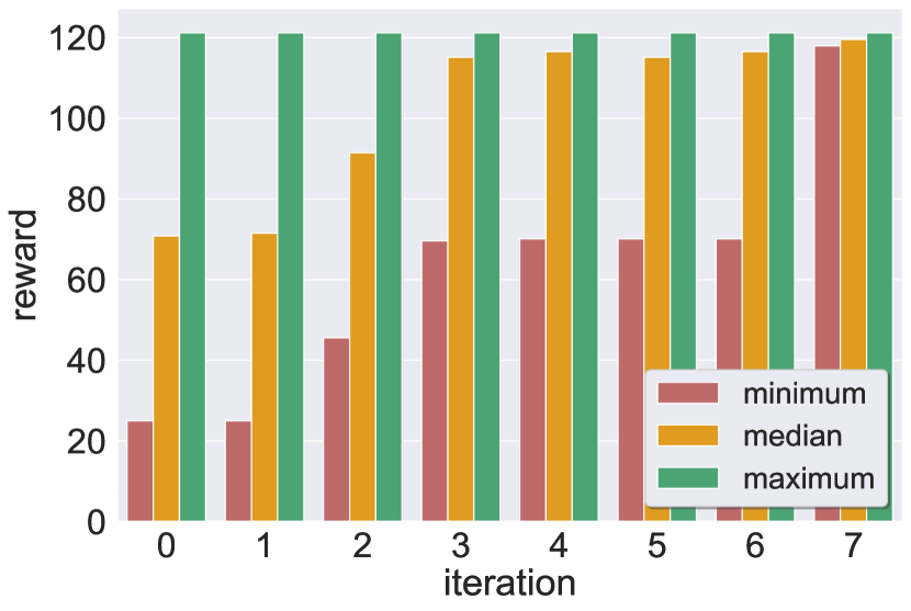
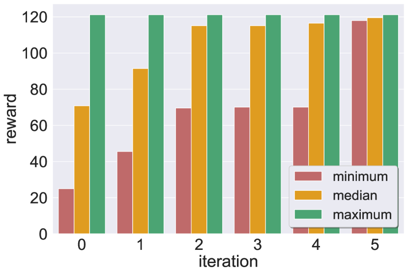
(a) Reward statistics of remaining models

(b) Ratio between good/bad models

Figure 40: Aurora Experiment 8: PDF $\sim\mathcal{TN}(\mu_{high},\sigma^{2}$): results using the MAX filtering criterion.

(a) Reward statistics of remaining models

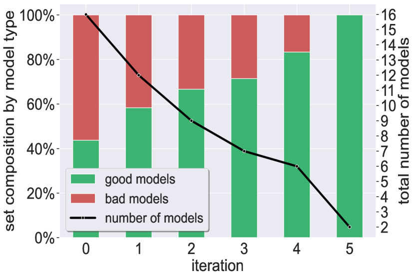
(b) Ratio between good/bad models

Figure 41: Aurora Experiment 8: PDF $\sim\mathcal{TN}(\mu_{high},\sigma^{2}$): results using the COMBINED filtering criterion.

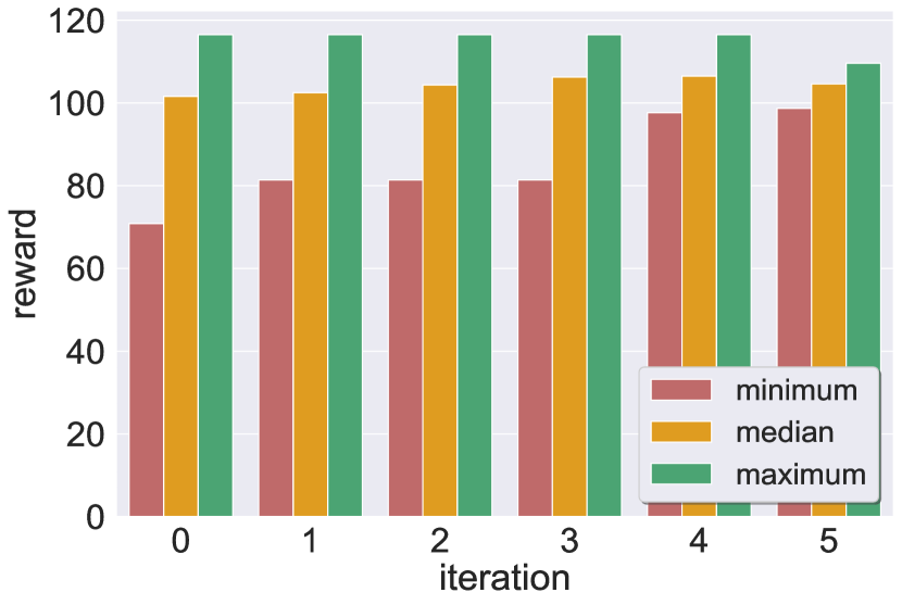
(a) Reward statistics of remaining models

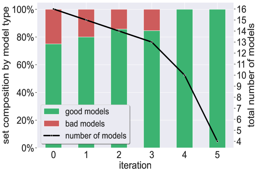
(b) Ratio between good/bad models

Figure 42: Aurora Experiment G.1:, PDF $\sim\mathcal{TN}(\mu_{low},\sigma^{2}$): results using the MAX filtering criterion.

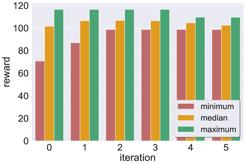
(a) Reward statistics of remaining models

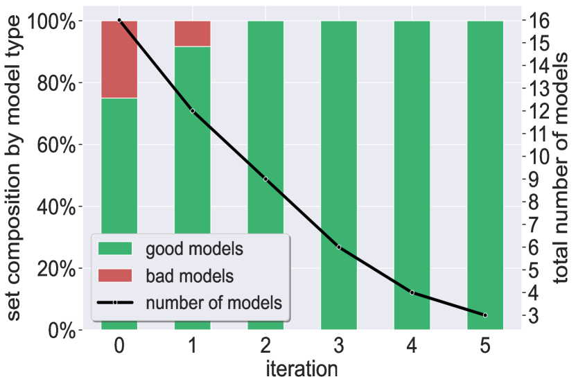
(b) Ratio between good/bad models

Figure 43: Aurora Experiment G.1: PDF $\sim\mathcal{TN}(\mu_{low},\sigma^{2}$): results using the COMBINED filtering criterion.

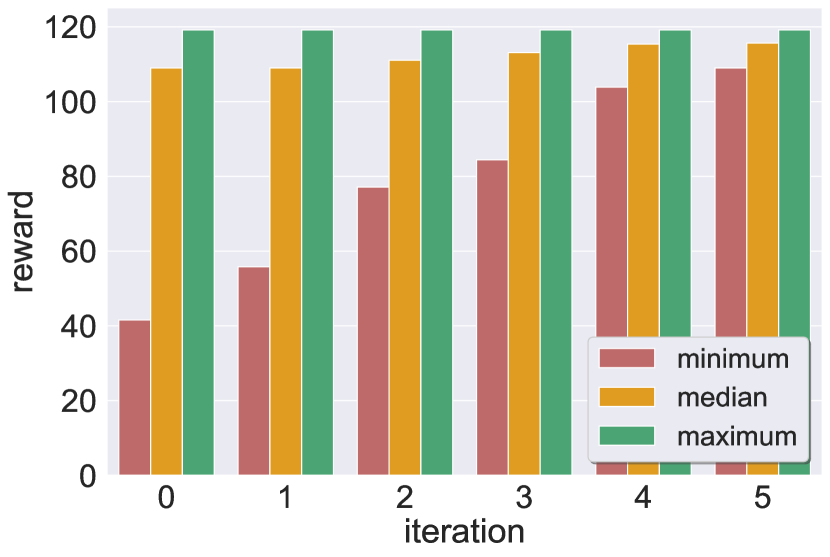
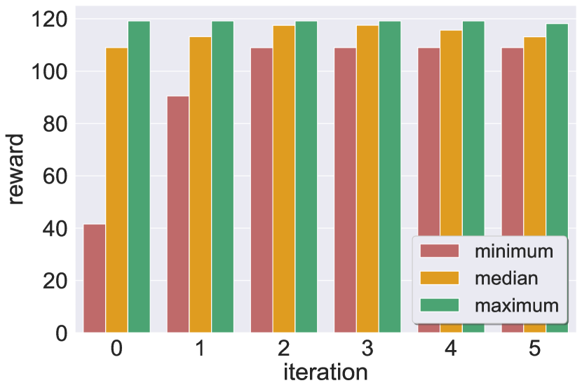
(a) Reward statistics of remaining models

(b) Ratio between good/bad models

Figure 44: Aurora Experiment G.1: PDF $\sim\mathcal{TN}(\mu_{high},\sigma^{2}$): results using the MAX filtering criterion.

(a) Reward statistics of remaining models

(b) Ratio between good/bad models

Figure 45: Aurora Experiment G.1: PDF $\sim\mathcal{TN}(\mu_{high},\sigma^{2}$): results using the COMBINED filtering criterion.

Appendix H Arithmetic DNNs: Supplementary Results

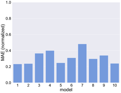
(a)

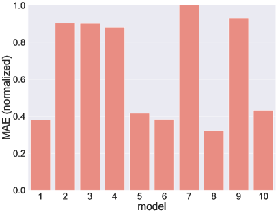
(b)

Figure 46: Arithmetic DNNs: the models’ maximal absolute error (MAE) when simulated on different distributions. The in-distribution results are normalized relative to the OOD range (i.e., multiplied by 100) and divided by the maximal error in the OOD case. The OOD results are normalized based on the maximal error in the OOD case (i.e., 210).

H.1 Additional Filtering Criteria

References

- \bibcommenthead
- Goodfellow et al. [2016] Goodfellow, I., Bengio, Y., Courville, A.: Deep Learning. MIT Press (2016)
- Simonyan and Zisserman [2014] Simonyan, K., Zisserman, A.: Very Deep Convolutional Networks for Large-Scale Image Recognition. Technical Report. http://arxiv.org/abs/1409.1556 (2014)
- Silver et al. [2016] Silver, D., Huang, A., Maddison, C., Guez, A., Sifre, L., Den Driessche, G., Schrittwieser, J., Antonoglou, I., Panneershelvam, V., Lanctot, M., Dieleman, S.: Mastering the Game of Go with Deep Neural Networks and Tree Search. Nature 529(7587), 484–489 (2016)
- AlQuraishi [2019] AlQuraishi, M.: AlphaFold at CASP13. Bioinformatics 35(22), 4862–4865 (2019)
- Collobert et al. [2011] Collobert, R., Weston, J., Bottou, L., Karlen, M., Kavukcuoglu, K., Kuksa, P.: Natural Language Processing (Almost) from Scratch. Journal of Machine Learning Research (JMLR) 12, 2493–2537 (2011)
- Krizhevsky et al. [2012] Krizhevsky, A., Sutskever, I., Hinton, G.: Imagenet Classification with Deep Convolutional Neural Networks. In: Proc. 26th Conf. on Neural Information Processing Systems (NeurIPS), pp. 1097–1105 (2012)
- Bojarski et al. [2016] Bojarski, M., Del Testa, D., Dworakowski, D., Firner, B., Flepp, B., Goyal, P., Jackel, L., Monfort, M., Muller, U., Zhang, J., Zhang, X., Zhao, J., Zieba, K.: End to End Learning for Self-Driving Cars. Technical Report. http://arxiv.org/abs/1604.07316 (2016)
- Julian et al. [2016] Julian, K., Lopez, J., Brush, J., Owen, M., Kochenderfer, M.: Policy Compression for Aircraft Collision Avoidance Systems. In: Proc. 35th Digital Avionics Systems Conf. (DASC), pp. 1–10 (2016)
- Li [2017] Li, Y.: Deep Reinforcement Learning: An Overview. Technical Report. http://arxiv.org/abs/1701.07274 (2017)
- Mnih et al. [2013] Mnih, V., Kavukcuoglu, K., Silver, D., Graves, A., Antonoglou, I., Wierstra, D., Riedmiller, M.: Playing Atari with Deep Reinforcement Learning. Technical Report. https://arxiv.org/abs/1312.5602 (2013)
- Zhang et al. [2019] Zhang, J., Liu, Y., Zhou, K., Li, G., Xiao, Z., Cheng, B., Xing, J., Wang, Y., Cheng, T., Liu, L., et al.: An End-to-End Automatic Cloud Database Tuning System Using Deep Reinforcement Learning. In: Proc. of the 2019 Int. Conf. on Management of Data (SIGMOD), pp. 415–432 (2019)
- Mammadli et al. [2020] Mammadli, R., Jannesari, A., Wolf, F.: Static Neural Compiler Optimization via Deep Reinforcement Learning. In: Proc. 6th IEEE/ACM Workshop on the LLVM Compiler Infrastructure in HPC (LLVM-HPC) and Workshop on Hierarchical Parallelism for Exascale Computing (HiPar), pp. 1–11 (2020)
- Li et al. [2018] Li, W., Zhou, F., Chowdhury, K.R., Meleis, W.: QTCP: Adaptive Congestion Control with Reinforcement Learning. IEEE Transactions on Network Science and Engineering 6(3), 445–458 (2018)
- Jay et al. [2019] Jay, N., Rotman, N., Godfrey, B., Schapira, M., Tamar, A.: A Deep Reinforcement Learning Perspective on Internet Congestion Control. In: Proc. 36th Int. Conf. on Machine Learning (ICML), pp. 3050–3059 (2019)
- Valadarsky et al. [2017] Valadarsky, A., Schapira, M., Shahaf, D., Tamar, A.: Learning to Route with Deep RL. In: NeurIPS Deep Reinforcement Learning Symposium (2017)
- Chen et al. [2017] Chen, W., Xu, Y., Wu, X.: Deep Reinforcement Learning for Multi-Resource Multi-Machine Job Scheduling. Technical Report. http://arxiv.org/abs/1711.07440 (2017)
- Mao et al. [2016] Mao, H., Alizadeh, M., Menache, I., Kandula, S.: Resource Management with Deep Reinforcement Learning. In: Proc. 15th ACM Workshop on Hot Topics in Networks (HotNets), pp. 50–56 (2016)
- Lekharu et al. [2020] Lekharu, A., Moulii, K.Y., Sur, A., Sarkar, A.: Deep Learning Based Prediction Model for Adaptive Video Streaming. In: Proc. 12th Int. Conf. on Communication Systems & Networks (COMSNETS), pp. 152–159 (2020). IEEE
- Mao et al. [2017] Mao, H., Netravali, R., Alizadeh, M.: Neural Adaptive Video Streaming with Pensieve. In: Proc. Conf. of the ACM Special Interest Group on Data Communication on the Applications, Technologies, Architectures, and Protocols for Computer Communication (SIGCOMM), pp. 197–210 (2017)
- Tolstoy [1877] Tolstoy, L.: Anna Karenina. The Russian Messenger (1877)
- Lukina et al. [2021] Lukina, A., Schilling, C., Henzinger, T.: Into the Unknown: Active Monitoring of Neural Networks. In: Proc. 21st Int. Conf. on Runtime Verification (RV), pp. 42–61 (2021)
- Alamdari et al. [2020] Alamdari, P., Avni, G., Henzinger, T., Lukina, A.: Formal Methods with a Touch of Magic. In: Proc. 20th Int. Conf. on Formal Methods in Computer-Aided Design (FMCAD), pp. 138–147 (2020)
- Avni et al. [2019] Avni, G., Bloem, R., Chatterjee, K., Henzinger, T., Könighofer, B., Pranger, S.: Run-Time Optimization for Learned Controllers through Quantitative Games. In: Proc. 31st Int. Conf. on Computer Aided Verification (CAV), pp. 630–649 (2019)
- Baluta et al. [2019] Baluta, T., Shen, S., Shinde, S., Meel, K., Saxena, P.: Quantitative Verification of Neural Networks and its Security Applications. In: Proc. ACM SIGSAC Conf. on Computer and Communications Security (CCS), pp. 1249–1264 (2019)
- Prabhakar and Afzal [2020] Prabhakar, P., Afzal, Z.: Abstraction Based Output Range Analysis for Neural Networks. Technical Report. https://arxiv.org/abs/2007.09527 (2020)
- Anderson et al. [2019] Anderson, G., Pailoor, S., Dillig, I., Chaudhuri, S.: Optimization and Abstraction: a Synergistic Approach for Analyzing Neural Network Robustness. In: Proc. 40th ACM SIGPLAN Conf. on Programming Languages Design and Implementations (PLDI), pp. 731–744 (2019)
- Singh et al. [2019] Singh, G., Gehr, T., Puschel, M., Vechev, M.: An Abstract Domain for Certifying Neural Networks. In: Proc. 46th ACM SIGPLAN Symposium on Principles of Programming Languages (POPL) (2019)
- Xiang et al. [2018] Xiang, W., Tran, H., Johnson, T.: Output Reachable Set Estimation and Verification for Multi-Layer Neural Networks. IEEE Transactions on Neural Networks and Learning Systems (TNNLS) (2018)
- Ehlers [2017] Ehlers, R.: Formal Verification of Piece-Wise Linear Feed-Forward Neural Networks. In: Proc. 15th Int. Symp. on Automated Technology for Verification and Analysis (ATVA), pp. 269–286 (2017)
- Gehr et al. [2018] Gehr, T., Mirman, M., Drachsler-Cohen, D., Tsankov, E., Chaudhuri, S., Vechev, M.: AI2: Safety and Robustness Certification of Neural Networks with Abstract Interpretation. In: Proc. 39th IEEE Symposium on Security and Privacy (S&P) (2018)
- Lyu et al. [2020] Lyu, Z., Ko, C.Y., Kong, Z., Wong, N., Lin, D., Daniel, L.: Fastened Crown: Tightened Neural Network Robustness Certificates. In: Proc. 34th AAAI Conf. on Artificial Intelligence (AAAI), pp. 5037–5044 (2020)
- Gopinath et al. [2018] Gopinath, D., Katz, G., Pǎsǎreanu, C., Barrett, C.: DeepSafe: A Data-driven Approach for Assessing Robustness of Neural Networks. In: Proc. 16th. Int. Symposium on Automated Technology for Verification and Analysis (ATVA), pp. 3–19 (2018)
- Trask et al. [2018] Trask, A., Hill, F., Reed, S., Rae, J., C., D., Blunsom, P.: Neural Arithmetic Logic Units. In: Proc. 32nd Conf. on Neural Information Processing Systems (NeurIPS) (2018)
- Madsen and Johansen [2020] Madsen, A., Johansen, A.: Neural Arithmetic Units. In: Proc. 8th Int. Conf. on Learning Representations (ICLR) (2020)
- Amir et al. [2024] Amir, G., Maayan, O., Zelazny, T., Katz, G., Schapira, M.: Verifying the Generalization of Deep Learning to Out-of-Distribution Domains: Artifact. https://zenodo.org/records/10448320 (2024)
- Amir et al. [2023] Amir, G., Maayan, O., Zelazny, T., Katz, G., Schapira, M.: Verifying Generalization in Deep Learning. In: Proc. 35th Int. Conf. on Computer Aided Verification (CAV), pp. 438–455 (2023)
- Sutton and Barto [2018] Sutton, R., Barto, A.: Reinforcement Learning: An Introduction. MIT Press (2018)
- Zhang et al. [2020] Zhang, J., Kim, J., O’Donoghue, B., Boyd, S.: Sample Efficient Reinforcement Learning with REINFORCE. Technical Report. https://arxiv.org/abs/2010.11364 (2020)
- Schulman et al. [2017] Schulman, J., Wolski, F., Dhariwal, P., Radford, A., Klimov, O.: Proximal Policy Optimization Algorithms. Technical Report. http://arxiv.org/abs/1707.06347 (2017)
- van Hasselt et al. [2016] Hasselt, H., Guez, A., Silver, D.: Deep Reinforcement Learning with Double Q-Learning. In: Proc. 30th AAAI Conf. on Artificial Intelligence (AAAI) (2016)
- Sutton et al. [1999] Sutton, R., McAllester, D., Singh, S., Mansour, Y.: Policy Gradient Methods for Reinforcement Learning with Function Approximation. In: Proc. 12th Conf. on Neural Information Processing Systems (NeurIPS) (1999)
- Haarnoja et al. [2018] Haarnoja, T., Zhou, A., Abbeel, P., Levine, S.: Soft Actor-Critic: Off-Policy Maximum Entropy Deep Reinforcement Learning with a Stochastic Actor. In: Int. Conf. on Machine Learning, pp. 1861–1870 (2018). PMLR
- Katz et al. [2017] Katz, G., Barrett, C., Dill, D., Julian, K., Kochenderfer, M.: Reluplex: An Efficient SMT Solver for Verifying Deep Neural Networks. In: Proc. 29th Int. Conf. on Computer Aided Verification (CAV), pp. 97–117 (2017)
- Albarghouthi [2021] Albarghouthi, A.: Introduction to Neural Network Verification. verifieddeeplearning.com (2021)
- Wang et al. [2018] Wang, S., Pei, K., Whitehouse, J., Yang, J., Jana, S.: Formal Security Analysis of Neural Networks using Symbolic Intervals. In: Proc. 27th USENIX Security Symposium, pp. 1599–1614 (2018)
- Huang et al. [2017] Huang, X., Kwiatkowska, M., Wang, S., Wu, M.: Safety Verification of Deep Neural Networks. In: Proc. 29th Int. Conf. on Computer Aided Verification (CAV), pp. 3–29 (2017)
- Barto et al. [1983] Barto, A., Sutton, R., Anderson, C.: Neuronlike Adaptive Elements that Can Solve Difficult Learning Control Problems. In: Proc. of IEEE Systems Man and Cybernetics Conference (SMC), pp. 834–846 (1983)
- Moore [1990] Moore, A.: Efficient Memory-based Learning for Robot Control. University of Cambridge (1990)
- Katz et al. [2019] Katz, G., Huang, D., Ibeling, D., Julian, K., Lazarus, C., Lim, R., Shah, P., Thakoor, S., Wu, H., Zeljić, A., Dill, D., Kochenderfer, M., Barrett, C.: The Marabou Framework for Verification and Analysis of Deep Neural Networks. In: Proc. 31st Int. Conf. on Computer Aided Verification (CAV), pp. 443–452 (2019)
- Wu et al. [2024] Wu, H., Isac, O., Zeljić, A., Tagomori, T., Daggitt, M., Kokke, W., Refaeli, I., Amir, G., Julian, K., Bassan, S., et al.: Marabou 2.0: A Versatile Formal Analyzer of Neural Networks. In: Proc. 36th Int. Conf. on Computer Aided Verification (CAV) (2024)
- Geva and Sitte [1993] Geva, S., Sitte, J.: A Cartpole Experiment Benchmark for Trainable Controllers. IEEE Control Systems Magazine 13(5), 40–51 (1993)
- Riedmiller [2005] Riedmiller, M.: Neural Fitted Q Iteration — First Experiences with a Data Efficient Neural Reinforcement Learning Method. In: Proc. 16th European Conf. on Machine Learning (ECML), pp. 317–328 (2005)
- Low et al. [2002] Low, S., Paganini, F., Doyle, J.: Internet Congestion Control. IEEE Control Systems Magazine 22(1), 28–43 (2002)
- Nagle [1984] Nagle, J.: Congestion Control in IP/TCP Internetworks. ACM SIGCOMM Computer Communication Review 14(4), 11–17 (1984)
- Eliyahu et al. [2021] Eliyahu, T., Kazak, Y., Katz, G., Schapira, M.: Verifying Learning-Augmented Systems. In: Proc. Conf. of the ACM Special Interest Group on Data Communication on the Applications, Technologies, Architectures, and Protocols for Computer Communication (SIGCOMM), pp. 305–318 (2021)
- Amir et al. [2021] Amir, G., Schapira, M., Katz, G.: Towards Scalable Verification of Deep Reinforcement Learning. In: Proc. 21st Int. Conf. on Formal Methods in Computer-Aided Design (FMCAD), pp. 193–203 (2021)
- Kingma and Ba [2015] Kingma, D., Ba, J.: Adam: A Method for Stochastic Optimization . In: Proc. 3rd Int. Conf. on Learning Representations (ICLR) (2015)
- Lakshminarayanan et al. [2017] Lakshminarayanan, B., Pritzel, A., Blundell, C.: Simple and Scalable Predictive Uncertainty Estimation Using Deep Ensembles. In: Proc. 30th Conf. on Neural Information Processing Systems (NeurIPS) (2017)
- Katz et al. [2021] Katz, G., Barrett, C., Dill, D., Julian, K., Kochenderfer, M.: Reluplex: A Calculus for Reasoning about Deep Neural Networks. Formal Methods in System Design (FMSD) (2021)
- Ruder [2016] Ruder, S.: An Overview of Gradient Descent Optimization Algorithms. Technical Report. https://arxiv.org/abs/1609.04747 (2016)
- Ma et al. [2020] Ma, J., Ding, S., Mei, Q.: Towards More Practical Adversarial Attacks on Graph Neural Networks. In: Proc. 34th Conf. on Neural Information Processing Systems (NeurIPS) (2020)
- Kurakin et al. [2016] Kurakin, A., Goodfellow, I., Bengio, S.: Adversarial Examples in the Physical World. Technical Report. http://arxiv.org/abs/1607.02533 (2016)
- Wu et al. [2022] Wu, H., Zeljić, A., Katz, K., Barrett, C.: Efficient Neural Network Analysis with Sum-of-Infeasibilities. In: Proc. 28th Int. Conf. on Tools and Algorithms for the Construction and Analysis of Systems (TACAS), pp. 143–163 (2022)
- Amir et al. [2022] Amir, G., Zelazny, T., Katz, G., Schapira, M.: Verification-Aided Deep Ensemble Selection. In: Proc. 22nd Int. Conf. on Formal Methods in Computer-Aided Design (FMCAD), pp. 27–37 (2022)
- Huang et al. [2017] Huang, S., Papernot, N., Goodfellow, I., Duan, Y., Abbeel, P.: Adversarial Attacks on Neural Network Policies. Technical Report. https://arxiv.org/abs/1702.02284 (2017)
- Madry et al. [2017] Madry, A., Makelov, A., Schmidt, L., Tsipras, D., Vladu, A.: Towards Deep Learning Models Resistant to Adversarial Attacks. Technical Report. http://arxiv.org/abs/1706.06083 (2017)
- Rockafellar [1993] Rockafellar, T.: Lagrange Multipliers and Optimality. SIAM Review 35(2), 183–238 (1993)
- Ovadia et al. [2019] Ovadia, Y., Fertig, E., Ren, J., Nado, Z., Sculley, D., Nowozin, S., Dillon, J., Lakshminarayanan, B., Snoek, J.: Can You Trust Your Model’s Uncertainty? Evaluating Predictive Uncertainty Under Dataset Shift. In: Proc. 33rd Conf. on Neural Information Processing Systems (NeurIPS), pp. 14003–14014 (2019)
- Abdar et al. [2021] Abdar, M., Pourpanah, F., Hussain, S., Rezazadegan, D., Liu, L., Ghavamzadeh, M., Fieguth, P., Cao, X., Khosravi, A., Acharya, U., Makarenkov, V., Nahavandi, S.: A Review of Uncertainty Quantification in Deep Learning: Techniques, Applications and Challenges. Information Fusion 76, 243–297 (2021)
- Krogh and Vedelsby [1994] Krogh, A., Vedelsby, J.: Neural Network Ensembles, Cross Validation, and Active Learning. In: Proc. 7th Conf. on Neural Information Processing Systems (NeurIPS), pp. 231–238 (1994)
- Dietterich [2020] Dietterich, T.: Ensemble Methods in Machine Learning. In: Proc. 1st Int. Workshop on Multiple Classifier Systems (MCS), pp. 1–15 (2020)
- Ganaie et al. [2022] Ganaie, M., Hu, M., Malik, A., Tanveer, M., Suganthan, P.: Ensemble Deep Learning: A Review. Engineering Applications of Artificial Intelligence 115, 105151 (2022)
- Loquercio et al. [2020] Loquercio, A., Segu, M., Scaramuzza, D.: A General Framework for Uncertainty Estimation in Deep Learning. In: Proc. Int. Conf. on Robotics and Automation (ICRA), pp. 3153–3160 (2020)
- Szegedy et al. [2013] Szegedy, C., Zaremba, W., Sutskever, I., Bruna, J., Erhan, D., Goodfellow, I., Fergus, R.: Intriguing Properties of Neural Networks. Technical Report. http://arxiv.org/abs/1312.6199 (2013)
- Goodfellow et al. [2014] Goodfellow, I., Shlens, J., Szegedy, C.: Explaining and Harnessing Adversarial Examples. Technical Report. http://arxiv.org/abs/1412.6572 (2014)
- Papernot et al. [2016] Papernot, N., McDaniel, P., Jha, S., Fredrikson, M., Celik, Z., Swami, A.: The Limitations of Deep Learning in Adversarial Settings. In: IEEE European Symposium on Security and Privacy (EuroS&P), pp. 372–387 (2016)
- Papernot et al. [2017] Papernot, N., McDaniel, P., Goodfellow, I., Jha, S., Celik, Z., Swami, A.: Practical Black-Box Attacks against Machine Learning. In: Proc. ACM on Asia Conf. on Computer and Communications Security (CCS, pp. 506–519 (2017)
- Moosavi-Dezfooli et al. [2016] Moosavi-Dezfooli, M.D., Fawzi, A., Frossard, P.: DeepFool: A Simple and Accurate Method to Fool Deep Neural Networks. In: Proc. IEEE Conf. on Computer Vision and Pattern Recognition (CVPR) (2016)
- Fawaz et al. [2019] Fawaz, H., Forestier, G., Weber, J., Idoumghar, L., Muller, P.-A.: Adversarial Attacks on Deep Neural Networks for Time Series Classification. In: Proc. Int. Joint Conf. on Neural Networks (IJCNN), pp. 1–8 (2019)
- Zügner et al. [2018] Zügner, D., Akbarnejad, A., Günnemann, S.: Adversarial Attacks on Neural Networks for Graph Data. In: Proc. 24th ACM SIGKDD Int. Conf. on Knowledge Discovery & Data Mining (KDD), pp. 2847–2856 (2018)
- Cisse et al. [2017] Cisse, M., Bojanowski, P., Grave, E., Dauphin, Y., Usunier, N.: Parseval Networks: Improving Robustness to Adversarial Examples. In: Proc. 34th Int. Conf. on Machine Learning (ICML), pp. 854–863 (2017)
- Cohen et al. [2019] Cohen, J., Rosenfeld, E., Kolter, Z.: Certified Adversarial Robustness via Randomized Smoothing. In: Proc. 36th Int. Conf. on Machine Learning (ICML), pp. 1310–1320 (2019)
- Qin et al. [2019] Qin, C., Martens, J., Gowal, S., Krishnan, D., Dvijotham, K., Fawzi, A., De, S., Stanforth, R., Kohli, P.: Adversarial Robustness through Local Linearization. Technical Report. http://arxiv.org/abs/1907.02610 (2019)
- Wong et al. [2020] Wong, E., Rice, L., Kolter, Z.: Fast is Better than Free: Revisiting Adversarial Training. Technical Report. http://arxiv.org/abs/2001.03994 (2020)
- Shafahi et al. [2019] Shafahi, A., Najibi, M., Ghiasi, A., Xu, Z., Dickerson, J., Studer, C., Davis, L., Taylor, G., Goldstein, T.: Adversarial Training for Free! Technical Report. http://arxiv.org/abs/1904.12843 (2019)
- Ganin et al. [2016] Ganin, Y., Ustinova, E., Ajakan, H., Germain, P., Larochelle, H., Laviolette, F., Marchand, M., Lempitsky, V.: Domain-Adversarial Training of Neural Networks. Journal of Machine Learning Research (JMLR) 17(1), 2096–2030 (2016)
- Han et al. [2018] Han, B., Yao, Q., Yu, X., Niu, G., Xu, M., Hu, W., Tsang, I., Sugiyama, M.: Co-teaching: Robust Training of Deep Neural Networks with Extremely Noisy Labels. Technical Report. http://arxiv.org/abs/1804.06872 (2018)
- Yu et al. [2019] Yu, X., Han, B., Yao, J., Niu, G., Tsang, I., Sugiyama, M.: How does Disagreement Help Generalization against Label Corruption? In: Proc. 36th Int. Conf. on Machine Learning (ICML), pp. 7164–7173 (2019)
- Liu et al. [2019] Liu, H., Long, M., Wang, J., Jordan, M.: Transferable Adversarial Training: A General Approach to Adapting Deep Classifiers. In: Proc. 36th Int. Conf. on Machine Learning (ICML), pp. 4013–4022 (2019)
- Shafahi et al. [2019] Shafahi, A., Saadatpanah, P., Zhu, C., Ghiasi, A., Studer, C., Jacobs, D., Goldstein, T.: Adversarially Robust Transfer Learning. Technical Report. http://arxiv.org/abs/1905.08232 (2019)
- Tjeng et al. [2019] Tjeng, V., Xiao, K., Tedrake, R.: Evaluating Robustness of Neural Networks with Mixed Integer Programming. In: Proc. 7th Int. Conf. on Learning Representations (ICLR) (2019)
- Könighofer et al. [2020] Könighofer, B., Lorber, F., Jansen, N., Bloem, R.: Shield Synthesis for Reinforcement Learning. In: Proc. Int. Symposium on Leveraging Applications of Formal Methods, Verification and Validation (ISoLA), pp. 290–306 (2020)
- Wu et al. [2020] Wu, H., Ozdemir, A., Zeljić, A., Irfan, A., Julian, K., Gopinath, D., Fouladi, S., Katz, G., Păsăreanu, C., Barrett, C.: Parallelization Techniques for Verifying Neural Networks. In: Proc. 20th Int. Conf. on Formal Methods in Computer-Aided Design (FMCAD), pp. 128–137 (2020)
- Seshia et al. [2018] Seshia, S., Desai, A., Dreossi, T., Fremont, D., Ghosh, S., Kim, E., Shivakumar, S., Vazquez-Chanlatte, M., Yue, X.: Formal Specification for Deep Neural Networks. In: Proc. 16th Int. Symposium on Automated Technology for Verification and Analysis (ATVA), pp. 20–34 (2018)
- Polgreen et al. [2020] Polgreen, E., Abboud, R., Kroening, D.: Counterexample Guided Neural Synthesis. Technical Report. https://arxiv.org/abs/2001.09245 (2020)
- Okudono et al. [2020] Okudono, T., Waga, M., Sekiyama, T., Hasuo, I.: Weighted Automata Extraction from Recurrent Neural Networks via Regression on State Spaces. In: Proc. 34th AAAI Conf. on Artificial Intelligence (AAAI), pp. 5037–5044 (2020)
- Goubault et al. [2021] Goubault, E., Palumby, S., Putot, S., Rustenholz, L., Sankaranarayanan, S.: Static Analysis of ReLU Neural Networks with Tropical Polyhedra. In: Proc. 28th Int. Symposium on Static Analysis (SAS), pp. 166–190 (2021)
- Vasić et al. [2022] Vasić, M., Petrović, A., Wang, K., Nikolić, M., Singh, R., Khurshid, S.: MoËT: Mixture of Expert Trees and its Application to Verifiable Reinforcement Learning. Neural Networks 151, 34–47 (2022)
- Bacci et al. [2021] Bacci, E., Giacobbe, M., Parker, D.: Verifying Reinforcement Learning up to Infinity. In: Proc. 30th Int. Joint Conf. on Artificial Intelligence (IJCAI) (2021)
- Dutta et al. [2019] Dutta, S., Chen, X., Sankaranarayanan, S.: Reachability Analysis for Neural Feedback Systems using Regressive Polynomial Rule Inference. In: Proc. 22nd ACM Int. Conf. on Hybrid Systems: Computation and Control (HSCC), pp. 157–168 (2019)
- Dutta et al. [2018] Dutta, S., Jha, S., Sankaranarayanan, S., Tiwari, A.: Learning and Verification of Feedback Control Systems using Feedforward Neural Networks. IFAC-PapersOnLine 51(16), 151–156 (2018)
- Sun et al. [2019] Sun, X., Khedr, H., Shoukry, Y.: Formal Verification of Neural Network Controlled Autonomous Systems. In: Proc. 22nd ACM Int. Conf. on Hybrid Systems: Computation and Control (HSCC) (2019)
- Fulton and Platzer [2018] Fulton, N., Platzer, A.: Safe Reinforcement Learning via Formal Methods: Toward Safe Control through Proof and Learning. In: Proc. 32nd AAAI Conf. on Artificial Intelligence (AAAI) (2018)
- Corsi et al. [2021] Corsi, D., Marchesini, E., Farinelli, A.: Formal Verification of Neural Networks for Safety-Critical Tasks in Deep Reinforcement Learning. In: Proc. 37th Conf. on Uncertainty in Artificial Intelligence (UAI), pp. 333–343 (2021)
- Geng et al. [2022] Geng, C., Le, N., Xu, X., Wang, Z., Gurfinkel, A., Si, X.: Toward Reliable Neural Specifications. Technical Report. https://arxiv.org/abs/2210.16114 (2022)
- Ruan et al. [2018] Ruan, W., Huang, X., Kwiatkowska, M.: Reachability Analysis of Deep Neural Networks with Provable Guarantees. In: Proc. 27th Int. Joint Conf. on Artificial Intelligence (IJCAI) (2018)
- Isac et al. [2022] Isac, O., Barrett, C., Zhang, M., Katz, G.: Neural Network Verification with Proof Production. In: Proc. 22nd Int. Conf. on Formal Methods in Computer-Aided Design (FMCAD), pp. 38–48 (2022)
- Urban et al. [2020] Urban, C., Christakis, M., Wüstholz, V., Zhang, F.: Perfectly Parallel Fairness Certification of Neural Networks. In: Proc. ACM Int. Conf. on Object Oriented Programming Systems Languages and Applications (OOPSLA), pp. 1–30 (2020)
- Sotoudeh and Thakur [2019] Sotoudeh, M., Thakur, A.: Correcting Deep Neural Networks with Small, Generalizing Patches. In: Workshop on Safety and Robustness in Decision Making (2019)
- Yang et al. [2022] Yang, X., Yamaguchi, T., Tran, H., Hoxha, B., Johnson, T., Prokhorov, D.: Neural Network Repair with Reachability Analysis. In: Proc. 20th Int. Conf. on Formal Modeling and Analysis of Timed Systems (FORMATS), pp. 221–236 (2022)
- Goldberger et al. [2020] Goldberger, B., Adi, Y., Keshet, J., Katz, G.: Minimal Modifications of Deep Neural Networks using Verification. In: Proc. 23rd Int. Conf. on Logic for Programming, Artificial Intelligence and Reasoning (LPAR), pp. 260–278 (2020)
- Dong et al. [2020] Dong, G., Sun, J., Wang, J., Wang, X., Dai, T.: Towards Repairing Neural Networks Correctly. Technical Report. http://arxiv.org/abs/2012.01872 (2020)
- Usman et al. [2021] Usman, M., Gopinath, D., Sun, Y., Noller, Y., Pǎsǎreanu, C.: NNrepair: Constraint-based Repair of Neural Network Classifiers. Technical Report. http://arxiv.org/abs/2103.12535 (2021)
- Zhang et al. [2020] Zhang, H., Shinn, M., Gupta, A., Gurfinkel, A., Le, N., Narodytska, N.: Verification of Recurrent Neural Networks for Cognitive Tasks via Reachability Analysis. In: Proc. 24th European Conf. on Artificial Intelligence (ECAI), pp. 1690–1697 (2020)
- Jacoby et al. [2020] Jacoby, Y., Barrett, C., Katz, G.: Verifying Recurrent Neural Networks using Invariant Inference. In: Proc. 18th Int. Symposium on Automated Technology for Verification and Analysis (ATVA), pp. 57–74 (2020)
- Corsi et al. [2024] Corsi, D., Amir, G., Katz, G., Farinelli, A.: Analyzing Adversarial Inputs in Deep Reinforcement Learning. Technical Report. https://arxiv.org/abs/2402.05284 (2024)
- Mandal et al. [2024] Mandal, U., Amir, G., Wu, H., Daukantas, I., Newell, F., Ravaioli, U., Meng, B., Durling, M., Ganai, M., Shim, T., Katz, G., Barrett, C.: Formally Verifying Deep Reinforcement Learning Controllers with Lyapunov Barrier Certificates. Technical Report. https://arxiv.org/abs/2405.14058 (2024)
- Kuper et al. [2018] Kuper, L., Katz, G., Gottschlich, J., Julian, K., Barrett, C., Kochenderfer, M.: Toward Scalable Verification for Safety-Critical Deep Networks. Technical Report. https://arxiv.org/abs/1801.05950 (2018)
- Lomuscio and Maganti [2017] Lomuscio, A., Maganti, L.: An Approach to Reachability Analysis for Feed-Forward ReLU Neural Networks. Technical Report. http://arxiv.org/abs/1706.07351 (2017)
- Tjeng et al. [2019] Tjeng, V., Xiao, K., Tedrake, R.: Evaluating Robustness of Neural Networks with Mixed Integer Programming. In: Proc. 7th Int. Conf. on Learning Representations (ICLR) (2019)
- Bunel et al. [2018] Bunel, R., Turkaslan, I., Torr, P., Kohli, P., Mudigonda, P.: A Unified View of Piecewise Linear Neural Network Verification. In: Proc. 32nd Conf. on Neural Information Processing Systems (NeurIPS), pp. 4795–4804 (2018)
- Weng et al. [2018] Weng, T.-W., Zhang, H., Chen, H., Song, Z., Hsieh, C.-J., Boning, D., Dhillon, I., Daniel, L.: Towards Fast Computation of Certified Robustness for ReLU Networks. Technical Report. http://arxiv.org/abs/1804.09699 (2018)
- Tran et al. [2020] Tran, H., Bak, S., Johnson, T.: Verification of Deep Convolutional Neural Networks Using ImageStars. In: Proc. 32nd Int. Conf. on Computer Aided Verification (CAV), pp. 18–42 (2020)
- Elboher et al. [2020] Elboher, Y., Gottschlich, J., Katz, G.: An Abstraction-Based Framework for Neural Network Verification. In: Proc. 32nd Int. Conf. on Computer Aided Verification (CAV), pp. 43–65 (2020)
- Zelazny et al. [2022] Zelazny, T., Wu, H., Barrett, C., Katz, G.: On Reducing Over-Approximation Errors for Neural Network Verification. In: Proc. 22nd Int. Conf. on Formal Methods in Computer-Aided Design (FMCAD), pp. 17–26 (2022)
- Ostrovsky et al. [2022] Ostrovsky, M., Barrett, C., Katz, G.: An Abstraction-Refinement Approach to Verifying Convolutional Neural Networks. In: Proc. 20th. Int. Symposium on Automated Technology for Verification and Analysis (ATVA), pp. 391–396 (2022)
- Ashok et al. [2020] Ashok, P., Hashemi, V., Kretinsky, J., Mohr, S.: DeepAbstract: Neural Network Abstraction for Accelerating Verification. In: Proc. 18th Int. Symp. on Automated Technology for Verification and Analysis (ATVA), pp. 92–107 (2020)
- Prabhakar [2022] Prabhakar, P.: Bisimulations for Neural Network Reduction. In: Proc. 23rd Int. Conf. Verification on Model Checking, and Abstract Interpretation (VMCAI), pp. 285–300 (2022)
- Strong et al. [2021] Strong, C., Wu, H., Zeljić, A., Julian, K., Katz, G., Barrett, C., Kochenderfer, M.: Global Optimization of Objective Functions Represented by ReLU Networks. Journal of Machine Learning, 1–28 (2021)
- Benussi et al. [2022] Benussi, E., Patane, A., Wicker, M., Laurenti, L., Kwiatkowska, M.: Individual Fairness Guarantees for Neural Networks. In: Proc. 31st Int. Joint Conf. on Artificial Intelligence (IJCAI) (2022)
- Ray et al. [2019] Ray, A., Achiam, J., Amodei, D.: Benchmarking Safe Exploration in Deep Reinforcement Learning. Technical Report. https://cdn.openai.com/safexp-short.pdf (2019)
- Zhang et al. [2021] Zhang, L., Zhang, R., Wu, T., Weng, R., Han, M., Zhao, Y.: Safe Reinforcement Learning with Stability Guarantee for Motion Planning of Autonomous Vehicles. IEEE Transactions on Neural Networks and Learning Systems 32(12), 5435–5444 (2021)
- Wachi and Sui [2020] Wachi, A., Sui, Y.: Safe Reinforcement Learning in Constrained Markov Decision Processes. In: Proc. 37th Int. Conf. on Machine Learning (ICML), pp. 9797–9806 (2020)
- Garcıa and Fernández [2015] Garcıa, J., Fernández, F.: A Comprehensive Survey on Safe Reinforcement Learning. Journal of Machine Learning Research 16(1), 1437–1480 (2015)
- Achiam et al. [2017] Achiam, J., Held, D., Tamar, A., Abbeel, P.: Constrained Policy Optimization. In: Proc. 34th Int. Conf. on Machine Learning (ICML), pp. 22–31 (2017)
- Stooke et al. [2020] Stooke, A., Achiam, J., Abbeel, P.: Responsive Safety in Reinforcement Learning by Pid Lagrangian Methods. In: Proc. 37th Int. Conf. on Machine Learning (ICML), pp. 9133–9143 (2020)
- Roy et al. [2021] Roy, J., Girgis, R., Romoff, J., Bacon, P., Pal, C.: Direct Behavior Specification via Constrained Reinforcement Learning. Technical Report. https://arxiv.org/abs/2112.12228 (2021)
- Liu et al. [2020] Liu, Y., Ding, J., Liu, X.: Ipo: Interior-Point Policy Optimization under Constraints. In: Proc. 34th AAAI Conf. on Artificial Intelligence (AAAI), pp. 4940–4947 (2020)
- Bloem et al. [2022] Bloem, R., Könighofer, B., Könighofer, R., Wang, C.: Shield Synthesis: - Runtime Enforcement for Reactive Systems. In: Proc. of the 21st Int. Conf. in Tools and Algorithms for the Construction and Analysis of Systems, (TACAS), vol. 9035, pp. 533–548 (2022)
- Alshiekh et al. [2018] Alshiekh, M., Bloem, R., Ehlers, R., Könighofer, B., Niekum, S., Topcu, U.: Safe Reinforcement Learning via Shielding. In: Proc. of the 32nd AAAI Conference on Artificial Intelligence, pp. 2669–2678 (2018)
- Wu et al. [2019] Wu, M., Wang, J., Deshmukh, J., Wang, C.: Shield Synthesis for Real: Enforcing Safety in Cyber-Physical Systems. In: Proc. 19th Int. Conf. on Formal Methods in Computer-Aided Design (FMCAD), pp. 129–137 (2019)
- Pranger et al. [2021a] Pranger, S., Könighofer, B., Posch, L., Bloem, R.: TEMPEST - Synthesis Tool for Reactive Systems and Shields in Probabilistic Environments. In: Proc. 19th Int. Symposium in Automated Technology for Verification and Analysis, (ATVA), vol. 12971, pp. 222–228 (2021)
- Pranger et al. [2021b] Pranger, S., Könighofer, B., Tappler, M., Deixelberger, M., Jansen, N., Bloem, R.: Adaptive Shielding under Uncertainty. In: American Control Conference, (ACC), pp. 3467–3474 (2021)
- Choi et al. [2022] Choi, W., Finkbeiner, B., Piskac, R., Santolucito, M.: Can Reactive Synthesis and Syntax-Guided Synthesis be Friends? In: Proc. of the 43rd ACM SIGPLAN Int. Conf. on Programming Language Design and Implementation (PLDI), pp. 229–243 (2022)
- Maderbacher and Bloem [2022] Maderbacher, B., Bloem, R.: Reactive Synthesis Modulo Theories using Abstraction Refinement. In: Proc. 22nd Int. Conf. on Formal Methods in Computer-Aided Design (FMCAD), pp. 315–324 (2022)
- Finkbeiner et al. [2022] Finkbeiner, B., Heim, P., Passing, N.: Temporal Stream Logic Modulo Theories. In: Proc of the 25th Int. Conf. on Foundations of Software Science and Computation Structures, (FOSSACS 2022). LNCS, vol. 13242, pp. 325–346 (2022)
- Schneider [2000] Schneider, F.: Enforceable Security Policies. ACM Trans. Inf. Syst. Secur. 3(1), 30–50 (2000)
- Ligatti et al. [2009] Ligatti, J., Bauer, L., Walker, D.: Run-Time Enforcement of Nonsafety Policies. ACM Trans. Inf. Syst. Secur. 12(3), 19–11941 (2009)
- Falcone et al. [2012] Falcone, Y., Fernandez, J., Mounier, L.: What can you Verify and Enforce at Runtime? Int. J. Softw. Tools Technol. Transf. 14(3), 349–382 (2012)
- Sargolzaei et al. [2016] Sargolzaei, A., Crane, C., Abbaspour, A., Noei, S.: A Machine Learning Approach for Fault Detection in Vehicular Cyber-Physical Systems. In: Proc. 15th IEEE Int. Conf. on Machine Learning and Applications (ICMLA), pp. 636–640 (2016)
- Tran et al. [2019] Tran, H., Cai, F., Diego, M., Musau, P., Johnson, T., Koutsoukos, X.: Safety Verification of Cyber-Physical Systems with Reinforcement Learning Control. ACM Trans. Embed. Comput. Syst. 18 (2019)
- Pereira and Thomas [2020] Pereira, A., Thomas, C.: Challenges of Machine Learning Applied to Safety-Critical Cyber-Physical Systems. Machine Learning and Knowledge Extraction 2, 579–602 (2020)
- Liu et al. [2019] Liu, X., Xu, H., Liao, W., Yu, W.: Reinforcement Learning for Cyber-Physical Systems. In: Proc. IEEE Int. Conf. on Industrial Internet (ICII), pp. 318–327 (2019)
- Gu and Easwaran [2019] Gu, X., Easwaran, A.: Towards Safe Machine Learning for CPS: Infer Uncertainty from Training Data. In: Proc. of the 10th ACM/IEEE Int. Conf. on Cyber-Physical Systems (ICCPS), pp. 249–258 (2019)
- Yang et al. [2013] Yang, J., Zeng, X., Zhong, S.g., Wu, S.: Effective Neural Network Ensemble Approach for Improving Generalization Performance. IEEE Transactions on Neural Networks and Learning Systems (TNNLS) 24(6), 878–887 (2013) https://doi.org/10.1109/TNNLS.2013.2246578
- Osband et al. [2018] Osband, I., Aslanides, J., Cassirer, A.: Randomized Prior Functions for Deep Reinforcement Learning. In: Proc. 31st Int. Conf. on Neural Information Processing Systems (NeurIPS), pp. 8617–8629 (2018)
- Rotman et al. [2020] Rotman, N., Schapira, M., Tamar, A.: Online Safety Assurance for Deep Reinforcement Learning. In: Proc. 19th ACM Workshop on Hot Topics in Networks (HotNets), pp. 88–95 (2020)
- Ortega et al. [2022] Ortega, L., Cabañas, R., Masegosa, A.: Diversity and Generalization in Neural Network Ensembles. In: Proc. 25th Int. Conf. on Artificial Intelligence and Statistics (AISTATS), pp. 11720–11743 (2022)
- Packer et al. [2018] Packer, C., Gao, K., Kos, J., Krähenbühl, P., Koltun, V., Song, D.: Assessing Generalization in Deep Reinforcement Learning. Technical Report. https://arxiv.org/abs/1810.12282 (2018)
- Mallick et al. [2022] Mallick, A., Hsieh, K., Arzani, B., Joshi, G.: Matchmaker: Data Drift Mitigation in Machine Learning for Large-Scale Systems. In: Proc. of Machine Learning and Systems (MLSys), pp. 77–94 (2022)
- Sahiner et al. [2023] Sahiner, B., Chen, W., Samala, R., Petrick, N.: Data Drift in Medical Machine Learning: Implications and Potential Remedies. British Journal of Radiology 96(1150), 20220878 (2023)
- Fields et al. [2019] Fields, T., Hsieh, G., Chenou, J.: Mitigating Drift in Time Series Data with Noise Augmentation. In: Proc. Int. Conf. on Computational Science and Computational Intelligence (CSCI), pp. 227–230 (2019)
- Khaki et al. [2023] Khaki, S., Aditya, A., Karnin, Z., Ma, L., Pan, O., Chandrashekar, S.: Uncovering Drift in Textual Data: An Unsupervised Method for Detecting and Mitigating Drift in Machine Learning Models. (2023)
- Baena-Garcıa et al. [2006] Baena-Garcıa, M., Campo-Ávila, J., Fidalgo, R., Bifet, A., Gavalda, R., Morales-Bueno, R.: Early Drift Detection Method. In: Proc. 4th Int. Workshop on Knowledge Discovery from Data Streams, vol. 6, pp. 77–86 (2006)
- Gemaque et al. [2020] Gemaque, R., Costa, A., Giusti, R., Dos Santos, E.: An Overview of Unsupervised Drift Detection Methods. Wiley Interdisciplinary Reviews: Data Mining and Knowledge Discovery 10(6), 1381 (2020)
- Hashemi et al. [2022] Hashemi, V., Křetínsky, J., Rieder, S., Schmidt, J.: Runtime Monitoring for Out-of-Distribution Detection in Object Detection Neural Networks. Technical Report. http://arxiv.org/abs/2212.07773 (2022)
- Bagnall and Stewart [2019] Bagnall, A., Stewart, G.: Certifying the True Error: Machine Learning in Coq with Verified Generalization Guarantees. In: Proc. 33th AAAI Conf. on Artificial Intelligence (AAAI), pp. 2662–2669 (2019)
- Wu et al. [2022] Wu, H., Tagomori, T., Robey, A., Yang, F., Matni, N., Pappas, G., Hassani, H., Pasareanu, C., Barrett, C.: Toward Certified Robustness Against Real-World Distribution Shifts. Technical Report. http://arxiv.org/abs/2206.03669 (2022)
- Raffin et al. [2021] Raffin, A., Hill, A., Gleave, A., Kanervisto, A., Ernestus, M., Dormann, N.: Stable-Baselines3: Reliable Reinforcement Learning Implementations. Journal of Machine Learning Research (JMLR) 22, 1–8 (2021)
- Brockman et al. [2016] Brockman, G., Cheung, V., Pettersson, L., Schneider, J., Schulman, J., Tang, J., Zaremba, W.: OpenAI Gym. Technical Report. https://arxiv.org/abs/1606.01540 (2016)
- Amir et al. [2021] Amir, G., Wu, H., Barrett, C., Katz, G.: An SMT-Based Approach for Verifying Binarized Neural Networks. In: Proc. 27th Int. Conf. on Tools and Algorithms for the Construction and Analysis of Systems (TACAS), pp. 203–222 (2021)
- Amir et al. [2023] Amir, G., Corsi, D., Yerushalmi, R., Marzari, L., Harel, D., Farinelli, A., Katz, G.: Verifying Learning-Based Robotic Navigation Systems. In: Proc. 29th Int. Conf. on Tools and Algorithms for the Construction and Analysis of Systems (TACAS), pp. 607–627 (2023)
- Casadio et al. [2022] Casadio, M., Komendantskaya, E., Daggitt, M., Kokke, W., Katz, G., Amir, G., Refaeli, I.: Neural Network Robustness as a Verification Property: A Principled Case Study. In: Proc. 34th Int. Conf. on Computer Aided Verification (CAV), pp. 219–231 (2022)
- Corsi et al. [2022] Corsi, D., Yerushalmi, R., Amir, G., Farinelli, A., Harel, D., Katz, G.: Constrained Reinforcement Learning for Robotics via Scenario-Based Programming. Technical Report. https://arxiv.org/abs/2206.09603 (2022)
- Bassan and Katz [2023] Bassan, S., Katz, G.: Towards Formal Approximated Minimal Explanations of Neural Networks. In: Proc. 29th Int. Conf. on Tools and Algorithms for the Construction and Analysis of Systems (TACAS), pp. 187–207 (2023)
- Elboher et al. [2022] Elboher, Y., Cohen, E., Katz, G.: Neural Network Verification using Residual Reasoning. In: Proc. 20th Int. Conf. on Software Engineering and Formal Methods (SEFM), pp. 173–189 (2022)
- Amir et al. [2023] Amir, G., Freund, Z., Katz, G., Mandelbaum, E., Refaeli, I.: veriFIRE: Verifying an Industrial, Learning-Based Wildfire Detection System. In: Proc. 25th Int. Symposium on Formal Methods (FM), pp. 648–656 (2023)
- Cohen et al. [2023] Cohen, E., Elboher, Y., Barrett, C., Katz, G.: Tighter Abstract Queries in Neural Network Verification. In: Proc. 24th Int. Conf. on Logic for Programming, Artificial Intelligence and Reasoning (LPAR) (2023)
- Bassan et al. [2023] Bassan, S., Amir, G., Corsi, D., Refaeli, I., Katz, G.: Formally Explaining Neural Networks within Reactive Systems. In: Proc. 23rd Int. Conf. on Formal Methods in Computer-Aided Design (FMCAD), pp. 10–22 (2023)