MetaMixer Is All You Need

Abstract

Transformer, composed of self-attention and Feed-Forward Network (FFN), has revolutionized the landscape of network design across various vision tasks. While self-attention is extensively explored as a key factor in performance, FFN has received little attention. FFN is a versatile operator seamlessly integrated into nearly all AI models to effectively harness rich representations. Recent works also show that FFN functions like key-value memories. Thus, akin to the query-key-value mechanism within self-attention, FFN can be viewed as a memory network, where the input serves as query and the two projection weights operate as keys and values, respectively. Based on these observations, we hypothesize that the importance lies in query-key-value framework itself rather than in self-attention. To verify this, we propose converting self-attention into a more FFN-like efficient token mixer with only convolutions while retaining query-key-value framework, namely FFNification. Specifically, FFNification replaces query-key and attention coefficient-value interactions with large kernel convolutions and adopts GELU activation function instead of softmax. The derived token mixer, FFNified attention, serves as key-value memories for detecting locally distributed spatial patterns, and operates in the opposite dimension to the ConvNeXt block within each corresponding sub-operation of the query-key-value framework. Building upon the above two modules, we present a family of Fast-Forward Networks (FFNet). Our FFNet achieves remarkable performance improvements over previous state-of-the-art methods across a wide range of tasks. The strong and general performance of our proposed method validates our hypothesis and leads us to introduce “MetaMixer”, a general mixer architecture that does not specify sub-operations within the query-key-value framework. We show that using only simple operations like convolution and GELU in the MetaMixer can achieve superior performance. We hope that this intuition will catalyze a paradigm shift in the battle of network structures, sparking a wave of new research.

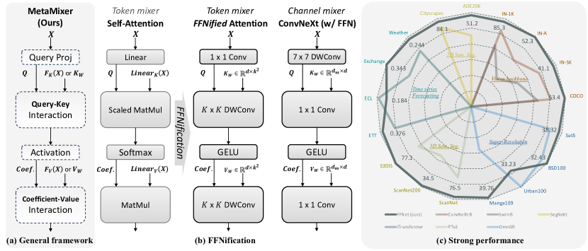
Figure 1: Overview of MetaMixer. (a) MetaMixer is derived by not specifying sub-operations within the query-key-value framework. We assert that the competence of Transformers primarily originates from MetaMixer, which we deem as the true backbone of Transformer. (b) To demonstrate this and propose a FFN-like efficient token mixer, we replace the inefficient sub-operations of self-attention with those from FFN while retaining MetaMixer structure. (c) Our MetaMixer-based pure ConvNets outperform domain-specialized competitors in various tasks, confirming the superiority of the MetaMixer framework.

1 Introduction

Transformer [94] models have emerged as the dominant backbone in Natural Language Processing (NLP) and have successfully extended their influence to the vision domains. The pioneering work of Vision Transformer (ViT) [27] and its follow-ups [7, 12, 59] have showcased promising performances in various vision tasks, posing a formidable challenge to the established Convolutional Neural Networks (CNNs) [34, 44]. Main component of the Transformer encoder, global self-attention, is specialized in modeling long-range dependencies but incurs a quadratic computational complexity with respect to the sequence length (resolutions). Therefore, deploying this module on resource-constrained mobile devices for real-time applications proves to be much more challenging than using lightweight CNNs. To address these issues, a lot of works have focused on modifying the self-attention module to be more vision-friendly [59, 65, 78, 32] or selectively applying it to low-resolution inputs [93, 111, 48, 107]. As such, effectively utilizing self-attention under strict latency constraints requires considerable efforts.

On the other hand, most models effortlessly leverage Feed-Forward Networks (FFNs, also known as channel MLP), which aggregate channel information with moderate computational overhead. Nevertheless, in vision domains, FFN is usually excluded from analysis, although there are several motivations to consider FFNs. For example, regardless of modality, whether generative or perception tasks, FFNs serve as a fundamental building block in transformer-based architectures, such as GPT series, ViT and its diffusion-based variants [2, 69]; this ubiquity suggests that FFNs play an indispensable role in achieving competitive performance. Furthermore, Geva et al. [30] suggest that FFNs can be viewed as emulated neural key-value memories [82, 83], where the rows in the first projection weights act as keys correlating with input textual patterns, and the rows in the second projection weights serve as values that induce a distribution shift over the residual path. Based on this intuition, if a depthwise convolution is used as query projection, ConvNeXt block [60] can also be interpreted as operating via a query-key-value mechanism, similar to the self-attention (see Fig. 1). We thus hypothesize that the query-key-value framework, fundamental to the most successful mixers like self-attention and ConvNeXt block, is essential as the starting point for mixer design.

We abstract the query-key-value mechanism into a generalized framework, MetaMixer, where sub-operations are not predefined, as illustrated in Fig. 1 (a). We further propose to replace the inefficient sub-operations of self-attention with those of FFN within the MetaMixer framework, aiming to bridge the efficiency gap between self-attention and FFN. We term it as FFNification. It consists of three aspects. (1) Key & Value Generation: Self-attention generates keys and values through linear projections (dynamic computation), whereas FFN employs static weights as keys and values. We thus adopt a static weight scheme for simple and efficient implementation. (2) Activation Function (Coefficient Generation): Attention softmax is costly because it involves calculating an exponent and summing across the token length, which poses challenges for parallelization [20]. Consequently, we replace the softmax with an element-wise activation function GELU [36]. (3) Query-Key-Value Interactions: The query-key and coefficient-value interactions in self-attention result in quadratic complexity $O(n^{2})$ with the token length $n$, as they compute relations between a single token and all other tokens. Instead, we explore whether these expensive calculations can be substituted by simple local aggregation like convolution. Inspired by large kernel CNNs [60, 26], we primarily use kernel sizes of 7 or even larger. The resulting FFNified attention and ConvNeXt block are symmetrical in terms of mixing dimension, and are thus adopted as the token mixer and channel mixer, respectively.

In this paper, we validate the MetaMixer framework by conducting extensive experiments across various tasks leveraging only convolutions. Astonishingly, as shown in Fig. 1 (c), our MetaMixer-based methods outperform domain-specialized competitors, requiring only minor task-specific modifications. Based on these results, we argue that MetaMixer stands as the pivotal mixer architecture that ensures competitive performance. We make the following contributions:

• We provide an in-depth analysis of the query-key-value mechanism of FFN in vision models (Sec. 2 and Appendix A) and further abstract this mechanism into a general mixer architecture MetaMixer that encompasses the main modules of both Transformer and ConvNeXt models (Sec. 3.1).

• Although self-attention and FFN-based convolutional mixers can both be integrated within the MetaMixer, a significant efficiency gap remains between them. To address this, we propose a mixer design that adapts self-attention by employing FFN’s sub-operations and mimicking its functionality through the use of large kernel convolutions (Sec. 3.2). The resulting token mixer, termed FFNified attention, not only surpasses the performance of attention-based mixers but also achieves remarkable inference speedups.

• Our methods achieve comprehensive state-of-the-art across a variety of modalities (image, point cloud, and time-series) and tasks (Sec. 4). We validate the efficacy of our approach on numerous tasks and comprehensively analyze the mixer design space through the MetaMixer framework (Appendix B, C).

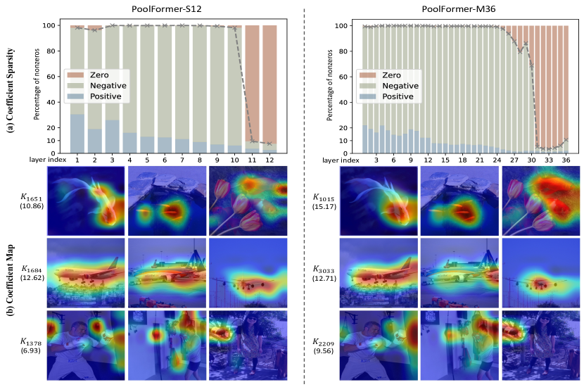
Figure 2: Key-Value Mechanism of FFNs in Visual Context. (a) Coefficient Sparsity: Astonishingly, the final stage shows significantly higher sparsity. To categorize numerous classes, a small subset (< 10%) of neurons are activated by the input. (b) Coefficient Map Corresponding to the Most Activated Key in the Last Layer: Keys specialized for each class selectively correlate at the target positions, suggesting their potential role in capturing distinctive visual features. The numbers in parentheses indicate the average values of the coefficients.

2 Feed-Forward Networks Are Key-Value Memories

Transformer block is primarily composed of self-attention module and Feed-Forward Network (FFN). Let $X\in\mathbb{R}^{n\times d}$ denote the input matrix, we can express self-attention and FFN as follows (bias terms, multi-head mechanism, and scaling factor in self-attention are omitted for simplicity):

$$Q=XW_{Q},K=XW_{K},V=XW_{V}$$ (2.1)

$$\mathrm{Attention}(X)=\mathrm{Softmax}(QK^{\top})V$$ (2.2)

$$\hskip 27.03003pt\mathrm{FFN}(X)=\mathrm{GELU}(XW_{1}^{\top})W_{2}$$ (2.3)

where $W_{1},W_{2}\in\mathbb{R}^{d_{m}\times d}$ and $W_{Q},W_{K},W_{V}\in\mathbb{R}^{d\times d_{h}}$. As shown in the above equations, the two projection weights of FFN operate similarly to the key-value in self-attention; the slight differences are that FFN is applied along the channel axis and uses GELU [36] instead of softmax. Specifically, the keys in $W_{1}$ detect patterns in the training samples, where $\textbf{c}=\mathrm{GELU}(XW_{1}^{\top})$ represents the unnormalized coefficients for each memory; then the values in $W_{2}$ are integrated by the corresponding memory coefficients. We refer to $\textbf{c}=\mathrm{GELU}(XW_{1}^{\top})$ as the coefficient.

Recent NLP literatures [30, 66, 18, 98] also delve into the knowledge (or skills) encoded within FFNs through viewing them as key-value memories [83]. For instance, Geva et al. [30] find that each key correlates with a range of human-interpretable patterns, from shallow to more semantic ones; Dai et al. [18] and Meng et al. [66] update specific factual associations by identifying and editing coefficients that express certain factual knowledge. Also, from a different perspective, recent studies find that coefficient sparsity in FFNs (with ReLU [29] inserted) is a prevalent phenomenon [49, 117], and utilizing sparsity after ReLU significantly reduces the computational requirements of LLMs [67].

While analyses of FFNs have reached maturity in NLP, the computer vision community lacks similar investigations. we thus analyze the FFNs within PoolFormer [110] from a key-value memory perspective. The simplicity of pooling as the token mixer makes FFN the dominant computational component in terms of parameter count and capacity, highlighting its crucial role in the model’s overall performance. As shown in Fig. 2 (a), similar to the observations in [67, 49], layers in the final stage have < 10% activated coefficients. Considering that each value can be interpreted as a distribution over the output prediction for classification [30], the result is intuitive. Also, the coefficient map examples in Fig. 2 (b) demonstrate that class-specific keys consistently correlate with target objects. Further examples and a more detailed discussion are provided in Appendix A. These results demonstrate that FFNs are indeed point-wise key-value memories, detecting and aggregating input patterns through interpretable inner workings. Therefore, it is noteworthy that the two main modules of Transformer operate within the query-key-value framework.

3 Method

3.1 MetaMixer

For the first time, we introduce the core concept “MetaMixer”. As shown in Fig. 1, MetaMixer is a flexible structure that does not specify sub-operations in the query-key-value framework [83, 94]. First, the query $q$ is generated by applying a projection layer to the input. Additionally, key-value pairs are either computed similarly to the query or randomly initialized as memory vectors, analogous to FFNs. We compute the match between $q$ and each key $k_{i}$ using a compatibility function (e.g., dot-product or convolution), followed by an activation function:

$$c_{i}=\mathrm{Activation}(f(q,k_{i}))$$ (3.1)

where $f(\cdot)$ is a compatibility function that computes the similarity between the query and the corresponding key (referred to as query-key interaction); $\mathrm{Activation}(\cdot)$ generates the coefficient $c$ on the values $v$. The output is then computed by an aggregation function $g(c,v)$ that sums the values, each weighted by the coefficient from Eq. 3.1. We refer to the process of aggregating values with their associated coefficients as coefficient-value interaction.

MetaMixer, as a general mixer architecture, can be instantiated as various well-established mixers by specifying sub-operations (query projection, key-value generation, query-key / coefficient-value interactions, and activation function). This nature demonstrates the capabilities of MetaMixer’s modular design. In Appendix B, we provide a detailed illustration of MetaMixer’s generality.

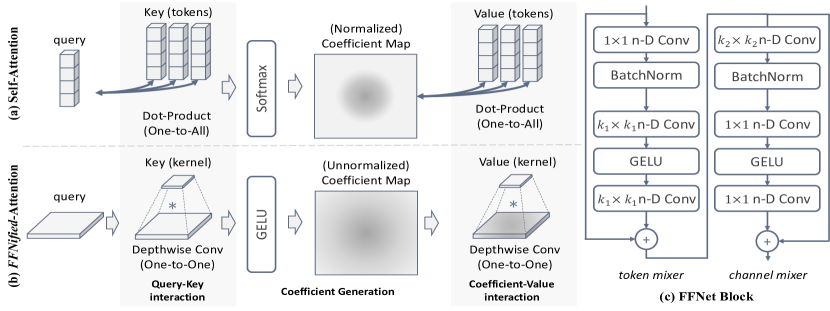
Figure 3: Overview of FFNification and Fast-Forward Network block. (a-b) Comparison between self-attention and FFNified attention; (c) Our mixer design easily adapts by selecting the convolution type based on the modality dimension.

3.2 FFNification

While in the Sec. 2, we have shown that both self-attention and FFN can be interpreted within the query-key-value mechanism, we note that self-attention (or local window-attention [59]) requires labor-intensive tuning and is less efficient in vision domains compared to FFN-based convolutional mixers [60, 85]. Hence, to incorporate the computational benefits of FFNs in diverse scenarios and further validate the significance of the MetaMixer beyond self-attention, we perform architectural surgeries that replace computationally intensive operations in self-attention with efficient alternatives. We refer to this process as FFNification. Specifically, we show that replacing the expensive pairwise dot-product in query-key/coefficient-value interactions with depthwise convolution is feasible, and that softmax is no longer an essential component.

The most critical aspect of the FFNification process is leveraging depthwise convolution for query-key and coefficient-value interactions. In self-attention, as inter-token module, each query (token) interacts with all instance-specific key-value pairs through dot-product operations. In contrast, with depthwise convolution, a query (channel) interacts with static key-value (kernel) in a sliding window manner. FFNified attention, therefore, utilizes key-value pairs to compute local similarities and aggregate information (see Fig. 3 (a-b)). Leveraging convolutional interaction is not only efficient but also benefits from inductive biases such as locality and weight sharing across positions, which reduces model complexity and aids in learning translationally equivalent representations. To enlarge the receptive field, we mainly utilize a 7$\times$7 kernel size for image recognition tasks, while for other tasks, the kernel size is adjusted based on the characteristics of the modality or task. Moreover, to enhance performance without increasing inference cost, we leverage a structural re-parameterization [25], training an additional small kernel branch (e.g., 3$\times$3) alongside a large kernel, which are subsequently merged into the large kernel during inference (see Appendix F for a detailed description).

While softmax self-attention has long been the de facto choice, its suitability in sparse computation scenarios like depthwise convolution warrants reconsideration. The exponential normalization in softmax tends to be highly centralized in a small number of values [61, 79, 5], which means convolution with a local receptive field may fail to achieve sufficient context aggregation. In contrast, GELU [36] do not suffer from this issue. Therefore, we adopt GELU in our settings.

The derived mixer, FFNified attention, along with the ConvNeXt block [60], consists solely of hardware-friendly operations such as convolution and GELU. Furthermore, within the MetaMixer framework, the FFNified attention and ConvNeXt block are symmetrically positioned to operate in opposite dimensions across each sub-operation (see Fig. 1 (b)). Consequently, we employ FFNified attention and the ConvNeXt block (7$\times$7 depthwise convolution + FFN) as token mixer and channel mixer, respectively. This arrangement facilitates efficient and compact feature extraction.

3.3 Fast-Forward Network as a General Backbone

Given our proposed FFNified attention and off-the-shelf ConvNeXt block as primary building mixers, we introduce Fast-Forward Network (FFNet), a new network family that demonstrates exceptional performance across a wide range of tasks with task-related modifications. The basic block of our FFNet is illustrated in Fig. 3 (c). Moreover, our model consists solely of hardware-friendly operations, ensuring high efficiency across various devices (GPU and Mobile device).

Our mixer design can be easily adapted to various modalities with minimal modifications. For image data, we utilize 2D depthwise convolution, while for time series analysis, 1D depthwise convolution is employed. For point clouds, we leverage 3D submanifold convolution [31], which introduces the hash table to retrieve input indices and processes only the non-empty elements, thus preserving the geometrical structure and maintaining low computation costs. Additionally, Batch Normalization (BN) [40] is primarily used as normalization layer, since BN can be merged into its adjacent convolution layer [25]. For more in-depth details regarding the specific adaptations for each task, please refer to the corresponding subsections.

4 Experimental Results

To demonstrate the versatility of our proposed method, we compare our Fast-Forward Network (FFNet) against the state-of-the-art baselines on diverse tasks such as image classification, object detection and instance segmentation, 2D semantic segmentation, super-resolution, 3D semantic segmentation, and long-term time series forecasting. Additional results can be found in the Appendix.

Speed Measurement. Following the same protocol as [93, 48], mobile latency is measured on iPhone 12 (iOS 16.5) using models exported by CoreML tools, while GPU throughput is measured with an NVIDIA RTX 4090 GPU. For throughput measurements on the GPU, we compile the traced model with TensorRT (v8.6.1.post1). Unless otherwise specified, all methods are evaluated using their respective input sizes and a batch size of 1, following the aforementioned procedure.

4.1 Image Classification

Table 1: ImageNet-1K classification results. We compare our models with state-of-the-art methods on ImageNet classification.“-” denotes that model could not be reliably exported by either TensorRT or Core ML Tools. The throughput/latency is measured with warmup and averaged over multiple runs.

Model Image Param FLOPs GPU Mobile Top-1 Size Throu. Latency Acc. (Px) (M) (G) (Img/Sec) (ms) (%) EfficientNet-B1 [85] $240^{2}$ 7.8 0.7 854 1.8 79.1 FastViT-SA12 [93] $256^{2}$ 10.9 1.9 731 2.0 80.6 Swin-T [59] $224^{2}$ 29.0 4.5 - 24.8 81.3 FFNet-1 $256^{2}$ 13.7 2.9 1113 1.8 81.3 DeiT3-S [90] $224^{2}$ 22.0 4.6 243 20.8 81.4 CoAtNet-0 [19] $224^{2}$ 25.0 4.2 - 8.2 81.6 CMT-XS [32] $192^{2}$ 15.2 1.5 424 3.9 81.8 ResNetV2-101 [100] $224^{2}$ 44.5 7.8 449 3.6 82.0 ConvNeXt-T [60] $224^{2}$ 29.0 4.5 789 3.7 82.1 PoolFormer-M48 [110] $224^{2}$ 73.5 11.6 - 7.7 82.5 FastViT-SA24 [93] $256^{2}$ 20.6 3.8 439 3.0 82.6 HorNet-T_7×7 [74] $224^{2}$ 22.0 4.0 428 3.4 82.8 EfficientNet-B4 [85] $380^{2}$ 19.3 4.2 572 5.2 82.9 Swin-S [59] $224^{2}$ 50.0 8.7 - 29.3 83.0 FFNet-2 $256^{2}$ 26.9 6.0 674 3.1 82.9 CoAtNet-1 [19] $224^{2}$ 42.2 8.4 - 17.0 83.3 MOAT-0 [107] $224^{2}$ 27.8 5.7 - 5.1 83.3 iFormer-S [81] $224^{2}$ 20.0 4.8 468 27.3 83.4 Swin-B [59] $224^{2}$ 87.8 15.4 - 33.5 83.5 CMT-S [32] $224^{2}$ 25.1 4.0 379 11.3 83.5 NFNet-F0 [4] $256^{2}$ 71.5 12.4 548 6.0 83.6 EfficientNet-B5 [85] $456^{2}$ 30.0 9.9 401 11.0 83.6 HorNet-S_7×7 [74] $224^{2}$ 49.5 8.8 331 5.4 83.8 ConvNeXt-B [60] $224^{2}$ 88.6 15.4 399 8.1 83.8 EfficientNetV2-S[86] $384^{2}$ 21.5 8.8 261 4.5 83.9 FastViT-MA36 [93] $256^{2}$ 42.7 7.9 314 4.7 83.9 FFNet-3 $256^{2}$ 48.3 10.1 490 4.5 83.9

Model Image Param FLOPs GPU Mobile Top-1 Size Throu. Latency Acc. (Px) (M) (G) (Img/Sec) (ms) (%) CoAtNet-2 [19] $224^{2}$ 75.0 15.7 - 24.4 84.1 HorNet-B_7×7 [74] $224^{2}$ 87.0 15.6 268 8.5 84.2 EfficientNet-B7 [85] $600^{2}$ 66.3 37.0 182 45.0 84.3 ConvNeXt-L [60] $224^{2}$ 198.0 34.4 206 16.5 84.3 CMT-B [32] $256^{2}$ 45.7 9.3 253 13.2 84.5 EfficientViT-L1 [5] $224^{2}$ 52.7 5.3 354 82.8 84.5 Swin-B [59] $384^{2}$ 88.0 47.1 - 181.6 84.5 FFNet-3 $\mathbf{384^{2}}$ 48.3 22.8 360 9.1 84.5 MOAT-0 [107] $384^{2}$ 27.8 18.2 - 25.2 84.6 iFormer-S [81] $384^{2}$ 20.0 16.1 328 80.3 84.6 NFNet-F1 [4] $320^{2}$ 132.6 35.5 278 15.8 84.7 NFNet-F2 [4] $352^{2}$ 193.8 62.6 186 27.0 85.1 EfficientNetV2-M[86] $480^{2}$ 54.0 24.0 199 11.0 85.1 CoAtNet-1 [19] $384^{2}$ 42.2 27.4 - 41.6 85.1 ConvNeXt-B [60] $384^{2}$ 88.6 45.0 220 21.3 85.1 HorNet-B_7×7 [74] $384^{2}$ 87.0 45.8 171 21.3 85.3 FFNet-4 $\mathbf{384^{2}}$ 79.2 43.1 264 15.2 85.3 ImageNet-1K distillation results SwiftFormer-L1 [78] $224^{2}$ 12.1 1.6 943 1.6 80.9 EfficientFormerV2-S2 [47] $224^{2}$ 12.6 1.3 671 2.0 81.6 FastViT-SA12 [93] $256^{2}$ 10.9 1.9 731 2.0 81.9 FFNet-1 $256^{2}$ 13.7 2.9 1113 1.8 82.1 SwiftFormer-L3 [78] $224^{2}$ 28.5 4.0 316 3.0 83.0 EfficientFormerV2-L [47] $224^{2}$ 26.1 2.6 542 2.8 83.3 FastViT-SA24 [93] $256^{2}$ 20.6 3.8 439 3.0 83.4 FFNet-2 $256^{2}$ 26.9 6.0 674 3.1 83.7 FFNet-3 $256^{2}$ 48.3 10.1 490 4.5 84.5

Architecture. Following convention, FFNet is structured into four stages, each consisting of multiple FFNet blocks for hierarchical feature extraction. In the token mixer, for efficiency, we adopt a kernel size of 3$\times$3 in the first two stages and switch to 7$\times$7 in later stages. In the channel mixer, we mainly use 7$\times$7 kernels, and the FFN’s expansion ratio is set to 3 by default ($d_{m}=3d$). The FFNet block is illustrated in Fig. 3 (c). For downsampling, we utilize a 7$\times$7 strided depthwise convolution followed by a 1$\times$1 convolution. We also use LayerScale [91] to make our deep models more stable during training. Model specifications are provided in Appendix G.1.

Setup. For image classification, we evaluate FFNet on the ImageNet-1K [23] dataset. We follow the same training recipe in  [89, 110] for a fair comparison. Specifically, we train our models for 300 epochs using AdamW optimizer with an initial learning rate of 1$\times 10^{-3}$ via cosine schedule and a weight decay of 0.05. We set the total batch size as 1024 and the input size as $256^{2}$. For $384^{2}$ resolution, we finetune the models for 30 epochs with weight decay 1$\times 10^{-8}$, learning rate of 5$\times 10^{-6}$, and batch size of 512. Following DeiT [89], we also report the results of hard distillation using RegNetY-16GF [73] (with top-1 accuracy of 82.9%) as the teacher model.

Table 2: COCO object detection and instance segmentation results using Cascade Mask R-CNN [6]. All backbone statistics are calculated with image size (1280, 800).

Backbone GPU Mobile $\text{AP}^{\text{box}}$ $\text{AP}^{\text{mask}}$ Throu. Latency Swin-T [59] 58 OOM 50.4 43.7 Swin-S [59] 34 OOM 51.9 45.0 ConvNeXt-T [60] 127 86.2 50.4 43.7 ConvNeXt-B [60] 54 173.1 52.7 45.6 HorNet-S_7×7 [74] 64 124.9 52.7 45.6 HorNet-B_7×7 [74] 44 182.2 53.3 46.1 FFNet-2 135 51.5 51.8 44.9 FFNet-3 90 80.5 52.8 45.6 FFNet-4 61 136.3 53.4 45.9

Results. In Tab. 1, we compare our models against recent state-of-the-art models. The comparison results clearly show that our FFNet obtains the best accuracy-speed trade-off on two different testbeds (GPU and mobile device). Notably, our model demonstrates a significant efficiency margin compared to attention-based models [32, 59, 81, 5], particularly on the mobile device. Furthermore, FFNet outperforms CNN-based models such as ConvNeXt and HorNet, which use kernels of the same size, thereby affirming the superiority of the proposed MetaMixer framework. Our model also generalizes well to a larger image resolution and distillation-based training [89].

4.2 Object Detection and Instance Segmentation

Setup. We evaluate the performance of FFNet as the backbone of Cascade Mask R-CNN [6] on the COCO object detection and instance segmentation tasks [52]. We adopt standard training recipe [59, 60] using 3$\times$ schedule with multi-scale training. All experiments are implemented on mmdetection [8] codebase.

Results. The results presented in Tab. 2 indicate that FFNet models outperform baselines across all scales. Remarkably, our models demonstrate impressive efficiency improvements compared to the baselines with similar performance.

4.3 2D Semantic Segmentation

Table 3: 2D semantic segmentation results. To facilitate a comprehensive evaluation of efficiency, we report backbone speed at the backbone-level and overall model speed at the system-level comparison. Backbone statistics are calculated with image size (2048, 512). The input size is (2048,1024) for Cityscapes. “SS”/“MS” denote single-scale and multi-scale testing, respectively. “$*$” indicates use of an RTX A6000 GPU.

Backbone Param FLOPs GPU Mobile mIoU Throu. Latency (M) (G) (Img/Sec) (ms) (SS/MS) Backbone-Level Comparison on ADE20K with UperNet 160K Swin-T [59] 60 945 60 OOM 44.5 / 45.8 Swin-B [59] 121 1188 28 OOM 48.1 / 49.7 ConvNeXt-T [60] 60 939 119 70 46.0 / 46.7 ConvNeXt-B [60] 122 1170 40 170 49.1 / 49.9 HorNet-S_7×7 [74] 81 1030 57 112 49.2 / 49.8 HorNet-B_7×7 [74] 121 1174 37 169 50.0 / 50.5 HorNet-B_GF [74] 126 1171 - - 50.5 / 50.9 FFNet-2 58 942 135 45 47.1 / 47.8 FFNet-3 80 1010 90 69 49.6 / 50.2 FFNet-4 113 1158 60 124 50.7 / 51.7

Model Param FLOPs GPU* mIoU Latency (M) (G) (ms) (SS/MS) System-Level Comparison on ADE20K SETR-MLA [120] 310 368 82 47.5 / 49.4 Segformer-B3 [106] 47 79 256 49.4 / 50.0 MaskFormer [12] 63 79 - 49.8 / 51.0 SegNeXt-B [33] 28 35 127 48.5 / 49.9 EfficientViT-L1 [5] 40 36 80 49.2 / - $\text{FFNet}_{\textit{seg}}$ 68 74 65 50.1 / 51.2 System-Level Comparison on Cityscapes Segformer-B3 [106] 47 963 252 81.7 / 83.3 SegNeXt-L [33] 49 578 307 83.2 / 83.9 $\text{FFNet}_{\textit{seg}}$ 68 577 224 83.2 / 84.1

Architecture. For comparison at the backbone level, we utilize ImageNet-pretrained models as the backbone of UperNet [105]. Furthermore, to enable a system-level comparison, we propose $\text{FFNet}_{\textit{seg}}$, a model similar to the original FFNet but incorporating task-specific modifications. $\text{FFNet}_{\textit{seg}}$ adopts the standard backbone-head (encoder-decoder) architecture. Similar to the backbone, the head also employs FFNet blocks, thereby avoiding complex operations such as global self-attention [12] and matrix decomposition [33]. Following  [33], we input the features from the last three stages into the head, where they are concatenated and processed through an FFN. Detailed configurations of the head for each datset will be provided in our official GitHub repository.

Recent works [5, 33, 118] demonstrate that long-range interactions and multi-scale features are crucial for competitive performance in segmentation models. Accordingly, to enlarge the receptive field, we employ 9$\times$9 kernels in the final two stages of the backbone and the head. Additionally, to effectively process features of objects with varying sizes, we combine small-kernel and strip convolutions [38, 71] (9$\times$1, 1$\times$9) with large-kernel convolution, enhancing flexible feature extraction. Further details and a visual schematic can be found in Appendix F and Tab. 10.

Setup. We evaluate the effectiveness of our FFNet on two representative benchmark datasets: ADE20K [121] and Cityscapes [16]. For backbone-level comparison, our models are trained for 160K-iterations with a batch size of 16, following standard recipe [59, 60]. For system-level comparisons, we adopt the same training settings in SegNeXt [33] and use ImageNet-1K pretrained models for initialization. We also use MMSegmentation toolbox [14] for all semantic segmentation experiments.

Results. Tab. 3 shows that our methods excel not only as backbones but also as standalone segmentors, highlighting our model’s superior performance-speed trade-off. For example, FFNet-4 achieves a $+1.8$ mIoU gain over ConvNeXt-B, while providing 50% improvement in GPU speed and 37% increase in mobile speed. Also, $\text{FFNet}_{\textit{seg}}$ consistently outperforms task-specific prior arts.

4.4 Super-Resolution

Architecture. $\text{FFNet}_{\textit{sr}}$ consists of three parts: shallow feature extractor (H_SF), deep feature extractor (H_DF), and upscale module (H_Rec) following residual-in-residual architecture [115]. H_SF extracts shallow features from a Low-Resolution (LR) image using a 3$\times$3 convolution. The deep feature extractor H_DF, comprising a stack of FFNet blocks, refines shallow features iteratively. Specifically, $\text{FFNet}_{\textit{sr}}$-light and $\text{FFNet}_{\textit{sr}}$ employ 36 and 48 blocks, respectively. We use 3$\times$3 depthwise convolutions across all variants, with 96 base channels and an FFN expansion ratio of 2. In line with findings from EDSR [51], we also observe similar performance degradation when using Batch Normalization (BN) and consequently exclude BN from the FFNet Block. We use anchor-based long residual connection [28, 125] where the LR image is repeated RGB-wise and added at the end of the H_DF. Finally, H_Rec reconstructs the High-Resolution image by up-sampling refined features (see Appendix G.2 for more details).

Setup. $\text{FFNet}_{\textit{sr}}$-light and $\text{FFNet}_{\textit{sr}}$ is evaluated on the DIV2K [51] and DF2K (DIV2K + Flicker2K [87]) dataset, respectively. Five standard datasets are adopted for testing: Set5 [3], Set14 [113], BSD100 [63], Urban100 [39], and Manga109 [64]. We use PSNR and SSIM to evaluate the SR performance on the Y channel from the YCbCr color space after cropping 2 pixels at boundary [41]. In each training batch, we randomly crop LR patches of size 96$\times$96 as input and augment the patches with random horizontal flip and rotations. Our models are trained by minimizing L1 loss and frequency reconstruction loss [92, 84] with a weight factor 0.02. We use Adam optimizer for training with a batch size 64 for 500K iterations. The initial learning rate is set to 0.001 and updated by the cosine annealing scheme. All latency and memory usage are measured corresponding to an HR image of size 1280$\times$720.

Results. In Tab. 4, we compare our models against recent state-of-the-art SR models. Notably, $\text{FFNet}_{\textit{sr}}$ significantly outperforms SR specialists in efficiency, operating seamlessly even on resource-constrained devices, demonstrating their feasibility for real-world applications. $\text{FFNet}_{\textit{sr}}$, employing 3$\times$3 convolutions within the MetaMixer framework, not only captures high-frequency details effectively but also allows for the stacking of more blocks within the same computational budget compared to the baselines [84, 11, 95] that use complex mixers, thereby enhancing its ability to capture long-range contexts. The impressive results suggest that our mixer design is not only effective for high-level tasks such as recognition but also well-suited for solving low-level problems. Visual results of the $\text{FFNet}_{\textit{sr}}$ are provided in Appendix I.

Table 4: Comparisons on representative benchmark datasets for Super-Resolution networks at $\times$2 scale. All results are calculated on the Y-channel. All statistics are calculated corresponding to an HR image of size 1280$\times$720. Memory denotes maximum GPU memory consumption during the inference phase. Best and second-best results are bolded and underlined, respectively. $\dagger$ denotes we re-implement model since their codes are unavailable.

Methods	Published	Memory (mb)	Latency			Dataset	Performance (PSNR/SSIM) $\uparrow$
			RTX4090 (ms)	iPhone12 (sec.)	M2Air (sec.)		Set5	Set14	B100	Urban100	Manga109
EDSR [51]	CVPRW17	1488.4	196.6	3.6	1.4	DIV2K	38.11/0.9602	33.92/0.9195	32.32/0.9013	32.93/0.9351	39.10/0.9773
SwinIR-light [50]	ICCVW21	1764.3	124.9	OOM	OOM		38.14/0.9611	33.86/0.9206	32.31/0.9012	32.76/0.9340	39.12/0.9783
ELAN-light [114]	ECCV22	687.0	50.2	OOM	OOM		38.17/0.9611	33.94/0.9207	32.30/0.9012	32.76/0.9340	39.11/0.9782
DITN† [56]	MM23	679.1	62.8	OOM	OOM		38.17/0.9611	33.79/0.9199	32.32/0.9014	32.78/0.9343	39.21/0.9781
SwinIR-NG [13]	CVPR23	1712.4	143.9	-	-		38.17/0.9612	33.94/0.9205	32.31/0.9013	32.78/0.9340	39.20/0.9781
$\text{FFNet}_{\textit{sr}}$-light	-	394.1	55.3	1.0	0.4		38.23/0.9613	33.75/0.9204	32.34/0.9018	32.81/0.9344	39.23/0.9781
OmniSR [95]	CVPR23	892.2	76.6	-	-	DF2K	38.29/0.9617	34.27/0.9238	32.41/0.9026	33.30/0.9386	39.53/0.9792
EDT-T [46]	IJCAI23	5364.7	334.1	-	-		38.23/0.9615	33.99/0.9209	32.37/0.9021	32.98/0.9362	39.45/0.9789
DAT-light [11]	ICCV23	2295.2	1936.3	OOM	OOM		38.24/0.9614	34.01/0.9214	32.34/0.9019	32.89/0.9346	39.49/0.9788
SAFMN-large [84]	ICCV23	767.5	124.9	OOM	0.8		38.28/0.9616	34.14/0.9220	32.39/0.9024	33.06/0.9366	39.56/0.9790
$\text{FFNet}_{\textit{sr}}$	-	397.6	72.3	1.4	0.6		38.32/0.9618	34.28/0.9235	32.43/0.9029	33.23/0.9382	39.76/0.9793

4.5 3D Semantic Segmentation

Architecture. Following [104], we adopt the U-Net [76] structure, comprising four stages of encoders and decoders with block depths of [2, 2, 6, 2] and [1, 1, 1, 1], respectively. We also utilize the Grid Pooling introduced in [104], setting all grid size multipliers to $\times$2, which represents the expansion ratio over the preceding pooling stage. For token mixing, we employ submanifold convolution [31]. Additionally, to manage memory-constrained scenarios requiring small batch sizes, we use both batch normalization and pre-norm (layer normalization) scheme. Due to the implementation limitations of submanifold convolution, which does not support depthwise operation, we restrict our kernel size to 3$\times$3 to handle overfitting issues. Despite these constraints, the obtained results are promising, demonstrating that even small kernels are highly effective within the U-Net structure. Detailed descriptions of architecture can be found in Appendix G.3.

Table 5: Multivariate time series long-term forecasting results with prediction lengths $S\in\{96,192,336,720\}$ and fixed lookback length $T=96$. Results are averaged from all prediction lengths. ETT results further averaged by subsets. The baseline numbers are from [57]. The best results are in bold and the second best are underlined.

Models	FFNet		iTransformer		PatchTST		Crossformer		TiDE		TimesNet		DLinear		SCINet		FEDformer		Stationary		Autoformer
	(Ours)		[57]		[68]		[116]		[22]		[101]		[112]		[53]		[124]		[58]		[102]
Metric	MSE	MAE	MSE	MAE	MSE	MAE	MSE	MAE	MSE	MAE	MSE	MAE	MSE	MAE	MSE	MAE	MSE	MAE	MSE	MAE	MSE	MAE
ETT	0.376	0.390	0.383	0.399	0.381	0.397	0.685	0.578	0.482	0.470	0.391	0.404	0.442	0.444	0.689	0.597	0.408	0.428	0.471	0.464	0.465	0.459
ECL	0.184	0.278	0.178	0.270	0.205	0.290	0.244	0.334	0.251	0.344	0.192	0.295	0.212	0.300	0.268	0.365	0.214	0.327	0.193	0.296	0.227	0.338
Exchange	0.343	0.392	0.360	0.403	0.367	0.404	0.940	0.707	0.370	0.413	0.416	0.443	0.354	0.414	0.750	0.626	0.519	0.429	0.461	0.454	0.613	0.539
Traffic	0.517	0.338	0.428	0.282	0.481	0.304	0.550	0.304	0.760	0.473	0.620	0.336	0.625	0.383	0.804	0.509	0.610	0.376	0.624	0.340	0.628	0.379
Weather	0.244	0.274	0.258	0.278	0.259	0.281	0.259	0.315	0.271	0.320	0.259	0.287	0.265	0.317	0.292	0.363	0.309	0.360	0.288	0.314	0.338	0.382

Table 6: 3D semantic segmentation results.

3D Sem. Seg. ScanNet [17] ScanNet200 [77] S3DIS [1] Model Val Test Val Test Area5 6-fold PointNeXt [72] 71.5 71.2 - - 70.5 74.9 ST [45] 74.3 73.7 - - 72.0 - OctFormer [97] 75.7 76.6 32.6 32.6 - - Swin3D [109] 76.4 - - - 72.5 76.9 OA-CNNs [70] 76.1 75.6 32.3 33.3 71.1 - PTv2 [104] 75.4 74.2 30.2 - 71.6 73.5 FFNet 76.1 76.5 33.8 34.5 72.6 77.1

Setup. We conduct experiments using our models on the representative datasets: ScanNetv2 [17], ScanNet200 [77], and the S3DIS [1] for indoor scenes. We use Pointcep [15] codebase specialized for point cloud perception tasks. Details on the training settings are provided in Appendix H.1.

Results. Remarkably, simply adapting our methods to point clouds demonstrates superior performance compared to task-specific competitors, as shown in Tab. 6. We anticipate that incorporating adaptive convolution [70] or large kernel convolution [10] to our mixer design could further enhance performance.

4.6 Time-Series Forecasting

Architecture. For time-series forecasting, we employ a backbone-head structure with RevIN [42], where the backbone consists of stacked FFNet blocks. In our mixer design, we utilize a 51-sized kernel for depthwise convolution to effectively catch up the global receptive fields of transformer-based and MLP-based models. In fact, directly applying the FFNet block (Fig. 3 (c)) to time series data is challenging due to the presence of variable dimension in addition to channel and temporal dimensions in multivariate setting. To effectively capture both temporal and cross-variable dependencies, we modify FFN part using appropriate grouping and feature reshaping. Detailed descriptions of these time series-specific modifications and architecture details are available in Appendix G.4.

Setup. We conduct long-term forecasting experiments on popular 8 real-world datasets, including ETT (4 subsets), ECL, Exchange, Traffic, Weather. Following [57], we set the input length as 96 for all the results. We compute the Mean Squared Error (MSE) and Mean Absolute Error (MAE) as metrics for multivariate time series forecasting. Detailed settings are provided in Appendix H.2.

Results. Tab. 5 shows the comparable performance of FFNet in multivariate time-series forecasting. Specifically, FFNet consistently outperforms recent state-of-the-art transformer-based and MLP-based models in most cases, demonstrating the excellent task-generality of our approach.

5 Conclusion

In this work, we analyzed the FFN from a seldom-explored perspective and integrated self-attention and FFN-based mixers within a query-key-value framework. We further abstracted this framework into a general mixer architecture, termed MetaMixer, where sub-operations are unspecified. Based on the MetaMixer, we presented a convolutional mixer design with FFNified attention. In numerous tasks where transformer-based and convolution-based models are in fierce competition, we merge both approaches in a completely new direction, and achieve a new state of the art. This achievement underscores that the significance lies not in self-attention per se, but in satisfying task-specific functionalities, starting with MetaMixer as the foundation.

Appendix A FFNs Are Key-Value Memories

In this section, we conduct an in-depth analysis of the Feed-Forward Network (FFN) within the trained vision model PoolFormer-M36 [110]. We identify the most activated keys on average for each class using the ImageNet-1K validation set. Surprisingly, keys specialized for each class demonstrate a human-interpretable correlation in semantically consistent regions, following the point-wise mechanism of the FFN (see Fig. 5 (a)). Moreover, these keys operate not in isolation but in a hierarchical and composite manner. For instance, certain keys are associated with higher-level concepts shared across classes, such as animal species and machine parts (see Fig. 5 (b)). Furthermore, we discover keys that strongly correlate with approximately 70% to 85% of the classes. For example, $K_{10}$ correlates with the surroundings of the target object, aiding in shape recognition (see Fig. 7 (a)), while $K_{1395}$ correlates with a wide range of objects, serving as a detector of objectness (see Fig. 7 (b)).

We also find that $K_{548}$ and $K_{1461}$ from the smaller variant PoolFormer-S12, as well as $K_{382}$ and $K_{2869}$ from the ViT-B trained on ImageNet-21K, operate similarly to the special keys discussed above. Additionally, Li et al. [49] observed that the FFN’s activations in ViT models are sparse, mirroring observations in Fig. 2 (a). The above results suggest that FFNs generally operate as key-value memories across various models.

Interestingly, as shown in Fig. 6, class-specific keys in ViT-B not only correlate locally with the target object but also with its immediate surroundings and low-informative background areas. This could be related to unexpected behaviors observed in attention layers, such as artifacts in attention maps [21] and query-irrelevant attentions [62]. Consequently, similar to previous work [43] that analyzed internal processing of FFNs in BERT and GPT-2 through attention maps, investigating FFN’s key-value mechanism in relation to attention layers in vision models is also a promising future research direction.

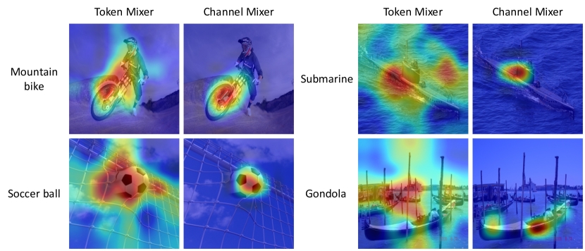
Figure 4: Examples of coefficient maps corresponding to the most activated key from the mixers in the final block of FFNet-3.

In Fig. 4, we also present the coefficient maps of FFNet-3. Within the token mixer, the keys correlate with both the target object and its surrounding context, whereas in the channel mixer, the focus is centralized on the target object. This demonstrates a complementary mechanism where the token mixer uses a large kernel to aggregate surrounding context, followed by the channel mixer concentrating on critical regions.

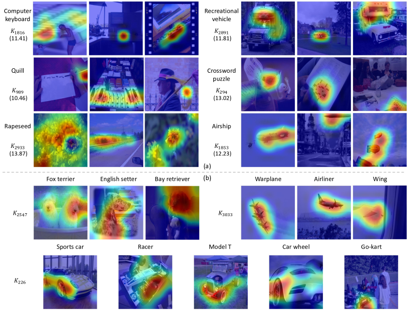
Figure 5: Visualization of the FFN’s coefficient map in the last layer of PoolFormer-M36 [110]. (a) We visualize coefficient maps corresponding to the most activated keys for each class, where class-specific keys consistently correlate with decisive locations. The numbers in parentheses indicate the average values of the coefficients. (b) We identify keys that detect concepts shared across classes, such as animal species and machine parts, revealing that the keys capture patterns in the input through a hierarchical manner. Specifically, $K_{226}$ is mostly inactive except in classes that include wheels.

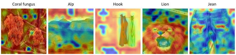
Figure 6: Coefficient maps from ViT-B [27] trained on ImageNet-21K. These examples exhibit behavioral patterns distinctly different from those observed in PoolFormer models, indicating a need for analysis alongside preceding attention layers. Detailed discussion is beyond the scope of this paper and is therefore omitted.

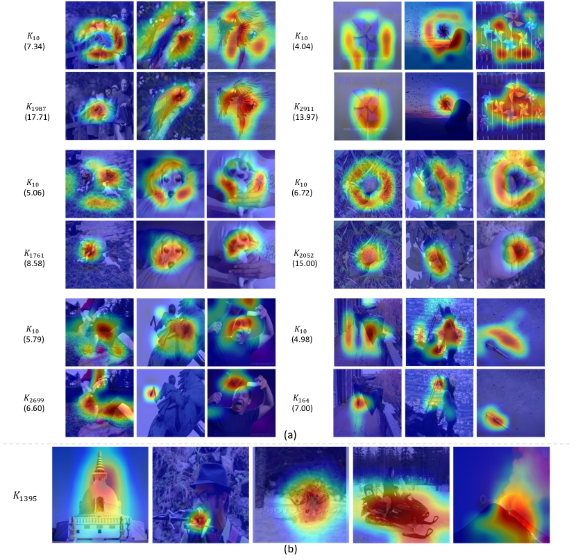
Figure 7: We analyze two representative class-agnostic keys in the last layer of PoolFormer-M36. $K_{10}$ and $K_{1395}$ are included in the most activated top-5 keys at rates of 71.7% and 84.6%, respectively. (a) $K_{10}$ correlates with the surrounding context of the target object, capturing its shape and aiding in context comprehension. The numbers in parentheses indicate the average values of the coefficients. (b) $K_{1395}$ consistently correlates across various types of objects.

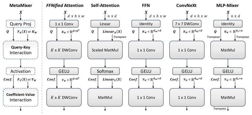
Figure 8: Generality of the MetaMixer. The notation for each mixer follows that introduced in its respective seminal paper. The variables $d$, $d_{m}$, $d_{s}$, and $n$ represent the base channel dimension, hidden dimension, hidden dimension of the spatial MLP, and token length (resolution), respectively. For ease of comparison, normalization layers are omitted. The MetaMixer framework encompasses the most successful mixers, demonstrating its modular nature.

Appendix B MetaMixer Generality

As shown in Fig. 8, the most commonly used mixers are instantiated by specifying sub-operations of the MetaMixer, underscoring that the query-key-value mechanism is a essential requirement for competitive performance. Specifically, The spatial MLP in MLP-Mixer [88] operates via the same query-key-value mechanism as an FFN, but applies it along different axes—token and channel, respectively. The ConvNeXt [60] block can be interpreted as employing a 7$\times$7 depthwise convolution as the query projection layer within an FFN. Additionally, self-attention and FFNified attention utilize inter-token matrix multiplication and depthwise convolution, respectively, to compute query-key-value interactions.

Appendix C Detailed Comparisons with Related Work

MLP-Mixer. The term “FFNification” might initially evoke thoughts of spatial MLPs [88] rather than our proposed FFNified attention due to its direct implications. However, our use of the term encompasses not only the adaptation of mechanisms but also aims to achieve the generality and efficiency characteristic of FFNs. Spatial MLPs, on the other hand, suffer from parameter inefficiency [88, 119] and are impractical for high-resolution inputs, similar to the global self-attention. They also unable to handle multiple resolutions, limiting their applicability across various tasks. Consequently, depthwise convolution emerges as an efficient and effective alternative, addressing these issues. Unlike spatial MLPs, which share the same kernel across all channels, depthwise convolution applies different kernels to each channel. To bridge the receptive field gap between convolution and spatial MLP, we employ large kernels (e.g., 7$\times$7 or 9$\times$9 for image recognition and 51 for time series).

ConvNeXt. Both the ConvNeXt [60] block and FFNified attention mixer share basic elements such as convolution and GELU activation, yet they differ in the operating axes of the query-key-value mechanism. FFNified attention actively extracts spatial features through two consecutive large-kernel convolutions, calculating query-key and coefficient-value interactions. In contrast, the ConvNeXt block uses depthwise convolution as a means of query projection, indirectly utilizing the surrounding context during channel interaction. Hence, employing our proposed FFNified attention and ConvNeXt block as token mixer and channel mixer, respectively, provides a compact mixer design space. In FFNified attention, it is natural to not expand channels, leading our FFNet to maintain a larger base channel size compared to similar-sized baseline models and thus reduce the expansion ratio in the channel mixer to 3. This decision aligns with prior research findings [55] that the expanded features of channel mixer contain substantial redundancy. Thanks to our comprehensive design strategy and compact mixer space, our models demonstrate a better performance-speed trade-off than the ConvNeXt models especially on resource-constrained devices. (see Tab. 7).

ViT and Swin Transformer. Self-attention operates at the token level, employing matrix multiplication to calculate inter-token similarity and aggregate values using the resulting coefficients. In contrast, FFNified attention operates at the channel level, detecting local patterns through depthwise convolution and applying a subsequent convolution to the resulting coefficients to aggregate values. To reduce parameter complexity, self-attention shares attention weights across channels, while FFNified attention shares them across positions. Another key difference lies in the key-value generation process: self-attention utilizes instance-specific key-value pairs through linear projections, while FFNified attention initializes key-values as static weights and updates them on the training set.

Vanilla self-attention, being a token-based module, faces limitations in vision tasks with long token lengths. Swin transformer [59] addresses this by performing self-attention within local windows. However, window attention necessitates complex reshape operations, hindering efficient deployment across various inference platforms [55, 111]. Conversely, FFNified attention, composed solely of hardware-friendly operations like convolution and GELU, exhibits high speed across diverse devices (see Tab. 7).

Table 7: Comparison of inference speeds across various hardware platforms for FFNet, Swin Transformer, and ConvNeXt. “bs” denotes batch size. For CPU benchmarks, models are converted to ONNX runtime format and evaluated on an Intel(R) Xeon(R) Gold 5218R CPU @ 2.10GHz processor using a single thread. For Mobile and M2Air, we export the models using CoreML tools and report the median latency over 1,000 runs.

Model Top-1 GPU Throughput (img/sec) CPU Throughput (img/sec) Mobile Macbook Air (%) bs 1 bs 64 bs 1 bs 16 Latency (ms) Latency (ms) Swin-T 81.3 - 1934 30 35 24.8 6.9 ConvNeXt-T 82.1 789 2397 40 48 3.7 2.4 FFNet-2 82.9 674 2142 28 52 3.1 2.1 Swin-B 83.5 - 841 13 14 33.5 12.1 ConvNeXt-B 83.8 399 1246 16 17 8.1 5.6 FFNet-3 83.9 490 1420 20 40 4.5 2.9

Appendix D Effective Receptive Field (ERF)

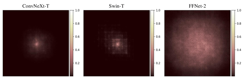
Model	t=20%	t=30%	t=50%	t=99%
ConvNeXt-T	1%	1.6%	4.4%	53.2%
Swin-T	1.6%	2.9%	6.5%	60.3%
FFNet-2	10.4%	16.4%	30.2%	97.9%

Figure 9: Left. Effective receptive field (ERF) comparison. FFNet has broader ERFs compared to Swin Transformer and ConvNeXt, despite using the same kernel (window) size. Right. Quantitative analysis on the ERF with the high-contribution area ratio $r$. A higher value of $r$ indicates a smoother distribution of high-contribution pixels, which implies a larger ERF.

Previous works [24, 54] have identified the Effective Receptive Field (ERF) as a key factor in enhancing CNN performance, scaling kernels up to 31$\times$31 or even 51$\times$51. In this section, we compare the ERFs of ConvNeXt and Swin Transformer, which use the same kernel (window) size, with our FFNet. Following RepLKNet [24], we sample and resize 50 images from the ImageNet validation set to 1024 $\times$ 1024, and measure the contribution of pixels on the input images to the central point of the feature map produced by the last layer. Contributions are aggregated and mapped onto a 1024 $\times$ 1024 matrix. We further quantify the ERF of each model by calculating the high-contribution area ratio $r$ of a minimum rectangle that encompasses the contribution scores over a certain threshold $t$. As depicted in Fig. 9, while high-contribution pixels in ConvNeXt and Swin are concentrated around the center of the input, FFNet’s high-contribution pixels are dispersed across a wider ERF. These results demonstrate that our model more effectively utilizes convolutions with the same kernel size to consider a larger range of pixels for final predictions. These results are consistent with the examples in Fig. 4.

Table 8: Robustness evaluation of FFNet. “$*$” indicates that model is trained using DeiT [89] distillation.

Model #Params. GPU Throughput Mobile Latency IN-Clean IN-A [37] IN-R [35] IN-SK [96] IN-V2 [75] (M) (img/sec) (ms) Top-1 (%) Top-1 (%) Top-1 (%) Top-1 (%) Top-1 (%) FastViT-SA12 [93] 10.9 731 2.0 80.6 17.2 42.6 29.7 - FFNet-1 13.7 1113 1.8 81.3 18.8 44.1 31.6 70.1 FFNet-1^∗ 13.7 1113 1.8 82.1 24.2 47.0 33.5 71.5 Swin-T [59] 29.0 - 24.8 81.3 21.6 41.3 29.1 69.7 ConvNeXt-T [60] 28.6 789 3.7 82.1 24.2 47.2 33.8 71.0 FocalNet-T (LRF) [108] 28.6 599 4.3 82.3 23.5 45.1 31.8 71.2 EfficientNet-B4 [85] 19.3 572 5.2 82.9 26.3 47.1 34.1 72.3 FFNet-2 26.9 674 3.1 82.9 27.3 48.0 34.6 71.8 FFNet-2^∗ 26.9 674 3.1 83.7 33.4 51.3 37.8 73.3 Swin-B [59] 87.8 - 33.5 83.5 35.8 46.6 32.4 72.3 ConvNeXt-S [60] 50.2 459 5.0 83.1 31.3 49.6 37.1 72.5 ConvNeXt-B [60] 88.6 399 8.1 83.8 36.7 51.3 38.2 73.7 FastViT-MA36 [93] 42.7 314 4.7 83.9 34.6 49.5 36.6 - FocalNet-B (LRF) [108] 88.7 278 10.0 83.9 38.3 48.1 35.7 73.5 FFNet-3 48.3 490 4.5 83.9 36.2 50.8 37.6 73.4 FFNet-3^∗ 48.3 490 4.5 84.5 39.5 54.1 40.2 74.5 ImageNet-1K 384 $\times$ 384 fine-tuned models Swin-B [59] 87.8 - 181.6 84.5 42.0 47.2 33.4 73.2 ConvNeXt-B [60] 88.6 220 21.3 85.1 45.6 52.9 39.5 75.2 FFNet-4 79.2 264 15.2 85.3 52.3 54.8 41.1 76.0

Appendix E Robustness Evaluation

In this section, we test our models on several robustness benchmark datasets: ImageNet-A [37], a test set comprising natural adversarial examples; ImageNet-R [35], an extended test set containing samples that are misclassified by ResNet-50 [34]; ImageNet-Sketch [96], comprised solely of hand-drawn images, serves as an effective test set for classification capabilities in the absence of texture or color information; and ImageNet-V2 [96], an extended test set that employs the same sampling strategy as ImageNet-1K.

Robustness evaluation results are presented in Tab. 8. Our models exhibit promising robust performance, outperforming well-tuned models on four additional test sets. With distillation, FFNets show strong generalization capabilities across all scales. Notably, on the most challenging test set, ImageNet-A, FFNet-4 achieves a 52.3% accuracy, surpassing Swin-B and ConvNeXt-B by 10.3% and 6.7%, respectively.

Appendix F Structural Re-parameterization

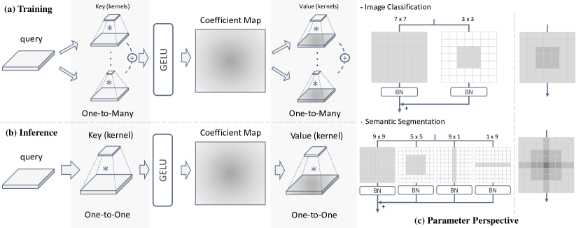
Figure 10: Visual explanation of re-parameterizing multi-branches for extracting multi-scale features. For a detailed discussion, refer to Appendix F.

Structural re-parameterization [25] is a methodology that transforms train-time multi-branch architectures into plain architectures through parameter transformation. We utilize this methodology to incorporate small kernels (e.g., 3$\times$3 or 5$\times$5) into larger ones (e.g., 7$\times$7 or 9$\times$9), as shown in Fig. 10. Additionally, for semantic segmentation model FFNet_seg, we add 9$\times$1 and 1$\times$9 convolution branches to effectively extract features of strip-like objects, such as human and tree. This approach enables our mixer to capture patterns of various scales and aspect ratios.

Using multi-branches can be interpreted as one-to-many interactions, similar to the self-attention, leveraging multiple key-value pairs for a single query. However, unlike self-attention, which typically considers a large number of key-values (e.g., 196 or 49 tokens) per query, our method uses only 2 or 4 key-values, making element-wise addition followed by GELU (“collaborative weighting”) more natural than softmax (“competitive weighting”). Meanwhile, based on FFNified attention, leveraging softmax gating with multi-branches for context-dependent key-values [9] or handling multiple tasks [122] presents an intriguing direction for future research. As demonstrated in Tab. 9, employing the re-parameterization technique within our mixer design effectively boosts performance without additional inference costs. However, this technique results in increased training time due to the added branches.

Table 9: Comparison of FFNet models with and without multi-branches using re-parameterization technique when trained on ImageNet-1K. Train time refers to the wall clock time elapsed at the end of a training run, as measured using 8 RTX A6000 GPUs.

Variant Ablation Train Time (hrs) Top-1 Acc. (%) FFNet-1 plain architecture 34.5 81.0 multi-branches w/ re-param. 36.6 81.3 FFNet-2 plain architecture 73.2 82.5 multi-branches w/ re-param. 77.5 82.9

Appendix G Architecture Details

G.1 ImageNet Classification Model Architecture Details

Table 10: Details about FFNet’s architecture for ImageNet classification. The expansion ratio in the channel mixer of $\text{FFNet}_{\textit{seg}}$ is set to 4, while for all other variants (FFNet-1 $\sim$ 4), it is set to 3.

Output size	Layer	FFNet-1	FFNet-2	FFNet-3	FFNet-4	$\text{FFNet}_{\textit{seg}}$
$\frac{H}{4}\times\frac{W}{4}$	stem	$3\times 3$, $64$, s = 2 $3\times 3$, $80$, s = 2	$3\times 3$, $64$, s = 2 $3\times 3$, $88$, s = 2	$3\times 3$, $64$, s = 2 $3\times 3$, $96$, s = 2	$3\times 3$, $64$, s = 2 $3\times 3$, $128$, s = 2	$3\times 3$, $64$, s = 2 $3\times 3$, $64$, s = 1 $3\times 3$, $96$, s = 1 $3\times 3$, $96$, s = 2
$\frac{H}{4}\times\frac{W}{4}$	token mixer channel mixer	$\begin{bmatrix}\begin{array}[]{c}3\times 3,80\\ 3\times 3,80\end{array}\end{bmatrix}\times 2$	$\begin{bmatrix}\begin{array}[]{c}3\times 3,88\\ 7\times 7,88\end{array}\end{bmatrix}\times 3$	$\begin{bmatrix}\begin{array}[]{c}3\times 3,96\\ 7\times 7,96\end{array}\end{bmatrix}\times 4$	$\begin{bmatrix}\begin{array}[]{c}3\times 3,128\\ 7\times 7,128\end{array}\end{bmatrix}\times 4$	$\begin{bmatrix}\begin{array}[]{c}3\times 3,96\\ 3\times 3,96\end{array}\end{bmatrix}\times 3$
$\frac{H}{8}\times\frac{W}{8}$	token mixer channel mixer	$\begin{bmatrix}\begin{array}[]{c}3\times 3,160\\ 3\times 3,160\end{array}\end{bmatrix}\times 2$	$\begin{bmatrix}\begin{array}[]{c}3\times 3,176\\ 7\times 7,176\end{array}\end{bmatrix}\times 3$	$\begin{bmatrix}\begin{array}[]{c}3\times 3,192\\ 7\times 7,192\end{array}\end{bmatrix}\times 4$	$\begin{bmatrix}\begin{array}[]{c}3\times 3,256\\ 7\times 7,256\end{array}\end{bmatrix}\times 4$	$\begin{bmatrix}\begin{array}[]{c}3\times 3,192\\ 3\times 3,192\end{array}\end{bmatrix}\times 4$
$\frac{H}{16}\times\frac{W}{16}$	token mixer channel mixer	$\begin{bmatrix}\begin{array}[]{c}7\times 7,320\\ 3\times 3,320\end{array}\end{bmatrix}\times 8$	$\begin{bmatrix}\begin{array}[]{c}7\times 7,352\\ 7\times 7,352\end{array}\end{bmatrix}\times 15$	$\begin{bmatrix}\begin{array}[]{c}7\times 7,384\\ 7\times 7,384\end{array}\end{bmatrix}\times 22$	$\begin{bmatrix}\begin{array}[]{c}7\times 7,512\\ 7\times 7,512\end{array}\end{bmatrix}\times 27$	$\begin{bmatrix}\begin{array}[]{c}9\times 9,384\\ 3\times 3,384\end{array}\end{bmatrix}\times 18$
$\frac{H}{32}\times\frac{W}{32}$	token mixer channel mixer	$\begin{bmatrix}\begin{array}[]{c}7\times 7,640\\ 3\times 3,640\end{array}\end{bmatrix}\times 2$	$\begin{bmatrix}\begin{array}[]{c}7\times 7,704\\ 7\times 7,704\end{array}\end{bmatrix}\times 3$	$\begin{bmatrix}\begin{array}[]{c}7\times 7,768\\ 7\times 7,768\end{array}\end{bmatrix}\times 5$	$\begin{bmatrix}\begin{array}[]{c}7\times 7,1024\\ 7\times 7,1024\end{array}\end{bmatrix}\times 3$	$\begin{bmatrix}\begin{array}[]{c}9\times 9,768\\ 3\times 3,768\end{array}\end{bmatrix}\times 5$
$1\times 1$	head	Fully-Connected Layer, 1000

The detailed architecture hyper-parameters are shown in Tab. 10. Given an input image, we first apply two 3$\times$3 strided convolutions to it. Batch normalization and GELU are used after each 3$\times$3 convolution in stem. Then, the tokens pass through four stages of stacked FFNet blocks for hierarchical feature extraction. In the early stages, 3$\times$3 convolutions are primarily used to capture high-frequency local information, followed predominantly by 7$\times$7 convolutions in later stages for capturing low-frequency global information [81]. When employing 7$\times$7 or 9$\times$9 convolutions, we leverage the train-time multi-branches with re-parameterization technique introduced in Appendix F. The kernel size for depthwise convolution in the channel mixer is set to 7$\times$7 for all models except FFNet-1 and $\text{FFNet}_{\textit{seg}}$, which use 3$\times$3.

G.2 Super-Resolution Model Architecture Details

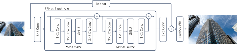
Figure 11: Overall architecture of our $\text{FFNet}{{}_{\textit{sr}}}$ for super-resolution task.

In this section, we explain the architecture of the proposed $\text{FFNet}{{}_{\textit{sr}}}$, adapted for the Super-Resolution (SR) task, as shown in Fig. 11. $\text{FFNet}{{}_{\textit{sr}}}$ consists of three main components: the Shallow Feature Extractor ($H_{SF}$), the Deep Feature Extractor ($H_{DF}$), and the Upscaling Module ($H_{Rec}$).

The shallow feature extractor, $H_{SF}$, serves as the initial stage of the $\text{FFNet}_{\textit{sr}}$ architecture. It utilizes a 3$\times$3 convolution to process the Low-Resolution (LR) input image capturing shallow features. The transformed shallow feature map has a channel size of 96, which is consistent across all variants.

The deep feature extractor, $H_{DF}$, refines the shallow features to produce finer deep features. Each $H_{DF}$ in $\text{FFNet}_{\textit{sr}}$-light and $\text{FFNet}_{\textit{sr}}$ consist of 36 and 48 FFNet Blocks respectively, followed by a final 3$\times$3 convolution. We set the kernel size of all depthwise convolutions to 3 to effectively extract high-frequency details and the expansion ratio of FFN to 2. Importantly, we exclude Batch normalization from the FFNet blocks (see Fig. 3) due to performance degradation, consistent with findings from EDSR [51]. The final 3$\times$3 convolution in $H_{DF}$ reduces the deep feature map’s channels to match those of the long residual skip [115], allowing them to be added element-wise.

We utilize an anchor-based residual skip for the long residual skip, where the input LR image is repeated 4 times along RGB channel-wise [28, 125]. After passing through $H_{Rec}$, the repeated LR image becomes equivalent to a nearest-neighbor interpolated image, enabling the feature extractors to concentrate on recovering high-frequency details.

The upscaling module, $H_{Rec}$, takes the deep features and the long-residual skip, adds them together, and then upscales the result to reconstruct the High-Resolution image. It uses a single PixelShuffle [80] operation, which rearranges the channel dimensions into spatial dimensions in proportion to the upscaling factor. This approach is more efficient and effective than the Transposed Convolution, which often results in checkerboard artifacts [99].

G.3 3D Semantic Segmentation Model Architecture Details

We adopt the serialization-based point cloud preprocessing introduced in PTv3[103] and use a submanifold convolution with 5$\times$5$\times$5 kernel size for embeddings. The encoder and decoder depths are set at [2, 2, 6, 2] and [1, 1, 1, 1], respectively, with channel numbers of [64, 128, 256, 512] for the encoder and [64, 64, 128, 256] for the decoder. The expansion ratio for channel mixer is uniformly set at 4 across all blocks, with GELU as the activation function. Furthermore, we incorporate batch normalization after each submanifold convolution, in addition to the pre-norm, to further stabilize the variance of the feature maps.

G.4 Time Series Forecaster Architecture Details

We introduce two FFN variants tailored for time series data, which maintain the structural integrity of our FFNet block design (Fig. 3 (c)) while effectively computing cross-time and cross-variable interactions. Given the limitations of vanilla FFNs that operate solely along the channel axis, in a multivariate setting with both temporal and variable axes, we propose CVIFFN (Cross-Variable Interaction focused FFN) and CIFFN (Channel Interaction focused FFN) to extract cross-variable dependencies and channel information, respectively. Details of these modules, including PyTorch-like code and intuitive visual explanations, can be found in Algorithm 1, 2, and Fig. 12. Both CVIFFN and CIFFN capture cross-variable and channel information through the first Fully-Connected (FC) layer respectively, then aggregate features across both axes using appropriate group$\&$reshape operations and second FC layer. Thus, our FFNet block for time series replaces the basic block’s FFN with CIFFN and the token mixer’s 1$\times$1 convolution with CVIFFN.

By default, our model includes 1 FFNet block with a hidden dimension of 64 and an expansion ratio of 12. For patch embedding, the patch size and stride are set at 4 and 2, respectively. For the Exchange, ETTh1, and ETTh2 datasets, we reduce the expansion ratio to 2, 2, and 8, respectively, to prevent overfitting. To address distribution shift problem, we utilize RevIN [42]. Finally, for features $O\in\mathbb{R}^{M\times D\times N}$ , we flatten them along the channel $D$ and token $N$ axes, and then compute the final prediction using a linear layer with output channels equal to the prediction length.

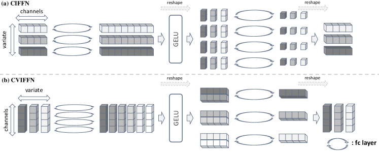
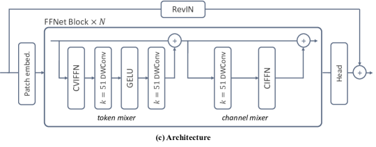
Figure 12: (a-b) Our proposed two types of FFN focus on channel interaction and cross-variable interaction via the first fully-connected layer, respectively. (c) After embedding, stacked FFNet blocks compute cross-time and cross-variable features. Then the final features are fed into the regression head.

Appendix H Training Settings

H.1 3D Semantic Segmentation

We train all models using a grid size of 0.02m, a batch size of 12, and a drop path rate of 0.3. We employ the AdamW optimizer with an initial learning rate of $5\times 10^{-3}$, adjusted via cosine decay, and a weight decay of 0.05. Models are trained for 800 epochs on ScanNet series [17, 77] and 3000 epochs on S3DIS [1] datasets. The data augmentation strategies employed are identical to those used in the PT series [104, 103].

H.2 Long-Term Time Series Forecasting

We train our model with the L2 loss, using Adam optimizer with an initial learning rate of $10^{-4}$. The standard training procedure is 100 epochs, incorporating proper early stopping. Following [57], we fix lookback length 96 for all the datasets and all experiments are repeated three times. We also borrow from the baseline results from iTransformer [57]. Detailed dataset descriptions are summarized in Tab. 11.

Table 11: The overall information of the 8 long-term forecasting datasets.

Dataset	Variable Number	Dataset Size	Sampling Frequency	Information
ETTh (1, 2) [123]	7	(8545, 2881, 2881)	1 hour	Electricity
ETTm (1, 2) [123]	7	(34465, 11521, 11521)	15 mins	Electricity
Exchange [102]	8	(5120, 665, 1422)	1 day	Economy
Weather [102]	21	(36792, 5271, 10540)	10 mins	Weather
ECL [102]	321	(18317, 2633, 5261)	1 hour	Electricity
Traffic [102]	862	(12185, 1757, 3509)	1 hour	Transportation

Algorithm 1 PyTorch-style Code for Cross-Variable Interaction focused FFN

⬇

import torch.nn as nn

class CVIFFN(nn.Module):

"""␣Cross-Variable␣Interaction␣focused␣Feed-Forward␣Network␣"""

def __init__(self, d_model, e_r, n_vars, drop1, drop2):

super().__init__()

d_hidden = d_model * e_r

self.e_r = e_r

self.fc1 = nn.Conv1d(in_channels=n_vars * d_model, out_channels=n_vars * d_hidden, kernel_size=1, stride=1, padding=0, groups=d_model)

self.act = nn.GELU()

self.fc2 = nn.Conv1d(in_channels=n_vars * d_hidden, out_channels=n_vars * d_model, kernel_size=1, stride=1, padding=0, groups=n_vars)

self.drop1 = nn.Dropout(drop1)

self.drop2 = nn.Dropout(drop2)

def forward(self,x):

B, M, D, N = x.shape

x = x.permute(0, 2, 1, 3)

x = x.reshape(B, D * M, N)

x = self.drop1(self.fc1(x))

x = self.act(x)

x = x.reshape(B, D, self.e_r * M, N)

x = x.permute(0, 2, 1, 3)

x = x.reshape(B, M * self.e_r * D, N)

x = self.drop2(self.fc2(x))

x = x.reshape(B, M, D, N)

return x

 

Algorithm 2 PyTorch-style Code for Channel Interaction focused FFN

⬇

import torch.nn as nn

class CIFFN(nn.Module):

"""␣Channel␣Interaction␣focused␣Feed-Forward␣Network␣"""

def __init__(self, d_model, e_r, n_vars, drop1, drop2):

super().__init__()

self.d_hidden = d_model * e_r

self.fc1 = nn.Conv1d(in_channels=n_vars * d_model, out_channels=n_vars * self.d_hidden, kernel_size=1, stride=1, padding=0, groups=n_vars)

self.act = nn.GELU()

self.fc2 = nn.Conv1d(in_channels=n_vars * self.d_hidden, out_channels=n_vars * d_model, kernel_size=1, stride=1, padding=0, groups=d_model)

self.drop1 = nn.Dropout(drop1)

self.drop2 = nn.Dropout(drop2)

def forward(self,x):

B, M, D, N = x.shape

x = x.reshape(B, M * D, N)

x = self.drop1(self.fc1(x))

x = self.act(x)

x = x.reshape(B, M, self.d_hidden, N)

x = x.permute(0, 2, 1, 3)

x = x.reshape(B, self.d_hidden * M, N)

x = self.drop2(self.fc2(x))

x = x.reshape(B, D, M, N)

x = x.permute(0, 2, 1, 3)

return x

 

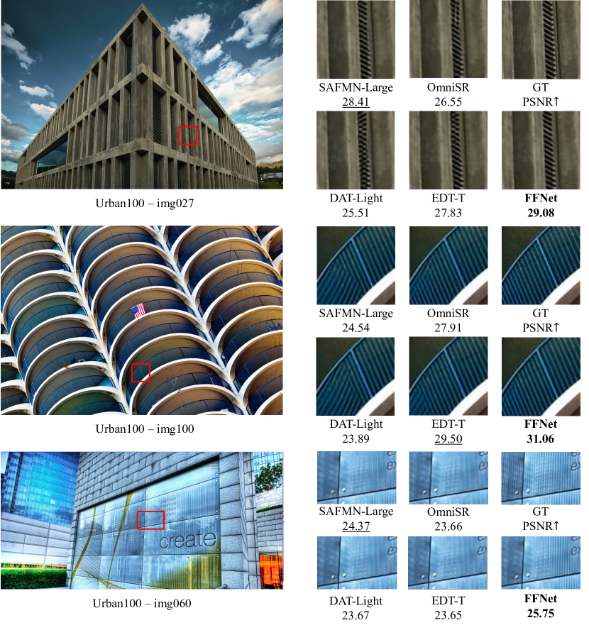
Figure 13: Visual comparison for $\times$2 SR models. The patches for comparison are marked with red boxes. Zoom-in for better visibility.

Appendix I Super-Resolution Visual Results

In this section, we present visual comparisons of our $\text{FFNet}_{\textit{sr}}$ model against state-of-the-art SR models at $\times$2 scale. Figure 13 zooms in on each SR result to emphasize the differences in image sharpness and fine-grained detail preservation, providing corresponding PSNR values. These visualizations underscore the exceptional performance of $\text{FFNet}_{\textit{sr}}$ in the SR task, demonstrating task-generality of the MetaMixer framework.

Appendix J Limitations

While our proposed MetaMixer-based convolutional mixer demonstrates remarkable performance across multiple tasks, showcasing that the MetaMixer itself is crucial rather than specific modules like attention, its effectiveness in more diverse scenarios (such as large-scale datasets like ImageNet-21K or generative modeling requiring flexible conditional operations) remains unproven. Moreover, we acknowledge that our model’s performance is partially improved with the help of recent methods. However, we hope that the new perspectives and possibilities we present will serve as a starting point for future mixer design space and strengthen the systematic approach to model development.

References

- [1] Iro Armeni, Ozan Sener, Amir R Zamir, Helen Jiang, Ioannis Brilakis, Martin Fischer, and Silvio Savarese. 3d semantic parsing of large-scale indoor spaces. In CVPR, 2016.
- [2] Fan Bao, Shen Nie, Kaiwen Xue, Yue Cao, Chongxuan Li, Hang Su, and Jun Zhu. All are worth words: A vit backbone for diffusion models. In CVPR, pages 22669–22679, 2023.
- [3] Marco Bevilacqua, Aline Roumy, Christine Guillemot, and Marie-Line Alberi-Morel. Low-complexity single-image super-resolution based on nonnegative neighbor embedding. In BMVC, 2012.
- [4] Andy Brock, Soham De, Samuel L Smith, and Karen Simonyan. High-performance large-scale image recognition without normalization. In ICML, pages 1059–1071, 2021.
- [5] Han Cai, Junyan Li, Muyan Hu, Chuang Gan, and Song Han. Efficientvit: Lightweight multi-scale attention for high-resolution dense prediction. In ICCV, pages 17302–17313, 2023.
- [6] Zhaowei Cai and Nuno Vasconcelos. Cascade r-cnn: Delving into high quality object detection. In CVPR, 2018.
- [7] Nicolas Carion, Francisco Massa, Gabriel Synnaeve, Nicolas Usunier, Alexander Kirillov, and Sergey Zagoruyko. End-to-end object detection with transformers. In ECCV, pages 213–229. Springer, 2020.
- [8] Kai Chen, Jiaqi Wang, Jiangmiao Pang, Yuhang Cao, Yu Xiong, Xiaoxiao Li, Shuyang Sun, Wansen Feng, Ziwei Liu, Jiarui Xu, Zheng Zhang, Dazhi Cheng, Chenchen Zhu, Tianheng Cheng, Qijie Zhao, Buyu Li, Xin Lu, Rui Zhu, Yue Wu, Jifeng Dai, Jingdong Wang, Jianping Shi, Wanli Ouyang, Chen Change Loy, and Dahua Lin. MMDetection: Open mmlab detection toolbox and benchmark. arXiv preprint arXiv:1906.07155, 2019.
- [9] Yinpeng Chen, Xiyang Dai, Mengchen Liu, Dongdong Chen, Lu Yuan, and Zicheng Liu. Dynamic convolution: Attention over convolution kernels. In CVPR, pages 11030–11039, 2020.
- [10] Yukang Chen, Jianhui Liu, Xiangyu Zhang, Xiaojuan Qi, and Jiaya Jia. Largekernel3d: Scaling up kernels in 3d sparse cnns. In CVPR, 2023.
- [11] Zheng Chen, Yulun Zhang, Jinjin Gu, Linghe Kong, Xiaokang Yang, and Fisher Yu. Dual aggregation transformer for image super-resolution. In ICCV, pages 12312–12321, 2023.
- [12] Bowen Cheng, Alex Schwing, and Alexander Kirillov. Per-pixel classification is not all you need for semantic segmentation. NeurIPS, 2021.
- [13] Haram Choi, Jeongmin Lee, and Jihoon Yang. N-gram in swin transformers for efficient lightweight image super-resolution. In CVPR, pages 2071–2081, 2023.
- [14] MMSegmentation Contributors. MMSegmentation: Openmmlab semantic segmentation toolbox and benchmark. https://github.com/open-mmlab/mmsegmentation, 2020.
- [15] Pointcept Contributors. Pointcept: A codebase for point cloud perception research. https://github.com/Pointcept/Pointcept, 2023.
- [16] Marius Cordts, Mohamed Omran, Sebastian Ramos, Timo Rehfeld, Markus Enzweiler, Rodrigo Benenson, Uwe Franke, Stefan Roth, and Bernt Schiele. The cityscapes dataset for semantic urban scene understanding. In CVPR, pages 3213–3223, 2016.
- [17] Angela Dai, Angel X Chang, Manolis Savva, Maciej Halber, Thomas Funkhouser, and Matthias Nießner. Scannet: Richly-annotated 3d reconstructions of indoor scenes. In CVPR, 2017.
- [18] Damai Dai, Li Dong, Yaru Hao, Zhifang Sui, Baobao Chang, and Furu Wei. Knowledge neurons in pretrained transformers. In ACL, 2022.
- [19] Zihang Dai, Hanxiao Liu, Quoc V Le, and Mingxing Tan. Coatnet: Marrying convolution and attention for all data sizes. NeurIPS, pages 3965–3977, 2021.
- [20] Tri Dao, Dan Fu, Stefano Ermon, Atri Rudra, and Christopher Ré. Flashattention: Fast and memory-efficient exact attention with io-awareness. NeurIPS, pages 16344–16359, 2022.
- [21] Timothée Darcet, Maxime Oquab, Julien Mairal, and Piotr Bojanowski. Vision transformers need registers. In ICLR, 2024.
- [22] Abhimanyu Das, Weihao Kong, Andrew Leach, Rajat Sen, and Rose Yu. Long-term forecasting with tide: Time-series dense encoder. arXiv preprint arXiv:2304.08424, 2023.
- [23] Jia Deng, Wei Dong, Richard Socher, Li-Jia Li, Kai Li, and Li Fei-Fei. Imagenet: A large-scale hierarchical image database. In CVPR, pages 248–255, 2009.
- [24] Xiaohan Ding, Xiangyu Zhang, Jungong Han, and Guiguang Ding. Scaling up your kernels to 31x31: Revisiting large kernel design in cnns. In CVPR, pages 11963–11975, 2022.
- [25] Xiaohan Ding, Xiangyu Zhang, Ningning Ma, Jungong Han, Guiguang Ding, and Jian Sun. Repvgg: Making vgg-style convnets great again. In CVPR, pages 13733–13742, 2021.
- [26] Xiaohan Ding, Yiyuan Zhang, Yixiao Ge, Sijie Zhao, Lin Song, Xiangyu Yue, and Ying Shan. Unireplknet: A universal perception large-kernel convnet for audio, video, point cloud, time-series and image recognition. In CVPR, 2024.
- [27] Alexey Dosovitskiy, Lucas Beyer, Alexander Kolesnikov, Dirk Weissenborn, Xiaohua Zhai, Thomas Unterthiner, Mostafa Dehghani, Matthias Minderer, Georg Heigold, Sylvain Gelly, Jakob Uszkoreit, and Neil Houlsby. An image is worth 16x16 words: Transformers for image recognition at scale. In ICLR, 2021.
- [28] Zongcai Du, Jie Liu, Jie Tang, and Gangshan Wu. Anchor-based plain net for mobile image super-resolution. In CVPR, pages 2494–2502, 2021.
- [29] Kunihiko Fukushima. Visual feature extraction by a multilayered network of analog threshold elements. IEEE Transactions on Systems Science and Cybernetics, 1969.
- [30] Mor Geva, Roei Schuster, Jonathan Berant, and Omer Levy. Transformer feed-forward layers are key-value memories. EMNLP, 2020.
- [31] Benjamin Graham, Martin Engelcke, and Laurens Van Der Maaten. 3d semantic segmentation with submanifold sparse convolutional networks. In CVPR, 2018.
- [32] Jianyuan Guo, Kai Han, Han Wu, Yehui Tang, Xinghao Chen, Yunhe Wang, and Chang Xu. Cmt: Convolutional neural networks meet vision transformers. In CVPR, pages 12175–12185, 2022.
- [33] Meng-Hao Guo, Cheng-Ze Lu, Qibin Hou, Zhengning Liu, Ming-Ming Cheng, and Shi-Min Hu. Segnext: Rethinking convolutional attention design for semantic segmentation. NeurIPS, 2022.
- [34] Kaiming He, Xiangyu Zhang, Shaoqing Ren, and Jian Sun. Deep residual learning for image recognition. In CVPR, pages 770–778, 2016.
- [35] Dan Hendrycks, Steven Basart, Norman Mu, Saurav Kadavath, Frank Wang, Evan Dorundo, Rahul Desai, Tyler Zhu, Samyak Parajuli, Mike Guo, et al. The many faces of robustness: A critical analysis of out-of-distribution generalization. In ICCV, pages 8340–8349, 2021.
- [36] Dan Hendrycks and Kevin Gimpel. Gaussian error linear units (gelus). arXiv preprint arXiv:1606.08415, 2016.
- [37] Dan Hendrycks, Kevin Zhao, Steven Basart, Jacob Steinhardt, and Dawn Song. Natural adversarial examples. In CVPR, pages 15262–15271, 2021.
- [38] Qibin Hou, Li Zhang, Ming-Ming Cheng, and Jiashi Feng. Strip pooling: Rethinking spatial pooling for scene parsing. In CVPR, 2020.
- [39] Jia-Bin Huang, Abhishek Singh, and Narendra Ahuja. Single image super-resolution from transformed self-exemplars. In CVPR, pages 5197–5206, 2015.
- [40] Sergey Ioffe and Christian Szegedy. Batch normalization: Accelerating deep network training by reducing internal covariate shift. In ICML, 2015.
- [41] Jiwon Kim, Jung Kwon Lee, and Kyoung Mu Lee. Accurate image super-resolution using very deep convolutional networks. In CVPR, pages 1646–1654, 2016.
- [42] Taesung Kim, Jinhee Kim, Yunwon Tae, Cheonbok Park, Jang-Ho Choi, and Jaegul Choo. Reversible instance normalization for accurate time-series forecasting against distribution shift. In ICLR, 2022.
- [43] Goro Kobayashi, Tatsuki Kuribayashi, Sho Yokoi, and Kentaro Inui. Analyzing feed-forward blocks in transformers through the lens of attention maps. In ICLR, 2024.
- [44] Alex Krizhevsky, Ilya Sutskever, and Geoffrey E Hinton. Imagenet classification with deep convolutional neural networks. In NeurIPS, 2012.
- [45] Xin Lai, Jianhui Liu, Li Jiang, Liwei Wang, Hengshuang Zhao, Shu Liu, Xiaojuan Qi, and Jiaya Jia. Stratified transformer for 3d point cloud segmentation. In CVPR, 2022.
- [46] Wenbo Li, Xin Lu, Shengju Qian, Jiangbo Lu, Xiangyu Zhang, and Jiaya Jia. On efficient transformer-based image pre-training for low-level vision. arXiv preprint arXiv:2112.10175, 2021.
- [47] Yanyu Li, Ju Hu, Yang Wen, Georgios Evangelidis, Kamyar Salahi, Yanzhi Wang, Sergey Tulyakov, and Jian Ren. Rethinking vision transformers for mobilenet size and speed. In ICCV, pages 16889–16900, 2023.
- [48] Yanyu Li, Geng Yuan, Yang Wen, Ju Hu, Georgios Evangelidis, Sergey Tulyakov, Yanzhi Wang, and Jian Ren. Efficientformer: Vision transformers at mobilenet speed. NeuIPS, pages 12934–12949, 2022.
- [49] Zonglin Li, Chong You, Srinadh Bhojanapalli, Daliang Li, Ankit Singh Rawat, Sashank J Reddi, Ke Ye, Felix Chern, Felix Yu, Ruiqi Guo, et al. The lazy neuron phenomenon: On emergence of activation sparsity in transformers. arXiv preprint arXiv:2210.06313, 2022.
- [50] Jingyun Liang, Jiezhang Cao, Guolei Sun, Kai Zhang, Luc Van Gool, and Radu Timofte. Swinir: Image restoration using swin transformer. In ICCVW, pages 1833–1844, 2021.
- [51] Bee Lim, Sanghyun Son, Heewon Kim, Seungjun Nah, and Kyoung Mu Lee. Enhanced deep residual networks for single image super-resolution. In CVPRW, pages 136–144, 2017.
- [52] Tsung-Yi Lin, Michael Maire, Serge Belongie, James Hays, Pietro Perona, Deva Ramanan, Piotr Dollár, and C Lawrence Zitnick. Microsoft coco: Common objects in context. In ECCV, 2014.
- [53] Minhao Liu, Ailing Zeng, Muxi Chen, Zhijian Xu, Qiuxia Lai, Lingna Ma, and Qiang Xu. Scinet: time series modeling and forecasting with sample convolution and interaction. NeurIPS, 2022.
- [54] Shiwei Liu, Tianlong Chen, Xiaohan Chen, Xuxi Chen, Qiao Xiao, Boqian Wu, Tommi Kärkkäinen, Mykola Pechenizkiy, Decebal Constantin Mocanu, and Zhangyang Wang. More convnets in the 2020s: Scaling up kernels beyond 51x51 using sparsity. In ICLR, 2023.
- [55] Xinyu Liu, Houwen Peng, Ningxin Zheng, Yuqing Yang, Han Hu, and Yixuan Yuan. Efficientvit: Memory efficient vision transformer with cascaded group attention. In CVPR, pages 14420–14430, 2023.
- [56] Yong Liu, Hang Dong, Boyang Liang, Songwei Liu, Qingji Dong, Kai Chen, Fangmin Chen, Lean Fu, and Fei Wang. Unfolding once is enough: A deployment-friendly transformer unit for super-resolution. In MM, pages 7952–7960. ACM, 2023.
- [57] Yong Liu, Tengge Hu, Haoran Zhang, Haixu Wu, Shiyu Wang, Lintao Ma, and Mingsheng Long. itransformer: Inverted transformers are effective for time series forecasting. In ICLR, 2024.
- [58] Yong Liu, Haixu Wu, Jianmin Wang, and Mingsheng Long. Non-stationary transformers: Rethinking the stationarity in time series forecasting. NeurIPS, 2022.
- [59] Ze Liu, Yutong Lin, Yue Cao, Han Hu, Yixuan Wei, Zheng Zhang, Stephen Lin, and Baining Guo. Swin transformer: Hierarchical vision transformer using shifted windows. In ICCV, pages 10012–10022, 2021.
- [60] Zhuang Liu, Hanzi Mao, Chao-Yuan Wu, Christoph Feichtenhofer, Trevor Darrell, and Saining Xie. A convnet for the 2020s. CVPR, 2022.
- [61] Xu Ma, Huan Wang, Can Qin, Kunpeng Li, Xingchen Zhao, Jie Fu, and Yun Fu. A close look at spatial modeling: From attention to convolution. arXiv preprint arXiv:2212.12552, 2022.
- [62] Xu Ma, Huan Wang, Can Qin, Kunpeng Li, Xingchen Zhao, Jie Fu, and Yun Fu. A close look at spatial modeling: From attention to convolution. arXiv preprint arXiv:2212.12552, 2022.
- [63] David Martin, Charless Fowlkes, Doron Tal, and Jitendra Malik. A database of human segmented natural images and its application to evaluating segmentation algorithms and measuring ecological statistics. In ICCV, pages 416–423, 2001.
- [64] Yusuke Matsui, Kota Ito, Yuji Aramaki, Azuma Fujimoto, Toru Ogawa, Toshihiko Yamasaki, and Kiyoharu Aizawa. Sketch-based manga retrieval using manga109 dataset. MM, pages 21811–21838, 2017.
- [65] Sachin Mehta and Mohammad Rastegari. Mobilevit: light-weight, general-purpose, and mobile-friendly vision transformer. In ICLR, 2022.
- [66] Kevin Meng, David Bau, Alex J Andonian, and Yonatan Belinkov. Locating and editing factual associations in GPT. In NeurIPS, 2022.
- [67] Seyed Iman Mirzadeh, Keivan Alizadeh-Vahid, Sachin Mehta, Carlo C del Mundo, Oncel Tuzel, Golnoosh Samei, Mohammad Rastegari, and Mehrdad Farajtabar. ReLU strikes back: Exploiting activation sparsity in large language models. In ICLR, 2024.
- [68] Yuqi Nie, Nam H Nguyen, Phanwadee Sinthong, and Jayant Kalagnanam. A time series is worth 64 words: Long-term forecasting with transformers. ICLR, 2023.
- [69] William Peebles and Saining Xie. Scalable diffusion models with transformers. In ICCV, pages 4195–4205, 2023.
- [70] Bohao Peng, Xiaoyang Wu, Li Jiang, Yukang Chen, Hengshuang Zhao, Zhuotao Tian, and Jiaya Jia. Oa-cnns: Omni-adaptive sparse cnns for 3d semantic segmentation. In CVPR, 2024.
- [71] Chao Peng, Xiangyu Zhang, Gang Yu, Guiming Luo, and Jian Sun. Large kernel matters–improve semantic segmentation by global convolutional network. In CVPR, 2017.
- [72] Guocheng Qian, Yuchen Li, Houwen Peng, Jinjie Mai, Hasan Hammoud, Mohamed Elhoseiny, and Bernard Ghanem. Pointnext: Revisiting pointnet++ with improved training and scaling strategies. NeurIPS, 2022.
- [73] Ilija Radosavovic, Raj Prateek Kosaraju, Ross Girshick, Kaiming He, and Piotr Dollár. Designing network design spaces. In CVPR, 2020.
- [74] Yongming Rao, Wenliang Zhao, Yansong Tang, Jie Zhou, Ser-Lam Lim, and Jiwen Lu. Hornet: Efficient high-order spatial interactions with recursive gated convolutions. NeurIPS, 2022.
- [75] Benjamin Recht, Rebecca Roelofs, Ludwig Schmidt, and Vaishaal Shankar. Do imagenet classifiers generalize to imagenet? In ICML, pages 5389–5400, 2019.
- [76] Olaf Ronneberger, Philipp Fischer, and Thomas Brox. U-net: Convolutional networks for biomedical image segmentation. In MICCAI, pages 234–241, 2015.
- [77] David Rozenberszki, Or Litany, and Angela Dai. Language-grounded indoor 3d semantic segmentation in the wild. In ECCV, 2022.
- [78] Abdelrahman Shaker, Muhammad Maaz, Hanoona Rasheed, Salman Khan, Ming-Hsuan Yang, and Fahad Shahbaz Khan. Swiftformer: Efficient additive attention for transformer-based real-time mobile vision applications. In ICCV, pages 17425–17436, 2023.
- [79] Kai Shen, Junliang Guo, Xu Tan, Siliang Tang, Rui Wang, and Jiang Bian. A study on relu and softmax in transformer. arXiv preprint arXiv:2302.06461, 2023.
- [80] Wenzhe Shi, Jose Caballero, Ferenc Huszár, Johannes Totz, Andrew P Aitken, Rob Bishop, Daniel Rueckert, and Zehan Wang. Real-time single image and video super-resolution using an efficient sub-pixel convolutional neural network. In CVPR, pages 1874–1883, 2016.
- [81] Chenyang Si, Weihao Yu, Pan Zhou, Yichen Zhou, Xinchao Wang, and Shuicheng YAN. Inception transformer. In NeurIPS, 2022.
- [82] Sainbayar Sukhbaatar, Edouard Grave, Guillaume Lample, Herve Jegou, and Armand Joulin. Augmenting self-attention with persistent memory. arXiv preprint arXiv:1907.01470, 2019.
- [83] Sainbayar Sukhbaatar, Jason Weston, Rob Fergus, et al. End-to-end memory networks. NeurIPS, 2015.
- [84] Long Sun, Jiangxin Dong, Jinhui Tang, and Jinshan Pan. Spatially-adaptive feature modulation for efficient image super-resolution. In ICCV, pages 13190–13199, 2023.
- [85] Mingxing Tan and Quoc Le. Efficientnet: Rethinking model scaling for convolutional neural networks. In ICML, pages 6105–6114, 2019.
- [86] Mingxing Tan and Quoc Le. Efficientnetv2: Smaller models and faster training. In ICML, pages 10096–10106, 2021.
- [87] Radu Timofte, Eirikur Agustsson, Luc Van Gool, Ming-Hsuan Yang, and Lei Zhang. Ntire 2017 challenge on single image super-resolution: Methods and results. In CVPRW, pages 114–125, 2017.
- [88] Ilya O Tolstikhin, Neil Houlsby, Alexander Kolesnikov, Lucas Beyer, Xiaohua Zhai, Thomas Unterthiner, Jessica Yung, Andreas Steiner, Daniel Keysers, Jakob Uszkoreit, et al. Mlp-mixer: An all-mlp architecture for vision. NeurIPS, pages 24261–24272, 2021.
- [89] Hugo Touvron, Matthieu Cord, Matthijs Douze, Francisco Massa, Alexandre Sablayrolles, and Hervé Jégou. Training data-efficient image transformers & distillation through attention. In ICML, 2021.
- [90] Hugo Touvron, Matthieu Cord, and Hervé Jégou. Deit iii: Revenge of the vit. In ECCV, pages 516–533, 2022.
- [91] Hugo Touvron, Matthieu Cord, Alexandre Sablayrolles, Gabriel Synnaeve, and Hervé Jégou. Going deeper with image transformers. In ICCV, 2021.
- [92] Zhengzhong Tu, Hossein Talebi, Han Zhang, Feng Yang, Peyman Milanfar, Alan Bovik, and Yinxiao Li. Maxim: Multi-axis mlp for image processing. In CVPR, pages 5769–5780, 2022.
- [93] Pavan Kumar Anasosalu Vasu, James Gabriel, Jeff Zhu, Oncel Tuzel, and Anurag Ranjan. Fastvit: A fast hybrid vision transformer using structural reparameterization. In ICCV, pages 5785–5795, 2023.
- [94] Ashish Vaswani, Noam Shazeer, Niki Parmar, Jakob Uszkoreit, Llion Jones, Aidan N Gomez, Lukasz Kaiser, and Illia Polosukhin. Attention is all you need. In NeurIPS, pages 5998–6008, 2017.
- [95] Hang Wang, Xuanhong Chen, Bingbing Ni, Yutian Liu, and Jinfan Liu. Omni aggregation networks for lightweight image super-resolution. In CVPR, pages 22378–22387, 2023.
- [96] Haohan Wang, Songwei Ge, Zachary Lipton, and Eric P Xing. Learning robust global representations by penalizing local predictive power. NeurIPS, 2019.
- [97] Peng-Shuai Wang. Octformer: Octree-based transformers for 3d point clouds. SIGGRAPH, 2023.
- [98] Xiaozhi Wang, Kaiyue Wen, Zhengyan Zhang, Lei Hou, Zhiyuan Liu, and Juanzi Li. Finding skill neurons in pre-trained transformer-based language models. EMNLP, 2022.
- [99] Yifan Wang, Federico Perazzi, Brian McWilliams, Alexander Sorkine-Hornung, Olga Sorkine-Hornung, and Christopher Schroers. A fully progressive approach to single-image super-resolution. In CVPRW, pages 864–873, 2018.
- [100] Ross Wightman, Hugo Touvron, and Hervé Jégou. Resnet strikes back: An improved training procedure in timm. NeuIPS, 2021.
- [101] Haixu Wu, Tengge Hu, Yong Liu, Hang Zhou, Jianmin Wang, and Mingsheng Long. Timesnet: Temporal 2d-variation modeling for general time series analysis. ICLR, 2023.
- [102] Haixu Wu, Jiehui Xu, Jianmin Wang, and Mingsheng Long. Autoformer: Decomposition transformers with Auto-Correlation for long-term series forecasting. NeurIPS, 2021.
- [103] Xiaoyang Wu, Li Jiang, Peng-Shuai Wang, Zhijian Liu, Xihui Liu, Yu Qiao, Wanli Ouyang, Tong He, and Hengshuang Zhao. Point transformer v3: Simpler, faster, stronger. arXiv preprint arXiv:2312.10035, 2023.
- [104] Xiaoyang Wu, Yixing Lao, Li Jiang, Xihui Liu, and Hengshuang Zhao. Point transformer v2: Grouped vector attention and partition-based pooling. NeurIPS, pages 33330–33342, 2022.
- [105] Tete Xiao, Yingcheng Liu, Bolei Zhou, Yuning Jiang, and Jian Sun. Unified perceptual parsing for scene understanding. In ECCV, 2018.
- [106] Enze Xie, Wenhai Wang, Zhiding Yu, Anima Anandkumar, Jose M Alvarez, and Ping Luo. Segformer: Simple and efficient design for semantic segmentation with transformers. NeurIPS, 2021.
- [107] Chenglin Yang, Siyuan Qiao, Qihang Yu, Xiaoding Yuan, Yukun Zhu, Alan Yuille, Hartwig Adam, and Liang-Chieh Chen. Moat: Alternating mobile convolution and attention brings strong vision models. In ICLR, 2022.
- [108] Jianwei Yang, Chunyuan Li, Xiyang Dai, and Jianfeng Gao. Focal modulation networks. NeurIPS, 2022.
- [109] Yu-Qi Yang, Yu-Xiao Guo, Jian-Yu Xiong, Yang Liu, Hao Pan, Peng-Shuai Wang, Xin Tong, and Baining Guo. Swin3d: A pretrained transformer backbone for 3d indoor scene understanding. arXiv preprint arXiv:2304.06906, 2023.
- [110] Weihao Yu, Mi Luo, Pan Zhou, Chenyang Si, Yichen Zhou, Xinchao Wang, Jiashi Feng, and Shuicheng Yan. Metaformer is actually what you need for vision. CVPR, 2022.
- [111] Seokju Yun and Youngmin Ro. Shvit: Single-head vision transformer with memory efficient macro design. In CVPR, 2024.
- [112] Ailing Zeng, Muxi Chen, Lei Zhang, and Qiang Xu. Are transformers effective for time series forecasting? AAAI, 2023.
- [113] Roman Zeyde, Michael Elad, and Matan Protter. On single image scale-up using sparse-representations. In Curves and Surfaces: 7th International Conference, Avignon, France, June 24-30, 2010, Revised Selected Papers 7, 2012.
- [114] Xindong Zhang, Hui Zeng, Shi Guo, and Lei Zhang. Efficient long-range attention network for image super-resolution. In ECCV, pages 649–667, 2022.
- [115] Yulun Zhang, Kunpeng Li, Kai Li, Lichen Wang, Bineng Zhong, and Yun Fu. Image super-resolution using very deep residual channel attention networks. In ECCV, pages 286–301, 2018.
- [116] Yunhao Zhang and Junchi Yan. Crossformer: Transformer utilizing cross-dimension dependency for multivariate time series forecasting. ICLR, 2023.
- [117] Zhengyan Zhang, Yankai Lin, Zhiyuan Liu, Peng Li, Maosong Sun, and Jie Zhou. Moefication: Transformer feed-forward layers are mixtures of experts. In ACL, 2022.
- [118] Hengshuang Zhao, Jianping Shi, Xiaojuan Qi, Xiaogang Wang, and Jiaya Jia. Pyramid scene parsing network. In CVPR, 2017.
- [119] Yucheng Zhao, Guangting Wang, Chuanxin Tang, Chong Luo, Wenjun Zeng, and Zheng-Jun Zha. A battle of network structures: An empirical study of cnn, transformer, and mlp. arXiv preprint arXiv:2108.13002, 2021.
- [120] Sixiao Zheng, Jiachen Lu, Hengshuang Zhao, Xiatian Zhu, Zekun Luo, Yabiao Wang, Yanwei Fu, Jianfeng Feng, Tao Xiang, Philip HS Torr, et al. Rethinking semantic segmentation from a sequence-to-sequence perspective with transformers. In CVPR, 2021.
- [121] Bolei Zhou, Hang Zhao, Xavier Puig, Sanja Fidler, Adela Barriuso, and Antonio Torralba. Scene parsing through ade20k dataset. In CVPR, pages 633–641, 2017.
- [122] Donghao Zhou, Chunbin Gu, Junde Xu, Furui Liu, Qiong Wang, Guangyong Chen, and Pheng-Ann Heng. Repmode: Learning to re-parameterize diverse experts for subcellular structure prediction. In CVPR, pages 3312–3322, 2023.
- [123] Haoyi Zhou, Shanghang Zhang, Jieqi Peng, Shuai Zhang, Jianxin Li, Hui Xiong, and Wancai Zhang. Informer: Beyond efficient transformer for long sequence time-series forecasting. In AAAI, 2021.
- [124] Tian Zhou, Ziqing Ma, Qingsong Wen, Xue Wang, Liang Sun, and Rong Jin. FEDformer: Frequency enhanced decomposed transformer for long-term series forecasting. ICML, 2022.
- [125] Zhou Zhou, Jiahao Chao, Jiali Gong, Hongfan Gao, Zhenbing Zeng, and Zhengfeng Yang. Enhancing real-time super resolution with partial convolution and efficient variance attention. In MM, pages 5348–5357. ACM, 2023.