On the Mode-Seeking Properties of Langevin Dynamics

Abstract

The Langevin Dynamics framework, which aims to generate samples from the score function of a probability distribution, is widely used for analyzing and interpreting score-based generative modeling. While the convergence behavior of Langevin Dynamics under unimodal distributions has been extensively studied in the literature, in practice the data distribution could consist of multiple distinct modes. In this work, we investigate Langevin Dynamics in producing samples from multimodal distributions and theoretically study its mode-seeking properties. We prove that under a variety of sub-Gaussian mixtures, Langevin Dynamics is unlikely to find all mixture components within a sub-exponential number of steps in the data dimension. To reduce the mode-seeking tendencies of Langevin Dynamics, we propose Chained Langevin Dynamics, which divides the data vector into patches of constant size and generates every patch sequentially conditioned on the previous patches. We perform a theoretical analysis of Chained Langevin Dynamics by reducing it to sampling from a constant-dimensional distribution. We present the results of several numerical experiments on synthetic and real image datasets, supporting our theoretical results on the iteration complexities of sample generation from mixture distributions using the chained and vanilla Langevin Dynamics. The code is available at https://github.com/Xiwei-Cheng/Chained_LD.

1 Introduction

A central task in unsupervised learning involves learning the underlying probability distribution of training data and efficiently generating new samples from the distribution. Score-based generative modeling (SGM) [1] has achieved state-of-the-art performance in various learning tasks including image generation [2, 3, 4, 5, 6, 7], audio synthesis [8, 9], and video generation [10, 11]. In addition to the successful empirical results, the convergence analysis of SGM has attracted significant attention in the recent literature [12, 13, 14, 15, 16].

Stochastic gradient Langevin dynamics (SGLD) [17], as a fundamental methodology to implement and interpret SGM, can produce samples from the (Stein) score function of a probability density, i.e., the gradient of the log probability density function with respect to data. It has been widely recognized that a pitfall of SGLD is its slow mixing rate [18, 19, 20]. Specifically, [2] shows that under a multi-modal data distribution, the samples from Langevin dynamics may have an incorrect relative density across the modes. Based on this finding, [2] proposes anneal Langevin dynamics, which injects different levels of Gaussian noise into the data distribution and samples with SGLD on the perturbed distribution. While outputting the correct relative density across modes can be challenging for SGLD, a natural question is whether SGLD would be able to find all the modes of a multi-modal distribution.

In this work, we study this question by analyzing the mode-seeking properties of SGLD. The notion of mode-seekingness [21, 22, 23, 24] refers to the property that a generative model captures only a subset of the modes of a multi-modal distribution. We note that a similar problem, known as metastability, has been studied in the context of Langevin diffusion, a continuous-time version of SGLD described by stochastic differential equation (SDE) [25, 26, 27]. Specifically, [25] gave a sharp bound on the mean hitting time of Langevin diffusion and proved that it may require exponential (in the space dimensionality $d$) time for transition between modes. Regarding discrete SGLD, [20] constructed a probability distribution whose density is close to a mixture of two well-separated isotropic Gaussians, and proved that SGLD could not find one of the two modes within an exponential number of steps. However, further exploration of mode-seeking tendencies of SGLD and its variants such as annealed Langevin dynamics for general distributions is still lacking in the literature.

In this work, we theoretically formulate and demonstrate the potential mode-seeking tendency of SGLD. We begin by analyzing the convergence under a variety of Gaussian mixture probability distributions, under which SGLD could fail to visit all the mixture components within sub-exponential steps (in the data dimension). Subsequently, we generalize this result to mixture distributions with sub-Gaussian modes. This generalization extends our earlier result on Gaussian mixtures to a significantly larger family of mixture models, as the sub-Gaussian family includes any distribution over an $\ell_{2}$-norm-bounded support set. Furthermore, we extend our theoretical results to anneal Langevin dynamics with bounded noise scales.

To reduce SGLD’s large iteration complexity shown under a high-dimensional input vector, we propose Chained Langevin Dynamics (Chained-LD). Since SGLD could suffer from the curse of dimensionality, we decompose the sample ${\mathbf{x}}\in{\mathbb{R}}^{d}$ into $d/Q$ patches ${\mathbf{x}}^{(1)},\cdots,{\mathbf{x}}^{(d/Q)}$, each of constant size $Q$, and sequentially generate every patch ${\mathbf{x}}^{(q)}$ for all $q\in[d/Q]$ statistically conditioned on previous patches, i.e., $P({\mathbf{x}}^{(q)}\mid{\mathbf{x}}^{(0)},\cdots{\mathbf{x}}^{(q-1)})$. The combination of all patches generated from the conditional distribution faithfully follows the probability density $P({\mathbf{x}})$, while learning each patch requires less cost due to the reduced dimension. We also provide a theoretical analysis of Chained-LD by reducing the convergence of a $d$-dimensional sample to the convergence of each patch.

Finally, we present the results of several numerical experiments to validate our theoretical findings. For synthetic experiments, we consider moderately high-dimensional Gaussian mixture models, where the vanilla and annealed Langevin dynamics could not find all the components within a million steps, while Chained-LD could capture all the components with correct frequencies in ${\mathcal{O}}(10^{4})$ steps. For experiments on real image datasets, we consider a mixture of two modes by using the original images from MNIST/Fashion-MNIST training dataset (black background and white digits/objects) as the first mode and constructing the second mode by i.i.d. flipping the images (white background and black digits/objects) with probability 0.5. Following from [2], we trained a Noise Conditional Score Network (NCSN) to estimate the score function. Our numerical results indicate that vanilla Langevin dynamics can fail to capture the two modes, as also observed by [2]. On the other hand, Chained-LD was capable of finding both modes regardless of initialization. We summarize the contributions of this work as follows:

• Theoretically studying the mode-seeking properties of vanilla and annealed Langevin dynamics,

• Proposing Chained Langevin Dynamics (Chained-LD), which decomposes the sample into patches and sequentially generates each patch conditioned on previous patches,

• Providing a theoretical analysis of the convergence behavior of Chained-LD,

• Numerically comparing the mode-seeking properties of vanilla, annealed, and chained Langevin dynamics.

Notations: We use $[n]$ to denote the set $\left\{{1,2,\cdots,n}\right\}$. Also, in the paper, $\left\|{\cdot}\right\|$ refers to the $\ell_{2}$ norm. We use $\bm{0}_{n}$ and $\bm{1}_{n}$ to denote a 0-vector and 1-vector of length $n$. We use ${\bm{I}}_{n}$ to denote the identity matrix of size $n\times n$. In the text, TV stands for the total variation distance.

2 Related Works

Langevin Dynamics: The convergence guarantees for Langevin diffusion, a continuous version of Langevin dynamics, are classical results extensively studied in the literature [28, 29, 30, 31]. Langevin dynamics, also known as Langevin Monte Carlo, is a discretization of Langevin diffusion typically modeled as a Markov Chain Monte Carlo [17]. For unimodal distributions, e.g., the probability density function that is log-concave or satisfies log-Sobolev inequality, the convergence of Langevin dynamics is provably fast [32, 33, 34]. However, for multimodal distributions, the non-asymptotic convergence analysis is much more challenging [35]. [19] gave an upper bound on the convergence time of Langevin dynamics for arbitrary non-log-concave distributions with certain regularity assumptions, which, however, could be exponentially large without imposing more restrictive assumptions. [20] studied the special case of a mixture of Gaussians of equal variance and provided heuristic analysis of sampling from general non-log-concave distributions.

Mode-Seekingness of Langevin Dynamics: The investigation of the mode-seekingness of generative models starts with different generative adversarial network (GAN) [36] model formulations and divergence measures, from both the practical [37, 38] and theoretical [39, 23, 24] perspectives. In the context of Langevin dynamics, mode-seekingness is closely related to a lower bound on the transition time between two modes, e.g., two local maximums. [25, 26, 27] studied the mean hitting time of the continuous Langevin diffusion. [20] proved the existence of a mixture of two Gaussian distributions whose covariance matrices differ by a constant factor, Langevin dynamics cannot find both modes in polynomial time.

Score-based Generative Modeling: Since [40] proposed sliced score matching which can train deep models to learn the score functions of implicit probability distributions on high-dimensional data, score-based generative modeling (SGM) has been going through a spurt of growth. Annealed Langevin dynamics [2] estimates the noise score of the probability density perturbed by Gaussian noise and utilizes stochastic gradient Langevin dynamics to generate samples from a sequence of decreasing noise scales. [3] conducted a heuristic analysis of the effect of noise levels on the performance of annealed Langevin dynamics. Denoising diffusion probabilistic model (DDPM) [4] incorporates a step-by-step introduction of random noise into data, followed by learning to reverse this diffusion process in order to generate desired data samples from the noise. [1] unified anneal Langevin dynamics and DDPM via a stochastic differential equation. A recent line of work focuses on the non-asymptotic convergence guarantees for SGM with an imperfect score estimation under various assumptions on the data distribution [41, 42, 12, 14, 43, 15, 16].

3 Preliminaries

3.1 Langevin Dynamics

Generative modeling aims to produce samples such that their distribution is close to the underlying true distribution $P$. For a continuously differentiable probability density $P({\mathbf{x}})$ on ${\mathbb{R}}^{d}$, its score function is defined as the gradient of the log probability density function (PDF) $\nabla_{\mathbf{x}}\log P({\mathbf{x}})$. Langevin diffusion is a stochastic process defined by the stochastic differential equation (SDE)

$${\,\mathrm{d}}{\mathbf{x}}_{t}=-\nabla_{\mathbf{x}}\log P({\mathbf{x}}_{t}){\,\mathrm{d}}t+\sqrt{2}{\,\mathrm{d}}{\mathbf{w}}_{t},$$

where ${\mathbf{w}}_{t}$ is the Wiener process on ${\mathbb{R}}^{d}$. To generate samples from Langevin diffusion, [17] proposed stochastic gradient Langevin dynamics (SGLD), a discretization of the SDE for $T$ iterations. Each iteration of SGLD is defined as

$${\mathbf{x}}_{t}={\mathbf{x}}_{t-1}+\frac{\delta_{t}}{2}\nabla_{\mathbf{x}}\log P({\mathbf{x}}_{t-1})+\sqrt{\delta_{t}}\bm{\epsilon}_{t},$$ (1)

where $\delta_{t}$ is the step size and $\bm{\epsilon}_{t}\sim{\mathcal{N}}(\bm{0}_{d},{\bm{I}}_{d})$ is Gaussian noise. It has been widely recognized that Langevin diffusion could take exponential time to mix without additional assumptions on the probability density [25, 26, 27, 19, 20]. To combat the slow mixing, [2] proposed annealed Langevin dynamics by perturbing the probability density with Gaussian noise of variance ${\sigma}^{2}$, i.e.,

$$P_{\sigma}({\mathbf{x}})\mathrel{\mathop{\mathchar 58\relax}}=\int P({\mathbf{z}}){\mathcal{N}}({\mathbf{x}}\mid{\mathbf{z}},{\sigma}^{2}{\bm{I}}_{d}){\,\mathrm{d}}{\mathbf{z}},$$ (2)

and running SGLD on the perturbed data distribution $P_{{\sigma}_{t}}({\mathbf{x}})$ with gradually decreasing noise levels $\left\{{{\sigma}_{t}}\right\}_{t\in[T]}$, i.e.,

$${\mathbf{x}}_{t}={\mathbf{x}}_{t-1}+\frac{\delta_{t}}{2}\nabla_{\mathbf{x}}\log P_{{\sigma}_{t}}({\mathbf{x}}_{t-1})+\sqrt{\delta_{t}}\bm{\epsilon}_{t},$$ (3)

where $\delta_{t}$ is the step size and $\bm{\epsilon}_{t}\sim{\mathcal{N}}(\bm{0}_{d},{\bm{I}}_{d})$ is Gaussian noise. When the noise level ${\sigma}$ is vanishingly small, the perturbed distribution is close to the true distribution, i.e., $P_{\sigma}({\mathbf{x}})\approx P({\mathbf{x}})$. Since we do not have direct access to the (perturbed) score function, [2] proposed the Noise Conditional Score Network (NCSN) ${\mathbf{s}}_{\bm{\theta}}({\mathbf{x}},{\sigma})$ to jointly estimate the scores of all perturbed data distributions, i.e.,

$$\forall{\sigma}\in\left\{{{\sigma}_{t}}\right\}_{t\in[T]},\;{\mathbf{s}}_{\bm{\theta}}({\mathbf{x}},{\sigma})\approx\nabla_{\mathbf{x}}\log P_{{\sigma}}({\mathbf{x}}).$$

To train the NCSN, [2] adopted denoising score matching, which minimizes the following loss

$${\mathcal{L}}\left(\bm{\theta};\left\{{{\sigma}_{t}}\right\}_{t\in[T]}\right)\mathrel{\mathop{\mathchar 58\relax}}=\frac{1}{2T}\sum_{t\in[T]}{\sigma}_{t}^{2}\mathbb{E}_{{\mathbf{x}}\sim P}\mathbb{E}_{\tilde{{\mathbf{x}}}\sim{\mathcal{N}}({\mathbf{x}},{\sigma}_{t}^{2}{\bm{I}}_{d})}\biggl{[}\left\|{{\mathbf{s}}_{\bm{\theta}}(\tilde{{\mathbf{x}}},{\sigma}_{t})-\frac{\tilde{{\mathbf{x}}}-{\mathbf{x}}}{{\sigma}_{t}^{2}}}\right\|^{2}\biggr{]}.$$

Assuming the NCSN has enough capacity, ${\mathbf{s}}_{\bm{\theta}^{*}}({\mathbf{x}},{\sigma})$ minimizes the loss ${\mathcal{L}}\left(\bm{\theta};\left\{{{\sigma}_{t}}\right\}_{t\in[T]}\right)$ if and only if ${\mathbf{s}}_{\bm{\theta}^{*}}({\mathbf{x}},{\sigma}_{t})=\nabla_{\mathbf{x}}\log P_{{\sigma}_{t}}({\mathbf{x}})$ almost surely for all $t\in[T]$.

3.2 Multi-Modal Distributions

Our work focuses on multi-modal distributions. We use $P=\sum_{i\in[k]}w_{i}P^{(i)}$ to represent a mixture of $k$ modes, where each mode $P^{(i)}$ is a probability density with frequency $w_{i}$ such that $w_{i}>0$ for all $i\in[k]$ and $\sum_{i\in[k]}w_{i}=1$. In our theoretical analysis, we consider Gaussian mixtures and sub-Gaussian mixtures, i.e., every component $P^{(i)}$ is a Gaussian or sub-Gaussian distribution. A probability distribution $p({\mathbf{z}})$ of dimension $d$ is defined as a sub-Gaussian distribution with parameter ${\nu}^{2}$ if, given the mean vector ${\bm{\mu}}\mathrel{\mathop{\mathchar 58\relax}}=\mathbb{E}_{{\mathbf{z}}\sim p}[{\mathbf{z}}]$, the moment generating function (MGF) of $p$ satisfies the following inequality for every vector ${\bm{\alpha}}\in{\mathbb{R}}^{d}$:

$$\mathbb{E}_{{\mathbf{z}}\sim p}\left[\exp\left({\bm{\alpha}}^{T}({\mathbf{z}}-{\bm{\mu}}\right)\right]\leq\exp\Bigl{(}\frac{{\nu}^{2}\left\|{{\bm{\alpha}}}\right\|_{2}^{2}}{2}\Bigr{)}.$$ (4)

We remark that sub-Gaussian distributions include a wide variety of distributions such as Gaussian distributions and any distribution within a bounded $\ell_{2}$-norm distance from the mean ${\bm{\mu}}$. From equation 2 we note that the perturbed distribution is the convolution of the original distribution and a Gaussian random variable, i.e., for random variables ${\mathbf{z}}\sim p$ and ${\mathbf{t}}\sim{\mathcal{N}}(\bm{0}_{d},{\bm{I}}_{d})$, their sum ${\mathbf{z}}+{\mathbf{t}}\sim p_{\sigma}$ follows the perturbed distribution with noise level ${\sigma}$. Therefore, a perturbed (sub)Gaussian distribution remains (sub)Gaussian. We formalize this property in Proposition 1 and defer the proof to Appendix A for completeness.

Proposition 1.

Suppose the perturbed distribution of a $d$-dimensional probability distribution $p$ with noise level ${\sigma}$ is $p_{\sigma}$, then the mean of the perturbed distribution is the same as the original distribution, i.e., $\mathbb{E}_{{\mathbf{z}}\sim p_{\sigma}}[{\mathbf{z}}]=\mathbb{E}_{{\mathbf{z}}\sim p}[{\mathbf{z}}]$. If $p={\mathcal{N}}({\bm{\mu}},{\bm{\Sigma}})$ is a Gaussian distribution, $p_{\sigma}={\mathcal{N}}({\bm{\mu}},{\bm{\Sigma}}+{\sigma}^{2}{\bm{I}}_{d})$ is also a Gaussian distribution. If $p$ is a sub-Gaussian distribution with parameter ${\nu}^{2}$, $p_{\sigma}$ is a sub-Gaussian distribution with parameter $({\nu}^{2}+{\sigma}^{2})$.

4 Theoretical Analysis of the Mode-Seeking Properties of Langevin Dynamics

In this section, we theoretically investigate the mode-seeking properties of vanilla and annealed Langevin dynamics. We begin with analyzing Langevin dynamics in Gaussian mixtures.

4.1 Langevin Dynamics in Gaussian Mixtures

Assumption 1.

Consider a data distribution $P\mathrel{\mathop{\mathchar 58\relax}}=\sum_{i=0}^{k}w_{i}P^{(i)}$ as a mixture of Gaussian distributions, where $1\leq k=o(d)$ and $w_{i}>0$ is a positive constant such that $\sum_{i=0}^{k}w_{i}=1$. Suppose that $P^{(i)}={\mathcal{N}}({\bm{\mu}}_{i},{\nu}_{i}^{2}{\bm{I}}_{d})$ is a Gaussian distribution over ${\mathbb{R}}^{d}$ for all $i\in\{0\}\cup[k]$ such that for all $i\in[k]$, ${\nu}_{i}<{\nu}_{0}$ and $\left\|{{\bm{\mu}}_{i}-{\bm{\mu}}_{0}}\right\|^{2}\leq\frac{{\nu}_{0}^{2}-{\nu}_{i}^{2}}{2}\left(\log\left(\frac{{\nu}_{i}^{2}}{{\nu}_{0}^{2}}\right)-\frac{{\nu}_{i}^{2}}{2{\nu}_{0}^{2}}+\frac{{\nu}_{0}^{2}}{2{\nu}_{i}^{2}}\right)d$. Denote ${\nu}_{\max}\mathrel{\mathop{\mathchar 58\relax}}=\max_{i\in[k]}{\nu}_{i}$.

Regarding the first requirement ${\nu}_{i}<{\nu}_{0}$, we first note that the probability density $p({\mathbf{z}})$ of a Gaussian distribution ${\mathcal{N}}({\bm{\mu}},{\nu}^{2}{\bm{I}}_{d})$ decays exponentially in terms of $\frac{\left\|{{\mathbf{z}}-{\bm{\mu}}}\right\|^{2}}{{\nu}^{2}}$. When a state ${\mathbf{z}}$ is sufficiently far from all modes (i.e., $\left\|{{\mathbf{z}}}\right\|\gg\left\|{{\bm{\mu}}_{i}}\right\|$), the Gaussian distribution with the largest variance (i.e., $P^{(0)}$ in Assumption 1) dominates all other modes because $\frac{\left\|{{\mathbf{z}}-{\bm{\mu}}_{0}}\right\|^{2}}{{\nu}_{0}^{2}}\approx\frac{\left\|{{\mathbf{z}}}\right\|^{2}}{{\nu}_{0}^{2}}\gg\frac{\left\|{{\mathbf{z}}}\right\|^{2}}{{\nu}_{i}^{2}}\approx\frac{\left\|{{\mathbf{z}}-{\bm{\mu}}_{i}}\right\|^{2}}{{\nu}_{i}^{2}}$. We call such mode $P^{(0)}$ the universal mode. Therefore, if ${\mathbf{z}}$ is initialized far from all modes, it can only converge to the universal mode because the gradient information of other modes is masked. Once ${\mathbf{z}}$ enters the universal mode $P^{(0)}$, if the step size $\delta_{t}$ of Langevin dynamics is small (i.e., $\delta_{t}\leq{\nu}_{0}^{2}$), it would take exponential steps to escape the local mode $P^{(0)}$; while if the step size is large (i.e., $\delta_{t}>{\nu}_{0}^{2}$), the state ${\mathbf{z}}$ would again be far from all modes and thus the universal mode $P^{(0)}$ dominates all other modes. Hence, ${\mathbf{z}}$ can only visit the universal mode unless the stochastic noise $\bm{\epsilon}_{t}$ miraculously leads it to the region of another mode. In addition, it can be verified that $\log\left(\frac{{\nu}_{i}^{2}}{{\nu}_{0}^{2}}\right)-\frac{{\nu}_{i}^{2}}{2{\nu}_{0}^{2}}+\frac{{\nu}_{0}^{2}}{2{\nu}_{i}^{2}}$ is a positive constant for ${\nu}_{i}<{\nu}_{0}$, thus the second requirement of Assumption 1 essentially represents $\left\|{{\bm{\mu}}_{i}-{\bm{\mu}}_{0}}\right\|^{2}\leq{\mathcal{O}}(d)$. We formalize the intuition in Theorem 1 and defer the proof to Appendix A.1.

Theorem 1.

Consider a data distribution $P$ satisfying Assumption 1. We follow Langevin dynamics for $T=\exp({\mathcal{O}}(d))$ steps. Suppose the sample is initialized in $P^{(0)}$, then with probability at least $1-T\cdot\exp(-\Omega(d))$, we have $\left\|{{\mathbf{x}}_{t}-{\bm{\mu}}_{i}}\right\|^{2}>\frac{{\nu}_{0}^{2}+{\nu}_{\max}^{2}}{2}d$ for all $t\in\{0\}\cup[T]$ and $i\in[k]$.

We note that $\left\|{{\mathbf{x}}_{t}-{\bm{\mu}}_{i}}\right\|^{2}>\frac{{\nu}_{0}^{2}+{\nu}_{\max}^{2}}{2}d$ is a strong notion of mode-seekingness, since the probability density of mode $P^{(i)}={\mathcal{N}}({\bm{\mu}}_{i},{\nu}_{i}^{2}{\bm{I}}_{d})$ concentrates around the $\ell_{2}$-norm ball $\left\{{{\mathbf{z}}\mathrel{\mathop{\mathchar 58\relax}}\left\|{{\mathbf{z}}-{\bm{\mu}}_{i}}\right\|^{2}\leq{\nu}_{i}^{2}d}\right\}$. This notion can also easily be translated into a lower bound in terms of other distance measures such as total variation distance and Wasserstein 2-distance. Moreover, in Theorem 2 we extend the result to annealed Langevin dynamics with bounded noise level, and the proof is deferred to Appendix A.2.

Theorem 2.

Consider a data distribution $P$ satisfying Assumption 1. We follow annealed Langevin dynamics for $T=\exp({\mathcal{O}}(d))$ steps with noise levels $c_{{\sigma}}\geq{\sigma}_{0}\geq\cdots\geq{\sigma}_{T}\geq 0$ for constant $c_{{\sigma}}>0$. In addition, assume for all $i\in[k]$, $\left\|{{\bm{\mu}}_{i}-{\bm{\mu}}_{0}}\right\|^{2}\leq\frac{{\nu}_{0}^{2}-{\nu}_{i}^{2}}{2}\left(\log\left(\frac{{\nu}_{i}^{2}+c_{{\sigma}}^{2}}{{\nu}_{0}^{2}+c_{{\sigma}}^{2}}\right)-\frac{{\nu}_{i}^{2}+c_{{\sigma}}^{2}}{2{\nu}_{0}^{2}+c_{{\sigma}}^{2}}+\frac{{\nu}_{0}^{2}+c_{{\sigma}}^{2}}{2{\nu}_{i}^{2}+c_{{\sigma}}^{2}}\right)d$. Suppose that the sample is initialized in $P^{(0)}_{{\sigma}_{0}}$, then with probability at least $1-T\cdot\exp(-\Omega(d))$, we have $\left\|{{\mathbf{x}}_{t}-{\bm{\mu}}_{i}}\right\|^{2}>\frac{{\nu}_{0}^{2}+{\nu}_{\max}^{2}+2{\sigma}_{t}^{2}}{2}d$ for all $t\in\{0\}\cup[T]$ and $i\in[k]$.

4.2 Langevin Dynamics in Sub-Gaussian Mixtures

We further generalize our results to sub-Gaussian mixtures. We impose the following assumptions on the mixture. It is worth noting that these assumptions automatically hold for Gaussian mixtures.

Assumption 2.

Consider a data distribution $P\mathrel{\mathop{\mathchar 58\relax}}=\sum_{i=0}^{k}w_{i}P^{(i)}$ as a mixture of sub-Gaussian distributions, where $1\leq k=o(d)$ and $w_{i}>0$ is a positive constant such that $\sum_{i=0}^{k}w_{i}=1$. Suppose that $P^{(0)}={\mathcal{N}}({\bm{\mu}}_{0},{\nu}_{0}^{2}{\bm{I}}_{d})$ is Gaussian and for all $i\in[k]$, $P^{(i)}$ satisfies

1. $P^{(i)}$ is a sub-Gaussian distribution of mean ${\bm{\mu}}_{i}$ with parameter ${\nu}_{i}^{2}$,

2. $P^{(i)}$ is differentiable and $\nabla P^{(i)}({\bm{\mu}}_{i})=\bm{0}_{d}$,

3. the score function of $P^{(i)}$ is $L_{i}$-Lipschitz such that $L_{i}\leq\frac{c_{L}}{{\nu}_{i}^{2}}$ for some constant $c_{L}>0$,

4. ${\nu}_{0}^{2}>\max\left\{{1,\frac{4(c_{L}^{2}+c_{{\nu}}c_{L})}{c_{{\nu}}(1-c_{{\nu}})}}\right\}\frac{{\nu}_{\max}^{2}}{1-c_{{\nu}}}$ for constant $c_{{\nu}}\in(0,1)$, where ${\nu}_{\max}\mathrel{\mathop{\mathchar 58\relax}}=\max_{i\in[k]}{\nu}_{i}$,

5. $\left\|{{\bm{\mu}}_{i}-{\bm{\mu}}_{0}}\right\|^{2}\leq\frac{(1-c_{{\nu}}){\nu}_{0}^{2}-{\nu}_{i}^{2}}{2(1-c_{{\nu}})}\left(\log\frac{c_{{\nu}}{\nu}_{i}^{2}}{(c_{L}^{2}+c_{{\nu}}c_{L}){\nu}_{0}^{2}}-\frac{{\nu}_{i}^{2}}{2(1-c_{{\nu}}){\nu}_{0}^{2}}+\frac{(1-c_{{\nu}}){\nu}_{0}^{2}}{2{\nu}_{i}^{2}}\right)d$.

We validate the feasibility of Assumption 2.v. in Lemma 9 in the Appendix. With Assumption 2, we show the mode-seeking tendency of Langevin dynamics under sub-Gaussian distributions in Theorem 3 and defer the proof to Appendix A.3.

Theorem 3.

Consider a data distribution $P$ satisfying Assumption 2. We follow Langevin dynamics for $T=\exp({\mathcal{O}}(d))$ steps. Suppose the sample is initialized in $P^{(0)}$, then with probability at least $1-T\cdot\exp(-{\mathcal{O}}(d))$, we have $\left\|{{\mathbf{x}}_{t}-{\bm{\mu}}_{i}}\right\|^{2}>\left(\frac{{\nu}_{0}^{2}}{2}+\frac{{\nu}_{\max}^{2}}{2(1-c_{{\nu}})}\right)d$ for all $t\in\{0\}\cup[T]$ and $i\in[k]$.

Finally, we slightly modify Assumption 2 and extend our results to annealed Langevin dynamics under sub-Gaussian mixtures in Theorem 4. The details of Assumption 3 and the proof of Theorem 4 are deferred to Appendix A.4.

Theorem 4.

Consider a data distribution $P$ satisfying Assumption 3. We follow annealed Langevin dynamics for $T=\exp({\mathcal{O}}(d))$ steps with noise levels $c_{{\sigma}}\geq{\sigma}_{0}\geq\cdots\geq{\sigma}_{T}\geq 0$. Suppose the sample is initialized in $P^{(0)}_{{\sigma}_{0}}$, then with probability at least $1-T\cdot\exp(-{\mathcal{O}}(d))$, we have $\left\|{{\mathbf{x}}_{t}-{\bm{\mu}}_{i}}\right\|^{2}>\left(\frac{{\nu}_{0}^{2}+{\sigma}_{t}^{2}}{2}+\frac{{\nu}_{\max}^{2}+{\sigma}_{t}^{2}}{2(1-c_{{\nu}})}\right)d$ for all $t\in\{0\}\cup[T]$ and $i\in[k]$.

5 Chained Langevin Dynamics

To reduce the mode-seeking tendencies of vanilla and annealed Langevin dynamics, we propose Chained Langevin Dynamics (Chained-LD) in Algorithm 1. While vanilla and annealed Langevin dynamics apply gradient updates to all coordinates of the sample in every step, we decompose the sample into patches of constant size and generate each patch sequentially to alleviate the exponential dependency on the dimensionality. More precisely, we divide a sample ${\mathbf{x}}$ into $d/Q$ patches ${\mathbf{x}}^{(1)},\cdots{\mathbf{x}}^{(d/Q)}$ of some constant size $Q$, and apply annealed Langevin dynamics to sample each patch ${\mathbf{x}}^{(q)}$ (for $q\in[d/Q]$) from the conditional distribution $P({\mathbf{x}}^{(q)}\mid{\mathbf{x}}^{(1)},\cdots{\mathbf{x}}^{(q-1)})$.

Algorithm 1 Chained Langevin Dynamics (Chained-LD)

1:Patch size $Q$, dimension $d$, conditional score function estimator ${\mathbf{s}}_{\bm{\theta}}$, number of iterations $T$, noise levels $\left\{{{\sigma}_{t}}\right\}_{t\in[TQ/d]}$, step size $\left\{{\delta_{t}}\right\}_{t\in[TQ/d]}$.

2:Initialize ${\mathbf{x}}_{0}$, and divide ${\mathbf{x}}_{0}$ into $d/Q$ patches ${\mathbf{x}}_{0}^{(1)},\cdots{\mathbf{x}}_{0}^{(d/Q)}$ of equal size $Q$

3:for $q\leftarrow 1$ to $d/Q$ do

4:     for $t\leftarrow 1$ to $TQ/d$ do

5:         ${\mathbf{x}}_{t}^{(q)}\leftarrow{\mathbf{x}}_{t-1}^{(q)}+\frac{\delta_{t}}{2}{\mathbf{s}}_{\bm{\theta}}\left({\mathbf{x}}_{t}^{(q)}\mid{\sigma}_{t},{\mathbf{x}}_{t}^{(1)},\cdots,{\mathbf{x}}_{t}^{(q-1)}\right)+\sqrt{\delta_{t}}\bm{\epsilon}_{t}$, where $\bm{\epsilon}_{t}\sim{\mathcal{N}}(\bm{0}_{Q},{\bm{I}}_{Q})$

6:     end for

7:     ${\mathbf{x}}_{0}^{(q)}\leftarrow{\mathbf{x}}_{TQ/d}^{(q)}$

8:end for

9:return ${\mathbf{x}}_{TQ/d}$

An ideal conditional score function estimator ${\mathbf{s}}_{\bm{\theta}}$ could jointly estimate the scores of all perturbed conditional patch distribution, i.e., $\forall{\sigma}\in\left\{{{\sigma}_{t}}\right\}_{t\in[TQ/d]},q\in[d/Q]$,

$${\mathbf{s}}_{\bm{\theta}}\left({\mathbf{x}}^{(q)}\mid{\sigma},{\mathbf{x}}^{(1)},\cdots,{\mathbf{x}}^{(q-1)}\right)\approx\nabla_{{\mathbf{x}}^{(q)}}\log P_{{\sigma}}({\mathbf{x}}^{(q)}\mid{\mathbf{x}}^{(1)},\cdots{\mathbf{x}}^{(q-1)}).$$

Following from [2], we use the denoising score matching to train the estimator. For a given ${\sigma}$, the denoising score matching objective is

$$\ell(\bm{\theta};{\sigma})\mathrel{\mathop{\mathchar 58\relax}}=\frac{1}{2}\mathbb{E}_{{\mathbf{x}}\sim P}\mathbb{E}_{\tilde{{\mathbf{x}}}\sim{\mathcal{N}}({\mathbf{x}},{\sigma}^{2}{\bm{I}}_{d})}\sum_{q\in[d/Q]}\left[\left\|{{\mathbf{s}}_{\bm{\theta}}\left({\mathbf{x}}^{(q)}\mid{\sigma},{\mathbf{x}}^{(1)},\cdots,{\mathbf{x}}^{(q-1)}\right)-\frac{\tilde{{\mathbf{x}}}^{(q)}-{\mathbf{x}}^{(q)}}{{\sigma}^{2}}}\right\|^{2}\right].$$

Then, combining the objectives gives the following loss

$${\mathcal{L}}\left(\bm{\theta};\left\{{{\sigma}_{t}}\right\}_{t\in[TQ/d]}\right)\mathrel{\mathop{\mathchar 58\relax}}=\frac{d}{TQ}\sum_{t\in[TQ/d]}{\sigma}_{t}^{2}\ell(\bm{\theta};{\sigma}_{t}).$$

As shown in [44], an estimator ${\mathbf{s}}_{\bm{\theta}}$ with enough capacity minimizes the loss ${\mathcal{L}}$ if and only if ${\mathbf{s}}_{\bm{\theta}}$ outputs the scores of all perturbed conditional patch distribution almost surely. Ideally, if a sampler perfectly generates every patch, combining all patches gives a sample from the original distribution since $P({\mathbf{x}})=\prod_{q\in[d/Q]}P({\mathbf{x}}^{(q)}\mid{\mathbf{x}}^{(1)},\cdots{\mathbf{x}}^{(q-1)})$. In Theorem 5 we give a linear reduction from producing samples of dimension $d$ using Chained-LD to learning the distribution of a $Q$-dimensional variable for constant $Q$. The proof of Theorem 5 is deferred to Appendix A.5.

Theorem 5.

Consider a sampler algorithm taking the first $q-1$ patches ${\mathbf{x}}^{(1)},\cdots,{\mathbf{x}}^{(q-1)}$ as input and outputing a sample of the next patch ${\mathbf{x}}^{(q)}$ with probability $\hat{P}\left({\mathbf{x}}^{(q)}\mid{\mathbf{x}}^{(1)},\cdots,{\mathbf{x}}^{(q-1)}\right)$ for all $q\in[d/Q]$. Suppose that for every $q\in[d/Q]$ and any given previous patches ${\mathbf{x}}^{(1)},\cdots,{\mathbf{x}}^{(q-1)}$, the sampler algorithm can achieve

$$\text{TV}\left(\hat{P}\left({\mathbf{x}}^{(q)}\mid{\mathbf{x}}^{(1)},\cdots,{\mathbf{x}}^{(q-1)}\right),P\left({\mathbf{x}}^{(q)}\mid{\mathbf{x}}^{(1)},\cdots,{\mathbf{x}}^{(q-1)}\right)\right)\leq\varepsilon\cdot\frac{Q}{d}$$

in $\tau(\varepsilon,d)$ iterations for some $\varepsilon>0$. Then, equipped with the sampler algorithm, the Chained-LD algorithm in $\frac{d}{Q}\cdot\tau(\varepsilon,d)$ iterations can achieve

$$\text{TV}\left(\hat{P}({\mathbf{x}}),P({\mathbf{x}})\right)\leq\varepsilon.$$

6 Numerical Results

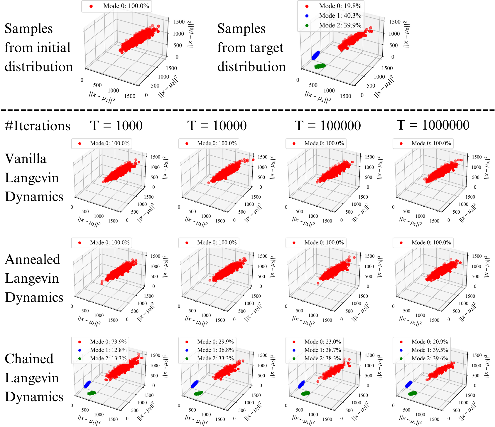
Figure 1: Samples from a mixture of three Gaussian modes generated by vanilla, annealed, and chained Langevin dynamics. Three axes are $\ell_{2}$ distance from samples to the mean of the three modes. The samples are initialized in mode 0.

In this section, we empirically evaluated the mode-seeking tendencies of vanilla, annealed, and chained Langevin dynamics. We performed numerical experiments on synthetic Gaussian mixture models and real image datasets including MNIST [45] and Fashion-MNIST [46]. Details on the experiment setup are deferred to Appendix B.

Synthetic Gaussian mixture model: We define the data distribution $P$ as a mixture of three Gaussian components in dimension $d=100$, where mode 0 defined as $P^{(0)}={\mathcal{N}}(\bm{0}_{d},3{\bm{I}}_{d})$ is the universal mode with the largest variance, and mode 1 and mode 2 are respectively defined as $P^{(1)}={\mathcal{N}}(\bm{1}_{d},{\bm{I}}_{d})$ and $P^{(2)}={\mathcal{N}}(-\bm{1}_{d},{\bm{I}}_{d})$. The frequencies of the three modes are 0.2, 0.4 and 0.4, i.e.,

$$P=0.2P^{(0)}+0.4P^{(1)}+0.4P^{(2)}=0.2{\mathcal{N}}(\bm{0}_{d},3{\bm{I}}_{d})+0.4{\mathcal{N}}(\bm{1}_{d},{\bm{I}}_{d})+0.4{\mathcal{N}}(-\bm{1}_{d},{\bm{I}}_{d}).$$

As shown in Figure 1, vanilla and annealed Langevin dynamics cannot find mode 1 or 2 within $10^{6}$ iterations if the sample is initialized in mode 0, while chained Langevin dynamics can find the other two modes in 1000 steps and correctly recover their frequencies as gradually increasing the number of iterations. In Appendix B.1 we present additional experiments on samples initialized in mode 1 or 2, which also verify the mode-seeking tendencies of vanilla and annealed Langevin dynamics.

Image datasets: We construct the distribution as a mixture of two modes by using the original images from MNIST/Fashion-MNIST training dataset (black background and white digits/objects) as the first mode and constructing the second mode by i.i.d. randomly flipping an image (white background and black digits/objects) with probability 0.5. Regarding the neural network architecture of the score function estimator, for vanilla and annealed Langevin dynamics we use U-Net [47] following from [2]. For chained Langevin dynamics, we proposed to use Recurrent Neural Network (RNN) architectures. We note that for a sequence of inputs, the output of RNN from the previous step is fed as input to the current step. Therefore, in the scenario of chained Langevin dynamics, the hidden state of RNN contains information about the previous patches and allows the network to estimate the conditional score function $\nabla_{{\mathbf{x}}^{(q)}}\log P({\mathbf{x}}^{(q)}\mid{\mathbf{x}}^{(1)},\cdots{\mathbf{x}}^{(q-1)})$. More implementation details are deferred to Appendix B.2.

Figure 2: Samples from a mixture distribution of the original and flipped images from the MNIST dataset generated by vanilla, annealed, and chained Langevin dynamics. The samples are initialized as original images from MNIST.

The numerical results on image datasets are shown in Figures 2 and 3. Vanilla Langevin dynamics fails to generate reasonable samples, as also observed in [2]. When the sample is initialized as original images from the datasets, annealed Langevin dynamics tends to generate samples from the same mode, while chained Langevin dynamics can generate samples from both modes. Additional experiments are deferred to Appendix B.2.

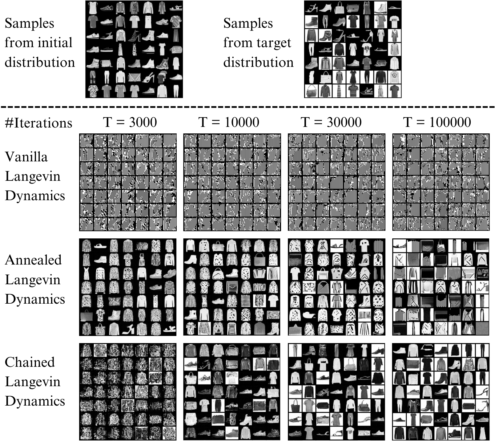
Figure 3: Samples from a mixture distribution of the original and flipped images from the Fashion-MNIST dataset generated by vanilla, annealed, and chained Langevin dynamics. The samples are initialized as original images from Fashion-MNIST.

7 Conclusion

In this work, we theoretically and numerically studied the mode-seeking properties of vanilla and annealed Langevin dynamics sampling methods under a multi-modal distribution. We characterized Gaussian and sub-Gaussian mixture models under which Langevin dynamics are unlikely to find all the components within a sub-exponential number of iterations. To reduce the mode-seeking tendency of vanilla Langevin dynamics, we proposed Chained Langevin Dynamics (Chained-LD) and analyzed its convergence behavior. Studying the connections between Chained-LD and denoising diffusion models will be an interesting topic for future exploration. Our RNN-based implementation of Chained-LD is currently limited to image data generation tasks. An interesting future direction is to extend the application of Chained-LD to other domains such as audio and text data. Another future direction could be to study the convergence of Chained-LD under an imperfect score estimation which we did not address in our analysis.

Appendix A Theoretical Analysis on the Mode-Seeking Tendency of Langevin Dynamics

We begin by introducing some well-established lemmas used in our proof. We first provide the proof of Proposition 1 for completeness:

Proof of Proposition 1.

By the definition in equation 2, we have

$$p_{\sigma}({\mathbf{z}})=\int p({\mathbf{t}}){\mathcal{N}}({\mathbf{z}}\mid{\mathbf{t}},{\sigma}^{2}{\bm{I}}_{d}){\,\mathrm{d}}{\mathbf{t}}=\int p({\mathbf{t}}){\mathcal{N}}({\mathbf{z}}-{\mathbf{t}}\mid\bm{0}_{d},{\sigma}^{2}{\bm{I}}_{d}){\,\mathrm{d}}{\mathbf{t}}.$$

For random variables ${\mathbf{t}}\sim p$ and ${\mathbf{y}}\sim{\mathcal{N}}(\bm{0}_{d},{\bm{I}}_{d})$, their sum ${\mathbf{z}}={\mathbf{t}}+{\mathbf{y}}\sim p_{\sigma}$ follows the perturbed distribution with noise level ${\sigma}$. Therefore,

$$\mathbb{E}_{{\mathbf{z}}\sim p_{\sigma}}[{\mathbf{z}}]=\mathbb{E}_{({\mathbf{t}}+{\mathbf{y}})\sim p_{\sigma}}[{\mathbf{t}}+{\mathbf{y}}]=\mathbb{E}_{{\mathbf{t}}\sim p}[{\mathbf{t}}]+\mathbb{E}_{{\mathbf{y}}\sim{\mathcal{N}}(\bm{0}_{d},{\bm{I}}_{d})}[{\mathbf{y}}]=\mathbb{E}_{{\mathbf{t}}\sim p}[{\mathbf{t}}].$$

If ${\mathbf{t}}\sim p={\mathcal{N}}({\bm{\mu}},{\bm{\Sigma}})$ follows a Gaussian distribution, we have ${\mathbf{z}}={\mathbf{t}}+{\mathbf{y}}\sim p_{\sigma}={\mathcal{N}}({\bm{\mu}},{\bm{\Sigma}}+{\sigma}^{2}{\bm{I}}_{d})$. If $p$ is a sub-Gaussian distribution with parameter ${\nu}^{2}$, we have ${\mathbf{z}}={\mathbf{t}}+{\mathbf{y}}\sim p_{\sigma}$ is a sub-Gaussian distribution with parameter $({\nu}^{2}+{\sigma}^{2})$. Hence we obtain Proposition 1. ∎

We use the following lemma on the tail bound for multivariate Gaussian random variables.

Lemma 1 (Lemma 1, [48]).

Suppose that a random variable ${\mathbf{z}}\sim{\mathcal{N}}(\bm{0}_{d},{\bm{I}}_{d})$. Then for any $\lambda>0$,

$${\mathbb{P}}\left(\left\|{{\mathbf{z}}}\right\|^{2}\geq d+2\sqrt{d\lambda}+2\lambda\right) \leq\exp(-\lambda),$$

$${\mathbb{P}}\left(\left\|{{\mathbf{z}}}\right\|^{2}\leq d-2\sqrt{d\lambda}\right) \leq\exp(-\lambda).$$

We also use a tail bound for one-dimensional Gaussian random variables and provide the proof here for completeness.

Lemma 2.

Suppose a random variable $Z\sim{\mathcal{N}}(0,1)$. Then for any $t>0$,

$${\mathbb{P}}(Z\geq t)={\mathbb{P}}(Z\leq-t)\leq\frac{\exp(-t^{2}/2)}{\sqrt{2\pi}t}.$$

Proof of Lemma 2.

Since $\frac{z}{t}\geq 1$ for all $z\in[t,\infty)$, we have

$${\mathbb{P}}(Z\geq t)=\frac{1}{\sqrt{2\pi}}\int_{t}^{\infty}\exp\left(-\frac{z^{2}}{2}\right){\,\mathrm{d}}z\leq\frac{1}{\sqrt{2\pi}}\int_{t}^{\infty}\frac{z}{t}\exp\left(-\frac{z^{2}}{2}\right){\,\mathrm{d}}z=\frac{\exp(-t^{2}/2)}{\sqrt{2\pi}t}.$$

Since the Gaussian distribution is symmetric, we have ${\mathbb{P}}(Z\geq t)={\mathbb{P}}(Z\leq-t)$. Hence we obtain the desired bound. ∎

A.1 Proof of Theorem 1: Langevin Dynamics under Gaussian Mixtures

Without loss of generality, we assume that ${\bm{\mu}}_{0}=\bm{0}_{d}$ for simplicity. Let $r$ and $n$ respectively denote the rank and nullity of the vector space $\left\{{{\bm{\mu}}_{i}}\right\}_{i\in[k]}$, then we have $r+n=d$ and $0\leq r\leq k=o(d)$. Denote ${\mathbf{R}}\in{\mathbb{R}}^{d\times r}$ an orthonormal basis of the vector space $\left\{{{\bm{\mu}}_{i}}\right\}_{i\in[k]}$, and denote ${\mathbf{N}}\in{\mathbb{R}}^{d\times n}$ an orthonormal basis of the null space of $\left\{{{\bm{\mu}}_{i}}\right\}_{i\in[k]}$. Now consider decomposing the sample ${\mathbf{x}}_{t}$ by

$$\mathbf{r}_{t}\mathrel{\mathop{\mathchar 58\relax}}={\mathbf{R}}^{T}{\mathbf{x}}_{t}\text{, and }\mathbf{n}_{t}\mathrel{\mathop{\mathchar 58\relax}}={\mathbf{N}}^{T}{\mathbf{x}}_{t},$$

where $\mathbf{r}_{t}\in{\mathbb{R}}^{r}$, $\mathbf{n}_{t}\in{\mathbb{R}}^{n}$. Then we have

$${\mathbf{x}}_{t}={\mathbf{R}}\mathbf{r}_{t}+{\mathbf{N}}\mathbf{n}_{t}.$$

Similarly, we decompose the noise $\bm{\epsilon}_{t}$ into

$$\bm{\epsilon}_{t}^{(\mathbf{r})}\mathrel{\mathop{\mathchar 58\relax}}={\mathbf{R}}^{T}\bm{\epsilon}_{t}\text{, and }\bm{\epsilon}_{t}^{(\mathbf{n})}\mathrel{\mathop{\mathchar 58\relax}}={\mathbf{N}}^{T}\bm{\epsilon}_{t},$$

where $\bm{\epsilon}_{t}^{(\mathbf{r})}\in{\mathbb{R}}^{r}$, $\bm{\epsilon}_{t}^{(\mathbf{n})}\in{\mathbb{R}}^{n}$. Then we have

$$\bm{\epsilon}_{t}={\mathbf{R}}\bm{\epsilon}_{t}^{(\mathbf{r})}+{\mathbf{N}}\bm{\epsilon}_{t}^{(\mathbf{n})}.$$

Since a linear combination of a Gaussian random variable still follows Gaussian distribution, by $\bm{\epsilon}_{t}\sim{\mathcal{N}}(\bm{0}_{d},{\bm{I}}_{d})$, ${\mathbf{R}}^{T}{\mathbf{R}}={\bm{I}}_{r}$, and ${\mathbf{N}}^{T}{\mathbf{N}}={\bm{I}}_{n}$ we obtain

$$\bm{\epsilon}_{t}^{(\mathbf{r})}\sim{\mathcal{N}}(\bm{0}_{r},{\bm{I}}_{r})\text{, and }\bm{\epsilon}_{t}^{(\mathbf{n})}\sim{\mathcal{N}}(\bm{0}_{n},{\bm{I}}_{n}).$$

By the definition of Langevin dynamics in equation 1, $\mathbf{n}_{t}$ follow from the update rule:

$$\mathbf{n}_{t} =\mathbf{n}_{t-1}+\frac{\delta_{t}}{2}{\mathbf{N}}^{T}\nabla_{\mathbf{x}}\log P({\mathbf{x}}_{t-1})+\sqrt{\delta_{t}}\bm{\epsilon}_{t}^{(\mathbf{n})}.$$ (5)

It is worth noting that since ${\mathbf{N}}^{T}{\bm{\mu}}_{i}=\bm{0}_{n}$. To show $\left\|{{\mathbf{x}}_{t}-{\bm{\mu}}_{i}}\right\|^{2}>\frac{{\nu}_{0}^{2}+{\nu}_{\max}^{2}}{2}d$, it suffices to prove

$$\left\|{\mathbf{n}_{t}}\right\|^{2}>\frac{{\nu}_{0}^{2}+{\nu}_{\max}^{2}}{2}d.$$

We start by proving that the initialization of the state ${\mathbf{x}}_{0}$ has a large norm on the null space with high probability in the following proposition.

Proposition 2.

Suppose that a sample ${\mathbf{x}}_{0}$ is initialized in the distribution $P^{(0)}$, i.e., ${\mathbf{x}}_{0}\sim P^{(0)}$, then for any constant ${\nu}_{\max}<{\nu}_{0}$, with probability at least $1-\exp(-\Omega(d))$, we have $\left\|{\mathbf{n}_{0}}\right\|^{2}\geq\frac{3{\nu}_{0}^{2}+{\nu}_{\max}^{2}}{4}d$.

Proof of Proposition 2.

Since ${\mathbf{x}}_{0}\sim P^{(0)}={\mathcal{N}}(\bm{0}_{d},{\nu}_{0}^{2}{\bm{I}}_{d})$ and ${\mathbf{N}}^{T}{\mathbf{N}}={\bm{I}}_{n}$, we know $\mathbf{n}_{0}={\mathbf{N}}^{T}{\mathbf{x}}_{0}\sim{\mathcal{N}}(\bm{0}_{n},{\nu}_{0}^{2}{\bm{I}}_{n})$. Therefore, by Lemma 1 we can bound

$${\mathbb{P}}\left(\left\|{\mathbf{n}_{0}}\right\|^{2}\leq\frac{3{\nu}_{0}^{2}+{\nu}_{\max}^{2}}{4}d\right) ={\mathbb{P}}\left(\frac{\left\|{\mathbf{n}_{0}}\right\|^{2}}{{\nu}_{0}^{2}}\leq d-2\sqrt{d\cdot\left(\frac{{\nu}_{0}^{2}-{\nu}_{\max}^{2}}{8{\nu}_{0}^{2}}\right)^{2}d}\right)$$

$$\leq{\mathbb{P}}\left(\frac{\left\|{\mathbf{n}_{0}}\right\|^{2}}{{\nu}_{0}^{2}}\leq n-2\sqrt{n\left(\frac{{\nu}_{0}^{2}-{\nu}_{\max}^{2}}{8{\nu}_{0}^{2}}\right)^{2}\frac{d}{2}}\right)$$

$$\leq\exp\left(-\left(\frac{{\nu}_{0}^{2}-{\nu}_{\max}^{2}}{8{\nu}_{0}^{2}}\right)^{2}\frac{d}{2}\right),$$

where the second last step follows from the assumption $d-n=r=o(d)$. Hence we complete the proof of Proposition 2. ∎

Then, with the assumption that the initialization satisfies $\left\|{\mathbf{n}_{0}}\right\|^{2}\geq\frac{3{\nu}_{0}^{2}+{\nu}_{\max}^{2}}{4}d$, the following proposition shows that $\left\|{\mathbf{n}_{t}}\right\|$ remains large with high probability.

Proposition 3.

Consider a data distribution $P$ satisfies the constraints specified in Theorem 1. We follow the Langevin dynamics for $T=\exp({\mathcal{O}}(d))$ steps. Suppose that the initial sample satisfies $\left\|{\mathbf{n}_{0}}\right\|^{2}\geq\frac{3{\nu}_{0}^{2}+{\nu}_{\max}^{2}}{4}d$, then with probability at least $1-T\cdot\exp(-\Omega(d))$, we have that $\left\|{\mathbf{n}_{t}}\right\|^{2}>\frac{{\nu}_{0}^{2}+{\nu}_{\max}^{2}}{2}d$ for all $t\in\{0\}\cup[T]$.

Proof of Proposition 3.

To establish a lower bound on $\left\|{\mathbf{n}_{t}}\right\|$, we consider different cases of the step size $\delta_{t}$. Intuitively, when $\delta_{t}$ is large enough, $\mathbf{n}_{t}$ will be too noisy due to the introduction of random noise $\sqrt{\delta_{t}}\bm{\epsilon}_{t}^{(\mathbf{n})}$ in equation 5. While for small $\delta_{t}$, the update of $\mathbf{n}_{t}$ is bounded and thus we can iteratively analyze $\mathbf{n}_{t}$. We first handle the case of large $\delta_{t}$ in the following lemma.

Lemma 3.

If $\delta_{t}>{\nu}_{0}^{2}$, with probability at least $1-\exp(-\Omega(d))$, for $\mathbf{n}_{t}$ satisfying equation 5, we have $\left\|{\mathbf{n}_{t}}\right\|^{2}\geq\frac{3{\nu}_{0}^{2}+{\nu}_{\max}^{2}}{4}d$ regardless of the previous state ${\mathbf{x}}_{t-1}$.

Proof of Lemma 3.

Denote ${\mathbf{v}}\mathrel{\mathop{\mathchar 58\relax}}=\mathbf{n}_{t-1}+\frac{\delta_{t}}{2}{\mathbf{N}}^{T}\nabla_{\mathbf{x}}\log P({\mathbf{x}}_{t-1})$ for simplicity. Note that ${\mathbf{v}}$ is fixed for any given ${\mathbf{x}}_{t-1}$. We decompose $\bm{\epsilon}_{t}^{(\mathbf{n})}$ into a vector aligning with ${\mathbf{v}}$ and another vector orthogonal to ${\mathbf{v}}$. Consider an orthonormal matrix ${\mathbf{M}}\in{\mathbb{R}}^{n\times(n-1)}$ such that ${\mathbf{M}}^{T}{\mathbf{v}}=\bm{0}_{n-1}$ and ${\mathbf{M}}^{T}{\mathbf{M}}={\bm{I}}_{n-1}$. By denoting ${\mathbf{u}}\mathrel{\mathop{\mathchar 58\relax}}=\bm{\epsilon}_{t}^{(\mathbf{n})}-{\mathbf{M}}{\mathbf{M}}^{T}\bm{\epsilon}_{t}^{(\mathbf{n})}$ we have ${\mathbf{M}}^{T}{\mathbf{u}}=\bm{0}_{n-1}$, thus we obtain

$$\left\|{\mathbf{n}_{t}}\right\|^{2} =\left\|{{\mathbf{v}}+\sqrt{\delta_{t}}\bm{\epsilon}_{t}^{(\mathbf{n})}}\right\|^{2}$$

$$=\left\|{{\mathbf{v}}+\sqrt{\delta_{t}}{\mathbf{u}}+\sqrt{\delta_{t}}{\mathbf{M}}{\mathbf{M}}^{T}\bm{\epsilon}_{t}^{(\mathbf{n})}}\right\|^{2}$$

$$=\left\|{{\mathbf{v}}+\sqrt{\delta_{t}}{\mathbf{u}}}\right\|^{2}+\left\|{\sqrt{\delta_{t}}{\mathbf{M}}{\mathbf{M}}^{T}\bm{\epsilon}_{t}^{(\mathbf{n})}}\right\|^{2}$$

$$\geq\left\|{\sqrt{\delta_{t}}{\mathbf{M}}{\mathbf{M}}^{T}\bm{\epsilon}_{t}^{(\mathbf{n})}}\right\|^{2}$$

$$\geq{\nu}_{0}^{2}\left\|{{\mathbf{M}}^{T}\bm{\epsilon}_{t}^{(\mathbf{n})}}\right\|^{2}.$$

Since $\bm{\epsilon}_{t}^{(\mathbf{n})}\sim{\mathcal{N}}(\bm{0}_{n},{\bm{I}}_{n})$ and ${\mathbf{M}}^{T}{\mathbf{M}}={\bm{I}}_{n-1}$, we obtain ${\mathbf{M}}^{T}\bm{\epsilon}_{t}^{(\mathbf{n})}\sim{\mathcal{N}}(\bm{0}_{n-1},{\bm{I}}_{n-1})$. Therefore, by Lemma 1 we can bound

$${\mathbb{P}}\left(\left\|{\mathbf{n}_{t}}\right\|^{2}\leq\frac{3{\nu}_{0}^{2}+{\nu}_{\max}^{2}}{4}d\right) \leq{\mathbb{P}}\left(\left\|{{\mathbf{M}}^{T}\bm{\epsilon}_{t}^{(\mathbf{n})}}\right\|^{2}\leq\frac{3{\nu}_{0}^{2}+{\nu}_{\max}^{2}}{4{\nu}_{0}^{2}}d\right)$$

$$={\mathbb{P}}\left(\left\|{{\mathbf{M}}^{T}\bm{\epsilon}_{t}^{(\mathbf{n})}}\right\|^{2}\leq d-2\sqrt{d\cdot\left(\frac{{\nu}_{0}^{2}-{\nu}_{\max}^{2}}{8{\nu}_{0}^{2}}\right)^{2}d}\right)$$

$$\leq{\mathbb{P}}\left(\left\|{{\mathbf{M}}^{T}\bm{\epsilon}_{t}^{(\mathbf{n})}}\right\|^{2}\leq(n-1)-2\sqrt{(n-1)\left(\frac{{\nu}_{0}^{2}-{\nu}_{\max}^{2}}{8{\nu}_{0}^{2}}\right)^{2}\frac{d}{2}}\right)$$

$$\leq\exp\left(-\left(\frac{{\nu}_{0}^{2}-{\nu}_{\max}^{2}}{8{\nu}_{0}^{2}}\right)^{2}\frac{d}{2}\right),$$

where the second last step follows from the assumption $d-n=r=o(d)$. Hence we complete the proof of Lemma 3. ∎

We then consider the case when $\delta_{t}\leq{\nu}_{0}^{2}$. Let $\mathbf{r}\mathrel{\mathop{\mathchar 58\relax}}={\mathbf{R}}^{T}{\mathbf{x}}$ and $\mathbf{n}\mathrel{\mathop{\mathchar 58\relax}}={\mathbf{N}}^{T}{\mathbf{x}}$, then ${\mathbf{x}}={\mathbf{R}}\mathbf{r}+{\mathbf{N}}\mathbf{n}$. We first show that when $\left\|{\mathbf{n}}\right\|^{2}\geq\frac{{\nu}_{0}^{2}+{\nu}_{\max}^{2}}{2}d$, $P^{(i)}({\mathbf{x}})$ is exponentially smaller than $P^{(0)}({\mathbf{x}})$ for all $i\in[k]$ in the following lemma.

Lemma 4.

Given that $\left\|{\mathbf{n}}\right\|^{2}\geq\frac{{\nu}_{0}^{2}+{\nu}_{\max}^{2}}{2}d$ and $\left\|{{\bm{\mu}}_{i}}\right\|^{2}\leq\frac{{\nu}_{0}^{2}-{\nu}_{i}^{2}}{2}\left(\log\left(\frac{{\nu}_{i}^{2}}{{\nu}_{0}^{2}}\right)-\frac{{\nu}_{i}^{2}}{2{\nu}_{0}^{2}}+\frac{{\nu}_{0}^{2}}{2{\nu}_{i}^{2}}\right)d$ for all $i\in[k]$, we have $\frac{P^{(i)}({\mathbf{x}})}{P^{(0)}({\mathbf{x}})}\leq\exp(-\Omega(d))$ for all $i\in[k]$.

Proof of Lemma 4.

For all $i\in[k]$, define $\rho_{i}({\mathbf{x}})\mathrel{\mathop{\mathchar 58\relax}}=\frac{P^{(i)}({\mathbf{x}})}{P^{(0)}({\mathbf{x}})}$, then

$$\rho_{i}({\mathbf{x}}) =\frac{P^{(i)}({\mathbf{x}})}{P^{(0)}({\mathbf{x}})}=\frac{(2\pi{\nu}_{i}^{2})^{-d/2}\exp\left(-\frac{1}{2{\nu}_{i}^{2}}\left\|{{\mathbf{x}}-{\bm{\mu}}_{i}}\right\|^{2}\right)}{(2\pi{\nu}_{0}^{2})^{-d/2}\exp\left(-\frac{1}{2{\nu}_{0}^{2}}\left\|{{\mathbf{x}}}\right\|^{2}\right)}$$

$$=\left(\frac{{\nu}_{0}^{2}}{{\nu}_{i}^{2}}\right)^{d/2}\exp\left(\frac{1}{2{\nu}_{0}^{2}}\left\|{{\mathbf{x}}}\right\|^{2}-\frac{1}{2{\nu}_{i}^{2}}\left\|{{\mathbf{x}}-{\bm{\mu}}_{i}}\right\|^{2}\right)$$

$$=\left(\frac{{\nu}_{0}^{2}}{{\nu}_{i}^{2}}\right)^{d/2}\exp\left(\left(\frac{1}{2{\nu}_{0}^{2}}-\frac{1}{2{\nu}_{i}^{2}}\right)\left\|{{\mathbf{N}}\mathbf{n}}\right\|^{2}+\left(\frac{\left\|{{\mathbf{R}}\mathbf{r}}\right\|^{2}}{2{\nu}_{0}^{2}}-\frac{\left\|{{\mathbf{R}}\mathbf{r}-{\bm{\mu}}_{i}}\right\|^{2}}{2{\nu}_{i}^{2}}\right)\right)$$

$$=\left(\frac{{\nu}_{0}^{2}}{{\nu}_{i}^{2}}\right)^{d/2}\exp\left(\left(\frac{1}{2{\nu}_{0}^{2}}-\frac{1}{2{\nu}_{i}^{2}}\right)\left\|{\mathbf{n}}\right\|^{2}+\left(\frac{\left\|{\mathbf{r}}\right\|^{2}}{2{\nu}_{0}^{2}}-\frac{\left\|{\mathbf{r}-{\mathbf{R}}^{T}{\bm{\mu}}_{i}}\right\|^{2}}{2{\nu}_{i}^{2}}\right)\right),$$

where the last step follows from the definition that ${\mathbf{R}}\in{\mathbb{R}}^{d\times r}$ an orthonormal basis of the vector space $\left\{{{\bm{\mu}}_{i}}\right\}_{i\in[k]}$ and ${\mathbf{N}}^{T}{\mathbf{N}}={\bm{I}}_{n}$. Since ${\nu}_{0}^{2}>{\nu}_{i}^{2}$, the quadratic term $\frac{\left\|{\mathbf{r}}\right\|^{2}}{2{\nu}_{0}^{2}}-\frac{\left\|{\mathbf{r}-{\mathbf{R}}^{T}{\bm{\mu}}_{i}}\right\|^{2}}{2{\nu}_{i}^{2}}$ is maximized at $\mathbf{r}=\frac{{\nu}_{0}^{2}{\mathbf{R}}^{T}{\bm{\mu}}_{i}}{{\nu}_{0}^{2}-{\nu}_{i}^{2}}$. Therefore,

$$\frac{\left\|{\mathbf{r}}\right\|^{2}}{2{\nu}_{0}^{2}}-\frac{\left\|{\mathbf{r}-{\mathbf{R}}^{T}{\bm{\mu}}_{i}}\right\|^{2}}{2{\nu}_{i}^{2}} \leq\frac{{\nu}_{0}^{4}\left\|{{\mathbf{R}}^{T}{\bm{\mu}}_{i}}\right\|^{2}}{2{\nu}_{0}^{2}({\nu}_{0}^{2}-{\nu}_{i}^{2})^{2}}-\frac{1}{2{\nu}_{i}^{2}}\left(\frac{{\nu}_{0}^{2}}{{\nu}_{0}^{2}-{\nu}_{i}^{2}}-1\right)^{2}\left\|{{\mathbf{R}}^{T}{\bm{\mu}}_{i}}\right\|^{2}=\frac{\left\|{{\bm{\mu}}_{i}}\right\|^{2}}{2({\nu}_{0}^{2}-{\nu}_{i}^{2})}.$$

Hence, for $\left\|{\mathbf{n}}\right\|^{2}\geq\frac{{\nu}_{0}^{2}+{\nu}_{\max}^{2}}{2}d$ and $\left\|{{\bm{\mu}}_{i}}\right\|^{2}\leq\frac{{\nu}_{0}^{2}-{\nu}_{i}^{2}}{2}\left(\log\left(\frac{{\nu}_{i}^{2}}{{\nu}_{0}^{2}}\right)-\frac{{\nu}_{i}^{2}}{2{\nu}_{0}^{2}}+\frac{{\nu}_{0}^{2}}{2{\nu}_{i}^{2}}\right)d$, we have

$$\rho_{i}({\mathbf{x}}) =\left(\frac{{\nu}_{0}^{2}}{{\nu}_{i}^{2}}\right)^{d/2}\exp\left(\left(\frac{1}{2{\nu}_{0}^{2}}-\frac{1}{2{\nu}_{i}^{2}}\right)\left\|{\mathbf{n}}\right\|^{2}+\left(\frac{\left\|{\mathbf{r}}\right\|^{2}}{2{\nu}_{0}^{2}}-\frac{\left\|{\mathbf{r}-{\mathbf{R}}^{T}{\bm{\mu}}_{i}}\right\|^{2}}{2{\nu}_{i}^{2}}\right)\right)$$

$$\leq\left(\frac{{\nu}_{0}^{2}}{{\nu}_{i}^{2}}\right)^{d/2}\exp\left(\left(\frac{1}{2{\nu}_{0}^{2}}-\frac{1}{2{\nu}_{i}^{2}}\right)\frac{{\nu}_{0}^{2}+{\nu}_{i}^{2}}{2}d+\frac{\left\|{{\bm{\mu}}_{i}}\right\|^{2}}{2({\nu}_{0}^{2}-{\nu}_{i}^{2})}\right)$$

$$=\exp\left(-\left(\log\left(\frac{{\nu}_{i}^{2}}{{\nu}_{0}^{2}}\right)-\frac{{\nu}_{i}^{2}}{2{\nu}_{0}^{2}}+\frac{{\nu}_{0}^{2}}{2{\nu}_{i}^{2}}\right)\frac{d}{2}+\frac{\left\|{{\bm{\mu}}_{i}}\right\|^{2}}{2({\nu}_{0}^{2}-{\nu}_{i}^{2})}\right)$$

$$\leq\exp\left(-\left(\log\left(\frac{{\nu}_{i}^{2}}{{\nu}_{0}^{2}}\right)-\frac{{\nu}_{i}^{2}}{2{\nu}_{0}^{2}}+\frac{{\nu}_{0}^{2}}{2{\nu}_{i}^{2}}\right)\frac{d}{4}\right).$$

Notice that for function $f(z)=\log z-\frac{z}{2}+\frac{1}{2z}$, we have $f(1)=0$ and $\frac{{\,\mathrm{d}}}{{\,\mathrm{d}}z}f(z)=\frac{1}{z}-\frac{1}{2}-\frac{1}{2z^{2}}=-\frac{1}{2}\left(\frac{1}{z}-1\right)^{2}<0$ when $z\in(0,1)$. Thus, $\log\left(\frac{{\nu}_{i}^{2}}{{\nu}_{0}^{2}}\right)-\frac{{\nu}_{i}^{2}}{2{\nu}_{0}^{2}}+\frac{{\nu}_{0}^{2}}{2{\nu}_{i}^{2}}$ is a positive constant for ${\nu}_{i}<{\nu}_{0}$, i.e., $\rho_{i}({\mathbf{x}})=\exp(-\Omega(d))$. Therefore we finish the proof of Lemma 4. ∎

Lemma 4 implies that when $\left\|{\mathbf{n}}\right\|$ is large, the Gaussian mode $P^{(0)}$ dominates other modes $P^{(i)}$. To bound $\left\|{\mathbf{n}_{t}}\right\|$, we first consider a simpler case that $\left\|{\mathbf{n}_{t-1}}\right\|$ is large. Intuitively, the following lemma proves that when the previous state $\mathbf{n}_{t-1}$ is far from a mode, a single step of Langevin dynamics with bounded step size is not enough to find the mode.

Lemma 5.

Suppose $\delta_{t}\leq{\nu}_{0}^{2}$ and $\left\|{\mathbf{n}_{t-1}}\right\|^{2}>36{\nu}_{0}^{2}d$, then for $\mathbf{n}_{t}$ following from equation 5, we have $\left\|{\mathbf{n}_{t}}\right\|^{2}\geq{\nu}_{0}^{2}d$ with probability at least $1-\exp(-\Omega(d))$.

Proof of Lemma 5.

From the recursion of $\mathbf{n}_{t}$ in equation 5 we have

$$\mathbf{n}_{t} =\mathbf{n}_{t-1}+\frac{\delta_{t}}{2}{\mathbf{N}}^{T}\nabla_{\mathbf{x}}\log P({\mathbf{x}}_{t-1})+\sqrt{\delta_{t}}\bm{\epsilon}_{t}^{(\mathbf{n})}$$

$$=\mathbf{n}_{t-1}-\frac{\delta_{t}}{2}\sum_{i=0}^{k}\frac{P^{(i)}({\mathbf{x}}_{t-1})}{P({\mathbf{x}}_{t-1})}\cdot\frac{{\mathbf{N}}^{T}({\mathbf{x}}_{t-1}-{\bm{\mu}}_{i})}{{\nu}_{i}^{2}}+\sqrt{\delta_{t}}\bm{\epsilon}_{t}^{(\mathbf{n})}$$

$$=\left(1-\frac{\delta_{t}}{2}\sum_{i=0}^{k}\frac{P^{(i)}({\mathbf{x}}_{t-1})}{P({\mathbf{x}}_{t-1})}\cdot\frac{1}{{\nu}_{i}^{2}}\right)\mathbf{n}_{t-1}+\sqrt{\delta_{t}}\bm{\epsilon}_{t}^{(\mathbf{n})}.$$ (6)

By Lemma 4, we have $\frac{P^{(i)}({\mathbf{x}}_{j-1})}{P^{(0)}({\mathbf{x}}_{j-1})}\leq\exp(-\Omega(d))$ for all $i\in[k]$, therefore

$$1-\frac{\delta_{t}}{2}\sum_{i=0}^{k}\frac{P^{(i)}({\mathbf{x}}_{t-1})}{P({\mathbf{x}}_{t-1})}\cdot\frac{1}{{\nu}_{i}^{2}}\geq 1-\frac{\delta_{t}}{2}\cdot\frac{1}{{\nu}_{0}^{2}}-\frac{\delta_{t}}{2}\sum_{i\in[k]}\frac{w_{i}P^{(i)}({\mathbf{x}}_{t-1})}{w_{0}P^{(0)}({\mathbf{x}}_{t-1})}\cdot\frac{1}{{\nu}_{i}^{2}}\geq 1-\frac{1}{2}-\exp(-\Omega(d))>\frac{1}{3}.$$ (7)

On the other hand, from $\bm{\epsilon}_{t}^{(\mathbf{n})}\sim{\mathcal{N}}(\bm{0}_{n},{\bm{I}}_{n})$ we know $\frac{\langle\mathbf{n}_{t-1},\bm{\epsilon}_{t}^{(\mathbf{n})}\rangle}{\left\|{\mathbf{n}_{t-1}}\right\|}\sim{\mathcal{N}}(0,1)$ for any fixed $\mathbf{n}_{t-1}\neq\bm{0}_{n}$, hence by Lemma 2 we have

$${\mathbb{P}}\left(\frac{\langle\mathbf{n}_{t-1},\bm{\epsilon}_{t}^{(\mathbf{n})}\rangle}{\left\|{\mathbf{n}_{t-1}}\right\|}\geq\frac{\sqrt{d}}{4}\right)={\mathbb{P}}\left(\frac{\langle\mathbf{n}_{t-1},\bm{\epsilon}_{t}^{(\mathbf{n})}\rangle}{\left\|{\mathbf{n}_{t-1}}\right\|}\leq-\frac{\sqrt{d}}{4}\right)\leq\frac{4}{\sqrt{2\pi d}}\exp\left(-\frac{d}{32}\right)$$ (8)

Combining equation 6, equation 7 and equation 8 gives that

$$\left\|{\mathbf{n}_{t}}\right\|^{2} \geq\left(\frac{1}{3}\right)^{2}\left\|{\mathbf{n}_{t-1}}\right\|^{2}-2{\nu}_{0}\lvert\langle\mathbf{n}_{t-1},\bm{\epsilon}_{t}^{(\mathbf{n})}\rangle\rvert$$

$$\geq\frac{1}{9}\left\|{\mathbf{n}_{t-1}}\right\|^{2}-\frac{{\nu}_{0}\sqrt{d}}{2}\left\|{\mathbf{n}_{t-1}}\right\|$$

$$\geq\frac{1}{9}\cdot 36{\nu}_{0}^{2}d-\frac{{\nu}_{0}\sqrt{d}}{2}\cdot 6{\nu}_{0}\sqrt{d}$$

$$={\nu}_{0}^{2}d$$

with probability at least $1-\frac{8}{\sqrt{2\pi d}}\exp\left(-\frac{d}{32}\right)=1-\exp(-\Omega(d))$. This proves Lemma 5. ∎

We then proceed to bound $\left\|{\mathbf{n}_{t}}\right\|$ iteratively for $\left\|{\mathbf{n}_{t-1}}\right\|^{2}\leq 36{\nu}_{0}^{2}d$. Recall that equation 5 gives

$$\mathbf{n}_{t}=\mathbf{n}_{t-1}+\frac{\delta_{t}}{2}{\mathbf{N}}^{T}\nabla_{\mathbf{x}}\log P({\mathbf{x}}_{t-1})+\sqrt{\delta_{t}}\bm{\epsilon}_{t}^{(\mathbf{n})}.$$

We notice that the difficulty of solving $\mathbf{n}_{t}$ exhibits in the dependence of $\log P({\mathbf{x}}_{t-1})$ on $\mathbf{r}_{t-1}$. Since $P=\sum_{i=0}^{k}w_{i}P^{(i)}=\sum_{i=0}^{k}w_{i}{\mathcal{N}}({\bm{\mu}}_{i},{\nu}_{i}^{2}{\bm{I}}_{d})$, we can rewrite the score function as

$$\nabla_{\mathbf{x}}\log P({\mathbf{x}}) =\frac{\nabla_{\mathbf{x}}P({\mathbf{x}})}{P({\mathbf{x}})}=-\sum_{i=0}^{k}\frac{P^{(i)}({\mathbf{x}})}{P({\mathbf{x}})}\cdot\frac{{\mathbf{x}}-{\bm{\mu}}_{i}}{{\nu}_{i}^{2}}=-\frac{{\mathbf{x}}}{{\nu}_{0}^{2}}+\sum_{i\in[k]}\frac{P^{(i)}({\mathbf{x}})}{P({\mathbf{x}})}\left(\frac{{\mathbf{x}}}{{\nu}_{0}^{2}}-\frac{{\mathbf{x}}-{\bm{\mu}}_{i}}{{\nu}_{i}^{2}}\right).$$ (9)

Now, instead of directly working with $\mathbf{n}_{t}$, we consider a surrogate recursion $\hat{\mathbf{n}}_{t}$ such that $\hat{\mathbf{n}}_{0}=\mathbf{n}_{0}$ and for all $t\geq 1$,

$$\hat{\mathbf{n}}_{t}=\hat{\mathbf{n}}_{t-1}-\frac{\delta_{t}}{2{\nu}_{0}^{2}}\hat{\mathbf{n}}_{t-1}+\sqrt{\delta_{t}}\bm{\epsilon}_{t}^{(\mathbf{n})}.$$ (10)

The advantage of the surrogate recursion is that $\hat{\mathbf{n}}_{t}$ is independent of $\mathbf{r}$, thus we can obtain the closed-form solution to $\hat{\mathbf{n}}_{t}$. Before we proceed to bound $\hat{\mathbf{n}}_{t}$, we first show that $\hat{\mathbf{n}}_{t}$ is sufficiently close to the original recursion $\mathbf{n}_{t}$ in the following lemma.

Lemma 6.

For any $t\geq 1$, given that $\delta_{j}\leq{\nu}_{0}^{2}$ and $\frac{{\nu}_{0}^{2}+{\nu}_{\max}^{2}}{2}d\leq\left\|{\mathbf{n}_{j-1}}\right\|^{2}\leq 36{\nu}_{0}^{2}d$ for all $j\in[t]$ and $\left\|{{\bm{\mu}}_{i}}\right\|^{2}\leq\frac{{\nu}_{0}^{2}-{\nu}_{i}^{2}}{2}\left(\log\left(\frac{{\nu}_{i}^{2}}{{\nu}_{0}^{2}}\right)-\frac{{\nu}_{i}^{2}}{2{\nu}_{0}^{2}}+\frac{{\nu}_{0}^{2}}{2{\nu}_{i}^{2}}\right)d$ for all $i\in[k]$, we have $\left\|{\hat{\mathbf{n}}_{t}-\mathbf{n}_{t}}\right\|\leq\frac{t}{\exp(\Omega(d))}\sqrt{d}$.

Proof of Lemma 6.

Upon comparing equation 5 and equation 10, by equation 9 we have that for all $j\in[t]$,

$$\left\|{\hat{\mathbf{n}}_{j}-\mathbf{n}_{j}}\right\| =\left\|{\hat{\mathbf{n}}_{j-1}-\frac{\delta_{j}}{2{\nu}_{0}^{2}}\hat{\mathbf{n}}_{j-1}-\mathbf{n}_{j-1}-\frac{\delta_{j}}{2}{\mathbf{N}}^{T}\nabla_{\mathbf{x}}\log P({\mathbf{x}}_{j-1})}\right\|$$

$$=\left\|{\left(1-\frac{\delta_{j}}{2{\nu}_{0}^{2}}\right)(\hat{\mathbf{n}}_{j-1}-\mathbf{n}_{j-1})+\frac{\delta_{j}}{2}\sum_{i\in[k]}\frac{P^{(i)}({\mathbf{x}}_{j-1})}{P({\mathbf{x}}_{j-1})}\left(\frac{1}{{\nu}_{i}^{2}}-\frac{1}{{\nu}_{0}^{2}}\right)\mathbf{n}_{j-1}}\right\|$$

$$\leq\left(1-\frac{\delta_{j}}{2{\nu}_{0}^{2}}\right)\left\|{\hat{\mathbf{n}}_{j-1}-\mathbf{n}_{j-1}}\right\|+\sum_{i\in[k]}\frac{\delta_{j}}{2}\frac{P^{(i)}({\mathbf{x}}_{j-1})}{P({\mathbf{x}}_{j-1})}\left(\frac{1}{{\nu}_{i}^{2}}-\frac{1}{{\nu}_{0}^{2}}\right)\left\|{\mathbf{n}_{j-1}}\right\|$$

$$\leq\left\|{\hat{\mathbf{n}}_{j-1}-\mathbf{n}_{j-1}}\right\|+\sum_{i\in[k]}\frac{\delta_{j}}{2}\frac{P^{(i)}({\mathbf{x}}_{j-1})}{P^{(0)}({\mathbf{x}}_{j-1})}\left(\frac{1}{{\nu}_{i}^{2}}-\frac{1}{{\nu}_{0}^{2}}\right)6{\nu}_{0}\sqrt{d}.$$

By Lemma 4, we have $\frac{P^{(i)}({\mathbf{x}}_{j-1})}{P^{(0)}({\mathbf{x}}_{j-1})}\leq\exp(-\Omega(d))$ for all $i\in[k]$, hence we obtain a recursive bound

$$\left\|{\hat{\mathbf{n}}_{j}-\mathbf{n}_{j}}\right\|\leq\left\|{\hat{\mathbf{n}}_{j-1}-\mathbf{n}_{j-1}}\right\|+\frac{1}{\exp(\Omega(d))}\sqrt{d}.$$

Finally, by $\hat{\mathbf{n}}_{0}=\mathbf{n}_{0}$, we have

$$\left\|{\hat{\mathbf{n}}_{t}-\mathbf{n}_{t}}\right\|=\sum_{j\in[t]}\left(\left\|{\hat{\mathbf{n}}_{j}-\mathbf{n}_{j}}\right\|-\left\|{\hat{\mathbf{n}}_{j-1}-\mathbf{n}_{j-1}}\right\|\right)\leq\frac{t}{\exp(\Omega(d))}\sqrt{d}.$$

Hence we obtain Lemma 6. ∎

We then proceed to analyze $\hat{\mathbf{n}}_{t}$, The following lemma gives us the closed-form solution of $\hat{\mathbf{n}}_{t}$. We slightly abuse the notations here, e.g., $\prod_{i=c_{1}}^{c_{2}}\left(1-\frac{\delta_{i}}{2{\nu}_{0}^{2}}\right)=1$ and $\sum_{j=c_{1}}^{c_{2}}\delta_{j}=0$ for $c_{1}>c_{2}$.

Lemma 7.

For all $t\geq 0$, $\hat{\mathbf{n}}_{t}\sim{\mathcal{N}}\left(\prod_{i=1}^{t}\left(1-\frac{\delta_{i}}{2{\nu}_{0}^{2}}\right)\mathbf{n}_{0},\;\sum_{j=1}^{t}\prod_{i=j+1}^{t}\left(1-\frac{\delta_{i}}{2{\nu}_{0}^{2}}\right)^{2}\delta_{j}{\bm{I}}_{n}\right)$, where the mean and covariance satisfy $\prod_{i=1}^{t}\left(1-\frac{\delta_{i}}{2{\nu}_{0}^{2}}\right)^{2}+\frac{1}{{\nu}_{0}^{2}}\sum_{j=1}^{t}\prod_{i=j+1}^{t}\left(1-\frac{\delta_{i}}{2{\nu}_{0}^{2}}\right)^{2}\delta_{j}\geq 1$.

Proof of Lemma 7.

We prove the two properties by induction. When $t=0$, they are trivial. Suppose they hold for $t-1$, then for the distribution of $\hat{\mathbf{n}}_{t}$, we have

$$\hat{\mathbf{n}}_{t} =\hat{\mathbf{n}}_{t-1}-\frac{\delta_{t}}{2{\nu}_{0}^{2}}\hat{\mathbf{n}}_{t-1}+\sqrt{\delta_{t}}\bm{\epsilon}_{t}^{(\mathbf{n})}$$

$$\sim{\mathcal{N}}\left(\left(1-\frac{\delta_{t}}{2{\nu}_{0}^{2}}\right)\prod_{i=1}^{t-1}\left(1-\frac{\delta_{i}}{2{\nu}_{0}^{2}}\right)\mathbf{n}_{0},\;\left(1-\frac{\delta_{t}}{2{\nu}_{0}^{2}}\right)^{2}\sum_{j=1}^{t-1}\prod_{i=j+1}^{t-1}\left(1-\frac{\delta_{i}}{2{\nu}_{0}^{2}}\right)^{2}\delta_{j}{\bm{I}}_{n}+\delta_{t}{\bm{I}}_{n}\right)$$

$$={\mathcal{N}}\left(\prod_{i=1}^{t}\left(1-\frac{\delta_{i}}{2{\nu}_{0}^{2}}\right)\mathbf{n}_{0},\;\sum_{j=1}^{t}\prod_{i=j+1}^{t}\left(1-\frac{\delta_{i}}{2{\nu}_{0}^{2}}\right)^{2}\delta_{j}{\bm{I}}_{n}\right).$$

For the second property,

$$\quad\prod_{i=1}^{t}\left(1-\frac{\delta_{i}}{2{\nu}_{0}^{2}}\right)^{2}+\frac{1}{{\nu}_{0}^{2}}\sum_{j=1}^{t}\prod_{i=j+1}^{t}\left(1-\frac{\delta_{i}}{2{\nu}_{0}^{2}}\right)^{2}\delta_{j}$$

$$=\left(1-\frac{\delta_{t}}{2{\nu}_{0}^{2}}\right)^{2}\left(\prod_{i=1}^{t-1}\left(1-\frac{\delta_{i}}{2{\nu}_{0}^{2}}\right)^{2}+\frac{1}{{\nu}_{0}^{2}}\sum_{j=1}^{t-1}\prod_{i=j+1}^{t-1}\left(1-\frac{\delta_{i}}{2{\nu}_{0}^{2}}\right)^{2}\delta_{j}\right)+\frac{1}{{\nu}_{0}^{2}}\delta_{t}$$

$$\geq\left(1-\frac{\delta_{t}}{2{\nu}_{0}^{2}}\right)^{2}+\frac{1}{{\nu}_{0}^{2}}\delta_{t}=1+\frac{\delta_{t}^{2}}{4{\nu}_{0}^{4}}\geq 1.$$

Hence we finish the proof of Lemma 7. ∎

Armed with Lemma 7, we are now ready to establish the lower bound on $\left\|{\hat{\mathbf{n}}_{t}}\right\|$. For simplicity, denote $\alpha\mathrel{\mathop{\mathchar 58\relax}}=\prod_{i=1}^{t}\left(1-\frac{\delta_{i}}{2{\nu}_{0}^{2}}\right)^{2}$ and $\beta\mathrel{\mathop{\mathchar 58\relax}}=\frac{1}{{\nu}_{0}^{2}}\sum_{j=1}^{t}\prod_{i=j+1}^{t}\left(1-\frac{\delta_{i}}{2{\nu}_{0}^{2}}\right)^{2}\delta_{j}$. By Lemma 7 we know $\hat{\mathbf{n}}_{t}\sim{\mathcal{N}}(\alpha\mathbf{n}_{0},\beta{\nu}_{0}^{2}{\bm{I}}_{n})$, so we can write $\hat{\mathbf{n}}_{t}=\alpha\mathbf{n}_{0}+\sqrt{\beta}{\nu}_{0}\bm{\epsilon}$, where $\bm{\epsilon}\sim{\mathcal{N}}(\bm{0}_{n},{\bm{I}}_{n})$.

Lemma 8.

Given that $\left\|{\hat{\mathbf{n}}_{0}}\right\|^{2}\geq\frac{3{\nu}_{0}^{2}+{\nu}_{\max}^{2}}{4}d$, we have $\left\|{\hat{\mathbf{n}}_{t}}\right\|^{2}\geq\frac{5{\nu}_{0}^{2}+3{\nu}_{\max}^{2}}{8}d$ with probability at least $1-\exp\left(-\Omega(d)\right)$.

Proof of Lemma 8.

By $\hat{\mathbf{n}}_{t}=\alpha\mathbf{n}_{0}+\sqrt{\beta}{\nu}_{0}\bm{\epsilon}$ we have

$$\left\|{\hat{\mathbf{n}}_{t}}\right\|^{2}=\alpha^{2}\left\|{\mathbf{n}_{0}}\right\|^{2}+\beta{\nu}_{0}^{2}\left\|{\bm{\epsilon}}\right\|^{2}+2\alpha\sqrt{\beta}{\nu}_{0}\langle\mathbf{n}_{0},\bm{\epsilon}\rangle$$

By Lemma 1 we can bound

$${\mathbb{P}}\left(\left\|{\bm{\epsilon}}\right\|^{2}\leq\frac{3{\nu}_{0}^{2}+{\nu}_{\max}^{2}}{4{\nu}_{0}^{2}}d\right) ={\mathbb{P}}\left(\left\|{\bm{\epsilon}}\right\|^{2}\leq d-2\sqrt{d\cdot\left(\frac{{\nu}_{0}^{2}-{\nu}_{\max}^{2}}{8{\nu}_{0}^{2}}\right)^{2}d}\right)$$

$$\leq{\mathbb{P}}\left(\left\|{\bm{\epsilon}}\right\|^{2}\leq(n-1)-2\sqrt{(n-1)\left(\frac{{\nu}_{0}^{2}-{\nu}_{\max}^{2}}{8{\nu}_{0}^{2}}\right)^{2}\frac{d}{2}}\right)$$

$$\leq\exp\left(-\left(\frac{{\nu}_{0}^{2}-{\nu}_{\max}^{2}}{8{\nu}_{0}^{2}}\right)^{2}\frac{d}{2}\right),$$

where the second last step follows from the assumption $d-n=r=o(d)$. Since $\bm{\epsilon}\sim{\mathcal{N}}(\bm{0}_{n},{\bm{I}}_{n})$, we know $\frac{\langle\mathbf{n}_{0},\bm{\epsilon}\rangle}{\left\|{\mathbf{n}_{0}}\right\|}\sim{\mathcal{N}}(0,1)$. Therefore by Lemma 2,

$${\mathbb{P}}\left(\frac{\langle\mathbf{n}_{0},\bm{\epsilon}\rangle}{\left\|{\mathbf{n}_{0}}\right\|}\leq-\frac{{\nu}_{0}^{2}-{\nu}_{\max}^{2}}{4{\nu}_{0}\sqrt{3{\nu}_{0}^{2}+{\nu}_{\max}^{2}}}\sqrt{d}\right)\leq\frac{4{\nu}_{0}\sqrt{3{\nu}_{0}^{2}+{\nu}_{\max}^{2}}}{\sqrt{2\pi}({\nu}_{0}^{2}-{\nu}_{\max}^{2})\sqrt{d}}\exp\left(-\frac{({\nu}_{0}^{2}-{\nu}_{\max}^{2})^{2}d}{32{\nu}_{0}^{2}(3{\nu}_{0}^{2}+{\nu}_{\max}^{2})}\right)$$

Conditioned on $\left\|{\hat{\mathbf{n}}_{0}}\right\|^{2}\geq\frac{3{\nu}_{0}^{2}+{\nu}_{\max}^{2}}{4}d$, $\left\|{\bm{\epsilon}}\right\|^{2}>\frac{3{\nu}_{0}^{2}+{\nu}_{\max}^{2}}{4{\nu}_{0}^{2}}d$ and $\frac{1}{\left\|{\mathbf{n}_{0}}\right\|}\langle\mathbf{n}_{0},\bm{\epsilon}\rangle>-\frac{{\nu}_{0}^{2}-{\nu}_{\max}^{2}}{4{\nu}_{0}\sqrt{3{\nu}_{0}^{2}+{\nu}_{\max}^{2}}}\sqrt{d}$, since Lemma 7 gives $\alpha^{2}+\beta\geq 1$ we have

$$\left\|{\hat{\mathbf{n}}_{t}}\right\|^{2} =\alpha^{2}\left\|{\mathbf{n}_{0}}\right\|^{2}+\beta{\nu}_{0}^{2}\left\|{\bm{\epsilon}}\right\|^{2}+2\alpha\sqrt{\beta}{\nu}_{0}\langle\mathbf{n}_{0},\bm{\epsilon}\rangle$$

$$\geq\alpha^{2}\left\|{\mathbf{n}_{0}}\right\|^{2}+\beta{\nu}_{0}^{2}\left\|{\bm{\epsilon}}\right\|^{2}-2\alpha\sqrt{\beta}{\nu}_{0}\left\|{\mathbf{n}_{0}}\right\|\frac{{\nu}_{0}^{2}-{\nu}_{\max}^{2}}{4{\nu}_{0}\sqrt{3{\nu}_{0}^{2}+{\nu}_{\max}^{2}}}\sqrt{d}$$

$$\geq\alpha^{2}\left\|{\mathbf{n}_{0}}\right\|^{2}+\beta{\nu}_{0}^{2}\left\|{\bm{\epsilon}}\right\|^{2}-2\alpha\sqrt{\beta}{\nu}_{0}\left\|{\mathbf{n}_{0}}\right\|\left\|{\bm{\epsilon}}\right\|\cdot\frac{{\nu}_{0}^{2}-{\nu}_{\max}^{2}}{6{\nu}_{0}^{2}+2{\nu}_{\max}^{2}}$$

$$\geq\left(1-\frac{{\nu}_{0}^{2}-{\nu}_{\max}^{2}}{6{\nu}_{0}^{2}+2{\nu}_{\max}^{2}}\right)\left(\alpha^{2}\left\|{\mathbf{n}_{0}}\right\|^{2}+\beta{\nu}_{0}^{2}\left\|{\bm{\epsilon}}\right\|^{2}\right)$$

$$\geq\frac{5{\nu}_{0}^{2}+3{\nu}_{\max}^{2}}{6{\nu}_{0}^{2}+2{\nu}_{\max}^{2}}\left(\alpha^{2}+\beta\right)\cdot\frac{3{\nu}_{0}^{2}+{\nu}_{\max}^{2}}{4}d$$

$$\geq\frac{5{\nu}_{0}^{2}+3{\nu}_{\max}^{2}}{8}d.$$

Hence by union bound, we complete the proof of Lemma 8. ∎

Upon having all the above lemmas, we are now ready to establish Proposition 3 by induction. Suppose the theorem holds for all $T$ values of $1,\cdots,T-1$. We consider the following 3 cases:

• If there exists some $t\in[T]$ such that $\delta_{t}>{\nu}_{0}^{2}$, by Lemma 3 we know that with probability at least $1-\exp(-\Omega(d))$, we have $\left\|{\mathbf{n}_{t}}\right\|^{2}\geq\frac{3{\nu}_{0}^{2}+{\nu}_{\max}^{2}}{4}d$, thus the problem reduces to the two sub-arrays $\mathbf{n}_{0},\cdots,\mathbf{n}_{t-1}$ and $\mathbf{n}_{t},\cdots,\mathbf{n}_{T}$, which can be solved by induction.

• Suppose $\delta_{t}\leq{\nu}_{0}^{2}$ for all $t\in[T]$. If there exists some $t\in[T]$ such that $\left\|{\mathbf{n}_{t-1}}\right\|^{2}>36{\nu}_{0}^{2}d$, by Lemma 5 we know that with probability at least $1-\exp(-\Omega(d))$, we have $\left\|{\mathbf{n}_{t}}\right\|^{2}\geq{\nu}_{0}^{2}d>\frac{3{\nu}_{0}^{2}+{\nu}_{\max}^{2}}{4}d$, thus the problem similarly reduces to the two sub-arrays $\mathbf{n}_{0},\cdots,\mathbf{n}_{t-1}$ and $\mathbf{n}_{t},\cdots,\mathbf{n}_{T}$, which can be solved by induction.

• Suppose $\delta_{t}\leq{\nu}_{0}^{2}$ and $\left\|{\mathbf{n}_{t-1}}\right\|^{2}\leq 36{\nu}_{0}^{2}d$ for all $t\in[T]$. Conditioned on $\left\|{\mathbf{n}_{t-1}}\right\|^{2}>\frac{{\nu}_{0}^{2}+{\nu}_{\max}^{2}}{2}d$ for all $t\in[T]$, by Lemma 6 we have that for $T=\exp({\mathcal{O}}(d))$,

  $$\left\|{\hat{\mathbf{n}}_{T}-\mathbf{n}_{T}}\right\|<\left(\sqrt{\frac{5{\nu}_{0}^{2}+3{\nu}_{\max}^{2}}{8}}-\sqrt{\frac{{\nu}_{0}^{2}+{\nu}_{\max}^{2}}{2}}\right)\sqrt{d}.$$

  By Lemma 8 we have that with probability at least $1-\exp(-\Omega(d))$,

  $$\left\|{\hat{\mathbf{n}}_{T}}\right\|^{2}\geq\frac{5{\nu}_{0}^{2}+3{\nu}_{\max}^{2}}{8}d.$$

  Combining the two inequalities implies the desired bound

  $$\left\|{\mathbf{n}_{T}}\right\|\geq\left\|{\hat{\mathbf{n}}_{T}}\right\|-\left\|{\hat{\mathbf{n}}_{T}-\mathbf{n}_{T}}\right\|>\sqrt{\frac{{\nu}_{0}^{2}+{\nu}_{\max}^{2}}{2}d}.$$

  Hence by induction we obtain $\left\|{\mathbf{n}_{t}}\right\|^{2}>\frac{{\nu}_{0}^{2}+{\nu}_{\max}^{2}}{2}d$ for all $t\in[T]$ with probability at least

  $$(1-(T-1)\exp(-\Omega(d)))\cdot(1-\exp(-\Omega(d)))\geq 1-T\exp(-\Omega(d)).$$

Therefore we complete the proof of Proposition 3. ∎

Finally, combining Propositions 2 and 3 finishes the proof of Theorem 1.

A.2 Proof of Theorem 2: Annealed Langevin Dynamics under Gaussian Mixtures

To establish Theorem 2, we first note from Proposition 1 that perturbing a Gaussian distribution ${\mathcal{N}}({\bm{\mu}},{\nu}^{2}{\bm{I}}_{d})$ with noise level ${\sigma}$ results in a Gaussian distribution ${\mathcal{N}}({\bm{\mu}},({\nu}^{2}+{\sigma}^{2}){\bm{I}}_{d})$. Therefore, for a Gaussian mixture $P=\sum_{i=0}^{k}w_{i}P^{(i)}=\sum_{i=0}^{k}w_{i}{\mathcal{N}}({\bm{\mu}}_{i},{\nu}_{i}^{2}{\bm{I}}_{d})$, the perturbed distribution of noise level ${\sigma}$ is

$$P_{\sigma}=\sum_{i=0}^{k}w_{i}{\mathcal{N}}({\bm{\mu}}_{i},({\nu}_{i}^{2}+{\sigma}^{2}){\bm{I}}_{d}).$$

Similar to the proof of Theorem 1, we decompose

$${\mathbf{x}}_{t}={\mathbf{R}}\mathbf{r}_{t}+{\mathbf{N}}\mathbf{n}_{t}\text{, and }\bm{\epsilon}_{t}={\mathbf{R}}\bm{\epsilon}_{t}^{(\mathbf{r})}+{\mathbf{N}}\bm{\epsilon}_{t}^{(\mathbf{n})},$$

where ${\mathbf{R}}\in{\mathbb{R}}^{d\times r}$ an orthonormal basis of the vector space $\left\{{{\bm{\mu}}_{i}}\right\}_{i\in[k]}$ and ${\mathbf{N}}\in{\mathbb{R}}^{d\times n}$ an orthonormal basis of the null space of $\left\{{{\bm{\mu}}_{i}}\right\}_{i\in[k]}$. Now, we prove Theorem 2 by applying the techniques developed in Appendix A.1 via substituting ${\nu}^{2}$ with ${\nu}^{2}+{\sigma}_{t}^{2}$ at time step $t$.

First, by Proposition 2, suppose that the sample is initialized in the distribution $P^{(0)}_{{\sigma}_{0}}$, then with probability at least $1-\exp(-\Omega(d))$, we have

$$\left\|{\mathbf{n}_{0}}\right\|^{2}\geq\frac{3({\nu}_{0}^{2}+{\sigma}_{0}^{2})+({\nu}_{\max}^{2}+{\sigma}_{0}^{2})}{4}d=\frac{3{\nu}_{0}^{2}+{\nu}_{\max}^{2}+4{\sigma}_{0}^{2}}{4}d.$$ (11)

Then, with the assumption that the initialization satisfies $\left\|{\mathbf{n}_{0}}\right\|^{2}\geq\frac{3{\nu}_{0}^{2}+{\nu}_{\max}^{2}+4{\sigma}_{0}^{2}}{4}d$, the following proposition similar to Proposition 3 shows that $\left\|{\mathbf{n}_{t}}\right\|$ remains large with high probability.

Proposition 4.

Consider a data distribution $P$ satisfies the constraints specified in Theorem 2. We follow annealed Langevin dynamics for $T=\exp({\mathcal{O}}(d))$ steps with noise level $c_{{\sigma}}\geq{\sigma}_{0}\geq{\sigma}_{1}\geq{\sigma}_{2}\geq\cdots\geq{\sigma}_{T}\geq 0$ for some constant $c_{{\sigma}}>0$. Suppose that the initial sample satisfies $\left\|{\mathbf{n}_{0}}\right\|^{2}\geq\frac{3{\nu}_{0}^{2}+{\nu}_{\max}^{2}+4{\sigma}_{0}^{2}}{4}d$, then with probability at least $1-T\cdot\exp(-\Omega(d))$, we have that $\left\|{\mathbf{n}_{t}}\right\|^{2}>\frac{{\nu}_{0}^{2}+{\nu}_{\max}^{2}+2{\sigma}_{t}^{2}}{2}d$ for all $t\in\{0\}\cup[T]$.

Proof of Proposition 4.

We prove Proposition 4 by induction. Suppose the theorem holds for all $T$ values of $1,\cdots,T-1$. We consider the following 3 cases:

• If there exists some $t\in[T]$ such that $\delta_{t}>{\nu}_{0}^{2}+{\sigma}_{t}^{2}$, by Lemma 3 we know that with probability at least $1-\exp(-\Omega(d))$, we have $\left\|{\mathbf{n}_{t}}\right\|^{2}\geq\frac{3({\nu}_{0}^{2}+{\sigma}_{t}^{2})+({\nu}_{\max}^{2}+{\sigma}_{t}^{2})}{4}d=\frac{3{\nu}_{0}^{2}+{\nu}_{\max}^{2}+4{\sigma}_{t}^{2}}{4}d$, thus the problem reduces to the two sub-arrays $\mathbf{n}_{0},\cdots,\mathbf{n}_{t-1}$ and $\mathbf{n}_{t},\cdots,\mathbf{n}_{T}$, which can be solved by induction.

• Suppose $\delta_{t}\leq{\nu}_{0}^{2}+{\sigma}_{t}^{2}$ for all $t\in[T]$. If there exists some $t\in[T]$ such that $\left\|{\mathbf{n}_{t-1}}\right\|^{2}>36({\nu}_{0}^{2}+{\sigma}_{t-1}^{2})d\geq 36({\nu}_{0}^{2}+{\sigma}_{t}^{2})d$, by Lemma 5 we know that with probability at least $1-\exp(-\Omega(d))$, we have $\left\|{\mathbf{n}_{t}}\right\|^{2}\geq({\nu}_{0}^{2}+{\sigma}_{t}^{2})d>\frac{3{\nu}_{0}^{2}+{\nu}_{\max}^{2}+4{\sigma}_{t}^{2}}{4}d$, thus the problem similarly reduces to the two sub-arrays $\mathbf{n}_{0},\cdots,\mathbf{n}_{t-1}$ and $\mathbf{n}_{t},\cdots,\mathbf{n}_{T}$, which can be solved by induction.

• Suppose $\delta_{t}\leq{\nu}_{0}^{2}+{\sigma}_{t}^{2}$ and $\left\|{\mathbf{n}_{t-1}}\right\|^{2}\leq 36({\nu}_{0}^{2}+{\sigma}_{t-1}^{2})d$ for all $t\in[T]$. Consider a surrogate sequence $\hat{\mathbf{n}}_{t}$ such that $\hat{\mathbf{n}}_{0}=\mathbf{n}_{0}$ and for all $t\geq 1$,

  $$\hat{\mathbf{n}}_{t}=\hat{\mathbf{n}}_{t-1}-\frac{\delta_{t}}{2{\nu}_{0}^{2}+2{\sigma}_{t}^{2}}\hat{\mathbf{n}}_{t-1}+\sqrt{\delta_{t}}\bm{\epsilon}_{t}^{(\mathbf{n})}.$$

  Since ${\nu}_{0}>{\nu}_{i}$ and $c_{{\sigma}}\geq{\sigma}_{t}$ for all $t\in\left\{{0}\right\}\cup[T]$, we have $\frac{{\nu}_{i}^{2}+c_{{\sigma}}^{2}}{{\nu}_{0}^{2}+c_{{\sigma}}^{2}}\geq\frac{{\nu}_{i}^{2}+{\sigma}_{t}^{2}}{{\nu}_{0}^{2}+{\sigma}_{t}^{2}}$. Notice that for function $f(z)=\log z-\frac{z}{2}+\frac{1}{2z}$, we have $\frac{{\,\mathrm{d}}}{{\,\mathrm{d}}z}f(z)=\frac{1}{z}-\frac{1}{2}-\frac{1}{2z^{2}}=-\frac{1}{2}\left(\frac{1}{z}-1\right)^{2}\leq 0$. Thus, by the assumption

  $$\left\|{{\bm{\mu}}_{i}-{\bm{\mu}}_{0}}\right\|^{2}\leq\frac{{\nu}_{0}^{2}-{\nu}_{i}^{2}}{2}\left(\log\left(\frac{{\nu}_{i}^{2}+c_{{\sigma}}^{2}}{{\nu}_{0}^{2}+c_{{\sigma}}^{2}}\right)-\frac{{\nu}_{i}^{2}+c_{{\sigma}}^{2}}{2{\nu}_{0}^{2}+c_{{\sigma}}^{2}}+\frac{{\nu}_{0}^{2}+c_{{\sigma}}^{2}}{2{\nu}_{i}^{2}+c_{{\sigma}}^{2}}\right)d,$$

  we have that for all $t\in[T]$,

  $$\left\|{{\bm{\mu}}_{i}-{\bm{\mu}}_{0}}\right\|^{2}\leq\frac{{\nu}_{0}^{2}-{\nu}_{i}^{2}}{2}\left(\log\left(\frac{{\nu}_{i}^{2}+{\sigma}_{t}^{2}}{{\nu}_{0}^{2}+{\sigma}_{t}^{2}}\right)-\frac{{\nu}_{i}^{2}+{\sigma}_{t}^{2}}{2{\nu}_{0}^{2}+{\sigma}_{t}^{2}}+\frac{{\nu}_{0}^{2}+{\sigma}_{t}^{2}}{2{\nu}_{i}^{2}+{\sigma}_{t}^{2}}\right)d.$$

  Conditioned on $\left\|{\mathbf{n}_{t-1}}\right\|^{2}>\frac{{\nu}_{0}^{2}+{\nu}_{\max}^{2}+2{\sigma}_{t-1}^{2}}{2}d$ for all $t\in[T]$, by Lemma 6 we have that for $T=\exp({\mathcal{O}}(d))$,

  $$\left\|{\hat{\mathbf{n}}_{T}-\mathbf{n}_{T}}\right\|<\left(\sqrt{\frac{5{\nu}_{0}^{2}+3{\nu}_{\max}^{2}+8{\sigma}_{T}^{2}}{8}}-\sqrt{\frac{{\nu}_{0}^{2}+{\nu}_{\max}^{2}+2{\sigma}_{T}^{2}}{2}}\right)\sqrt{d}.$$

  By Lemma 8 we have that with probability at least $1-\exp(-\Omega(d))$,

  $$\left\|{\hat{\mathbf{n}}_{T}}\right\|^{2}\geq\frac{5{\nu}_{0}^{2}+3{\nu}_{\max}^{2}+8{\sigma}_{T}^{2}}{8}d.$$

  Combining the two inequalities implies the desired bound

  $$\left\|{\mathbf{n}_{T}}\right\|\geq\left\|{\hat{\mathbf{n}}_{T}}\right\|-\left\|{\hat{\mathbf{n}}_{T}-\mathbf{n}_{T}}\right\|>\sqrt{\frac{{\nu}_{0}^{2}+{\nu}_{\max}^{2}+2{\sigma}_{T}^{2}}{2}d}.$$

  Hence by induction we obtain $\left\|{\mathbf{n}_{t}}\right\|^{2}>\frac{{\nu}_{0}^{2}+{\nu}_{\max}^{2}+2{\sigma}_{t}^{2}}{2}d$ for all $t\in\left\{{0}\right\}\cup[T]$ with probability at least

  $$(1-(T-1)\exp(-\Omega(d)))\cdot(1-\exp(-\Omega(d)))\geq 1-T\exp(-\Omega(d)).$$

Therefore we complete the proof of Proposition 4. ∎

Finally, combining equation 11 and Proposition 4 finishes the proof of Theorem 2.

A.3 Proof of Theorem 3: Langevin Dynamics under Sub-Gaussian Mixtures

The proof framework is similar to the proof of Theorem 1. To begin with, we validate Assumption 2.v. in the following lemma:

Lemma 9.

For constants ${\nu}_{0},{\nu}_{i},c_{{\nu}},c_{L}$ satisfying Assumptions 2.iii. and 2.iv., we have $\frac{(1-c_{{\nu}}){\nu}_{0}^{2}-{\nu}_{i}^{2}}{2(1-c_{{\nu}})}>0$ and $\log\frac{c_{{\nu}}{\nu}_{i}^{2}}{(c_{L}^{2}+c_{{\nu}}c_{L}){\nu}_{0}^{2}}-\frac{{\nu}_{i}^{2}}{2(1-c_{{\nu}}){\nu}_{0}^{2}}+\frac{(1-c_{{\nu}}){\nu}_{0}^{2}}{2{\nu}_{i}^{2}}>0$ are both positive constants.

Proof of Lemma 9.

From Assumption 2.iv. that ${\nu}_{0}^{2}>\frac{{\nu}_{\max}^{2}}{1-c_{{\nu}}}\geq\frac{{\nu}_{i}^{2}}{1-c_{{\nu}}}$, we easily obtain $\frac{(1-c_{{\nu}}){\nu}_{0}^{2}-{\nu}_{i}^{2}}{2(1-c_{{\nu}})}>0$ is a positive constant. For the second property, let $f(z)\mathrel{\mathop{\mathchar 58\relax}}=\log\frac{c_{{\nu}}{\nu}_{i}^{2}}{(c_{L}^{2}+c_{{\nu}}c_{L})z}-\frac{{\nu}_{i}^{2}}{2(1-c_{{\nu}})z}+\frac{(1-c_{{\nu}})z}{2{\nu}_{i}^{2}}$. For any $z>\frac{{\nu}_{i}^{2}}{1-c_{{\nu}}}$, the derivative of $f(z)$ satisfies

$$\frac{{\,\mathrm{d}}}{{\,\mathrm{d}}z}f(z)=-\frac{1}{z}+\frac{{\nu}_{i}^{2}}{2(1-c_{{\nu}})z^{2}}+\frac{1-c_{{\nu}}}{2{\nu}_{i}^{2}}=\frac{{\nu}_{i}^{2}}{2(1-c_{{\nu}})}\left(\frac{1-c_{{\nu}}}{{\nu}_{i}^{2}}-\frac{1}{z}\right)^{2}>0.$$

Therefore, when $\frac{4(c_{L}^{2}+c_{{\nu}}c_{L})}{c_{{\nu}}(1-c_{{\nu}})}\leq 1$, we have

$$f({\nu}_{0}^{2})>f\left(\frac{{\nu}_{i}^{2}}{1-c_{{\nu}}}\right)=\log\frac{c_{{\nu}}(1-c_{{\nu}})}{c_{L}^{2}+c_{{\nu}}c_{L}}\geq\log 4>0.$$

When $\frac{4(c_{L}^{2}+c_{{\nu}}c_{L})}{c_{{\nu}}(1-c_{{\nu}})}>1$, we have

$$f({\nu}_{0}^{2}) >f\left(\frac{4(c_{L}^{2}+c_{{\nu}}c_{L})}{c_{{\nu}}(1-c_{{\nu}})}\frac{{\nu}_{i}^{2}}{1-c_{{\nu}}}\right)=2\log\frac{c_{{\nu}}(1-c_{{\nu}})}{2(c_{L}^{2}+c_{{\nu}}c_{L})}-\frac{c_{{\nu}}(1-c_{{\nu}})}{8(c_{L}^{2}+c_{{\nu}}c_{L})}+\frac{2(c_{L}^{2}+c_{{\nu}}c_{L})}{c_{{\nu}}(1-c_{{\nu}})}$$

$$\geq 2-2\log 2-\frac{2(c_{L}^{2}+c_{{\nu}}c_{L})}{c_{{\nu}}(1-c_{{\nu}})}-\frac{c_{{\nu}}(1-c_{{\nu}})}{8(c_{L}^{2}+c_{{\nu}}c_{L})}+\frac{2(c_{L}^{2}+c_{{\nu}}c_{L})}{c_{{\nu}}(1-c_{{\nu}})}>2-2\log 2-\frac{1}{2}>0.$$

Thus we obtain Lemma 9. ∎

Without loss of generality, we assume ${\bm{\mu}}_{0}=\bm{0}_{d}$. Similar to the proof of Theorem 1, we decompose

$${\mathbf{x}}_{t}={\mathbf{R}}\mathbf{r}_{t}+{\mathbf{N}}\mathbf{n}_{t}\text{, and }\bm{\epsilon}_{t}={\mathbf{R}}\bm{\epsilon}_{t}^{(\mathbf{r})}+{\mathbf{N}}\bm{\epsilon}_{t}^{(\mathbf{n})},$$

where ${\mathbf{R}}\in{\mathbb{R}}^{d\times r}$ an orthonormal basis of the vector space $\left\{{{\bm{\mu}}_{i}}\right\}_{i\in[k]}$ and ${\mathbf{N}}\in{\mathbb{R}}^{d\times n}$ an orthonormal basis of the null space of $\left\{{{\bm{\mu}}_{i}}\right\}_{i\in[k]}$. To show $\left\|{{\mathbf{x}}_{t}-{\bm{\mu}}_{i}}\right\|^{2}>\left(\frac{{\nu}_{0}^{2}}{2}+\frac{{\nu}_{\max}^{2}}{2(1-c_{{\nu}})}\right)d$, it suffices to prove $\left\|{\mathbf{n}_{t}}\right\|^{2}>\left(\frac{{\nu}_{0}^{2}}{2}+\frac{{\nu}_{\max}^{2}}{2(1-c_{{\nu}})}\right)d$. By Proposition 2, if ${\mathbf{x}}_{0}$ is initialized in the distribution $P^{(0)}$, i.e., ${\mathbf{x}}_{0}\sim P^{(0)}$, since ${\nu}_{0}^{2}>\frac{1}{1-c_{{\nu}}}{\nu}_{\max}^{2}$, with probability at least $1-\exp(-\Omega(d))$ we have

$$\left\|{\mathbf{n}_{0}}\right\|^{2}\geq\left(\frac{3{\nu}_{0}^{2}}{4}+\frac{{\nu}_{\max}^{2}}{4(1-c_{{\nu}})}\right)d.$$ (12)

Then, conditioned on $\left\|{\mathbf{n}_{0}}\right\|^{2}\geq\left(\frac{3{\nu}_{0}^{2}}{4}+\frac{{\nu}_{\max}^{2}}{4(1-c_{{\nu}})}\right)d$, the following proposition shows that $\left\|{\mathbf{n}_{t}}\right\|$ remains large with high probability.

Proposition 5.

Consider a distribution $P$ satisfying Assumption 2. We follow the Langevin dynamics for $T=\exp({\mathcal{O}}(d))$ steps. Suppose that the initial sample satisfies $\left\|{\mathbf{n}_{0}}\right\|^{2}\geq\left(\frac{3{\nu}_{0}^{2}}{4}+\frac{{\nu}_{\max}^{2}}{4(1-c_{{\nu}})}\right)d$, then with probability at least $1-T\cdot\exp(-\Omega(d))$, we have that $\left\|{\mathbf{n}_{t}}\right\|^{2}>\left(\frac{{\nu}_{0}^{2}}{2}+\frac{{\nu}_{\max}^{2}}{2(1-c_{{\nu}})}\right)d$ for all $t\in\{0\}\cup[T]$.

Proof of Proposition 5.

Firstly, by Lemma 3, if $\delta_{t}>{\nu}_{0}^{2}$, since ${\nu}_{0}^{2}>\frac{{\nu}_{\max}^{2}}{1-c_{{\nu}}}$, we similarly have that $\left\|{\mathbf{n}_{t}}\right\|^{2}\geq\left(\frac{3{\nu}_{0}^{2}}{4}+\frac{{\nu}_{\max}^{2}}{4(1-c_{{\nu}})}\right)d$ with probability at least $1-\exp(-\Omega(d))$ regardless of the previous state ${\mathbf{x}}_{t-1}$. We then consider the case when $\delta_{t}\leq{\nu}_{0}^{2}$. Intuitively, we aim to prove that the score function is close to $-\frac{{\mathbf{x}}}{{\nu}_{0}^{2}}$ when $\left\|{\mathbf{n}}\right\|^{2}\geq\left(\frac{{\nu}_{0}^{2}}{2}+\frac{{\nu}_{\max}^{2}}{2(1-c_{{\nu}})}\right)d$. Towards this goal, we first show that $P^{(0)}({\mathbf{x}})$ is exponentially larger than $P^{(i)}({\mathbf{x}})$ for all $i\in[k]$ in the following lemma:

Lemma 10.

Suppose $P$ satisfies Assumption 2. Then for any $\left\|{\mathbf{n}}\right\|^{2}\geq\left(\frac{{\nu}_{0}^{2}}{2}+\frac{{\nu}_{\max}^{2}}{2(1-c_{{\nu}})}\right)d$, we have $\frac{P^{(i)}({\mathbf{x}})}{P^{(0)}({\mathbf{x}})}\leq\exp(-\Omega(d))$ and $\frac{\left\|{\nabla_{\mathbf{x}}P^{(i)}({\mathbf{x}})}\right\|}{P({\mathbf{x}})}\leq\exp(-\Omega(d))$ for all $i\in[k]$.

Proof of Lemma 10.

We first give an upper bound on the sub-Gaussian probability density. For any vector ${\mathbf{v}}\in{\mathbb{R}}^{d}$, by considering some vector ${\mathbf{m}}\in{\mathbb{R}}^{d}$, from Markov’s inequality and the definition in equation 4 we can bound

$${\mathbb{P}}_{{\mathbf{z}}\sim P^{(i)}}\left({\mathbf{m}}^{T}({\mathbf{z}}-{\bm{\mu}}_{i})\geq{\mathbf{m}}^{T}({\mathbf{v}}-{\bm{\mu}}_{i})\right) \leq\frac{\mathbb{E}_{{\mathbf{z}}\sim P^{(i)}}\left[\exp\left({\mathbf{m}}^{T}({\mathbf{z}}-{\bm{\mu}}_{i})\right)\right]}{\exp\left({\mathbf{m}}^{T}({\mathbf{v}}-{\bm{\mu}}_{i})\right)}$$

$$\leq\exp\left(\frac{{\nu}_{i}^{2}\left\|{{\mathbf{m}}}\right\|^{2}}{2}-{\mathbf{m}}^{T}({\mathbf{v}}-{\bm{\mu}}_{i})\right).$$

Upon optimizing the last term at ${\mathbf{m}}=\frac{{\mathbf{v}}-{\bm{\mu}}_{i}}{{\nu}_{i}^{2}}$, we obtain

$${\mathbb{P}}_{{\mathbf{z}}\sim P^{(i)}}\left(({\mathbf{v}}-{\bm{\mu}}_{i})^{T}({\mathbf{v}}-{\mathbf{z}})\leq 0\right)\leq\exp\left(-\frac{\left\|{{\mathbf{v}}-{\bm{\mu}}_{i}}\right\|^{2}}{2{\nu}_{i}^{2}}\right).$$ (13)

Denote ${\mathbb{B}}\mathrel{\mathop{\mathchar 58\relax}}=\left\{{{\mathbf{z}}\mathrel{\mathop{\mathchar 58\relax}}({\mathbf{v}}-{\bm{\mu}}_{i})^{T}({\mathbf{v}}-{\mathbf{z}})\leq 0}\right\}$. To bound ${\mathbb{P}}_{{\mathbf{z}}\sim P^{(i)}}({\mathbf{z}}\in{\mathbb{B}})$, we first note that

$$\log P^{(i)}({\mathbf{v}})-\log P^{(i)}({\mathbf{z}})$$

$$=\int_{0}^{1}\langle{\mathbf{v}}-{\mathbf{z}},\nabla\log P^{(i)}({\mathbf{v}}+\lambda({\mathbf{z}}-{\mathbf{v}}))\rangle{\,\mathrm{d}}\lambda$$

$$=\langle{\mathbf{v}}-{\mathbf{z}},\nabla\log P^{(i)}({\mathbf{v}})\rangle+\int_{0}^{1}\langle{\mathbf{v}}-{\mathbf{z}},\nabla\log P^{(i)}({\mathbf{v}}+\lambda({\mathbf{z}}-{\mathbf{v}}))-\nabla\log P^{(i)}({\mathbf{v}})\rangle{\,\mathrm{d}}\lambda$$

$$\leq\left\|{{\mathbf{v}}-{\mathbf{z}}}\right\|\left\|{\nabla\log P^{(i)}({\mathbf{v}})}\right\|+\int_{0}^{1}\left\|{{\mathbf{v}}-{\mathbf{z}}}\right\|\left\|{\nabla\log P^{(i)}({\mathbf{v}}+\lambda({\mathbf{z}}-{\mathbf{v}}))-\nabla\log P^{(i)}({\mathbf{v}})}\right\|{\,\mathrm{d}}\lambda$$

$$\leq\left\|{{\mathbf{v}}-{\mathbf{z}}}\right\|\cdot L_{i}\left\|{{\mathbf{v}}-{\bm{\mu}}_{i}}\right\|+\int_{0}^{1}\left\|{{\mathbf{v}}-{\mathbf{z}}}\right\|\cdot L_{i}\left\|{\lambda({\mathbf{z}}-{\mathbf{v}})}\right\|{\,\mathrm{d}}\lambda$$

$$\leq\frac{L_{i}c_{{\nu}}}{2c_{L}}\left\|{{\mathbf{v}}-{\bm{\mu}}_{i}}\right\|^{2}+\left(\frac{c_{L}+c_{{\nu}}}{2c_{{\nu}}}\right)L_{i}\left\|{{\mathbf{v}}-{\mathbf{z}}}\right\|^{2},$$

where the second last inequality follows from Assumption 2.ii. that $\nabla\log P^{(i)}({\bm{\mu}}_{i})=\bm{0}_{d}$ and Assumption 2.iii. that the score function $\nabla\log P^{(i)}$ is $L_{i}$-Lipschitz. Therefore we obtain

$${\mathbb{P}}_{{\mathbf{z}}\sim P^{(i)}}({\mathbf{z}}\in{\mathbb{B}})=\int_{{\mathbf{z}}\in{\mathbb{B}}}P^{(i)}({\mathbf{z}}){\,\mathrm{d}}{\mathbf{z}}$$

$$\geq\int_{{\mathbf{z}}\in{\mathbb{B}}}P^{(i)}({\mathbf{v}})\exp\left(-\frac{L_{i}c_{{\nu}}}{2c_{L}}\left\|{{\mathbf{v}}-{\bm{\mu}}_{i}}\right\|^{2}-\frac{c_{L}+c_{{\nu}}}{2c_{{\nu}}}L_{i}\left\|{{\mathbf{v}}-{\mathbf{z}}}\right\|^{2}\right){\,\mathrm{d}}{\mathbf{z}}$$

$$=P^{(i)}({\mathbf{v}})\exp\left(-\frac{L_{i}c_{{\nu}}}{2c_{L}}\left\|{{\mathbf{v}}-{\bm{\mu}}_{i}}\right\|^{2}\right)\int_{{\mathbf{z}}\in{\mathbb{B}}}\exp\left(-\frac{c_{L}+c_{{\nu}}}{2c_{{\nu}}}L_{i}\left\|{{\mathbf{v}}-{\mathbf{z}}}\right\|^{2}\right){\,\mathrm{d}}{\mathbf{z}}.$$ (14)

By observing that $g\mathrel{\mathop{\mathchar 58\relax}}{\mathbb{B}}\to\left\{{{\mathbf{z}}\mathrel{\mathop{\mathchar 58\relax}}({\mathbf{v}}-{\bm{\mu}}_{i})^{T}({\mathbf{v}}-{\mathbf{z}})\geq 0}\right\}$ with $g({\mathbf{z}})=2{\mathbf{v}}-{\mathbf{z}}$ is a bijection such that $\left\|{{\mathbf{v}}-{\mathbf{z}}}\right\|=\left\|{{\mathbf{v}}-g({\mathbf{z}})}\right\|$ for any ${\mathbf{z}}\in{\mathbb{B}}$, we have

$$\int_{{\mathbf{z}}\in{\mathbb{B}}}\exp\left(-\frac{c_{L}+c_{{\nu}}}{2c_{{\nu}}}L_{i}\left\|{{\mathbf{v}}-{\mathbf{z}}}\right\|^{2}\right){\,\mathrm{d}}{\mathbf{z}} =\frac{1}{2}\int_{{\mathbf{z}}\in{\mathbb{R}}^{d}}\exp\left(-\frac{c_{L}+c_{{\nu}}}{2c_{{\nu}}}L_{i}\left\|{{\mathbf{v}}-{\mathbf{z}}}\right\|^{2}\right){\,\mathrm{d}}{\mathbf{z}}$$

$$=\frac{1}{2}\left(\frac{2\pi c_{{\nu}}}{(c_{L}+c_{{\nu}})L_{i}}\right)^{\frac{d}{2}}.$$ (15)

Hence, by combining equation 13, equation 14, and equation 15, we obtain

$$\exp\left(-\frac{\left\|{{\mathbf{v}}-{\bm{\mu}}_{i}}\right\|^{2}}{2{\nu}_{i}^{2}}\right) \geq{\mathbb{P}}_{{\mathbf{z}}\sim P^{(i)}}\left(({\mathbf{v}}-{\bm{\mu}}_{i})^{T}({\mathbf{v}}-{\mathbf{z}})\leq 0\right)$$

$$\geq P^{(i)}({\mathbf{v}})\exp\left(-\frac{L_{i}c_{{\nu}}}{2c_{L}}\left\|{{\mathbf{v}}-{\bm{\mu}}_{i}}\right\|^{2}\right)\cdot\frac{1}{2}\left(\frac{2\pi c_{{\nu}}}{(c_{L}+c_{{\nu}})L_{i}}\right)^{\frac{d}{2}}.$$

By Assumption 2.iii. that $L_{i}\leq\frac{c_{L}}{{\nu}_{i}^{2}}$ we obtain the following bound on the probability density:

$$P^{(i)}({\mathbf{v}})\leq 2\left(\frac{2\pi c_{{\nu}}{\nu}_{i}^{2}}{(c_{L}+c_{{\nu}})c_{L}}\right)^{-\frac{d}{2}}\exp\left(-\frac{1-c_{{\nu}}}{2{\nu}_{i}^{2}}\left\|{{\mathbf{v}}-{\bm{\mu}}_{i}}\right\|^{2}\right).$$ (16)

Then we can bound the ratio of $P^{(i)}$ and $P^{(0)}$. For all $i\in[k]$, define $\rho_{i}({\mathbf{x}})\mathrel{\mathop{\mathchar 58\relax}}=\frac{P^{(i)}({\mathbf{x}})}{P^{(0)}({\mathbf{x}})}$, then we have

$$\rho_{i}({\mathbf{x}})=\frac{P^{(i)}({\mathbf{x}})}{P^{(0)}({\mathbf{x}})}\leq\frac{2(2\pi c_{{\nu}}{\nu}_{i}^{2}/(c_{L}^{2}+c_{{\nu}}c_{L}))^{-d/2}\exp\left(-(1-c_{{\nu}})\left\|{{\mathbf{x}}-{\bm{\mu}}_{i}}\right\|^{2}/2{\nu}_{i}^{2}\right)}{(2\pi{\nu}_{0}^{2})^{-d/2}\exp\left(-\left\|{{\mathbf{x}}}\right\|^{2}/2{\nu}_{0}^{2}\right)}$$

$$=2\left(\frac{(c_{L}^{2}+c_{{\nu}}c_{L}){\nu}_{0}^{2}}{c_{{\nu}}{\nu}_{i}^{2}}\right)^{\frac{d}{2}}\exp\left(\frac{\left\|{{\mathbf{x}}}\right\|^{2}}{2{\nu}_{0}^{2}}-\frac{(1-c_{{\nu}})\left\|{{\mathbf{x}}-{\bm{\mu}}_{i}}\right\|^{2}}{2{\nu}_{i}^{2}}\right)$$

$$=2\left(\frac{(c_{L}^{2}+c_{{\nu}}c_{L}){\nu}_{0}^{2}}{c_{{\nu}}{\nu}_{i}^{2}}\right)^{\frac{d}{2}}\exp\left(\left(\frac{1}{2{\nu}_{0}^{2}}-\frac{1-c_{{\nu}}}{2{\nu}_{i}^{2}}\right)\left\|{{\mathbf{N}}\mathbf{n}}\right\|^{2}+\left(\frac{\left\|{{\mathbf{R}}\mathbf{r}}\right\|^{2}}{2{\nu}_{0}^{2}}-\frac{(1-c_{{\nu}})\left\|{{\mathbf{R}}\mathbf{r}-{\bm{\mu}}_{i}}\right\|^{2}}{2{\nu}_{i}^{2}}\right)\right)$$

$$=2\left(\frac{(c_{L}^{2}+c_{{\nu}}c_{L}){\nu}_{0}^{2}}{c_{{\nu}}{\nu}_{i}^{2}}\right)^{\frac{d}{2}}\exp\left(\left(\frac{1}{2{\nu}_{0}^{2}}-\frac{1-c_{{\nu}}}{2{\nu}_{i}^{2}}\right)\left\|{\mathbf{n}}\right\|^{2}+\left(\frac{\left\|{\mathbf{r}}\right\|^{2}}{2{\nu}_{0}^{2}}-\frac{(1-c_{{\nu}})\left\|{\mathbf{r}-{\mathbf{R}}^{T}{\bm{\mu}}_{i}}\right\|^{2}}{2{\nu}_{i}^{2}}\right)\right),$$

where the last step follows from the definition that ${\mathbf{R}}\in{\mathbb{R}}^{d\times r}$ an orthogonal basis of the vector space $\left\{{{\bm{\mu}}_{i}}\right\}_{i\in[k]}$ and ${\mathbf{N}}^{T}{\mathbf{N}}={\bm{I}}_{n}$. Since ${\nu}_{i}^{2}<(1-c_{{\nu}}){\nu}_{0}^{2}$, the quadratic term $\frac{\left\|{\mathbf{r}}\right\|^{2}}{2{\nu}_{0}^{2}}-\frac{(1-c_{{\nu}})\left\|{\mathbf{r}-{\mathbf{R}}^{T}{\bm{\mu}}_{i}}\right\|^{2}}{2{\nu}_{i}^{2}}$ is maximized at $\mathbf{r}=\frac{(1-c_{{\nu}}){\nu}_{0}^{2}{\mathbf{R}}^{T}{\bm{\mu}}_{i}}{(1-c_{{\nu}}){\nu}_{0}^{2}-{\nu}_{i}^{2}}$. Therefore, we obtain

$$\frac{\left\|{\mathbf{r}}\right\|^{2}}{2{\nu}_{0}^{2}}-\frac{(1-c_{{\nu}})\left\|{\mathbf{r}-{\mathbf{R}}^{T}{\bm{\mu}}_{i}}\right\|^{2}}{2{\nu}_{i}^{2}}\leq\frac{(1-c_{{\nu}})\left\|{{\bm{\mu}}_{i}}\right\|^{2}}{2((1-c_{{\nu}}){\nu}_{0}^{2}-{\nu}_{i}^{2})}.$$

Hence, for $\left\|{{\bm{\mu}}_{i}-{\bm{\mu}}_{0}}\right\|^{2}\leq\frac{(1-c_{{\nu}}){\nu}_{0}^{2}-{\nu}_{i}^{2}}{2(1-c_{{\nu}})}\left(\log\frac{c_{{\nu}}{\nu}_{i}^{2}}{(c_{L}^{2}+c_{{\nu}}c_{L}){\nu}_{0}^{2}}-\frac{{\nu}_{i}^{2}}{2(1-c_{{\nu}}){\nu}_{0}^{2}}+\frac{(1-c_{{\nu}}){\nu}_{0}^{2}}{2{\nu}_{i}^{2}}\right)d$ and $\left\|{\mathbf{n}}\right\|^{2}\geq\left(\frac{{\nu}_{0}^{2}}{2}+\frac{{\nu}_{\max}^{2}}{2(1-c_{{\nu}})}\right)d$, we have

$$\rho_{i}({\mathbf{x}})\leq 2\left(\frac{(c_{L}^{2}+c_{{\nu}}c_{L}){\nu}_{0}^{2}}{c_{{\nu}}{\nu}_{i}^{2}}\right)^{\frac{d}{2}}\exp\left(\left(\frac{1}{2{\nu}_{0}^{2}}-\frac{1-c_{{\nu}}}{2{\nu}_{i}^{2}}\right)\left\|{\mathbf{n}}\right\|^{2}+\frac{(1-c_{{\nu}})\left\|{{\bm{\mu}}_{i}}\right\|^{2}}{2((1-c_{{\nu}}){\nu}_{0}^{2}-{\nu}_{i}^{2})}\right)$$

$$\leq 2\left(\frac{(c_{L}^{2}+c_{{\nu}}c_{L}){\nu}_{0}^{2}}{c_{{\nu}}{\nu}_{i}^{2}}\right)^{\frac{d}{2}}\exp\left(\left(\frac{1}{2{\nu}_{0}^{2}}-\frac{1-c_{{\nu}}}{2{\nu}_{i}^{2}}\right)\left(\frac{{\nu}_{0}^{2}}{2}+\frac{{\nu}_{i}^{2}}{2(1-c_{{\nu}})}\right)d+\frac{(1-c_{{\nu}})\left\|{{\bm{\mu}}_{i}}\right\|^{2}}{2((1-c_{{\nu}}){\nu}_{0}^{2}-{\nu}_{i}^{2})}\right)$$

$$=2\exp\left(-\left(\log\frac{c_{{\nu}}{\nu}_{i}^{2}}{(c_{L}^{2}+c_{{\nu}}c_{L}){\nu}_{0}^{2}}-\frac{{\nu}_{i}^{2}}{2(1-c_{{\nu}}){\nu}_{0}^{2}}+\frac{(1-c_{{\nu}}){\nu}_{0}^{2}}{2{\nu}_{i}^{2}}\right)\frac{d}{2}+\frac{(1-c_{{\nu}})\left\|{{\bm{\mu}}_{i}}\right\|^{2}}{2((1-c_{{\nu}}){\nu}_{0}^{2}-{\nu}_{i}^{2})}\right)$$

$$\leq 2\exp\left(-\left(\log\frac{c_{{\nu}}{\nu}_{i}^{2}}{(c_{L}^{2}+c_{{\nu}}c_{L}){\nu}_{0}^{2}}-\frac{{\nu}_{i}^{2}}{2(1-c_{{\nu}}){\nu}_{0}^{2}}+\frac{(1-c_{{\nu}}){\nu}_{0}^{2}}{2{\nu}_{i}^{2}}\right)\frac{d}{4}\right).$$

From Lemma 9, we obtain $\rho_{i}({\mathbf{x}})\leq\exp(-\Omega(d))$.

To show $\frac{\left\|{\nabla_{\mathbf{x}}P^{(i)}({\mathbf{x}})}\right\|}{P({\mathbf{x}})}\leq\exp(-\Omega(d))$, from Assumptions 2.ii. and 2.iii. we have

$$\left\|{\frac{\nabla_{\mathbf{x}}P^{(i)}({\mathbf{x}})}{P^{(i)}({\mathbf{x}})}}\right\| =\left\|{\frac{\nabla_{\mathbf{x}}P^{(i)}({\mathbf{x}})}{P^{(i)}({\mathbf{x}})}-\frac{\nabla_{\mathbf{x}}P^{(i)}({\bm{\mu}}_{i})}{P^{(i)}({\bm{\mu}}_{i})}}\right\|=\left\|{\nabla_{\mathbf{x}}\log P^{(i)}({\mathbf{x}})-\nabla_{\mathbf{x}}\log P^{(i)}({\bm{\mu}}_{i})}\right\|$$

$$\leq L_{i}\left\|{{\mathbf{x}}-{\bm{\mu}}_{i}}\right\|\leq\frac{c_{L}}{{\nu}_{i}^{2}}\left\|{{\mathbf{x}}-{\bm{\mu}}_{i}}\right\|.$$

Therefore, we can bound $\frac{\left\|{\nabla_{\mathbf{x}}P^{(i)}({\mathbf{x}})}\right\|}{P({\mathbf{x}})}\leq\frac{c_{L}}{{\nu}_{i}^{2}}\rho_{i}({\mathbf{x}})\left\|{{\mathbf{x}}-{\bm{\mu}}_{i}}\right\|$. When $\left\|{{\mathbf{x}}-{\bm{\mu}}_{i}}\right\|=\exp(o(d))$ is small, by $\rho_{i}({\mathbf{x}})\leq\exp(-\Omega(d))$ we directly have $\frac{\left\|{\nabla_{\mathbf{x}}P^{(i)}({\mathbf{x}})}\right\|}{P({\mathbf{x}})}\leq\exp(-\Omega(d))$. When $\left\|{{\mathbf{x}}-{\bm{\mu}}_{i}}\right\|=\exp(\Omega(d))$ is exceedingly large, from equation 16 we have

$$\frac{\left\|{\nabla_{\mathbf{x}}P^{(i)}({\mathbf{x}})}\right\|}{P({\mathbf{x}})} \leq\frac{2c_{L}}{{\nu}_{i}^{2}}\left(\frac{(c_{L}^{2}+c_{{\nu}}c_{L}){\nu}_{0}^{2}}{c_{{\nu}}{\nu}_{i}^{2}}\right)^{\frac{d}{2}}\exp\left(\frac{\left\|{{\mathbf{x}}}\right\|^{2}}{2{\nu}_{0}^{2}}-\frac{(1-c_{{\nu}})\left\|{{\mathbf{x}}-{\bm{\mu}}_{i}}\right\|^{2}}{2{\nu}_{i}^{2}}\right)\left\|{{\mathbf{x}}-{\bm{\mu}}_{i}}\right\|.$$

Since ${\nu}_{0}^{2}>\frac{{\nu}_{i}^{2}}{1-c_{{\nu}}}$, when $\left\|{{\mathbf{x}}-{\bm{\mu}}_{i}}\right\|=\exp(\Omega(d))\gg\left\|{{\bm{\mu}}_{i}}\right\|$ we have

$$\exp\left(\frac{\left\|{{\mathbf{x}}}\right\|^{2}}{2{\nu}_{0}^{2}}-\frac{(1-c_{{\nu}})\left\|{{\mathbf{x}}-{\bm{\mu}}_{i}}\right\|^{2}}{2{\nu}_{i}^{2}}\right)=\exp(-\Omega(\left\|{{\mathbf{x}}-{\bm{\mu}}_{i}}\right\|^{2})).$$

Therefore $\frac{\left\|{\nabla_{\mathbf{x}}P^{(i)}({\mathbf{x}})}\right\|}{P({\mathbf{x}})}\leq\exp(-\Omega(d))$. Thus we complete the proof of Lemma 10. ∎

Similar to Lemma 5, the following lemma proves that when the previous state $\mathbf{n}_{t-1}$ is far from a mode, a single step of Langevin dynamics with bounded step size is not enough to find the mode.

Lemma 11.

Suppose $\delta_{t}\leq{\nu}_{0}^{2}$ and $\left\|{\mathbf{n}_{t-1}}\right\|^{2}>36{\nu}_{0}^{2}d$, then we have $\left\|{\mathbf{n}_{t}}\right\|^{2}\geq{\nu}_{0}^{2}d$ with probability at least $1-\exp(-\Omega(d))$.

Proof of Lemma 11.

For simplicity, denote ${\mathbf{v}}\mathrel{\mathop{\mathchar 58\relax}}=\mathbf{n}_{t-1}+\frac{\delta_{t}}{2}{\mathbf{N}}^{T}\nabla_{\mathbf{x}}\log P({\mathbf{x}}_{t-1})$. Since $P=\sum_{i=0}^{k}w_{i}P^{(i)}$ and $P^{(0)}={\mathcal{N}}({\bm{\mu}}_{0},{\nu}_{0}^{2}{\bm{I}}_{d})$, the score function can be written as

$$\nabla_{\mathbf{x}}\log P({\mathbf{x}}) =\frac{\nabla_{\mathbf{x}}P({\mathbf{x}})}{P({\mathbf{x}})}=\frac{\nabla_{\mathbf{x}}w_{0}P^{(0)}({\mathbf{x}})}{P({\mathbf{x}})}+\sum_{i\in[k]}\frac{\nabla_{\mathbf{x}}w_{i}P^{(i)}({\mathbf{x}})}{P({\mathbf{x}})}$$

$$=-\frac{w_{0}P^{(0)}({\mathbf{x}})}{P({\mathbf{x}})}\cdot\frac{{\mathbf{x}}}{{\nu}_{0}^{2}}+\sum_{i\in[k]}\frac{w_{i}\nabla_{\mathbf{x}}P^{(i)}({\mathbf{x}})}{P({\mathbf{x}})}$$

$$=-\frac{{\mathbf{x}}}{{\nu}_{0}^{2}}+\sum_{i\in[k]}\frac{w_{i}P^{(i)}({\mathbf{x}})}{P({\mathbf{x}})}\cdot\frac{{\mathbf{x}}}{{\nu}_{0}^{2}}+\sum_{i\in[k]}\frac{w_{i}\nabla_{\mathbf{x}}P^{(i)}({\mathbf{x}})}{P({\mathbf{x}})}.$$ (17)

For $\left\|{\mathbf{n}_{t-1}}\right\|^{2}>36{\nu}_{0}^{2}d$ by Lemma 10 we have $\frac{\left\|{\nabla_{\mathbf{x}}P^{(i)}({\mathbf{x}}_{t-1})}\right\|}{P({\mathbf{x}}_{t-1})}\leq\exp(-\Omega(d))$. Since $\delta_{t}\leq{\nu}_{0}^{2}$, we can bound the norm of ${\mathbf{v}}$ by

$$\left\|{{\mathbf{v}}}\right\| =\left\|{\mathbf{n}_{t-1}+\frac{\delta_{t}}{2}{\mathbf{N}}^{T}\nabla_{\mathbf{x}}\log P({\mathbf{x}}_{t-1})}\right\|$$

$$=\left\|{\mathbf{n}_{t-1}-\frac{\delta_{t}}{2{\nu}_{0}^{2}}\mathbf{n}_{t-1}+\sum_{i\in[k]}\frac{w_{i}\delta_{t}}{2{\nu}_{0}^{2}}\frac{P^{(i)}({\mathbf{x}}_{t-1})}{P({\mathbf{x}}_{t-1})}\mathbf{n}_{t-1}+\sum_{i\in[k]}\frac{w_{i}\delta_{t}}{2}\frac{{\mathbf{N}}^{T}\nabla_{\mathbf{x}}P^{(i)}({\mathbf{x}}_{t-1})}{P({\mathbf{x}}_{t-1})}}\right\|$$

$$\geq\left\|{\left(1-\frac{\delta_{t}}{2{\nu}_{0}^{2}}+\sum_{i\in[k]}\frac{w_{i}\delta_{t}}{2{\nu}_{0}^{2}}\frac{P^{(i)}({\mathbf{x}}_{t-1})}{P({\mathbf{x}}_{t-1})}\right)\mathbf{n}_{t-1}}\right\|-\sum_{i\in[k]}\frac{w_{i}\delta_{t}}{2}\frac{\left\|{\nabla_{\mathbf{x}}P^{(i)}({\mathbf{x}}_{t-1})}\right\|}{P({\mathbf{x}}_{t-1})}$$

$$\geq\frac{1}{2}\left\|{\mathbf{n}_{t-1}}\right\|-\sum_{i\in[k]}\frac{w_{i}\delta_{t}}{2}\exp(-\Omega(d))$$

$$>2{\nu}_{0}\sqrt{d}.$$

On the other hand, from $\bm{\epsilon}_{t}^{(\mathbf{n})}\sim{\mathcal{N}}(\bm{0}_{n},{\bm{I}}_{n})$ we know $\frac{\langle{\mathbf{v}},\bm{\epsilon}_{t}^{(\mathbf{n})}\rangle}{\left\|{{\mathbf{v}}}\right\|}\sim{\mathcal{N}}(0,1)$ for any fixed ${\mathbf{v}}\neq\bm{0}_{n}$, hence by Lemma 2 we have

$${\mathbb{P}}\left(\frac{\langle{\mathbf{v}},\bm{\epsilon}_{t}^{(\mathbf{n})}\rangle}{\left\|{{\mathbf{v}}}\right\|}\geq\frac{\sqrt{d}}{4}\right)={\mathbb{P}}\left(\frac{\langle{\mathbf{v}},\bm{\epsilon}_{t}^{(\mathbf{n})}\rangle}{\left\|{{\mathbf{v}}}\right\|}\leq-\frac{\sqrt{d}}{4}\right)\leq\frac{4}{\sqrt{2\pi d}}\exp\left(-\frac{d}{32}\right)$$

Combining the above inequalities gives

$$\left\|{\mathbf{n}_{t}}\right\|^{2} =\left\|{{\mathbf{v}}+\sqrt{\delta_{t}}\bm{\epsilon}_{t}^{(\mathbf{n})}}\right\|^{2}\geq\left\|{{\mathbf{v}}}\right\|^{2}-2{\nu}_{0}\lvert\langle{\mathbf{v}},\bm{\epsilon}_{t}^{(\mathbf{n})}\rangle\rvert\geq\left\|{{\mathbf{v}}}\right\|^{2}-\frac{{\nu}_{0}\sqrt{d}}{2}\left\|{{\mathbf{v}}}\right\|>{\nu}_{0}^{2}d$$

with probability at least $1-\frac{8}{\sqrt{2\pi d}}\exp\left(-\frac{d}{32}\right)=1-\exp(-\Omega(d))$. This proves Lemma 11. ∎

When $\left\|{\mathbf{n}_{t-1}}\right\|^{2}\leq 36{\nu}_{0}^{2}d$, similar to Theorem 1, we consider a surrogate recursion $\hat{\mathbf{n}}_{t}$ such that $\hat{\mathbf{n}}_{0}=\mathbf{n}_{0}$ and for all $t\geq 1$,

$$\hat{\mathbf{n}}_{t}=\hat{\mathbf{n}}_{t-1}-\frac{\delta_{t}}{2{\nu}_{0}^{2}}\hat{\mathbf{n}}_{t-1}+\sqrt{\delta_{t}}\bm{\epsilon}_{t}^{(\mathbf{n})}.$$ (18)

The following Lemma shows that $\hat{\mathbf{n}}_{t}$ is sufficiently close to the original recursion $\mathbf{n}_{t}$.

Lemma 12.

For any $t\geq 1$, given that for all $j\in[t]$, $\delta_{j}\leq{\nu}_{0}^{2}$ and $\left(\frac{{\nu}_{0}^{2}}{2}+\frac{{\nu}_{\max}^{2}}{2(1-c_{{\nu}})}\right)d\leq\left\|{\mathbf{n}_{j-1}}\right\|^{2}\leq 36{\nu}_{0}^{2}d$, if ${\bm{\mu}}_{i}$ satisfies Assumption 2.v. for all $i\in[k]$, we have $\left\|{\hat{\mathbf{n}}_{t}-\mathbf{n}_{t}}\right\|\leq\frac{t}{\exp(\Omega(d))}\sqrt{d}$.

Proof of Lemma 12.

By equation 17 we have that for all $j\in[t]$,

$$\left\|{\hat{\mathbf{n}}_{j}-\mathbf{n}_{j}}\right\| =\left\|{\hat{\mathbf{n}}_{j-1}-\mathbf{n}_{j-1}-\frac{\delta_{j}}{2{\nu}_{0}^{2}}\hat{\mathbf{n}}_{j-1}-\frac{\delta_{j}}{2}{\mathbf{N}}^{T}\nabla_{\mathbf{x}}\log P({\mathbf{x}}_{j-1})}\right\|$$

$$=\left\|{\hat{\mathbf{n}}_{j-1}-\mathbf{n}_{j-1}-\sum_{i\in[k]}\frac{w_{i}P^{(i)}({\mathbf{x}}_{j-1})}{{\nu}_{0}^{2}P({\mathbf{x}}_{j-1})}\mathbf{n}_{j-1}-\sum_{i\in[k]}\frac{w_{i}{\mathbf{N}}^{T}\nabla_{\mathbf{x}}P^{(i)}({\mathbf{x}}_{j-1})}{P({\mathbf{x}}_{j-1})}}\right\|$$

$$\leq\left\|{\hat{\mathbf{n}}_{j-1}-\mathbf{n}_{j-1}}\right\|+\sum_{i\in[k]}\frac{w_{i}P^{(i)}({\mathbf{x}}_{j-1})}{{\nu}_{0}^{2}P({\mathbf{x}}_{j-1})}\left\|{\mathbf{n}_{j-1}}\right\|+\sum_{i\in[k]}\frac{w_{i}\left\|{\nabla_{\mathbf{x}}P^{(i)}({\mathbf{x}}_{j-1})}\right\|}{P({\mathbf{x}}_{j-1})}.$$

By Lemma 10, we have $\frac{P^{(i)}({\mathbf{x}}_{j-1})}{P^{(0)}({\mathbf{x}}_{j-1})}\leq\exp(-\Omega(d))$ and $\frac{\left\|{\nabla_{\mathbf{x}}P^{(i)}({\mathbf{x}}_{j-1})}\right\|}{P({\mathbf{x}}_{j-1})}\leq\exp(-\Omega(d))$ for all $i\in[k]$, hence from $\left\|{\mathbf{n}_{j-1}}\right\|\leq 6{\nu}_{0}\sqrt{d}$ we obtain a recursive bound

$$\left\|{\hat{\mathbf{n}}_{j}-\mathbf{n}_{j}}\right\|\leq\left\|{\hat{\mathbf{n}}_{j-1}-\mathbf{n}_{j-1}}\right\|+\frac{1}{\exp(\Omega(d))}\sqrt{d}.$$

Finally, by $\hat{\mathbf{n}}_{0}=\mathbf{n}_{0}$, we have

$$\left\|{\hat{\mathbf{n}}_{t}-\mathbf{n}_{t}}\right\|=\sum_{j\in[t]}\left(\left\|{\hat{\mathbf{n}}_{j}-\mathbf{n}_{j}}\right\|-\left\|{\hat{\mathbf{n}}_{j-1}-\mathbf{n}_{j-1}}\right\|\right)\leq\frac{t}{\exp(\Omega(d))}\sqrt{d}.$$

Hence we obtain Lemma 12. ∎

Armed with the above lemmas, we are now ready to establish Proposition 5 by induction. Please note that we also apply some lemmas from the proof of Theorem 1 by substituting ${\nu}_{\max}^{2}$ with $\frac{{\nu}_{\max}^{2}}{1-c_{{\nu}}}$. Suppose the theorem holds for all $T$ values of $1,\cdots,T-1$. We consider the following 3 cases:

• If there exists some $t\in[T]$ such that $\delta_{t}>{\nu}_{0}^{2}$, by Lemma 3 we know that with probability at least $1-\exp(-\Omega(d))$, we have $\left\|{\mathbf{n}_{t}}\right\|^{2}\geq\left(\frac{3{\nu}_{0}^{2}}{4}+\frac{{\nu}_{\max}^{2}}{4(1-c_{{\nu}})}\right)d$, thus the problem reduces to the two sub-arrays $\mathbf{n}_{0},\cdots,\mathbf{n}_{t-1}$ and $\mathbf{n}_{t},\cdots,\mathbf{n}_{T}$, which can be solved by induction.

• Suppose $\delta_{t}\leq{\nu}_{0}^{2}$ for all $t\in[T]$. If there exists some $t\in[T]$ such that $\left\|{\mathbf{n}_{t-1}}\right\|^{2}>36{\nu}_{0}^{2}d$, by Lemma 11 we know that with probability at least $1-\exp(-\Omega(d))$, we have $\left\|{\mathbf{n}_{t}}\right\|^{2}\geq{\nu}_{0}^{2}d>\left(\frac{3{\nu}_{0}^{2}}{4}+\frac{{\nu}_{\max}^{2}}{4(1-c_{{\nu}})}\right)d$, thus the problem similarly reduces to the two sub-arrays $\mathbf{n}_{0},\cdots,\mathbf{n}_{t-1}$ and $\mathbf{n}_{t},\cdots,\mathbf{n}_{T}$, which can be solved by induction.

• Suppose $\delta_{t}\leq{\nu}_{0}^{2}$ and $\left\|{\mathbf{n}_{t-1}}\right\|^{2}\leq 36{\nu}_{0}^{2}d$ for all $t\in[T]$. Conditioned on $\left\|{\mathbf{n}_{t-1}}\right\|^{2}>\left(\frac{{\nu}_{0}^{2}}{2}+\frac{{\nu}_{\max}^{2}}{2(1-c_{{\nu}})}\right)d$ for all $t\in[T]$, by Lemma 12 we have that for $T=\exp({\mathcal{O}}(d))$,

  $$\left\|{\hat{\mathbf{n}}_{T}-\mathbf{n}_{T}}\right\|<\left(\sqrt{\frac{5{\nu}_{0}^{2}}{8}+\frac{3{\nu}_{\max}^{2}}{8(1-c_{{\nu}})}}-\sqrt{\frac{{\nu}_{0}^{2}}{2}+\frac{{\nu}_{\max}^{2}}{2(1-c_{{\nu}})}}\right)\sqrt{d}.$$

  By Lemma 8 we have that with probability at least $1-\exp(-\Omega(d))$,

  $$\left\|{\hat{\mathbf{n}}_{T}}\right\|^{2}\geq\left(\frac{5{\nu}_{0}^{2}}{8}+\frac{3{\nu}_{\max}^{2}}{8(1-c_{{\nu}})}\right)d.$$

  Combining the two inequalities implies the desired bound

  $$\left\|{\mathbf{n}_{T}}\right\|\geq\left\|{\hat{\mathbf{n}}_{T}}\right\|-\left\|{\hat{\mathbf{n}}_{T}-\mathbf{n}_{T}}\right\|>\sqrt{\left(\frac{{\nu}_{0}^{2}}{2}+\frac{{\nu}_{\max}^{2}}{2(1-c_{{\nu}})}\right)d}.$$

  Hence by induction we obtain $\left\|{\mathbf{n}_{t}}\right\|^{2}>\left(\frac{{\nu}_{0}^{2}}{2}+\frac{{\nu}_{\max}^{2}}{2(1-c_{{\nu}})}\right)d$ for all $t\in[T]$ with probability at least

  $$(1-(T-1)\exp(-\Omega(d)))\cdot(1-\exp(-\Omega(d)))\geq 1-T\exp(-\Omega(d)).$$

Therefore we complete the proof of Proposition 5. ∎

Finally, combining equation 12 and Proposition 5 finishes the proof of Theorem 3.

A.4 Proof of Theorem 4: Annealed Langevin Dynamics under Sub-Gaussian Mixtures

Assumption 3.

Consider a data distribution $P\mathrel{\mathop{\mathchar 58\relax}}=\sum_{i=0}^{k}w_{i}P^{(i)}$ as a mixture of sub-Gaussian distributions, where $1\leq k=o(d)$ and $w_{i}>0$ is a positive constant such that $\sum_{i=0}^{k}w_{i}=1$. Suppose that $P^{(0)}={\mathcal{N}}({\bm{\mu}}_{0},{\nu}_{0}^{2}{\bm{I}}_{d})$ is Gaussian and for all $i\in[k]$, $P^{(i)}$ satisfies

1. $P^{(i)}$ is a sub-Gaussian distribution of mean ${\bm{\mu}}_{i}$ with parameter ${\nu}_{i}^{2}$,

2. $P^{(i)}$ is differentiable and $\nabla P^{(i)}_{{\sigma}_{t}}({\bm{\mu}}_{i})=\bm{0}_{d}$ for all $t\in\left\{{0}\right\}\cup[T]$,

3. for all $t\in\left\{{0}\right\}\cup[T]$, the score function of $P^{(i)}_{{\sigma}_{t}}$ is $L_{i,t}$-Lipschitz such that $L_{i,t}\leq\frac{c_{L}}{{\nu}_{i}^{2}+{\sigma}_{t}^{2}}$ for some constant $c_{L}>0$,

4. ${\nu}_{0}^{2}>\max\left\{{1,\frac{4(c_{L}^{2}+c_{{\nu}}c_{L})}{c_{{\nu}}(1-c_{{\nu}})}}\right\}\frac{{\nu}_{\max}^{2}+c_{{\sigma}}^{2}}{1-c_{{\nu}}}-c_{{\sigma}}^{2}$ for constant $c_{{\nu}}\in(0,1)$, where ${\nu}_{\max}\mathrel{\mathop{\mathchar 58\relax}}=\max_{i\in[k]}{\nu}_{i}$,

5. $\left\|{{\bm{\mu}}_{i}-{\bm{\mu}}_{0}}\right\|^{2}\leq\frac{(1-c_{{\nu}}){\nu}_{0}^{2}-{\nu}_{i}^{2}-c_{{\nu}}c_{{\sigma}}^{2}}{2(1-c_{{\nu}})}\left(\log\frac{c_{{\nu}}({\nu}_{i}^{2}+c_{{\sigma}}^{2})}{(c_{L}^{2}+c_{{\nu}}c_{L})({\nu}_{0}^{2}+c_{{\sigma}}^{2})}-\frac{({\nu}_{i}^{2}+c_{{\sigma}}^{2})}{2(1-c_{{\nu}})({\nu}_{0}^{2}+c_{{\sigma}}^{2})}+\frac{(1-c_{{\nu}})({\nu}_{0}^{2}+c_{{\sigma}}^{2})}{2({\nu}_{i}^{2}+c_{{\sigma}}^{2})}\right)d$.

The feasibility of Assumption 3.v. can be validated by substituting ${\nu}^{2}$ in Lemma 9 with ${\nu}^{2}+c_{{\sigma}}^{2}$. To establish Theorem 4, we first note from Proposition 1 that for a sub-Gaussian mixture $P=\sum_{i=0}^{k}w_{i}P^{(i)}$, the perturbed distribution of noise level ${\sigma}$ is $P_{\sigma}=\sum_{i=0}^{k}w_{i}P^{(i)}_{{\sigma}}$, where $P^{(0)}={\mathcal{N}}({\bm{\mu}}_{0},({\nu}_{i}^{2}+{\sigma}^{2}){\bm{I}}_{d})$ and $P^{(i)}$ is a sub-Gaussian distribution with mean ${\bm{\mu}}_{i}$ and sub-Gaussian parameter $({\nu}_{i}^{2}+{\sigma}^{2})$. Similar to the proof of Theorem 1, we decompose

$${\mathbf{x}}_{t}={\mathbf{R}}\mathbf{r}_{t}+{\mathbf{N}}\mathbf{n}_{t}\text{, and }\bm{\epsilon}_{t}={\mathbf{R}}\bm{\epsilon}_{t}^{(\mathbf{r})}+{\mathbf{N}}\bm{\epsilon}_{t}^{(\mathbf{n})},$$

where ${\mathbf{R}}\in{\mathbb{R}}^{d\times r}$ an orthonormal basis of the vector space $\left\{{{\bm{\mu}}_{i}}\right\}_{i\in[k]}$ and ${\mathbf{N}}\in{\mathbb{R}}^{d\times n}$ an orthonormal basis of the null space of $\left\{{{\bm{\mu}}_{i}}\right\}_{i\in[k]}$. Now, we prove Theorem 4 by applying the techniques developed in Appendix A.1 and A.3 via substituting ${\nu}^{2}$ and $\frac{{\nu}^{2}}{1-c_{{\nu}}}$ with $\frac{{\nu}^{2}+{\sigma}_{t}^{2}}{1-c_{{\nu}}}$ at time step $t$. Note that for all $t\in\left\{{0}\right\}\cup[T]$, Assumption 3.iv. implies ${\nu}_{0}^{2}+{\sigma}_{t}^{2}>\max\left\{{1,\frac{4(c_{L}^{2}+c_{{\nu}}c_{L})}{c_{{\nu}}(1-c_{{\nu}})}}\right\}\frac{{\nu}_{\max}^{2}+{\sigma}_{t}^{2}}{1-c_{{\nu}}}$ because $c_{{\sigma}}\geq{\sigma}_{t}$.

First, by Proposition 2, suppose that the sample is initialized in the distribution $P^{(0)}_{{\sigma}_{0}}$, then with probability at least $1-\exp(-\Omega(d))$, we have

$$\left\|{\mathbf{n}_{0}}\right\|^{2}\geq\left(\frac{3({\nu}_{0}^{2}+{\sigma}_{0}^{2})}{4}+\frac{{\nu}_{\max}^{2}+{\sigma}_{0}^{2}}{4(1-c_{{\nu}})}\right)d.$$ (19)

Then, with the assumption that the initialization satisfies $\left\|{\mathbf{n}_{0}}\right\|^{2}\geq\left(\frac{3({\nu}_{0}^{2}+{\sigma}_{0}^{2})}{4}+\frac{{\nu}_{\max}^{2}+{\sigma}_{0}^{2}}{4(1-c_{{\nu}})}\right)d$, the following proposition similar to Proposition 5 shows that $\left\|{\mathbf{n}_{t}}\right\|$ remains large with high probability.

Proposition 6.

Consider a distribution $P$ satisfying Assumption 3. We follow annealed Langevin dynamics for $T=\exp({\mathcal{O}}(d))$ steps with noise level $c_{{\sigma}}\geq{\sigma}_{0}\geq{\sigma}_{1}\geq\cdots\geq{\sigma}_{T}\geq 0$ for some constant $c_{{\sigma}}>0$. Suppose that the initial sample satisfies $\left\|{\mathbf{n}_{0}}\right\|^{2}\geq\left(\frac{3({\nu}_{0}^{2}+{\sigma}_{0}^{2})}{4}+\frac{{\nu}_{\max}^{2}+{\sigma}_{0}^{2}}{4(1-c_{{\nu}})}\right)d$, then with probability at least $1-T\cdot\exp(-\Omega(d))$, we have that $\left\|{\mathbf{n}_{t}}\right\|^{2}>\left(\frac{{\nu}_{0}^{2}+{\sigma}_{t}^{2}}{2}+\frac{{\nu}_{\max}^{2}+{\sigma}_{t}^{2}}{2(1-c_{{\nu}})}\right)d$ for all $t\in\{0\}\cup[T]$.

Proof of Proposition 6.

We prove Proposition 6 by induction. Suppose the theorem holds for all $T$ values of $1,\cdots,T-1$. We consider the following 3 cases:

• If there exists some $t\in[T]$ such that $\delta_{t}>{\nu}_{0}^{2}+{\sigma}_{t}^{2}$, by Lemma 3 we know that with probability at least $1-\exp(-\Omega(d))$, we have $\left\|{\mathbf{n}_{t}}\right\|^{2}\geq\left(\frac{3({\nu}_{0}^{2}+{\sigma}_{t}^{2})}{4}+\frac{{\nu}_{\max}^{2}+{\sigma}_{t}^{2}}{4(1-c_{{\nu}})}\right)d$, thus the problem reduces to the two sub-arrays $\mathbf{n}_{0},\cdots,\mathbf{n}_{t-1}$ and $\mathbf{n}_{t},\cdots,\mathbf{n}_{T}$, which can be solved by induction.

• Suppose $\delta_{t}\leq{\nu}_{0}^{2}+{\sigma}_{t}^{2}$ for all $t\in[T]$. If there exists some $t\in[T]$ such that $\left\|{\mathbf{n}_{t-1}}\right\|^{2}>36({\nu}_{0}^{2}+{\sigma}_{t-1}^{2})d\geq 36({\nu}_{0}^{2}+{\sigma}_{t}^{2})d$, by Lemma 11 we know that with probability at least $1-\exp(-\Omega(d))$, we have $\left\|{\mathbf{n}_{t}}\right\|^{2}\geq({\nu}_{0}^{2}+{\sigma}_{t}^{2})d>\left(\frac{3({\nu}_{0}^{2}+{\sigma}_{t}^{2})}{4}+\frac{{\nu}_{\max}^{2}+{\sigma}_{t}^{2}}{4(1-c_{{\nu}})}\right)d$, thus the problem similarly reduces to the two sub-arrays $\mathbf{n}_{0},\cdots,\mathbf{n}_{t-1}$ and $\mathbf{n}_{t},\cdots,\mathbf{n}_{T}$, which can be solved by induction.

• Suppose $\delta_{t}\leq{\nu}_{0}^{2}+{\sigma}_{t}^{2}$ and $\left\|{\mathbf{n}_{t-1}}\right\|^{2}\leq 36({\nu}_{0}^{2}+{\sigma}_{t-1}^{2})d$ for all $t\in[T]$. Consider a surrogate sequence $\hat{\mathbf{n}}_{t}$ such that $\hat{\mathbf{n}}_{0}=\mathbf{n}_{0}$ and for all $t\geq 1$,

  $$\hat{\mathbf{n}}_{t}=\hat{\mathbf{n}}_{t-1}-\frac{\delta_{t}}{2{\nu}_{0}^{2}+2{\sigma}_{t}^{2}}\hat{\mathbf{n}}_{t-1}+\sqrt{\delta_{t}}\bm{\epsilon}_{t}^{(\mathbf{n})}.$$

  Since ${\nu}_{0}>{\nu}_{i}$ and $c_{{\sigma}}\geq{\sigma}_{t}$ for all $t\in\left\{{0}\right\}\cup[T]$, we have $\frac{{\nu}_{i}^{2}+c_{{\sigma}}^{2}}{{\nu}_{0}^{2}+c_{{\sigma}}^{2}}>\frac{{\nu}_{i}^{2}+{\sigma}_{t}^{2}}{{\nu}_{0}^{2}+{\sigma}_{t}^{2}}$. Notice that for function $f(z)=\log z-\frac{z}{2}+\frac{1}{2z}$, we have $\frac{{\,\mathrm{d}}}{{\,\mathrm{d}}z}f(z)=\frac{1}{z}-\frac{1}{2}-\frac{1}{2z^{2}}=-\frac{1}{2}\left(\frac{1}{z}-1\right)^{2}\leq 0$.

  Thus, by Assumption 3.v. we have that for all $t\in[T]$,

  $$\left\|{{\bm{\mu}}_{i}-{\bm{\mu}}_{0}}\right\|^{2}\leq\frac{(1-c_{{\nu}}){\nu}_{0}^{2}-{\nu}_{i}^{2}-c_{{\nu}}c_{{\sigma}}^{2}}{2(1-c_{{\nu}})} \left(\log\frac{c_{{\nu}}({\nu}_{i}^{2}+c_{{\sigma}}^{2})}{(c_{L}^{2}+c_{{\nu}}c_{L})({\nu}_{0}^{2}+c_{{\sigma}}^{2})}\right.$$

  $$-\left.\frac{({\nu}_{i}^{2}+c_{{\sigma}}^{2})}{2(1-c_{{\nu}})({\nu}_{0}^{2}+c_{{\sigma}}^{2})}+\frac{(1-c_{{\nu}})({\nu}_{0}^{2}+c_{{\sigma}}^{2})}{2({\nu}_{i}^{2}+c_{{\sigma}}^{2})}\right)d$$

  $$\leq\frac{(1-c_{{\nu}}){\nu}_{0}^{2}-{\nu}_{i}^{2}-c_{{\nu}}{\sigma}_{t}^{2}}{2(1-c_{{\nu}})} \left(\log\frac{c_{{\nu}}({\nu}_{i}^{2}+{\sigma}_{t}^{2})}{(c_{L}^{2}+c_{{\nu}}c_{L})({\nu}_{0}^{2}+{\sigma}_{t}^{2})}\right.$$

  $$-\left.\frac{({\nu}_{i}^{2}+{\sigma}_{t}^{2})}{2(1-c_{{\nu}})({\nu}_{0}^{2}+{\sigma}_{t}^{2})}+\frac{(1-c_{{\nu}})({\nu}_{0}^{2}+{\sigma}_{t}^{2})}{2({\nu}_{i}^{2}+{\sigma}_{t}^{2})}\right)d$$

  Conditioned on $\left\|{\mathbf{n}_{t-1}}\right\|^{2}>\left(\frac{{\nu}_{0}^{2}+{\sigma}_{t-1}^{2}}{2}+\frac{{\nu}_{\max}^{2}+{\sigma}_{t-1}^{2}}{2(1-c_{{\nu}})}\right)d$ for all $t\in[T]$, by Lemma 12 we have that for $T=\exp({\mathcal{O}}(d))$,

  $$\left\|{\hat{\mathbf{n}}_{T}-\mathbf{n}_{T}}\right\|<\left(\sqrt{\frac{5({\nu}_{0}^{2}+{\sigma}_{T}^{2})}{8}+\frac{3({\nu}_{\max}^{2}+{\sigma}_{T}^{2})}{8(1-c_{{\nu}})}}-\sqrt{\frac{{\nu}_{0}^{2}+{\sigma}_{T}^{2}}{2}+\frac{{\nu}_{\max}^{2}+{\sigma}_{T}^{2}}{2(1-c_{{\nu}})}}\right)\sqrt{d}.$$

  By Lemma 8 we have that with probability at least $1-\exp(-\Omega(d))$,

  $$\left\|{\hat{\mathbf{n}}_{T}}\right\|^{2}\geq\left(\frac{5({\nu}_{0}^{2}+{\sigma}_{T}^{2})}{8}+\frac{3({\nu}_{\max}^{2}+{\sigma}_{T}^{2})}{8(1-c_{{\nu}})}\right)d.$$

  Combining the two inequalities implies the desired bound

  $$\left\|{\mathbf{n}_{T}}\right\|\geq\left\|{\hat{\mathbf{n}}_{T}}\right\|-\left\|{\hat{\mathbf{n}}_{T}-\mathbf{n}_{T}}\right\|>\sqrt{\left(\frac{{\nu}_{0}^{2}+{\sigma}_{T}^{2}}{2}+\frac{{\nu}_{\max}^{2}+{\sigma}_{T}^{2}}{2(1-c_{{\nu}})}\right)d}.$$

  Hence by induction we obtain $\left\|{\mathbf{n}_{t}}\right\|^{2}>\left(\frac{{\nu}_{0}^{2}+{\sigma}_{T}^{2}}{2}+\frac{{\nu}_{\max}^{2}+{\sigma}_{T}^{2}}{2(1-c_{{\nu}})}\right)d$ for all $t\in[T]$ with probability at least

  $$(1-(T-1)\exp(-\Omega(d)))\cdot(1-\exp(-\Omega(d)))\geq 1-T\exp(-\Omega(d)).$$

Therefore we complete the proof of Proposition 6. ∎

Finally, combining equation 19 and Proposition 6 finishes the proof of Theorem 4.

A.5 Proof of Theorem 5: Convergence Analysis of Chained Langevin Dynamics

For simplicity, denote ${\mathbf{x}}^{[q]}=\left\{{{\mathbf{x}}^{(1)},\cdots,{\mathbf{x}}^{(q)}}\right\}$. By the definition of total variation distance, for all $q\in[d/Q]$ we have

$$\text{TV}\left(\hat{P}\left({\mathbf{x}}^{[q]}\right),P\left({\mathbf{x}}^{[q]}\right)\right)$$

$$=\frac{1}{2}\int\left\lvert\hat{P}\left({\mathbf{x}}^{[q]}\right)-P\left({\mathbf{x}}^{[q]}\right)\right\rvert{\,\mathrm{d}}{\mathbf{x}}^{[q]}$$

$$=\frac{1}{2}\int\left\lvert\hat{P}\left({\mathbf{x}}^{(q)}\mid{\mathbf{x}}^{[q-1]}\right)\hat{P}\left({\mathbf{x}}^{[q-1]}\right)-P\left({\mathbf{x}}^{(q)}\mid{\mathbf{x}}^{[q-1]}\right)P\left({\mathbf{x}}^{[q-1]}\right)\right\rvert{\,\mathrm{d}}{\mathbf{x}}^{[q]}$$

$$\leq\frac{1}{2}\int\left\lvert\hat{P}\left({\mathbf{x}}^{(q)}\mid{\mathbf{x}}^{[q-1]}\right)\hat{P}\left({\mathbf{x}}^{[q-1]}\right)-\hat{P}\left({\mathbf{x}}^{(q)}\mid{\mathbf{x}}^{[q-1]}\right)P\left({\mathbf{x}}^{[q-1]}\right)\right\rvert{\,\mathrm{d}}{\mathbf{x}}^{[q]}$$

$$\quad\quad+\frac{1}{2}\int\left\lvert\hat{P}\left({\mathbf{x}}^{(q)}\mid{\mathbf{x}}^{[q-1]}\right)P\left({\mathbf{x}}^{[q-1]}\right)-P\left({\mathbf{x}}^{(q)}\mid{\mathbf{x}}^{[q-1]}\right)P\left({\mathbf{x}}^{[q-1]}\right)\right\rvert{\,\mathrm{d}}{\mathbf{x}}^{[q]}$$

$$=\frac{1}{2}\int\hat{P}\left({\mathbf{x}}^{(q)}\mid{\mathbf{x}}^{[q-1]}\right){\,\mathrm{d}}{\mathbf{x}}^{(q)}\int\left\lvert\hat{P}\left({\mathbf{x}}^{[q-1]}\right)-P\left({\mathbf{x}}^{[q-1]}\right)\right\rvert{\,\mathrm{d}}{\mathbf{x}}^{[q-1]}$$

$$\quad\quad+\frac{1}{2}\int\left\lvert\hat{P}\left({\mathbf{x}}^{(q)}\mid{\mathbf{x}}^{[q-1]}\right)-P\left({\mathbf{x}}^{(q)}\mid{\mathbf{x}}^{[q-1]}\right)\right\rvert{\,\mathrm{d}}{\mathbf{x}}^{(q)}\int P\left({\mathbf{x}}^{[q-1]}\right){\,\mathrm{d}}{\mathbf{x}}^{[q-1]}$$

$$=\text{TV}\left(\hat{P}\left({\mathbf{x}}^{[q-1]}\right),P\left({\mathbf{x}}^{[q-1]}\right)\right)+\text{TV}\left(\hat{P}\left({\mathbf{x}}^{(q)}\mid{\mathbf{x}}^{[q-1]}\right),P\left({\mathbf{x}}^{(q)}\mid{\mathbf{x}}^{[q-1]}\right)\right)$$

$$\leq\text{TV}\left(\hat{P}\left({\mathbf{x}}^{[q-1]}\right),P\left({\mathbf{x}}^{[q-1]}\right)\right)+\varepsilon\cdot\frac{Q}{d}.$$

Upon summing up the above inequality for all $q\in[d/Q]$, we obtain

$$\text{TV}\left(\hat{P}({\mathbf{x}}),P({\mathbf{x}})\right) =\sum_{q=1}^{d/Q}\left(\text{TV}\left(\hat{P}\left({\mathbf{x}}^{[q]}\right),P\left({\mathbf{x}}^{[q]}\right)\right)-\text{TV}\left(\hat{P}\left({\mathbf{x}}^{[q-1]}\right),P\left({\mathbf{x}}^{[q-1]}\right)\right)\right)$$

$$\leq\sum_{q=1}^{d/Q}\varepsilon\cdot\frac{Q}{d}=\varepsilon$$

Thus we finish the proof of Theorem 5.

Appendix B Additional Experiments

Algorithm Setup: Our choices of algorithm hyperparameters are based on [2]. We consider $L=10$ different standard deviations such that $\left\{{\lambda_{i}}\right\}_{i\in[L]}$ is a geometric sequence with $\lambda_{1}=1$ and $\lambda_{10}=0.01$. For annealed Langevin dynamics with $T$ iterations, we choose the noise levels $\left\{{{\sigma}_{t}}\right\}_{t\in[T]}$ by repeating every element of $\left\{{\lambda_{i}}\right\}_{i\in[L]}$ for $T/L$ times and we set the step size as $\delta_{t}=2\times 10^{-5}\cdot{\sigma}_{t}^{2}/{\sigma}_{T}^{2}$ for every $t\in[T]$. For vanilla Langevin dynamics with $T$ iterations, we use the same step size as annealed Langevin dynamics. For chained Langevin dynamics with $T$ iterations, the patch size $Q$ is chosen depending on different tasks. For every patch of chained Langevin dynamics, we choose the noise levels $\left\{{{\sigma}_{t}}\right\}_{t\in[TQ/d]}$ by repeating every element of $\left\{{\lambda_{i}}\right\}_{i\in[L]}$ for $TQ/dL$ times and we set the step size as $\delta_{t}=2\times 10^{-5}\cdot{\sigma}_{t}^{2}/{\sigma}_{TQ/d}^{2}$ for every $t\in[TQ/d]$.

B.1 Synthetic Gaussian Mixture Model

We choose the data distribution $P$ as a mixture of three Gaussian components in dimension $d=100$:

$$P=0.2P^{(0)}+0.4P^{(1)}+0.4P^{(2)}=0.2{\mathcal{N}}(\bm{0}_{d},3{\bm{I}}_{d})+0.4{\mathcal{N}}(\bm{1}_{d},{\bm{I}}_{d})+0.4{\mathcal{N}}(-\bm{1}_{d},{\bm{I}}_{d}).$$

Since the distribution is given, we assume that the sampling algorithms have access to the ground-truth score function. We set the batch size as 1000 and patch size $Q=10$ for chained Langevin dynamics. We use $T\in\left\{{10^{3},10^{4},10^{5},10^{6}}\right\}$ iterations for vanilla, annealed, and chained Langevin dynamics. The initial samples are i.i.d. chosen from $P^{(0)}$, $P^{(1)}$, or $P^{(2)}$, and the results are presented in Figures 1, 4, and 5 respectively. The two subfigures above the dashed line illustrate the samples from the initial distribution and target distribution, and the subfigures below the dashed line are the samples generated by different algorithms. A sample ${\mathbf{x}}$ is clustered in mode 1 if it satisfies $\left\|{{\mathbf{x}}-{\bm{\mu}}_{1}}\right\|^{2}\leq 5d$ and $\left\|{{\mathbf{x}}-{\bm{\mu}}_{1}}\right\|^{2}\leq\left\|{{\mathbf{x}}-{\bm{\mu}}_{2}}\right\|^{2}$; in mode 2 if $\left\|{{\mathbf{x}}-{\bm{\mu}}_{2}}\right\|^{2}\leq 5d$ and $\left\|{{\mathbf{x}}-{\bm{\mu}}_{1}}\right\|^{2}>\left\|{{\mathbf{x}}-{\bm{\mu}}_{2}}\right\|^{2}$; and in mode 0 otherwise. The experiments were run on an Intel Xeon CPU with 2.90GHz.

B.2 Image Datasets

Our implementation and hyperparameter selection are based on [2]. During training, we i.i.d. randomly flip an image with probability 0.5 to construct the two modes (i.e., original and flipped images). All models are optimized by Adam with learning rate 0.001 and batch size 128 for a total of 200000 training steps, and we use the model at the last iteration to generate the samples. We perform experiments on MNIST [45] (CC BY-SA 3.0 License) and Fashion-MNIST [46] (MIT License) datasets and we set the patch size as $Q=14$.

For the score networks of vanilla and annealed Langevin dynamics, following from [2], we use the 4-cascaded RefineNet [49], a modern variant of U-Net [47] with residual design. For the score networks of chained Langevin dynamics, we use the official PyTorch implementation of an LSTM network [50] followed by a linear layer. For MNIST and Fashion-MNIST datasets, we set the input size of the LSTM as $Q=14$, the number of features in the hidden state as 1024, and the number of recurrent layers as 2. The inputs of LSTM include inputting tensor, hidden state, and cell state, and the outputs of LSTM include the next hidden state and cell state, which can be fed to the next input. To estimate the noisy score function, we first input the noise level ${\sigma}$ (repeated for $Q$ times to match the input size of LSTM) and all-0 hidden and cell states to obtain an initialization of the hidden and cell states. Then, we divide a sample into $d/Q$ patches and input the sequence of patches to the LSTM. For every output hidden state corresponding to one patch, we apply a linear layer of size $1024\times Q$ to estimate the noisy score function of the patch.

To generate samples, we use $T\in\left\{{3000,10000,30000,100000}\right\}$ iterations for vanilla, annealed, and chained Langevin dynamics. The initial samples are chosen as either original or flipped images from the dataset, and the results for MNIST and Fashion-MNIST datasets are presented in Figures 2, 6, 3, and 7 respectively. The two subfigures above the dashed line illustrate the samples from the initial distribution and target distribution, and the subfigures below the dashed line are the samples generated by different algorithms. High-quality figures generated by annealed and chained Langevin dynamics for $T=100000$ iterations are presented in Figures 8 and 9.

All experiments were run with one RTX3090 GPU. It is worth noting that the training and inference time of chained Langevin dynamics using LSTM is considerably faster than vanilla/annealed Langevin dynamics using RefineNet. For a course of 200000 training steps on MNIST/Fashion-MNIST, due to the different network architectures, LSTM takes around 2.3 hours while RefineNet takes around 9.2 hours. Concerning image generation, chained Langevin dynamics is significantly faster than vanilla/annealed Langevin dynamics since every iteration of chained Langevin dynamics only updates a patch of constant size, while every iteration of vanilla/annealed Langevin dynamics requires computing all coordinates of the sample. One iteration of chained Langevin dynamics using LSTM takes around 1.97 ms, while one iteration of vanilla/annealed Langevin dynamics using RefineNet takes around 43.7 ms.

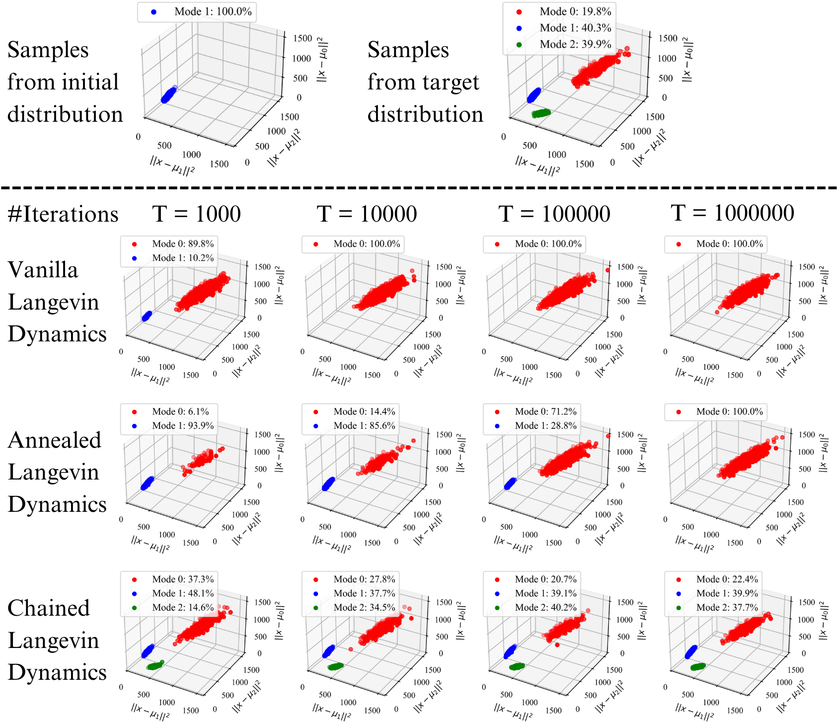
Figure 4: Samples from a mixture of three Gaussian modes generated by vanilla, annealed, and chained Langevin dynamics. Three axes are $\ell_{2}$ distance from samples to the mean of the three modes. The samples are initialized in mode 1.

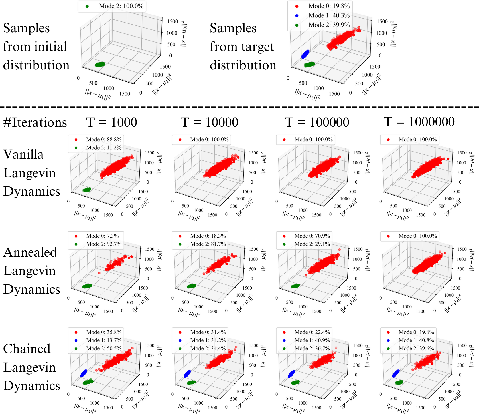
Figure 5: Samples from a mixture of three Gaussian modes generated by vanilla, annealed, and chained Langevin dynamics. Three axes are $\ell_{2}$ distance from samples to the mean of the three modes. The samples are initialized in mode 2.

Figure 6: Samples from a mixture distribution of the original and flipped images from the MNIST dataset generated by vanilla, annealed, and chained Langevin dynamics. The samples are initialized as flipped images from MNIST.

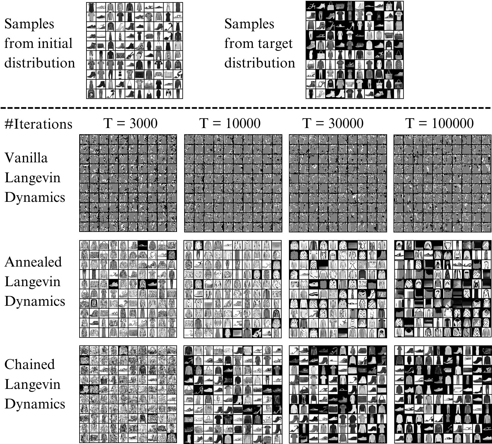
Figure 7: Samples from a mixture distribution of the original and flipped images from the Fashion-MNIST dataset generated by vanilla, annealed, and chained Langevin dynamics. The samples are initialized as flipped images from Fashion-MNIST.

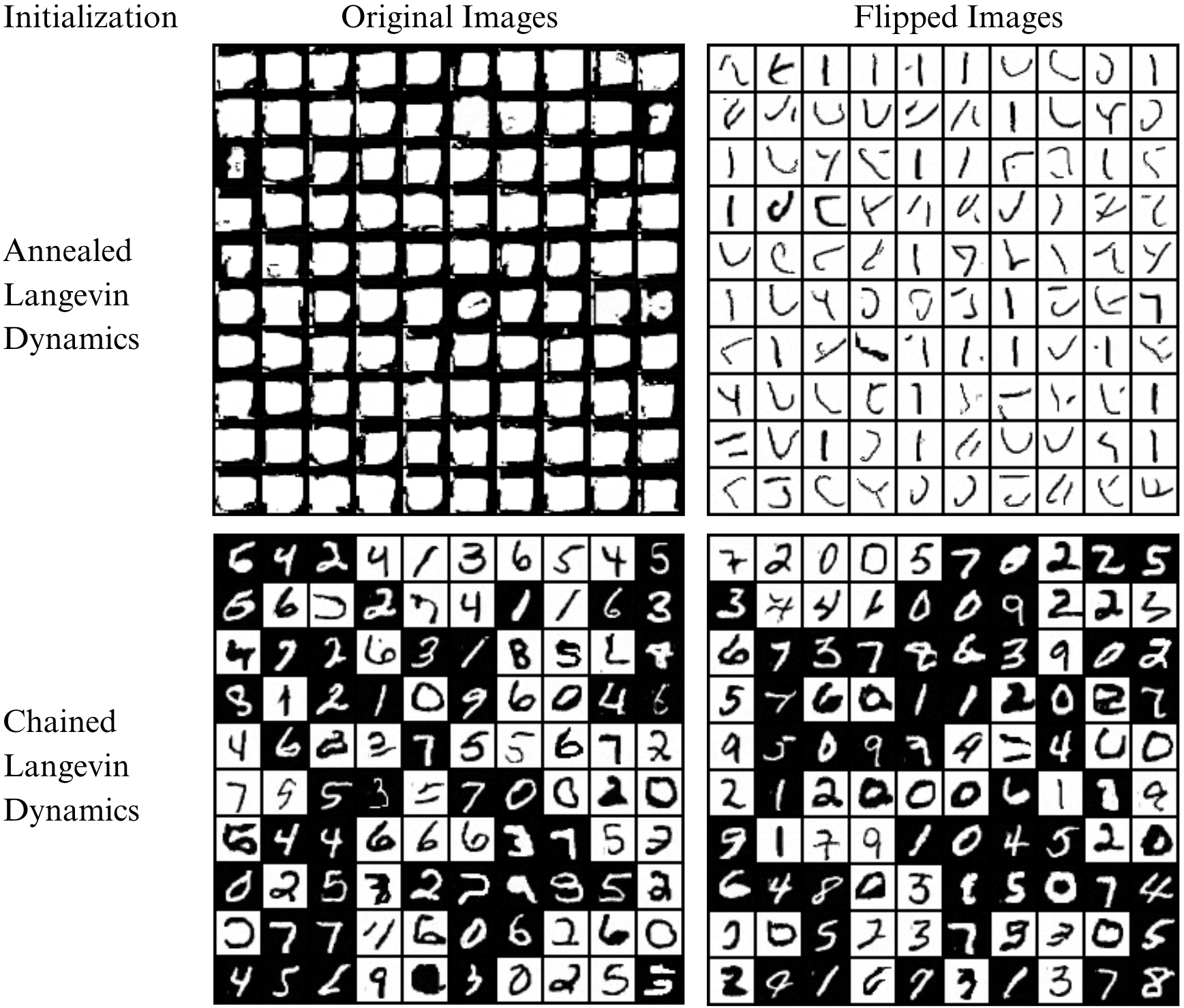
Figure 8: Samples from a mixture distribution of the original and flipped images from the MNIST dataset generated by annealed and chained Langevin dynamics for $T=100000$ iterations. The samples are initialized as the original or flipped images from MNIST.

Figure 9: Samples from a mixture distribution of the original and flipped images from the Fashion-MNIST dataset generated by annealed and chained Langevin dynamics for $T=100000$ iterations. The samples are initialized as the original or flipped images from Fashion-MNIST.

References

- [1] Yang Song, Jascha Sohl-Dickstein, Diederik P Kingma, Abhishek Kumar, Stefano Ermon, and Ben Poole. Score-based generative modeling through stochastic differential equations. In International Conference on Learning Representations, 2020.
- [2] Yang Song and Stefano Ermon. Generative modeling by estimating gradients of the data distribution. Advances in neural information processing systems, 32, 2019.
- [3] Yang Song and Stefano Ermon. Improved techniques for training score-based generative models. Advances in neural information processing systems, 33:12438–12448, 2020.
- [4] Jonathan Ho, Ajay Jain, and Pieter Abbeel. Denoising diffusion probabilistic models. Advances in neural information processing systems, 33:6840–6851, 2020.
- [5] Jiaming Song, Chenlin Meng, and Stefano Ermon. Denoising diffusion implicit models. arXiv preprint arXiv:2010.02502, 2020.
- [6] Aditya Ramesh, Prafulla Dhariwal, Alex Nichol, Casey Chu, and Mark Chen. Hierarchical text-conditional image generation with clip latents. arXiv preprint arXiv:2204.06125, 1(2):3, 2022.
- [7] Robin Rombach, Andreas Blattmann, Dominik Lorenz, Patrick Esser, and Björn Ommer. High-resolution image synthesis with latent diffusion models. In Proceedings of the IEEE/CVF conference on computer vision and pattern recognition, pages 10684–10695, 2022.
- [8] Nanxin Chen, Yu Zhang, Heiga Zen, Ron J Weiss, Mohammad Norouzi, and William Chan. Wavegrad: Estimating gradients for waveform generation. In International Conference on Learning Representations, 2020.
- [9] Zhifeng Kong, Wei Ping, Jiaji Huang, Kexin Zhao, and Bryan Catanzaro. Diffwave: A versatile diffusion model for audio synthesis. In International Conference on Learning Representations, 2020.
- [10] Jonathan Ho, William Chan, Chitwan Saharia, Jay Whang, Ruiqi Gao, Alexey Gritsenko, Diederik P Kingma, Ben Poole, Mohammad Norouzi, David J Fleet, et al. Imagen video: High definition video generation with diffusion models. arXiv preprint arXiv:2210.02303, 2022.
- [11] Andreas Blattmann, Robin Rombach, Huan Ling, Tim Dockhorn, Seung Wook Kim, Sanja Fidler, and Karsten Kreis. Align your latents: High-resolution video synthesis with latent diffusion models. In Proceedings of the IEEE/CVF Conference on Computer Vision and Pattern Recognition, pages 22563–22575, 2023.
- [12] Holden Lee, Jianfeng Lu, and Yixin Tan. Convergence for score-based generative modeling with polynomial complexity. Advances in Neural Information Processing Systems, 35:22870–22882, 2022.
- [13] Holden Lee, Jianfeng Lu, and Yixin Tan. Convergence of score-based generative modeling for general data distributions. In International Conference on Algorithmic Learning Theory, pages 946–985. PMLR, 2023.
- [14] Sitan Chen, Sinho Chewi, Jerry Li, Yuanzhi Li, Adil Salim, and Anru R Zhang. Sampling is as easy as learning the score: theory for diffusion models with minimal data assumptions. In International Conference on Learning Representations, 2023.
- [15] Gen Li, Yuting Wei, Yuxin Chen, and Yuejie Chi. Towards non-asymptotic convergence for diffusion-based generative models. In The Twelfth International Conference on Learning Representations, 2023.
- [16] Gen Li, Yu Huang, Timofey Efimov, Yuting Wei, Yuejie Chi, and Yuxin Chen. Accelerating convergence of score-based diffusion models, provably. arXiv preprint arXiv:2403.03852, 2024.
- [17] Max Welling and Yee W Teh. Bayesian learning via stochastic gradient langevin dynamics. In Proceedings of the 28th international conference on machine learning (ICML-11), pages 681–688. Citeseer, 2011.
- [18] Dawn B Wooddard, Scott C Schmidler, and Mark Huber. Conditions for rapid mixing of parallel and simulated tempering on multimodal distributions. The Annals of Applied Probability, 19(2):617–640, 2009.
- [19] Maxim Raginsky, Alexander Rakhlin, and Matus Telgarsky. Non-convex learning via stochastic gradient langevin dynamics: a nonasymptotic analysis. In Conference on Learning Theory, pages 1674–1703. PMLR, 2017.
- [20] Holden Lee, Andrej Risteski, and Rong Ge. Beyond log-concavity: Provable guarantees for sampling multi-modal distributions using simulated tempering langevin monte carlo. Advances in neural information processing systems, 31, 2018.
- [21] Christopher M Bishop. Pattern recognition and machine learning. Springer google schola, 2:645–678, 2006.
- [22] Liyiming Ke, Sanjiban Choudhury, Matt Barnes, Wen Sun, Gilwoo Lee, and Siddhartha Srinivasa. Imitation learning as f-divergence minimization. In Algorithmic Foundations of Robotics XIV: Proceedings of the Fourteenth Workshop on the Algorithmic Foundations of Robotics 14, pages 313–329. Springer, 2021.
- [23] Cheuk Ting Li and Farzan Farnia. Mode-seeking divergences: theory and applications to gans. In International Conference on Artificial Intelligence and Statistics, pages 8321–8350. PMLR, 2023.
- [24] Cheuk Ting Li, Jingwei Zhang, and Farzan Farnia. On convergence in wasserstein distance and f-divergence minimization problems. In International Conference on Artificial Intelligence and Statistics, pages 2062–2070. PMLR, 2024.
- [25] Anton Bovier, Michael Eckhoff, Véronique Gayrard, and Markus Klein. Metastability and low lying spectra in reversible markov chains. Communications in mathematical physics, 228:219–255, 2002.
- [26] Anton Bovier, Michael Eckhoff, Véronique Gayrard, and Markus Klein. Metastability in reversible diffusion processes i: Sharp asymptotics for capacities and exit times. Journal of the European Mathematical Society, 6(4):399–424, 2004.
- [27] Véronique Gayrard, Anton Bovier, and Markus Klein. Metastability in reversible diffusion processes ii: Precise asymptotics for small eigenvalues. Journal of the European Mathematical Society, 7(1):69–99, 2005.
- [28] RN Bhattacharya. Criteria for recurrence and existence of invariant measures for multidimensional diffusions. The Annals of Probability, pages 541–553, 1978.
- [29] Gareth O Roberts and Richard L Tweedie. Exponential convergence of langevin distributions and their discrete approximations. Bernoulli, pages 341–363, 1996.
- [30] D Bakry and M Émery. Diffusions hypercontractives. Seminaire de Probabilites XIX, page 177, 1983.
- [31] Dominique Bakry, Franck Barthe, Patrick Cattiaux, and Arnaud Guillin. A simple proof of the poincaré inequality for a large class of probability measures. Electronic Communications in Probability [electronic only], 13:60–66, 2008.
- [32] Arnak S Dalalyan. Theoretical guarantees for approximate sampling from smooth and log-concave densities. Journal of the Royal Statistical Society Series B: Statistical Methodology, 79(3):651–676, 2017.
- [33] Alain Durmus and Éric Moulines. Nonasymptotic convergence analysis for the unadjusted langevin algorithm. The Annals of Applied Probability, 27(3):1551–1587, 2017.
- [34] Santosh Vempala and Andre Wibisono. Rapid convergence of the unadjusted langevin algorithm: Isoperimetry suffices. Advances in neural information processing systems, 32, 2019.
- [35] Xiang Cheng, Niladri S Chatterji, Yasin Abbasi-Yadkori, Peter L Bartlett, and Michael I Jordan. Sharp convergence rates for langevin dynamics in the nonconvex setting. arXiv preprint arXiv:1805.01648, 2018.
- [36] Ian Goodfellow, Jean Pouget-Abadie, Mehdi Mirza, Bing Xu, David Warde-Farley, Sherjil Ozair, Aaron Courville, and Yoshua Bengio. Generative adversarial nets. Advances in neural information processing systems, 27, 2014.
- [37] Ian Goodfellow. Nips 2016 tutorial: Generative adversarial networks. arXiv preprint arXiv:1701.00160, 2016.
- [38] Ben Poole, Alexander A Alemi, Jascha Sohl-Dickstein, and Anelia Angelova. Improved generator objectives for gans. arXiv preprint arXiv:1612.02780, 2016.
- [39] Matt Shannon, Ben Poole, Soroosh Mariooryad, Tom Bagby, Eric Battenberg, David Kao, Daisy Stanton, and RJ Skerry-Ryan. Non-saturating gan training as divergence minimization. arXiv preprint arXiv:2010.08029, 2020.
- [40] Yang Song, Sahaj Garg, Jiaxin Shi, and Stefano Ermon. Sliced score matching: A scalable approach to density and score estimation. In Uncertainty in Artificial Intelligence, pages 574–584. PMLR, 2020.
- [41] Adam Block, Youssef Mroueh, and Alexander Rakhlin. Generative modeling with denoising auto-encoders and langevin sampling. arXiv preprint arXiv:2002.00107, 2020.
- [42] Valentin De Bortoli, James Thornton, Jeremy Heng, and Arnaud Doucet. Diffusion schrödinger bridge with applications to score-based generative modeling. Advances in Neural Information Processing Systems, 34:17695–17709, 2021.
- [43] Joe Benton, Valentin De Bortoli, Arnaud Doucet, and George Deligiannidis. Linear convergence bounds for diffusion models via stochastic localization. arXiv preprint arXiv:2308.03686, 2023.
- [44] Pascal Vincent. A connection between score matching and denoising autoencoders. Neural computation, 23(7):1661–1674, 2011.
- [45] Yann LeCun. The mnist database of handwritten digits. http://yann. lecun. com/exdb/mnist/, 1998.
- [46] Han Xiao, Kashif Rasul, and Roland Vollgraf. Fashion-mnist: a novel image dataset for benchmarking machine learning algorithms. arXiv preprint arXiv:1708.07747, 2017.
- [47] Olaf Ronneberger, Philipp Fischer, and Thomas Brox. U-net: Convolutional networks for biomedical image segmentation. In Medical image computing and computer-assisted intervention–MICCAI 2015: 18th international conference, Munich, Germany, October 5-9, 2015, proceedings, part III 18, pages 234–241. Springer, 2015.
- [48] Beatrice Laurent and Pascal Massart. Adaptive estimation of a quadratic functional by model selection. Annals of statistics, pages 1302–1338, 2000.
- [49] Guosheng Lin, Anton Milan, Chunhua Shen, and Ian Reid. Refinenet: Multi-path refinement networks for high-resolution semantic segmentation. In Proceedings of the IEEE conference on computer vision and pattern recognition, pages 1925–1934, 2017.
- [50] Haşim Sak, Andrew Senior, and Françoise Beaufays. Long short-term memory based recurrent neural network architectures for large vocabulary speech recognition. arXiv preprint arXiv:1402.1128, 2014.