Backward bifurcation arising from decline of immunity against emerging infectious diseases

Abstract

Decline of immunity is a phenomenon characterized by immunocompromised host and plays a crucial role in the epidemiology of emerging infectious diseases (EIDs) such as COVID-19. In this paper, we propose an age-structured model with vaccination and reinfection of immune individuals. We prove that the disease-free equilibrium of the model undergoes backward and forward transcritical bifurcations at the critical value of the basic reproduction number for different values of parameters. We illustrate the results by numerical computations, and also find that the endemic equilibrium exhibits a saddle-node bifurcation on the extended branch of the forward transcritical bifurcation. These results allow us to understand the interplay between the decline of immunity and EIDs, and are able to provide strategies for mitigating the impact of EIDs on global health.
Key words: backward bifurcation; decline of immunity; emerging infectious diseases

1 Introduction

The emergence of emerging infectious diseases (EIDs), such as COVID-19, has brought unprecedented challenges to the global health [1, 2]. To effectively control these diseases, we need to thoroughly understand the immune response against the pathogens involved. In ongoing research, a phenomenon known as backward bifurcation has attracted more and more attention, particularly in the context of decline of immunity associated with EIDs [3]. In mathematical epidemiology, a backward bifurcation occurs when the basic reproduction number is less than unity, in which case a small positive unstable endemic equilibrium appears while the disease-free equilibrium and a larger positive endemic equilibrium are locally asymptotically stable [4, 5, 6, 7]. The decline of immunity against EIDs refers to the waning of immunological responses over time, which can arise from the natural process of infection or the immune escape strategy adopted by the virus [1, 2]. Such decline may lead to the reinfection of immune individuals, especially in immunocompromised individuals [8]. The backward bifurcation provides a theoretical perspective for studying these dynamics, elucidating how the changes in parameters on immunity lead to bifurcations in the equilibrium states of disease transmission.

In this paper, we establish an age-structured model, which takes into account the reinfection of immune individuals due to the decline of immunity, and has the form

$$\left\{\begin{split}\frac{{\rm d}S}{{\rm d}t}\ &=\ \Lambda-\beta_{s}S\frac{\theta E+\epsilon A+I}{N}-(\alpha+u)S,\\ \frac{{\rm d}E}{{\rm d}t}\ &=\ \left(\beta_{s}S+\int^{\infty}_{0}\beta_{r}(\tau)r(t,\tau){\rm d}\tau\right)\frac{\theta E+\epsilon A+I}{N}-(\sigma+u)E,\\ \frac{{\rm d}A}{{\rm d}t}\ &=\ (1-\rho)\sigma E-(\gamma_{A}+u)A,\\ \frac{{\rm d}I}{{\rm d}t}\ &=\ \rho\sigma E-(\gamma_{I}+\mu+u)I,\\ \frac{\partial r}{\partial t}+\frac{\partial r}{\partial\tau}\ &=\ -\beta_{r}(\tau)\frac{\theta E+\epsilon A+I}{N}r-ur,\end{split}\right.$$ (1)

with the boundary condition

$$r(t,0)\ =\ \alpha S+\gamma_{A}A+\gamma_{I}I,$$ (2)

where the real-valued functions $S=S(t)$, $E=E(t)$, $A=A(t)$, and $I=I(t)$ denote the number of susceptible, latent, asymptomatic infected, and symptomatic infected individuals at time $t\geq 0$, respectively, and $r=r(t,\tau)$ denotes the density of immune individuals with immune age $\tau\geq 0$ at time $t$. The total population at time $t$ is denoted by $N(t):=S(t)+E(t)+A(t)+I(t)+\int^{\infty}_{0}r(t,\tau)\mbox{d}\tau$. We denote by $\Lambda>0$ the recruitment rate of susceptible individuals; $\mu,u>0$ are the death rate of symptomatic individuals and the natural death rate, respectively; $\sigma>0$ is the rate at which latent individuals progress to the next stage; $\gamma_{A},\gamma_{I}>0$ are the recovery rates of asymptomatic and symptomatic individuals, respectively; $\rho>0$ quantifies the proportion of symptomatic infected individuals; $\alpha>0$ is the vaccination rate of susceptible individuals; $\theta,\epsilon\in(0,1]$ are the coefficients for reduced transmission probabilities of latent and asymptomatic infected individuals, respectively; $\beta_{s}>0$ is the transmission rate of latent and infected individuals infecting susceptible individuals. Due to the gradual decline of immunity [9], the immune individuals are prone to be reinfected by the latent and infected individuals with the rate $\beta_{r}(\tau)(\theta E+\epsilon A+I)/N$ at the stage $\tau$. Hence, the dynamics of immune individuals can be described by the hyperbolic PDE (i.e., the last equation) in (1), where $\beta_{r}(\tau)>0$ is the transmission rate, and it is monotonically increasing and bounded, and thus $\beta_{r}\in L^{\infty}(0,\infty)$.

It is easy to prove that the solutions of (1) are non-negative with non-negative initial data. With the boundary condition (2), the disease-free equilibrium, denoted by $P_{0}$, is given by

$$P_{0}:=\left(S^{0},E^{0},A^{0},I^{0},r^{0}(\tau)\right)=\left(\frac{\Lambda}{\alpha+u},\ 0,\ 0,\ 0,\ \frac{\alpha\Lambda}{\alpha+u}{\rm e}^{-u\tau}\right).$$

The basic reproduction number (cf. [10, 11] for the details of computations) $\mathcal{R}_{0}$ is given by

$$\mathcal{R}_{0}=\frac{1}{(\sigma+u)N^{0}}\left(\beta_{s}S^{0}+\int^{\infty}_{0}\beta_{r}(\tau)r^{0}(\tau){\rm d}\tau\right)\left(\theta+\frac{(1-\rho)\sigma\epsilon}{\gamma_{A}+u}+\frac{\rho\sigma}{\gamma_{I}+\mu+u}\right),$$

where $N^{0}:=S^{0}+\int^{\infty}_{0}r^{0}(\tau){\rm d}\tau$. The rescaling $\beta_{r}(\tau)=\bar{\beta}\beta_{r0}(\tau)$ allows us to select the bifurcation parameter $\bar{\beta}>0$ with $\beta_{r0}(\tau)\in(0,1]$, and we set $\bar{\beta}^{*}$ is the value of $\bar{\beta}$ such that $\mathcal{R}_{0}=1$.

In this paper, we study the bifurcations of (1). Using Lyapunov-Schmidt reduction (cf., e.g., [12, 5]), we analytically prove the backward and forward transcritical bifurcations from $P_{0}$ at $\mathcal{R}_{0}=1$ for different values of parameters. In preparation for the main result of this paper, we define the following quantity which characterizes the quadratic nonlinearity of (1),

$$a:=\ \frac{2u}{\Lambda}\left(\theta+\frac{(1-\rho)\sigma\epsilon}{\gamma_{A}+u}+\frac{\rho\sigma}{\gamma_{I}+\mu+u}\right)\Bigg{[}\bar{\beta}^{*}\left(\frac{\alpha(\sigma+u)}{\alpha+u}+\frac{\gamma_{A}(1-\rho)\sigma}{\gamma_{A}+u}+\frac{\gamma_{I}\rho\sigma}{\gamma_{I}+\mu+u}\right)\int^{\infty}_{0}\beta_{r0}(\tau){\rm e}^{-u\tau}{\rm d}\tau$$

$$\quad-\frac{u}{\alpha+u}\left(\beta_{s}+\alpha\bar{\beta}^{*}\int^{\infty}_{0}\beta_{r0}(\tau){\rm e}^{-u\tau}{\rm d}\tau\right)\left(1+\frac{(1-\rho)\sigma}{u}+\frac{(\gamma_{I}+u)\rho\sigma}{\gamma_{I}+\mu+u}\right)$$ (3)

$$\quad-\frac{\alpha u}{\alpha+u}(\bar{\beta}^{*})^{2}\left(\theta+\frac{(1-\rho)\sigma\epsilon}{\gamma_{A}+u}+\frac{\rho\sigma}{\gamma_{I}+\mu+u}\right)\int^{\infty}_{0}\beta_{r0}(\tau){\rm e}^{-u\tau}\int^{\tau}_{0}\beta_{r0}(h)\,{\rm d}h\,{\rm d}\tau\Bigg{]},$$

and our main theorem is as follows.

Theorem 1.1

At $\mathcal{R}_{0}=1$, model (1) exhibits a backward transcritical bifurcation for $a>0$, and a forward transcritical bifurcation for $a<0$.

We remark that the quantity $a$ defined as in (1) is continuous in the parameters, thus $a$ can be zero. In such case, the transcritical bifurcation may degenerate into pitchfork bifurcations. However, this is beyond the scope of this paper and we do not pursue this further.

We illustrate the results in Theorem 1.1 with some numerical computations, which also suggest that the forward bifurcating branch extends to the point $\mathcal{R}_{0}=\mathcal{R}_{0}^{\rm bsn}>1$, at which the endemic equilibrium undergoes a saddle-node bifurcation; moreover, the bistable state, i.e., the coexistence of two stable endemic equilibria, occurs for some values of parameters.

This paper is organized as follows. In section 2, we give a proof of Theorem 1.1. We present some numerical computations in section 3 and provide a short discussion in section 4.

2 Bifurcation analysis

We consider the stationary solutions to (1) with the boundary condition (2). The proof is essentially based upon Lyapunov-Schmidt reduction, we refer the readers to, e.g., [12, 5], for more details.

We define the function space $X:=\mathbb{R}^{4}\times L^{1}(0,\infty)$, and the nonlinear operator $\mathcal{F}:X\times(0,\infty)\rightarrow X$ as follows

$$\mathcal{F}(\phi,\bar{\beta})=\begin{pmatrix}\Lambda-\beta_{s}S(\theta E+\epsilon A+I)/N-(\alpha+u)S\\ (\beta_{s}S+\bar{\beta}\int^{\infty}_{0}\beta_{r0}(\tau)r(t,\tau){\rm d}\tau)(\theta E+\epsilon A+I)/N-(\sigma+u)E\\ (1-\rho)\sigma E-(\gamma_{A}+u)A\\ \rho\sigma E-(\gamma_{I}+\mu+u)I\\ -\partial_{\tau}r-\bar{\beta}\beta_{r0}(\tau)r(\theta E+\epsilon A+I)/N-ur\end{pmatrix}$$

with $\phi=(S,E,A,I,r)^{\mathrm{T}}\in X$ and $\bar{\beta}\in(0,\infty)$. Linearizing $\mathcal{F}(\phi,\bar{\beta})$ in the disease-free equilibrium $\phi=P_{0}$ and evaluating at the parameter value $\bar{\beta}=\bar{\beta}^{*}$ gives the linear operator $\mathcal{A}:=\mathcal{F}_{\phi}(P_{0},\bar{\beta}^{*}):\mathcal{D}(\mathcal{A})\subset X\rightarrow X$ with the domain

$$\mathcal{D}(\mathcal{A}):=\mathbb{R}^{4}\times W^{1,1}(0,\infty),$$

which has the form

$$\mathcal{A}=\begin{pmatrix}-(\alpha+u)&-\theta D&-\epsilon D&-D&0\\ 0&\theta B-(\sigma+u)&\epsilon B&B&0\\ 0&(1-\rho)\sigma&-(\gamma_{A}+u)&0&0\\ 0&\rho\sigma&0&-(\gamma_{I}+\mu+u)&0\\ 0&-\theta\mathcal{E}(\tau)&-\epsilon\mathcal{E}(\tau)&-\mathcal{E}(\tau)&-(\partial_{\tau}+u)\end{pmatrix},$$

where $B:=(\beta_{s}S^{0}+\bar{\beta}^{*}\int^{\infty}_{0}\beta_{r0}(\tau)r^{0}(\tau){\rm d}\tau)/N^{0}$, $D:=\beta_{s}S^{0}/N^{0}$, $\mathcal{E}(\tau):=\bar{\beta}^{*}\beta_{r0}(\tau)r^{0}(\tau)/N^{0}$. It is easy to verify that $\mathcal{A}$ has a simple zero eigenvalue at $\mathcal{R}_{0}=1$ by considering the characteristic equation derived from the eigenvalue problem $\mathcal{A}x=\lambda x$ for non-trivial $x=(x_{1},x_{2},x_{3},x_{4},x_{5})^{\mathrm{T}}\in\mathcal{D}(\mathcal{A})$, subject to the boundary condition

$$x_{5}(0)=\alpha x_{1}+\gamma_{A}x_{3}+\gamma_{I}x_{4},$$ (4)

which stems from the linearization of (2) in $P_{0}$. Solving the equations $\mathcal{A}x=0$ with (4) gives the basis, denoted by $\hat{x}=(\hat{x}_{1},\hat{x}_{2},\hat{x}_{3},\hat{x}_{4},\hat{x}_{5})^{\mathrm{T}}\in\mathcal{D}(\mathcal{A})$, of the kernel of $\mathcal{A}$, i.e., $\ker(\mathcal{A})={\rm span}\{\hat{x}\}$, whose elements take the form

$$\hat{x}_{1} =-\frac{\beta_{s}S^{0}}{(\alpha+u)N^{0}}\left(\theta+\frac{(1-\rho)\sigma\epsilon}{\gamma_{A}+u}+\frac{\rho\sigma}{\gamma_{I}+\mu+u}\right),\quad\hat{x}_{2}=1,\quad\hat{x}_{3}=\frac{(1-\rho)\sigma}{\gamma_{A}+u},\quad\hat{x}_{4}=\frac{\rho\sigma}{\gamma_{I}+\mu+u},$$

$$\hat{x}_{5} =\hat{x}_{5}(\tau)=\left(\hat{x}_{5}(0)-\frac{\bar{\beta}^{*}}{N^{0}}\left(\theta+\frac{(1-\rho)\sigma\epsilon}{\gamma_{A}+u}+\frac{\rho\sigma}{\gamma_{I}+\mu+u}\right)\int^{\tau}_{0}\beta_{r0}(h)r^{0}(h){\rm e}^{uh}{\rm d}h\right){\rm e}^{-u\tau},$$

where the boundary value $\hat{x}_{5}(0)=\alpha\hat{x}_{1}+\gamma_{A}\hat{x}_{3}+\gamma_{I}\hat{x}_{4}$.

Next, we discuss the adjoint operator of $\mathcal{A}$, denoted by $\mathcal{A}^{*}$. Based upon the Riesz representation theorem on the identification of the dual space of $L^{1}$, we choose the function space $X^{*}:=\mathbb{R}^{4}\times L^{\infty}(0,\infty)$ and the domain of $\mathcal{A}^{*}$ as follows

$$\mathcal{D}(\mathcal{A}^{*}):=\mathbb{R}^{4}\times W^{1,\infty}(0,\infty)\subset X^{*}.$$

It is well-known that for all $x\in\mathcal{D}(\mathcal{A})$ and $\xi\in\mathcal{D}(\mathcal{A}^{*})$, the adjoint operator $\mathcal{A}^{*}$ is unique and satisfies $\langle\mathcal{A}x,\xi\rangle=\langle x,\mathcal{A}^{*}\xi\rangle$, where the bilinear form $\langle h,g\rangle:=\sum_{j=1}^{4}h_{j}g_{j}+\int_{0}^{\infty}h_{5}g_{5}\,{\rm d}\tau$ for any $h=(h_{1},\dots,h_{5})\in X$ and $g=(g_{1},\dots,g_{5})\in X^{*}$. Hence, for all $\xi=(\xi_{1},\xi_{2},\xi_{3},\xi_{4},\xi_{5})^{\mathrm{T}}\in\mathcal{D}(\mathcal{A}^{*})$ we have

$$\langle\mathcal{A}x,\xi\rangle\ =\ -\left[D(\theta x_{2}+\epsilon x_{3}+x_{4})+(\alpha+u)x_{1}\right]\xi_{1}+\left[B(\theta x_{2}+\epsilon x_{3}+x_{4})-(\sigma+u)x_{2}\right]\xi_{2}$$

$$\ +\left[(1-\rho)\sigma x_{2}-(\gamma_{A}+u)x_{3}\right]\xi_{3}+\left[\rho\sigma x_{2}-(\gamma_{I}+\mu+u)x_{4}\right]\xi_{4}$$

$$\ -\int^{\infty}_{0}\left[\mathcal{E}(\tau)(\theta x_{2}+\epsilon x_{3}+x_{4})+(\partial_{\tau}+u)x_{5}(\tau)\right]\xi_{5}(\tau)\,{\rm d}\tau$$

$$=\ -(\alpha+u)\xi_{1}x_{1}+\left[-\theta D\xi_{1}+\theta B\xi_{2}-(\sigma+u)\xi_{2}+(1-\rho)\sigma\xi_{3}+\rho\sigma\xi_{4}-\theta\mathcal{C}(\xi_{5})\right]x_{2}$$

$$\ +\left[-\epsilon D\xi_{1}+\epsilon B\xi_{2}-(\gamma_{A}+u)\xi_{3}-\epsilon\mathcal{C}(\xi_{5})\right]x_{3}+\left[-D\xi_{1}+B\xi_{2}-(\gamma_{I}+\mu+u)\xi_{4}-\mathcal{C}(\xi_{5})\right]x_{4}$$

$$\ -x_{5}(\infty)\xi_{5}(\infty)+x_{5}(0)\xi_{5}(0)+\int^{\infty}_{0}\big{[}\partial_{\tau}\xi_{5}(\tau)-u\xi_{5}(\tau)\big{]}x_{5}(\tau)\,{\rm d}\tau$$

$$=\ \langle x,\mathcal{A}^{*}\xi\rangle,$$

where the linear functional $\mathcal{C}(\xi_{5}):=\int_{0}^{\infty}\mathcal{E}(\tau)\xi_{5}(\tau)\,{\rm d}\tau$. Combining the condition (4) and the fact that $\lim_{\tau\to\infty}x_{5}(\tau)=0$ for $x_{5}\in W^{1,1}(0,\infty)$, the adjoint operator $\mathcal{A}^{*}:\mathcal{D}(\mathcal{A}^{*})\subset X^{*}\rightarrow X^{*}$ takes the form

$$\mathcal{A}^{*}=\begin{pmatrix}-(\alpha+u)&0&0&0&0\\ -\theta D&\theta B-(\sigma+u)&(1-\rho)\sigma&\rho\sigma&-\theta\mathcal{C}(\cdot)\\ -\epsilon D&\epsilon B&-(\gamma_{A}+u)&0&-\epsilon\mathcal{C}(\cdot)\\ -D&B&0&-(\gamma_{I}+\mu+u)&-\mathcal{C}(\cdot)\\ 0&0&0&0&\partial_{\tau}-u\end{pmatrix}$$

subject to the adjoint boundary conditions

$$\xi_{5}(0)=\xi_{5}(\infty)=0.$$

Solving the equations $\mathcal{A}^{*}\xi=0$ with such boundary conditions gives the eigenfunction in the kernel of $\mathcal{A}^{*}$, denoted by $\hat{\xi}$, which has the form

$$\hat{\xi}=\left(0,\ 1,\ \frac{\epsilon B}{\gamma_{A}+u},\ \frac{B}{\gamma_{I}+\mu+u},\ 0\right)^{\mathrm{T}}.$$

Differentiating $\mathcal{F}$ twice with respect to $\phi$ and evaluating at $\phi=P_{0}$, yields the bilinear form

$$\mathcal{F}_{\phi\phi}(P_{0},\bar{\beta})[x,y]=\left(\mathcal{H}_{1}[x,y],\ \mathcal{H}_{2}[x,y],\ 0,\ 0,\ \mathcal{H}_{3}[x,y]\right)^{\mathrm{T}},$$

where $y=(y_{1},y_{2},y_{3},y_{4},y_{5})^{\mathrm{T}}$ and

$$\mathcal{H}_{1}[x,y]\ =\ \frac{\beta_{s}(\theta x_{2}+\epsilon x_{3}+x_{4})[S^{0}(y_{1}+y_{2}+y_{3}+y_{4}+\int^{\infty}_{0}y_{5}(\tau){\rm d}\tau)-N^{0}y_{1}]}{(N^{0})^{2}}$$

$$\ +\frac{\beta_{s}(\theta y_{2}+\epsilon y_{3}+y_{4})[S^{0}(x_{1}+x_{2}+x_{3}+x_{4}+\int^{\infty}_{0}x_{5}(\tau){\rm d}\tau)-N^{0}x_{1}]}{(N^{0})^{2}},$$

$$\mathcal{H}_{2}[x,y]\ =\ -\frac{\bar{\beta}(\theta x_{2}+\epsilon x_{3}+x_{4})\int^{\infty}_{0}\beta_{r0}(\tau)[r^{0}(\tau)(y_{1}+y_{2}+y_{3}+y_{4}+\int^{\infty}_{0}y_{5}(h){\rm d}h)-N^{0}y_{5}(\tau)]{\rm d}\tau}{(N^{0})^{2}}$$

$$\ -\frac{\bar{\beta}(\theta y_{2}+\epsilon y_{3}+y_{4})\int^{\infty}_{0}\beta_{r0}(\tau)[r^{0}(\tau)(x_{1}+x_{2}+x_{3}+x_{4}+\int^{\infty}_{0}x_{5}(h){\rm d}h)-N^{0}x_{5}(\tau)]{\rm d}\tau}{(N^{0})^{2}}$$

$$\ -\mathcal{H}_{1}[x,y],$$

$$\mathcal{H}_{3}[x,y]\ =\ \frac{\bar{\beta}\beta_{r0}(\tau)(\theta x_{2}+\epsilon x_{3}+x_{4})[r^{0}(\tau)(y_{1}+y_{2}+y_{3}+y_{4}+\int^{\infty}_{0}y_{5}(\tau){\rm d}\tau)-N^{0}y_{5}]}{(N^{0})^{2}}$$

$$\ +\frac{\bar{\beta}\beta_{r0}(\tau)(\theta y_{2}+\epsilon y_{3}+y_{4})[r^{0}(\tau)(x_{1}+x_{2}+x_{3}+x_{4}+\int^{\infty}_{0}x_{5}(\tau){\rm d}\tau)-N^{0}x_{5}]}{(N^{0})^{2}}.$$

Differentiating $\mathcal{F}$ with respect to $\phi$ and $\bar{\beta}$, and evaluating at $\phi=P_{0}$, yields

$$\mathcal{F}_{\phi\bar{\beta}}(P_{0},\bar{\beta})x=\left(0,\ \frac{\int^{\infty}_{0}\beta_{r0}(\tau)r^{0}(\tau){\rm d}\tau(\theta x_{2}+\epsilon x_{3}+x_{4})}{N^{0}},\ 0,\ 0,\ -\frac{\beta_{r0}(\tau)r^{0}(\tau)(\theta x_{2}+\epsilon x_{3}+x_{4})}{N^{0}}\right)^{\mathrm{T}}.$$

Finally, we obtain the following quantities

$$\langle\mathcal{F}_{\phi\phi}(P_{0},\bar{\beta}^{*})[\hat{x},\hat{x}],\hat{\xi}\rangle\ =\ a,$$

$$\langle\mathcal{F}_{\phi\bar{\beta}}(P_{0},\bar{\beta}^{*})\hat{x},\hat{\xi}\rangle\ =\ \frac{1}{N^{0}}\left(\theta+\frac{(1-\rho)\sigma\epsilon}{\gamma_{A}+u}+\frac{\rho\sigma}{\gamma_{I}+\mu+u}\right)\int^{\infty}_{0}\beta_{r0}(\tau)r^{0}(\tau){\rm d}\tau>0.$$

where the expression of $a$ is given in (1). Hence, the bifurcation at $(\phi,\bar{\beta})=(P_{0},\bar{\beta}^{*})$ is transcritical, and the sign of $a$ determines the criticality of the bifurcation, cf., e.g., [12, 5].

3 Numerical bifurcation analysis

In order to illustrate and corroborate the analytical results, we present some numerical computations. We choose the values of parameters as follows [1, 2, 13]: $\Lambda=20000$, $\theta=0.55$, $\epsilon=0.55$, $u=1/(75\times 365)$, $\alpha=10^{-6}$, $\sigma=1/5.2$, $\rho=0.4$, $\gamma_{A}=1/14$, $\gamma_{I}=1/7$, $\mu=0.02$, and

$$\beta_{r0}(\tau)=\left\{\begin{split}&1-\eta,&&\tau<\hat{\tau},\\ &1-\eta{\rm e}^{-\gamma(\tau-\hat{\tau})},&&\tau\geq\hat{\tau},\end{split}\right.$$

where $\hat{\tau}=200$, $\eta=0.2$, and $\gamma=0.5$. To investigate the impact of $\mathcal{R}_{0}$ on the dynamics of (1), we plot the bifurcation diagram with the horizontal axis $\mathcal{R}_{0}$ by varying the bifurcation parameter $\bar{\beta}$ (due to the continuous dependence of $\mathcal{R}_{0}$ on $\bar{\beta}$), see Figure 1.

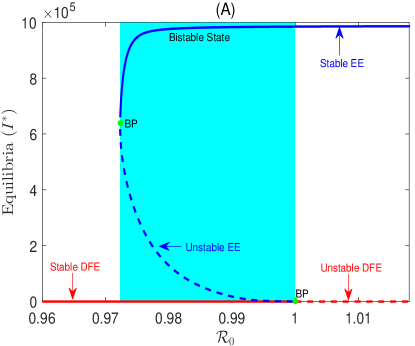
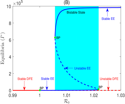
Figure 1: The number of symptomatic infected individuals at equilibria $I(t)=I^{*}$ varying with $\mathcal{R}_{0}$. (A) $\beta_{s}=0.1$ (i.e., $a=9.7232\times 10^{-6}>0$): the DFE undergoes the backward bifurcation at $\mathcal{R}_{0}=1$. (B) $\beta_{s}=0.10345$ (i.e., $a=-1.1558\times 10^{-5}<0$): the DFE undergoes the forward bifurcation at $\mathcal{R}_{0}=1$, and the saddle-node bifurcation arises from the stable EE at $\mathcal{R}_{0}=\mathcal{R}_{0}^{\rm bsn}\approx 1.0218$. Green dots: bifurcation point; cyan regions: the bistable state exists.

We first consider the case $\beta_{s}=0.1$ (i.e., $a=9.7232\times 10^{-6}>0$), the bifurcation from the disease-free equilibrium (DFE) at $\mathcal{R}_{0}=1$ is backward transcritical, and the bifurcating branch extends backward to $\mathcal{R}_{0}=\mathcal{R}_{0}^{\rm fsn}\approx 0.9723$, at which a saddle-node bifurcation occurs; moreover, for $\mathcal{R}_{0}\in(\mathcal{R}_{0}^{\rm fsn},1)$ model (1) exhibits the bistable state, in which case a stable endemic equilibrium (EE) and a stable DFE coexist, cf., Figure 1(A). This indicates, for $\mathcal{R}_{0}\in(\mathcal{R}_{0}^{\rm fsn},1)$, that the transmission of the infectious disease can be controlled only with sufficiently small initial number of symptomatic infected individuals (SIIs).

Next, we consider the case $\beta_{s}=0.10345$ (i.e., $a=-1.1558\times 10^{-5}<0$), the bifurcation from the DFE at $\mathcal{R}_{0}=1$ is forward transcritical, moreover, the bifurcating branch extends forward to $\mathcal{R}_{0}=\mathcal{R}_{0}^{\rm bsn}\approx 1.0218$, at which the saddle-node bifurcation occurs and its bifurcating branch extends backward to the other saddle-node bifurcation point at $\mathcal{R}_{0}=\mathcal{R}_{0}^{\rm fsn}\approx 1.0057$, cf., Figure 1(B). The numerical computations also suggest, that (i) for $\mathcal{R}_{0}\in(1,\mathcal{R}_{0}^{\rm fsn})$ the number of SIIs remains small; (ii) for $\mathcal{R}_{0}\in(\mathcal{R}_{0}^{\rm fsn},\mathcal{R}_{0}^{\rm bsn})$ model (1) exhibits the bistable state, in which case two stable EEs coexist, and thus the number of SIIs converges to the lower and upper stable EEs for sufficiently small and large initial data, respectively; (iii) for $\mathcal{R}_{0}>\mathcal{R}_{0}^{\rm bsn}$ the number of SIIs always converges to the upper stable EE. These results indicate that $\mathcal{R}_{0}=\mathcal{R}_{0}^{\rm fsn}$ is the first critical threshold beyond which the disease can be severe for sufficiently large initial number of SIIs, and $\mathcal{R}_{0}=\mathcal{R}_{0}^{\rm bsn}$ is the second critical threshold beyond which the disease becomes severe regardless of the initial number of SIIs.

4 Conclusion

In this paper, we have developed the immune age-structured model (1) that takes into account the decline of immunity. Using Lyapunov-Schmidt reduction, we have proved the backward and forward transcritical bifurcations for different values of parameters. We have also presented some numerical computations on various bifurcations, which allow us to explore the nonlinear relations between the immune parameters and the equilibrium of disease. In particular, we found that the saddle-node bifurcation occurs on the extended branch of the forward transcritical bifurcation, and two stable endemic equilibria coexist for some values of parameters.

These results can help us to obtain a deeper understanding of the dynamics of emerging infectious diseases. Incorporating such immunological factors, we are able to gain insights into the conditions that favor disease persistence and severity. We found that the initial number of infected individuals plays a crucial role in determining the disease severity, which emphasizes the importance of early detection and containment. Targeting high-risk individuals and implementing timely interventions may mitigate the impact of emerging infectious diseases and contain their spread.

References

[1]
L. Xue, S. Jing, K. Zhang, R. Milne, H. Wang, Infectivity versus fatality of
SARS-CoV-2 mutations and influenza, International Journal of Infectious
Diseases 121 (2022) 195–202.
[2]
S. Jing, R. Milne, H. Wang, L. Xue, Vaccine hesitancy promotes emergence of new
SARS-CoV-2 variants, Journal of Theoretical Biology 570 (2023) 111522.
[3]
I. M. Wangari, Emergence of a reversed backward bifurcation, reversed
hysteresis effect, and backward bifurcation phenomenon in a COVID-19
mathematical model, Mathematical Methods in the Applied Sciences 47 (4)
(2024) 2250–2272.
[4]
M. Martcheva, An Introduction to Mathematical Epidemiology, Vol. 61, Springer,
New York, 2015.
[5]
M. Martcheva, H. Inaba, A Lyapunov–Schmidt method for detecting backward
bifurcation in age-structured population models, Journal of Biological
Dynamics 14 (1) (2020) 543–565.
[6]
C. Castillo-Chavez, B. Song, Dynamical models of tuberculosis and their
applications, Mathematical Biosciences and Engineering 1 (2) (2004) 361–404.
[7]
J. Yang, M. Zhou, X. Li, Backward bifurcation of an age-structured epidemic
model with partial immunity: the Lyapunov–Schmidt approach, Applied
Mathematics Letters 133 (2022) 108292.
[8]
S. Rahman, M. M. Rahman, M. Miah, M. N. Begum, M. Sarmin, M. Mahfuz, M. E.
Hossain, M. Z. Rahman, M. J. Chisti, T. Ahmed, et al., COVID-19
reinfections among naturally infected and vaccinated individuals, Scientific
Reports 12 (1) (2022) 1438.
[9]
M. Risk, S. S. Hayek, E. Schiopu, L. Yuan, C. Shen, X. Shi, G. Freed, L. Zhao,
COVID-19 vaccine effectiveness against omicron (B.1.1.529) variant
infection and hospitalisation in patients taking immunosuppressive
medications: a retrospective cohort study, The Lancet Rheumatology 4 (11)
(2022) e775–e784.
[10]
P. van den Driessche, J. Watmough, Reproduction numbers and sub-threshold
endemic equilibria for compartmental models of disease transmission,
Mathematical Biosciences 180 (1-2) (2002) 29–48.
[11]
O. Diekmann, J. A. P. Heesterbeek, J. A. Metz, On the definition and the
computation of the basic reproduction ratio in models for
infectious diseases in heterogeneous populations, Journal of Mathematical
Biology 28 (4) (1990) 365–382.
[12]
H. Kielhöfer, Bifurcation Theory: An Introduction with Applications to
Partial Differential Equations, Springer, New York, 2012.
[13]
Y. Wu, W. Zhou, S. Tang, R. A. Cheke, X. Wang, Prediction of the next major
outbreak of COVID-19 in Mainland China and a vaccination strategy for
it, Royal Society Open Science 10 (8) (2023) 230655.