Neural Green’s Operators for Parametric Partial Differential Equations

Abstract

This work introduces neural Green’s operators (NGOs), a novel neural operator network architecture that learns the solution operator for a parametric family of linear partial differential equations (PDEs). Our construction of NGOs is derived directly from the Green’s formulation of such a solution operator. Similar to deep operator networks (DeepONets) and variationally mimetic operator networks (VarMiONs), NGOs constitutes an expansion of the solution to the PDE in terms of basis functions, that is returned from a sub-network, contracted with coefficients, that are returned from another sub-network. However, in accordance with the Green’s formulation, NGOs accept weighted averages of the input functions, rather than sampled values thereof, as is the case in DeepONets and VarMiONs. Application of NGOs to canonical linear parametric PDEs shows that, while they remain competitive with DeepONets, VarMiONs and Fourier neural operators when testing on data that lie within the training distribution, they robustly generalize when testing on finer-scale data generated outside of the training distribution. Furthermore, we show that the explicit representation of the Green’s function that is returned by NGOs enables the construction of effective preconditioners for numerical solvers for PDEs.

1 Introduction

In this paper, we consider the problem of inferring the solution operator, associated with a parametric family of partial differential equations (PDEs), from data. Generally, the task of approximating such solution operators plays a fundamental role in the development of computational methods for solving the underlying PDEs [1, 2] that appear in various areas of science and engineering. Typical examples include computational fluid dynamics [3], fluid-structure interaction [4] and solid mechanics [5]. However, finding analytical expressions of such solution operators is generally not feasible, and numerical approximations of such operators can be computationally prohibitive due to their high-dimensional and nonlinear nature [1]. Recent advances in operator learning techniques [6] address this challenge by using data to approximate solution operators to PDEs. Typically, the data is comprised of instantiations of solutions to the PDE and the corresponding PDE input functions, such as boundary conditions, PDE coefficients and external forcings. The inference problem is to find the operator that maps the PDE parameters to the solution. If such a mapping is inferred, we are able to evaluate it and recover solutions of the PDE for different input parameters. However, to formulate the operator learning problem, we need a suitable representation of PDE solution mappings between function spaces.

By virtue of their generalization of standard neural networks [7] to mappings between function spaces instead of between discrete vector spaces, neural operators (NOs) [6] provide a suitable representation of PDE solution maps. Representation of operators by NOs can be roughly divided into categories: the first approach expands the output function in terms of the dot product between two vectors that are returned from two sub-networks, the so-called branch and trunk networks, which accept as arguments samples of the input functions and spatial coordinates, respectively; the second approach replaces the discrete affine transformation in a standard deep neural network by an integral operator with a non-local kernel, which allows the network to accept functions, rather than samples thereof, as input. The former construction is due to that work in [8] and was extended to deep-operator-networks (DeepONets) in [9], while the latter construction was developed for different choices of the nonlocal kernel functions such as the Fourier [10], multipole [11] and graph [12], neural operators (FNOs, MNOs and GNOs, respectively). Both such approaches received considerable research attention, and significant work has been devoted to their extensions and improvements [6]. Moreover, both approaches have been successfully applied to approximating solutions to PDEs, such as PDEs for fluid-mechanics [13], fluid-structure-interaction [14], solid-mechanics [15] and quantum-mechanics [16]. However, by construction, such NOs approximate the action of the solution operator on the input functions, but do not provide an explicit representation of the solution operator. Such an explicit representation of PDE solution operators may be used to construct closures for multiscale or coupled models, stabilize numerical methods [1] or to accelerate numerical solvers [17].

Here, we focus on linear PDEs where the corresponding solution operator reduces to the Green’s operator with the Green’s function as the corresponding kernel [18]. Significant research work has been devoted to inferring an explicit representation of Green’s functions for PDEs, e.g. in [19], an SVD-based manifold-interpolation approach is used to recover Green’s functions on data comprised of PDE solutions; in [20] and [21], Green’s functions of linear PDEs are represented by neural networks; in [22], autoencoders are used infer a matrix representation of the linearized PDE operator to a non-linear PDE, where the inverse of such a matrix represents the Green’s function. However, such approximations of Green’s functions do not account for the nonlinear dependence of the Green’s function on some of the input PDE parameters such as the PDE coefficients, i.e. these networks are trained for a particular instantiation of such parameters. On the other hand, variationally mimetic operator networks (VarMiONs [23]) yield a representation of the Green’s operator that is parameterized by the PDE coefficients. However, the number of trainable parameters in VarMiON scales unfavorably with the number of sampling points used for the input functions. Such a scaling is unfavorable for systems where a dense sampling of input functions is required which may result in inefficient models.

In this work, we introduce a paradigm for constructing NOs that are based on a finite-dimensional representation of Green’s operators with a learnable Green’s function, we refer to such NOs as neural Green’s operators (NGOs). Our construction of NGOs accepts weighted-averages of functions, rather than samples thereof, as input. We ask the question whether our construction of NGOs leads to improved generalization of our NO to unseen and out-of-distribution data, and whether we can utilize the inferred Green’s functions in a different context, such as accelerating (classical) numerical PDE solvers (e.g. iterative solvers for the method of finite elements, finite volumes, finite differences, spectral elements, …etc.). Thereafter we demonstrate that:

1. NGO-based networks enable efficient approximations of PDE solutions in the sense that for roughly the same number of network parameters, NGOs yield approximations that generalize in a significantly more robust manner than DeepONets, VarMiONs and FNOs.

2. The Green’s functions inferred from NGO-based networks can be used to construct effective matrix-preconditioners for numerical PDE solvers.

The remainder of this paper is organized as follows: section 2, introduces Green’s operators for parametric PDEs and corresponding finite-dimensional representations of the Green’s function. In section 3 we introduce the architecture of NGO-based networks in terms a learnable matrix. In section 4 we describe a test problem and the corresponding data generation and training procedure. In section 5, we provide results on the model accuracy, the effect of quadrature and computational efficiency. Additionally, we demonstrate the construction of matrix-preconditioners from the learned Green’s function, as well as their effectiveness. We end with a concluding discussion in section 6.

2 Parametric Green’s Operators and Functions

In this paper, we consider linear boundary value problem in a bounded domain $\Omega\subset\mathbb{R}^{d}$ with a piecewise smooth boundary $\Gamma=\bigcup_{i}\Gamma_{i}$:

$$\mathcal{L}[\theta]u(\mathbf{x}) =f(\mathbf{x}) \forall\mathbf{x}\in\Omega$$ (2.1)

$$\mathcal{B}_{i}[\theta]u(\mathbf{x}) =g_{i}(\mathbf{x}) \forall\mathbf{x}\in\Gamma_{i},$$

where $u(\mathbf{x})$ denotes the unknown, $\mathcal{L}[\theta]$ is a linear differential operator, parameterized by some spatially varying coefficient $\theta(\mathbf{x})$, $f(\mathbf{x})$ is a source term, $\mathcal{B}_{i}[\theta]$ is a boundary operator, and $g_{i}$ is the data on the boundary $\Gamma_{i}$.

To find an expression for the unknown $u(\mathbf{x})$, we write (2.1) in weak form by testing the first equation of (2.1) against some suitable function $v$:

$$\int_{\Omega}v\mathcal{L}[\theta]u\,d\mathbf{x}=\int_{\Omega}vf\,d\mathbf{x}.$$ (2.2)

Using integration by parts and substituting the boundary conditions we may arrive at the formulation

$$\int_{\Omega}u\mathcal{L}^{*}[\theta]v\,d\mathbf{x}-\sum_{i}\int_{\Gamma\setminus\Gamma_{i}}(\mathcal{B}_{i}[\theta]u)(\tilde{\mathcal{B}}_{i}v)\,d\mathbf{x}=\int_{\Omega}vf\,d\mathbf{x}+\sum_{i}\int_{\Gamma_{i}}g_{i}\tilde{\mathcal{B}}_{i}v\,d\mathbf{x}.$$ (2.3)

where $\mathcal{L}^{*}$ is the adjoint operator of $\mathcal{L}$, and $\tilde{\mathcal{B}}_{i}$ are boundary operators that appear in the integration by parts.

We can derive an expression for the unknown $u(\mathbf{x})$ by setting $v$ in (2.3) to be the Green’s function $G[\theta](\mathbf{x},\mathbf{x}^{\prime})$ that satisfies

$$\mathcal{L}^{*}[\theta]G[\theta](\mathbf{x},\mathbf{x}^{\prime}) =\delta(\mathbf{x}-\mathbf{x}^{\prime}) \forall\mathbf{x}\in\Omega$$ (2.4)

$$\tilde{\mathcal{B}}_{i}G[\theta](\mathbf{x},\mathbf{x}^{\prime}) =0 \forall\mathbf{x}\in\Gamma\setminus\Gamma_{i}.$$

Then, (2.3) reduces to

$$u(\mathbf{x}^{\prime})=\mathcal{G}[\theta,f,g_{i}](\mathbf{x}^{\prime}):=\int_{\Omega}G[\theta]f\,d\mathbf{x}+\sum_{i}\int_{\Gamma_{i}}g_{i}\tilde{\mathcal{B}}_{i}G[\theta]\,d\mathbf{x},$$ (2.5)

and $\mathcal{G}$ denotes the Green’s operator that maps the PDE coefficient $\theta(\mathbf{x})$, forcing $f(\mathbf{x})$ and boundary data $g_{i}$ onto the solution $u(\mathbf{x})$ [18].

To derive a finite-dimensional approximation of the solution, we consider an expansion of the Green’s function in terms of a test-basis $\phi_{m}(\mathbf{x})$ and trial-basis $\psi_{n}(\mathbf{x}^{\prime})$ as

$$G[\theta](\mathbf{x},\mathbf{x}^{\prime})\approx\psi_{n}(\mathbf{x}^{\prime})A_{mn}[\theta]\phi_{m}(\mathbf{x}),$$ (2.6)

where $A_{mn}$ depends nonlinearly on $\theta$. Substitution of (2.6) into (2.5) gives the corresponding approximation of the Green’s operator

$$\mathcal{G}[\theta,f,g_{i}](\mathbf{x}^{\prime})\approx A_{mn}[\theta]d_{m}[f,g_{i}]\psi_{n}(\mathbf{x}^{\prime}),$$ (2.7)

where

$$d_{m}[f,g_{i}]=\int_{\Omega}\phi_{m}fd\mathbf{x}+\sum_{i}\int_{\Gamma_{i}}g_{i}\tilde{\mathcal{B}}_{i}\phi_{m}\,d\mathbf{x}.$$ (2.8)

Remark 1.

In a Galerkin approximation setting, the matrix $A_{mn}$ in (2.6) represents the inverse of the system matrix.

Remark 2.

While our approximation of the Green’s function in (2.6) conforms to a Petrov-Galerkin method where the test functions $\phi$ and trial functions $\psi$ are not the same, we may opt for a (Bubnov-)Galerkin setting for our NGO, where $\phi$ and $\psi$ are the same.

3 Neural Green’s Operators

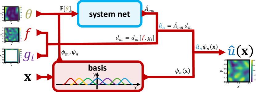
We now define a Neural Green’s operator, based on the approximation in (2.6) with a learnable matrix, and fixed test functions $\phi(\mathbf{x})$ and trial functions $\psi(\mathbf{x})$:

$$\hat{u}(\mathbf{x})=\hat{\mathcal{G}}[\theta,f,g_{i}](\mathbf{x})\equiv\hat{A}_{mn}(\mathbf{F}[\theta])d_{m}[f,g_{i}]\psi_{n}(\mathbf{x}),$$ (3.1)

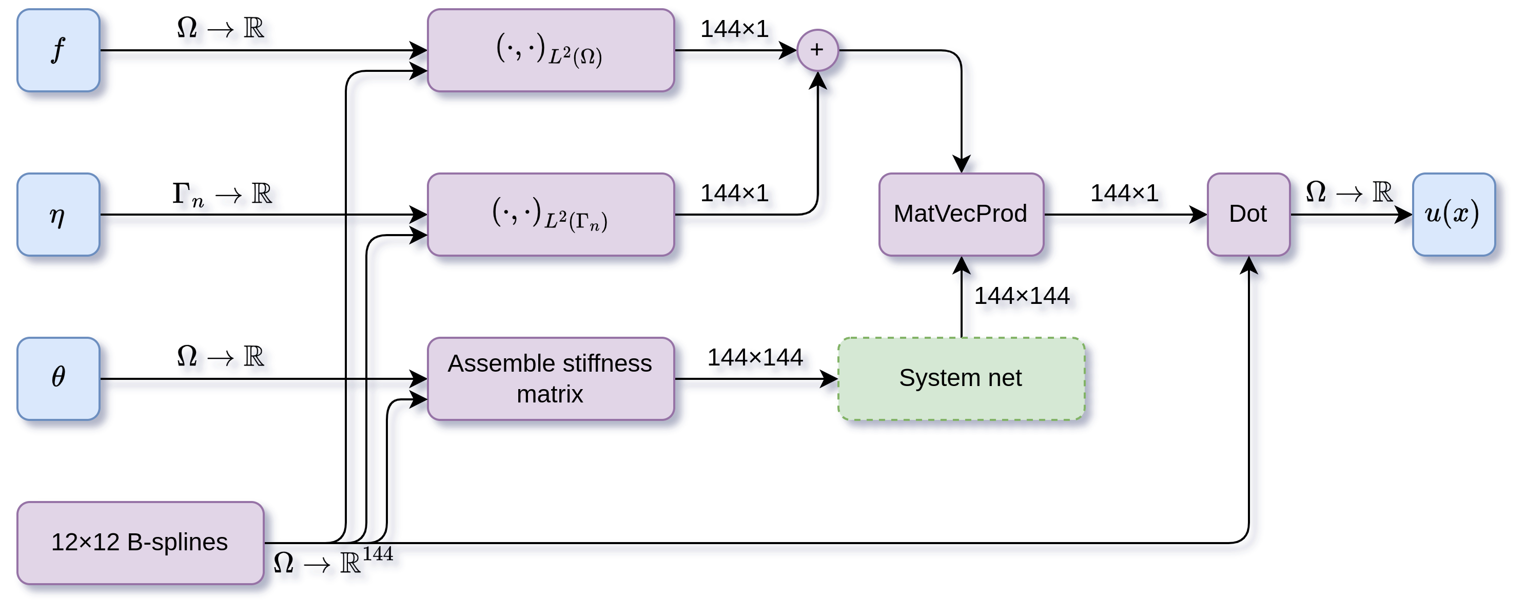
where ‘hats’ indicate quantities learned by a neural network. Based on the specific form of $\mathbf{F}[\theta]$, we distinguish between two types of NGOs. The first type is the model-NGO, where we set

$$\mathbf{F}[\theta]=\int_{\Omega}\psi_{n}\mathcal{L}^{*}[\theta]\phi_{m}\,d\mathbf{x}-\int_{\Gamma\setminus\Gamma_{i}}(\mathcal{B}_{i}[\theta]\psi_{n})(\tilde{\mathcal{B}}_{i}\phi_{m})\,d\mathbf{x},$$ (3.2)

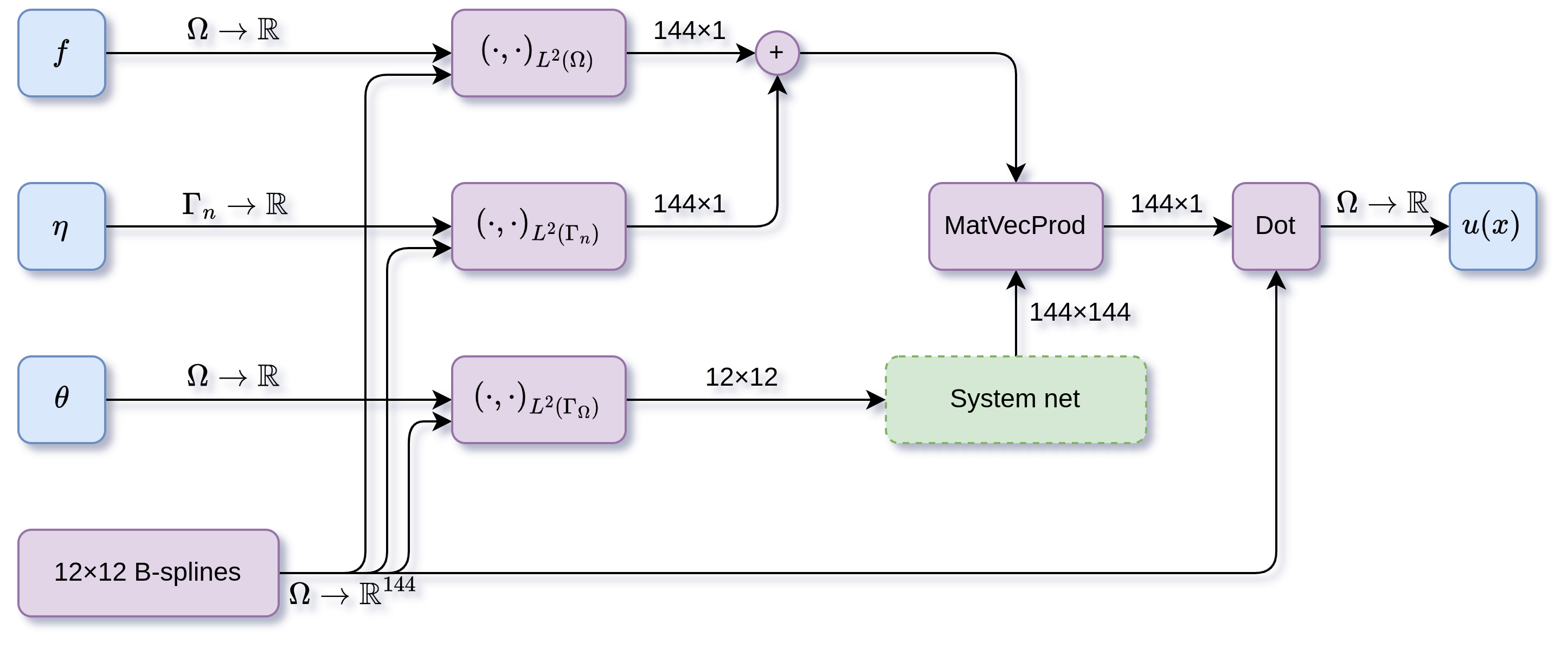
which represents the system-matrix corresponding to a discretization of (2.3). A model-NGO can be used when the PDE (2.1) that underlies the NGO training data is known. On the other hand, we consider a second type of NGO, referred to as a data-NGO, which may be used if the PDE that underlies the training data is not known, where

$$\mathbf{F}[\theta]=\int_{\Omega}\phi_{m}\theta d\mathbf{x}.$$ (3.3)

We summarize the NGO architecture in Figure 1.

Figure 1: Architecture of the neural Green’s operator (NGO), that maps the material parameter $\theta(\mathbf{x})$, forcing $f(\mathbf{x})$ and boundary conditions $g_{i}(\mathbf{x})$ onto the solution $u(\mathbf{x})$. For a model-NGO, $\mathbf{F}$ is given by (3.2), whereas for a data-NGO, $\mathbf{F}$ is given by (3.3). The system-network, shown in blue, is the only machine learning based component in the NGO.

Remark 3.

While our NGO in (3.1) uses fixed bases, we may opt to learn either the test function $\phi$ or the trial function $\psi$, or both.

4 Test Problem: Darcy Equation

In this section, we compare the performance of the NGO with other models in literature, including DeepONets, VarMiONs, and FNOs. The test equation is a Darcy flow equation on a unit square, with varying material properties $\theta$. The boundary conditions are inhomogeneous Neumann boundary conditions on the top and bottom boundaries, and homogeneous Dirichlet on the left and right boundaries.

$$-\nabla\cdot\left(\theta\nabla u\right) =f\text{ on }\Omega=(0,1)^{2}$$ (4.1a)

$$\theta\nabla u\cdot\mathbf{n} =\eta\text{ on }\Gamma_{n}=(0,1)\times\left\{0,1\right\}$$ (4.1b)

$$u =0\text{ on }\Gamma_{d}=\left\{0,1\right\}\times(0,1)$$ (4.1c)

All neural operators were trained to learn the solution operator $\left(\theta,f,\eta\right)\mapsto u$.

4.1 Data Generation

To test the efficacy of different model architectures, three different data sets were generated.

• For the first dataset, $N=10000$ random triples $\left(\theta,f,\eta\right)$ were sampled, and the resulting PDE was solved to obtain $u$. The functions $\theta$ were obtained by sampling $10000$ independent functions $\hat{\theta}$ from a Gaussian Random Field (GRF) with correlation length $\lambda=0.4$, after which $\theta$ was defined as $\theta_{i}(\mathbf{x})=a\hat{\theta}(\mathbf{x})+b$, where the scalars $a,b$ were chosen such that $\theta$ lies in the interval $[0.02,0.99]$, i.e. $\min_{i}\min_{\mathbf{x}}\theta_{i}(\mathbf{x})=0.02$ and $\max_{i}\max_{\mathbf{x}}\theta_{i}(\mathbf{x})=0.99$. The source terms $f$ were generated using the same process, except with $\lambda=0.2$. Finally $\eta$ was generated in the same way with $\lambda=0.3$ and the resulting functions were scaled and shifted to lie in $[-1,1]$.

  To solve the PDEs, we made use of the Nutils [24] finite element solver. The domain was discretised on a $20\times 20$ grid of cubic B-splines (resulting in $23^{2}$ basis functions). Comparing the solutions to those obtained on a $40\times 40$ grid, we found that the numerical solutions have a relative error of about $3\cdot 10^{-4}$.

• For the second dataset, solutions were obtained using manufactured solutions [25]. In this approach, the solution $u$ and the parameters $\theta$ are randomly generated, after which the source and boundary terms are computed by evaluating the relevant differential operator acting on $u$. Firstly, the functions $\theta$ were generated in using the same method as was used in the previous dataset, but with smaller characteristic length scale $\lambda=0.2$. Then, random functions $\hat{u}$ were generated from a GRF with $\lambda=0.2$, and the solutions were given as $u_{i}(\mathbf{x})=x_{1}\left(1-x_{1}\right)\hat{u}_{i}(\mathbf{x})$, to ensure that the solutions satisfy the homogeneous Dirichlet boundaries exactly. Then, $f$ and $\eta$ were simply computed by evaluating their corresponding operators in (4.1) through analytical expressions for the relevant derivatives. Finally, for each sample we scale $f_{i}$, $\eta_{i}$, and $u_{i}$ uniformly so that $\|f_{i}\|_{L^{2}}=\frac{1}{2}$. This normalisation was done to ensure that the inputs $\eta,\theta,f$ are of a similar magnitude to what they are in the training data. For the VarMiON and NGO, the normalisation doesn’t affect the model accuracy since these models are linear in $f$ and $\eta$. However, DeepONets and FNOs, which do not have this linearity, are expected to perform best when the inputs are of a similar magnitude to the training data.

The first data set will be used for training, validation, and testing, while the second data set will be used only for testing. The reason for this distinction is to test how well models trained on one data set can generalise to differently distributed data. When using models as preconditioners in numerical methods, the expectation is that the model will be used on problems that do not lie in the training data distribution. As such, generalisation to such data is considered an important factor for models used as preconditioners.

(a) Finite element data set

(b) Manufactured data set

Figure 2: Five random samples of solutions from both the finite element data set (left) and the manufactured data set (right).

4.2 Model Architectures

The solution to (4.1) can be expressed in terms of the Green’s function as

$$u(\mathbf{x})=\int_{\Omega}G[\theta](\mathbf{x},\mathbf{x}^{\prime})f(\mathbf{x}^{\prime})d\mathbf{x}^{\prime}+\int_{\Gamma_{n}}G[\theta](\mathbf{x},\mathbf{x}^{\prime})\eta(\mathbf{x}^{\prime})d\mathbf{x}^{\prime}-\int_{\Gamma_{d}}g\hat{\mathbf{n}}\cdot\nabla G[\theta]d\mathbf{x}^{\prime}.$$ (4.2)

Using the ansatz in (2.6) to approximate the Green’s function in (4.2), with $\phi_{m}=\psi_{m}$, we can approximate the solution

$$u(\mathbf{x})=\mathcal{G}[\theta,f,\eta,g](\mathbf{x})\approx A_{mn}[\theta]d_{m}[f,\eta,g]\psi_{n}(\mathbf{x}),$$ (4.3)

where $d_{m}$ is given by

$$d_{m}[f,\eta,g]=\int_{\Omega}\psi_{m}fd\mathbf{x}^{\prime}+\int_{\partial\Omega_{\eta}}\psi_{m}\eta d\mathbf{x}^{\prime}-\int_{\Gamma_{d}}g\hat{\mathbf{n}}\cdot\nabla\psi_{m}d\mathbf{x}^{\prime}.$$ (4.4)

We define the NGO corresponding to (4.3) as

$$\hat{u}(\mathbf{x})=\hat{\mathcal{G}}[\theta,f,\eta,g](\mathbf{x})=\hat{A}_{mn}[\theta]d_{m}[f,\eta,g]\psi_{n}(\mathbf{x}).$$ (4.5)

In the next section we compare the performance of the NGO in (4.5) to that of VarMiONs, DeepONets and FNOs. The exact architecture of these models are given in Appendix A.

4.3 Training Procedure

The training procedure was the same for each model. The model is trained on the first 8000 samples of the first dataset. After every epoch, the model was evaluated on the validation data (another 1000 samples from the first data). The final trained model was the model that performed the best on the validation data. Table 1 shows the training configuration.

Loss function	Relative $L^{2}$ error
Optimiser	ADAM
Learning rate	Default ($10^{-3}$)
Batch size	100
Training time	20000 epochs
Training data	Samples $1-8000$
Validation data	Samples $8001-9000$
Testing data (in distribution)	Samples $9001-10000$
Testing data (out of distribution)	All 1000 manufactured samples

Table 1: Configuration of the training procedure

5 Results

5.1 Model Accuracy

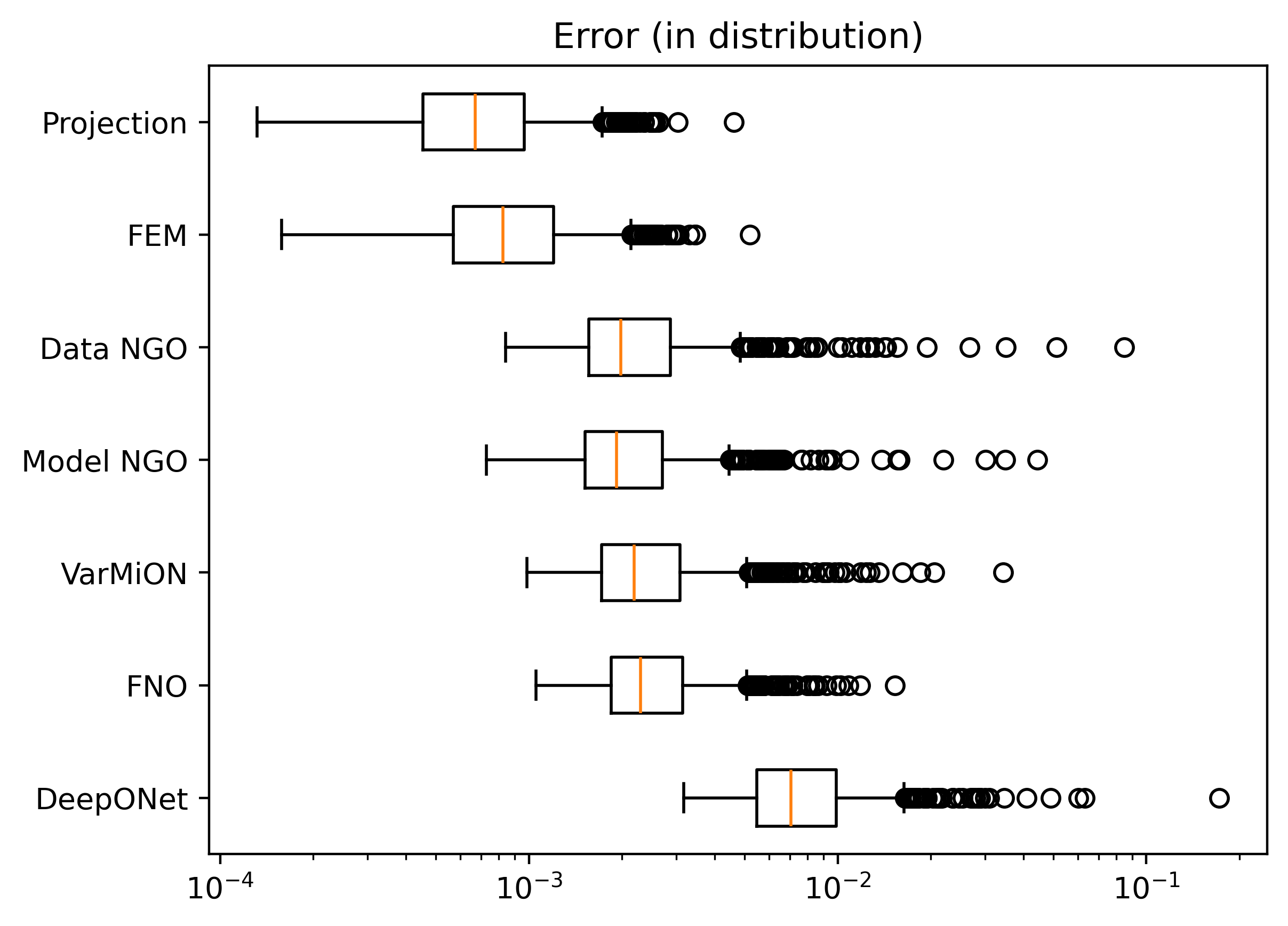
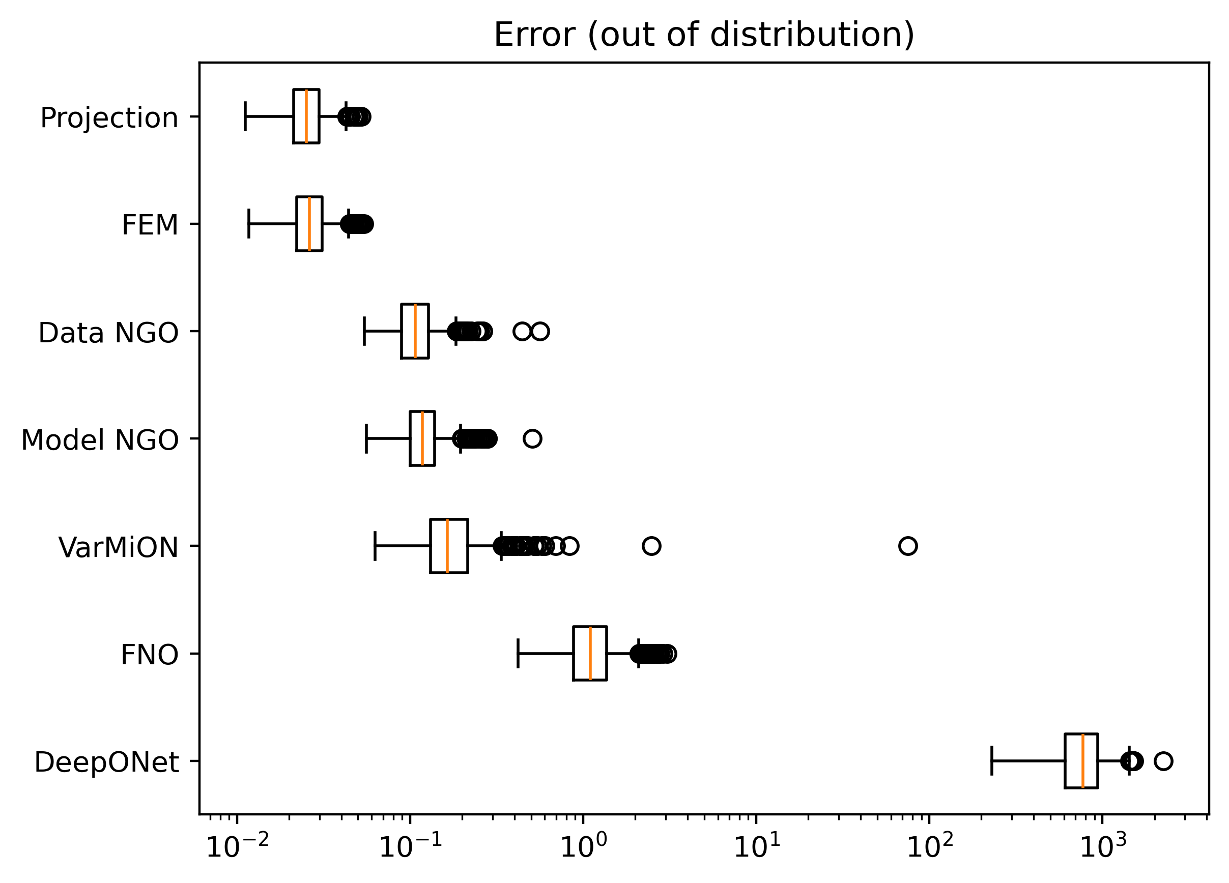
Table 2 shows the error percentages achieved by the trained models on the in-distribution and out-of-distribution testing data sets. The errors are given in terms of mean and standard deviation of the relative $L^{2}$ error. For some model and data set, if $u^{(i)},i=1,\dots,N$ are the true solutions and $\hat{u}^{(i)}$ are the model predictions, we define the relative $L^{2}$ error as $e_{i}=\frac{\|\hat{u}^{(i)}-u^{(i)}\|_{L^{2}(\Omega)}}{\|u^{(i)}\|_{L^{2}(\Omega)}}$. The distribution of errors is also shown in Figure 3.

As a reference, Table 2 and Figure 3 also include the accuracy obtained by the Finite Element Method (FEM) using the same $12\times 12$ cubic B-spline basis functions, as well as the error obtained by projecting the true solutions onto the span of the basis functions. The “Projection” entry is therefore the lowest possible error achievable by any model using these basis functions.

Model	Parameters	Test error
		In distribution	Out of distribution
DeepONet	31224	$0.86\%\pm 0.73\%$	$\phantom{}78751.55\%\pm\phantom{}25143.43\%$
FNO	31721	$0.27\%\pm 0.14\%$	$\phantom{00}117.12\%\pm\phantom{000}41.39\%$
VarMiON	31283	$0.27\%\pm 0.20\%$	$\phantom{000}25.91\%\pm\phantom{00}236.82\%$
Model NGO	28387	$0.24\%\pm 0.24\%$	$\phantom{000}12.29\%\pm\phantom{0000}3.49\%$
Data NGO	27981	$0.26\%\pm 0.37\%$	$\phantom{000}11.22\%\pm\phantom{0000}3.59\%$
FEM	–	$0.10\%\pm 0.06\%$	$\phantom{0000}2.70\%\pm\phantom{0000}0.67\%$
Projection	–	$0.08\%\pm 0.05\%$	$\phantom{0000}2.59\%\pm\phantom{0000}0.64\%$

Table 2: Overview of the accuracy of the tested models on different data sets. The ‘FEM’ entry shows the solution errors of solving the PDEs with finite elements on the B-spline basis used by the DeepONet, VarMiON, and NGOs. The ‘Projection’ entry shows the error when projecting the true solution onto the B-spline basis, which is therefore the lowest error achievable by any model using this basis.

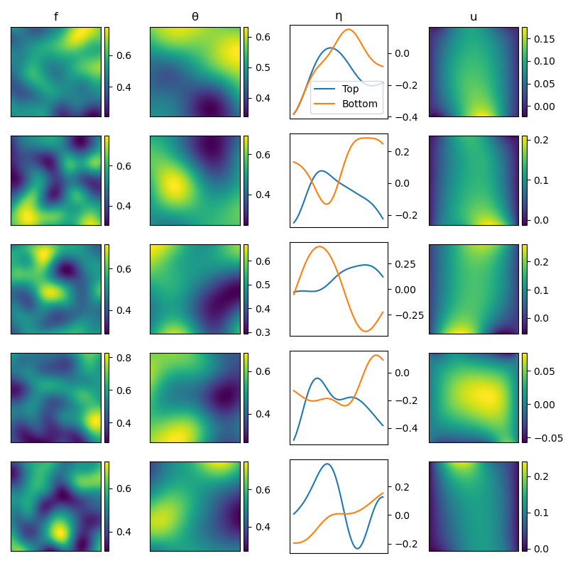
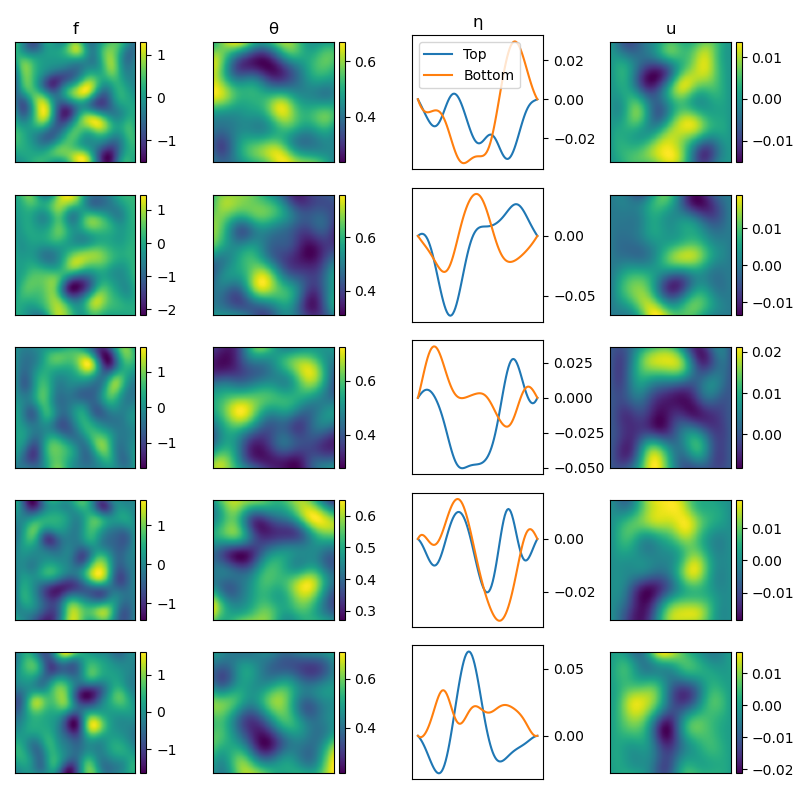
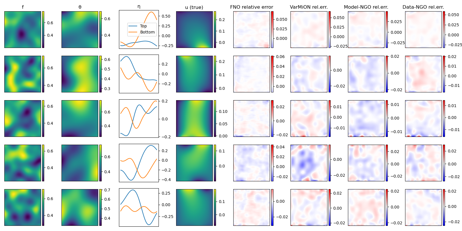
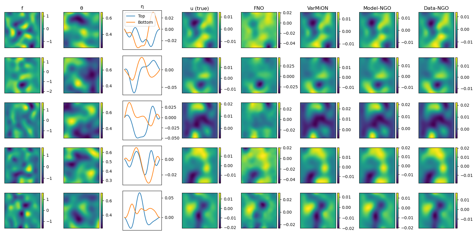
Figure 4 shows five random samples from the in-distribution testing data, along with the relative errors in the predictions of the FNO, VarMiON, and NGOs. The predicted solutions themselves are omitted in this figure, since they are all visually indistinguishable from each other and from the true solutions. Similarly, Figure 5 shows example problems, true solutions, and predicted solutions from the out-of-distribution testing data. In this figure, it is clear that the VarMiON and NGOs still produce predictions that are visually accurate, whereas the FNO’s predictions are noticeably different from the true solutions.

Figure 3: Error box plots of the different models on the heat equation problem.

Figure 4: True solution and relative solution error of four different models, tested on five random samples from the in-distribution testing data set. The model predictions themselves are omitted here as they are visually indistinguishable from each other and from the true solutions.

Figure 5: True solution and predicted solutions of four different models, tested on five random samples from the out-of-distribution data set.

5.2 Effect of Quadrature and Training Error

The accuracy of the NGO predictions is determined by different error sources, that collectively add up to the total prediction error. In this section, we analyse the effect of quadrature error and training error on the NGO accuracy. We use a dataset that consists of 10000 manufactured solutions with length scales that lie in the range $0.5\leq\lambda/L\leq 1$, in which both the Neumann and Dirichlet boundary conditions are varied.

In Figure 6, we compare the accuracy of DeepONets, VarMiONs and model NGOs on manufactured solution test datasets of the Darcy equation with varying GRF length scales $\lambda/L$, where $L$ is the box size of the domain $\Omega$.

Figure 6: Relative L2 error comparison between DeepONets, VarMiONs and model NGOs that use the same 8x8 cubic B-spline basis, and have roughly the same number of 3e4 trainable parameters, but use different uniform (U) or Gauss-Legendre (G-L) quadrature grids of different densities. Every data point represents the average score on a manufactured test dataset of 100 samples with scaled GRF length scale $\lambda/L$, where $L$ is the box size of the domain $\Omega$, and the error bars are 95% confidence intervals. For the smaller out of training data distribution length scales $\lambda/L\lessapprox 0.2$, only the NGOs with the dense 100x100 quadrature grids can stay close to the (lowerst achievable) L2 projection errors.

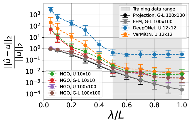
All models use a 8x8 cubic B-spline basis, and have roughly the same number of 3e4 trainable parameters, but use different uniform or Gauss-Legendre quadrature grids. The models are trained on dataset 3. The black data represents the $L^{2}$ projection of the ground truth solutions onto the B-spline basis, and therefore the lowest error achievable by neural operators that use this basis. Within and outside of the training data range, all NGOs outperform the DeepONet and VarMiON. More interestingly, for test data of length scales $\lambda/L\lessapprox 0.2$, we see that only the NGOs with the finest 100x100 quadrature grids are the closest to the lowest achievable projection errors. Whereas we observed a finite element simulation with a Gauss-Legendre 100x100 quadrature grid to be significantly more accurate than a finite element simulation with a 100x100 uniform quadrature grid, the quadrature rule turns out to be of minor importance for the accuracy of an NGO prediction.

An important feature of an NGO is that its model size in terms of trainable parameters is invariant to the quadrature density: the quadrature can be refined without changing the neural network architecture, and thereby, at zero cost of extra trainable parameters. Model sizes of other neural operator architectures like DeepONets and VarMiONs inevitably grow when the quadrature density is increased. For example, if we had increased the quadrature density of the DeepONet to 100x100, the number of trainable parameters would have grown with two orders of magnitude.

Let $Q=n$ denote a $n\times n$ grid, figures 7 and 8 show examples of predictions of model NGOs with sparse $Q=10$ and dense $Q=100$ Gauss-Legendre quadrature, of a smooth solution of $\lambda/L=0.5$, and a rough solution of $\lambda=0.1$, respectively. In Figure 7, the $L^{2}$ projection of the true solution shows that the $u$ is well-represented on the coarse 8x8 cubic B-spline basis, and both the $Q=10$ and $Q=100$ NGOs have accurate enough quadrature to accurately reproduce $u$.

Figure 7: From left to right: example of a test GRF sample $u$ with a length scale of $\lambda/L=0.5$, the L2 projection of $u$ onto the 8x8 cubic B-spline basis used by the NGOs, and the predicted solutions by model NGOs that use $Q=10$ (a 10x10 grid, corresponding to 2x2 per element) and $Q=100$ (a 100x100 grid, corresponding to 20x20 per element) Gauss-Legendre quadrature grids, respectively. On this smooth test sample, the quadrature of both NGOs is fine enough to correctly reproduce the true solution $u$.

In Figure 8, the projection shows that the rough solution is under-resolved by the coarse basis.

Figure 8: From left to right: example of a test GRF sample $u$ with a length scale of $\lambda/L=0.1$, the L2 projection of $u$ onto the 8x8 cubic B-spline basis used by the NGOs, and the predicted solutions by model NGOs that use $Q=10$ (a 10x10 grid, corresponding to 2x2 per element) and $Q=100$ (a 100x100 grid, corresponding to 20x20 per element) Gauss-Legendre quadrature grids, respectively. The $L^{2}$ projection provides the $L^{2}$ optimal representation of the true solution on the coarse basis, however, the mesh is clearly under-resolved. While the $Q=10$ NGO provides an inaccurate solution, the $Q=100$ NGO manages to provide a solution that is visually close to the L2 projection.

The $Q=10$ NGO provides an inaccurate prediction of the true solution, however, the $Q=100$ NGO manages to provide a solution that is visually close to the $L^{2}$ projection of the true solution. Therefore, with sufficient quadrature density, NGOs yield predictions that are closer to the $L^{2}$ projection of the true solution than VarMiONs and DeepONets.

In Figure 6, it is visible that the NGO errors do not follow the projection error trend for larger $\lambda/L$, but instead flatten out to a constant value. To demonstrate that this constant error value is dictated by training error, we compare the relative $L^{2}$ errors of different $Q=100$ Gauss-Legendre NGOs, that have been trained for different numbers of epochs, in Figure 9.

Figure 9: Relative L2 error comparison between $Q=100$ Gauss-Legendre model NGOs that have been trained for different numbers of epochs. Every data point represents the average score on a manufactured test dataset of 100 samples with scaled GRF length scale $\lambda/L$, where $L$ is the box size of the domain $\Omega$, and the error bars are 95% confidence intervals. Even for longer training times, the prediction errors for larger $\lambda/L$ stays finite. This is a result of training error (limited approximation capacity of the system net).

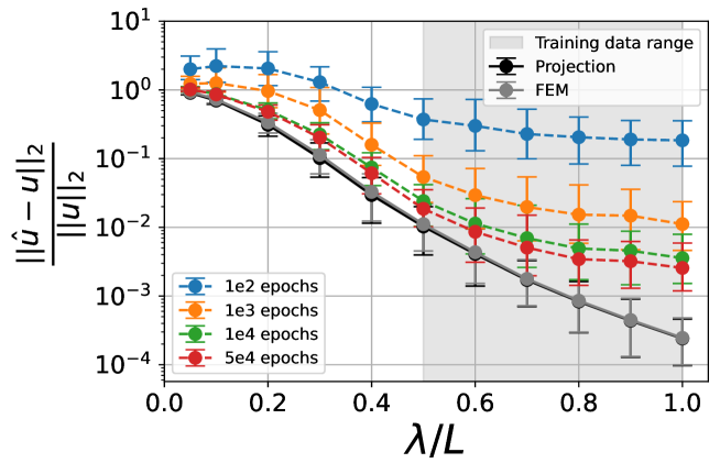
We see that the longer the model has been trained, the closer the NGO prediction errors get to the optimal $L^{2}$ projection errors. However, we also observe that the predication errors stagnate as the number of epochs grows, which suggests that we are observing the limited approximation capacity of the system network, for a well-trained model. An analysis of the training error as a function of the number of trainable parameters, and for different system net architectures, is left for future work.

5.3 Training Speed

In addition to the accuracy of different models, we also compare the model architectures by their computational efficiency. To do this, the VarMiON, FNO, and NGO variants are benchmarked on a server with a 28-core 2.6GHz Intel Xeon Gold 6132 CPU and four NVIDIA Tesla V100 GPUs. The training performance is measured by evaluating the model on a batch of 100 samples, and also performing the back-propagation necessary for gradient-based optimisation. Note that NGOs first compute inner products of the PDE parameters with the basis functions or their derivatives. This step comes at a measurable computational cost, but does not depend on any trainable parameters of the models. As such, it is possible to precompute these vectors and matrices for a given data set, and train the NGO by passing it these precomputed arrays directly during training. The NGO performance is tested with this optimisation implemented.

Table 3 shows the training and inference performance of FNOs, VarMiONs, as well as Model-NGOs and Data-NGOs. From this, it is clear that the VarMiON is the fastest model to train, followed by the NGOs. Furthermore, the VarMiON and NGOs have much lower memory usage than the FNO.

Model	Memory usage (GB)	Throughput (batches/sec)
FNO	4.14	9.1
VarMiON	0.24	121.0
Model-NGO	0.51	53.6
Data-NGO	0.33	101.9

Table 3: Memory usage and throughput of different models. For the NGOs, the assembly of the system network inputs was done ahead of time.

5.4 NGO-based Preconditioners

An advantage of NGOs is that due to the fact that they learn an approximation to the Green’s function, trained NGOs are not only useful as surrogate models but can also be used to construct preconditioners for numerical discretisations of the same PDE. In this section, we give an example of using a trained NGO to construct a preconditioner for a finite difference discretisation for the diffusion equation. Specifically, a given discretisation of a PDE yields a linear system with a matrix $\mathbf{A}(\theta)$, for which we can construct a right preconditioner $\mathbf{P}(\theta)$ from the NGO, such that the condition number of $\mathbf{AP}$ is much smaller than that of $\mathbf{A}$.

For this example, we take the same equation, this time with constant $\theta=\frac{1}{2}$ for simplicity. We will formulate a simple finite difference discretisation of this PDE, and use the Data-NGO trained in the previous section to construct a preconditioner. For the finite difference discretisation, we assume a uniform grid (i.e. $\Delta x=\Delta y\equiv h$) and use the five-point difference scheme to approximate the second derivative:

$$-\nabla\cdot(\theta\nabla u)=-\frac{1}{2}\Delta u \approx\frac{1}{2h^{2}}\left(u_{i,j+1}+u_{i,j-1}+u_{i+1,j}+u_{i-1,j}-4u_{i,j}\right).$$

We take $h=\frac{1}{49}$, which produces a discretisation with $50$ points along the $y$-direction and $48$ points along the $x$-direction (since the Dirichlet boundary conditions mean that the boundary points do not need to be included). This produces a linear system $\mathbf{A}\vec{x}=\vec{b}$, where

$$\mathbf{A} =\mathbf{A}_{x}\otimes\mathcal{I}_{50}+\mathcal{I}_{48}\otimes\mathbf{A}_{y}$$

$$\mathbf{A}_{x} =\frac{1}{h^{2}}\begin{bmatrix}-2&1&&&\\ 1&-2&1&&\\ &1&-2&\ddots&\\ &&\ddots&\ddots&1\\ &&&1&-2\end{bmatrix}, \mathbf{A}_{y} =\frac{1}{h^{2}}\begin{bmatrix}-2&2&&&\\ 1&-2&1&&\\ &1&-2&\ddots&\\ &&\ddots&\ddots&1\\ &&&2&-2\end{bmatrix},$$

$$\vec{x}_{50(i-1)+j} =u(x_{i},y_{j}), \vec{b}_{50(i-1)+j} =f(x_{i},y_{j})$$

$$x_{i} =ih, y_{j} =(j-1)h.$$

Here, for clarity of notation, we use the arrow notation for vectors, and we will use that throughout the remainder of this section as well. The linear system has $N=2400$ unknowns, which is much larger than the $n=144$ basis functions of the NGO. Importantly, this means that we cannot directly apply the NGO as a preconditioner: since the NGO learns an operator of rank at most $144$, applying it as a preconditioner directly would result in a singular system, which does not have a unique solution.

Nevertheless, we can use the trained NGO to construct a preconditioner $\mathbf{P}$ such that $\kappa(\mathbf{AP})\ll\kappa(\mathbf{A})$. Generally, discretised differential operators produce ill-conditioned matrices since they amplify high-frequency components while dampening low-frequency components. As such, a preconditioning strategy is to construct a preconditioner $\mathbf{P}$ that amplifies the low frequencies, while preserving the high-frequencies. To construct such a preconditioner, we first write the learned Green’s function in a singular value decomposition (SVD) form.

1. For the given parameters $\theta$, the NGO learns an approximation to the Green’s operator as

   $$G_{\theta}(x,y) \approx\sum_{i,j=1}^{n}\varphi_{i}(x)\mathbf{M}_{ij}(\theta)\varphi_{j}(y).$$

2. Now, we first orthonormalise the function basis: define the Gram matrix $\mathbf{G}_{ij}=\int_{\Omega}\varphi_{i}(x)\varphi_{j}(x)~{}dx$, and take the Cholesky decomposition $\mathbf{G}=\mathbf{LL}^{\top}$. Then define $\tilde{\varphi}_{i}(x)=\sum_{j}\mathbf{L}^{-1}_{ij}\varphi_{j}(x)$, which gives us a representation of the learned Green’s function in terms of an orthonormal basis:

   $$G_{\theta}(x,y) \approx\sum_{i,j=1}^{n}\tilde{\varphi}_{i}(x)\left(\mathbf{L}^{\top}\mathbf{M}(\theta)\mathbf{L}\right)_{ij}\tilde{\varphi}_{j}(y).$$

3. Next, we compute an SVD of the inner matrix: $\mathbf{L}^{\top}\mathbf{M}(\theta)\mathbf{L}=\mathbf{U}\bm{\Sigma}\mathbf{V}^{\top}$, with $\mathbf{U}$ and $\mathbf{V}$ orthogonal matrices and $\bm{\Sigma}=\text{diag}(\sigma_{1},\sigma_{2},\dots,\sigma_{n})$:

   $$G_{\theta}(x,y) \approx\sum_{i,j=1}^{n}\tilde{\varphi}_{i}(x)\left(\mathbf{U}\bm{\Sigma}\mathbf{V}^{\top}\right)_{ij}\tilde{\varphi}_{j}(y).$$

   We can then define two additional orthonormal bases, by merging the factors $\mathbf{U}$ and $\mathbf{V}$ into the basis $\tilde{\varphi}_{i}$:

   $$\tilde{\varphi}^{(U)}_{j} =\sum_{i}\tilde{\varphi}_{i}\mathbf{U}_{ij}$$

   $$\tilde{\varphi}^{(V)}_{j} =\sum_{i}\tilde{\varphi}_{i}\mathbf{V}_{ij}$$

   $$G_{\theta}(x,y) \approx\sum_{i=1}^{n}\tilde{\varphi}^{(U)}_{i}(x)\sigma_{i}\tilde{\varphi}^{(V)}_{i}(y).$$

Now, we focus on the orthonormal basis functions $\tilde{\varphi}^{(U)}_{i}$: these are the left singular functions corresponding to the largest singular values of $G$, and will therefore correspond to the lowest singular values of the differential operator $\mathbf{A}$. We now want a preconditioner that, when given a vector $\vec{u}$ corresponding to a function $u(x)$, amplifies the low-frequency components in $u$ that correspond to the basis functions $\tilde{\varphi}^{(U)}$, while preserving the higher frequency components. For a function $u$, its decomposition into low and high frequencies is as follows:

$$u(x) =\underbrace{\sum_{i}\left\langle\tilde{\varphi}^{(U)}_{i},u\right\rangle\tilde{\varphi}^{(U)}_{i}(x)}_{\text{low frequencies}}+\underbrace{\left[u(x)-\sum_{i}\left\langle\tilde{\varphi}^{(U)}_{i},u\right\rangle\tilde{\varphi}^{(U)}_{i}(x)\right]}_{\text{high frequencies}},$$

where the orthonormality of the basis $\tilde{\varphi}^{(U)}$ is crucial in making the separation easy to compute. To do this separation in the discrete setting, we sample the functions $\tilde{\varphi}^{(U)}_{i}$, producing a matrix $\bm{\Phi}\in\mathbb{R}^{N\times n}$, and replace the $L^{2}$ inner products in $\Omega$ by a quadrature rule with weights $\mathbf{W}\in\mathbb{R}^{N}$:

$$\vec{u} =\underbrace{\bm{\Phi}\bm{\Phi}^{\top}\text{diag}(W)\vec{u}}_{\text{low frequencies}}+\underbrace{\left[\vec{u}-\bm{\Phi}\bm{\Phi}^{\top}\text{diag}(W)\vec{u}\right]}_{\text{high frequencies}}.$$

Now, the preconditioner can amplify the low frequencies as $r\bm{\Phi}\mathbf{\Sigma}\bm{\Phi}^{\top}\text{diag}(W)\vec{u}$: this amplifies each frequency proportionally to how strongly $\mathbf{A}$ dampens that frequency, where the factor $r$ remains to be chosen. If we add the high frequency components to this, we obtain a preconditioner:

$$\mathbf{P}\vec{u} =r\bm{\Phi}\mathbf{\Sigma}\bm{\Phi}^{\top}\text{diag}(W)\vec{u}+\left[\vec{u}-\bm{\Phi}\bm{\Phi}^{\top}\text{diag}(W)\vec{u}\right]$$

$$=\vec{u}+\bm{\Phi}\left(r\mathbf{\Sigma}-\mathcal{I}\right)\bm{\Phi}^{\top}\text{diag}(W)\vec{u}.$$

In practice, it may not be the case that the NGO learns the first $n=144$ modes accurately. Therefore, instead of taking all basis functions, we only take the first $k<n$ basis functions, resulting in the preconditioner:

$$\mathbf{P}_{k,r}\vec{u} =\vec{u}+\bm{\Phi}_{:,1:k}\left(r\mathbf{\Sigma}_{1:k}-\mathcal{I}\right)\bm{\Phi}_{:,1:k}^{\top}\text{diag}(W)\vec{u}.$$

The value of $r$ should now be such that the combined effect of the preconditioner and the differential operator, i.e. the matrix $\mathbf{AP}$, amplifies low frequencies and high frequencies approximately equally. One reasonable choice therefore is $r\propto\frac{1}{\sigma_{k+1}}$, which is the lowest amplification factor among the high frequencies. In the experiments in this section, we chose $r=\frac{5}{\sigma_{k+1}}$.

Note that the bulk of this process is independent of the resolution of the ‘full-order’ numerical scheme. Specifically, for an NGO with $n$ basis functions preconditioning an $N\times N$ linear system, we can see the following:

• The orthogonalisation of the basis requires only a Cholesky decomposition of an $n\times n$ matrix. In fact, if the basis $\varphi_{i}$ has tensor structure (as is the case here), this can be factorised further. This step depends only on the basis, and is therefore independent of the parameters $\theta$, meaning the decomposition only needs to be done once.

• The second expensive step is the SVD, which is performed on the matrix $\mathbf{L}^{-1}\mathbf{ML}^{-\top}$, which is also $n\times n$.

• The preconditioner requires evaluating $\bm{\Phi}^{(U)}$, which requires evaluating the basis functions on the $N$ points (producing an $N\times n$ matrix) and multiplying by the $n\times n$ matrix $\mathbf{L}^{-\top}\mathbf{U}$.

• Finally, the resulting preconditioner, although it is $N\times N$ and dense, does not need to be stored in dense form since its action on a vector $v$ can be computed easily:

  $$\mathbf{P}\vec{u} =\vec{u}+\underbrace{\bm{\Phi}^{(U)}}_{N\times k}\underbrace{\left[\left(r\mathbf{\Sigma}-\mathcal{I}\right)\left(\bm{\Phi}^{(U)}\right)^{\top}\text{diag}(W)\right]}_{k\times N}\vec{u},$$

  which means that after precomputing the two matrices indicated, $\mathbf{P}\vec{u}$ can be computed in $\mathcal{O}(kN)$ time.

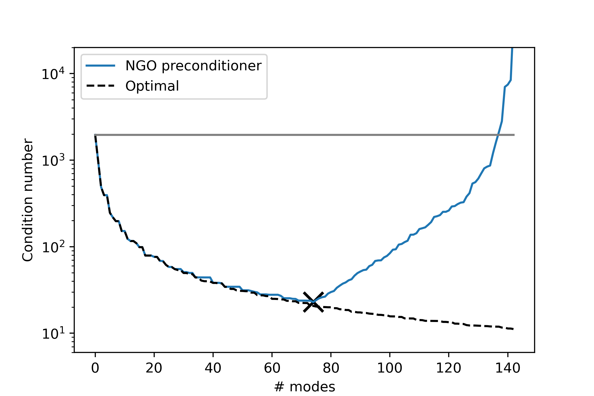
Figure 10 shows the effect of using an NGO as a preconditioner for the finite difference discretisation. The NGO obtains the best preconditioner (smallest condition number) when the $k=74$ dominant SVD modes are used to construct the preconditioner. Note that this is significantly smaller than the total number of basis functions, which is $144$. With 74 modes, the condition number of the linear system decreases from $1959.85$ to $22.93$. The dashed line in the left subfigure shows the optimal condition number for a rank-$k$ preconditioner, which can be computed from the singular values of the original matrix $\mathbf{A}$. This shows that the NGO learns the first 74 singular vectors of the differential operator relatively accurately.

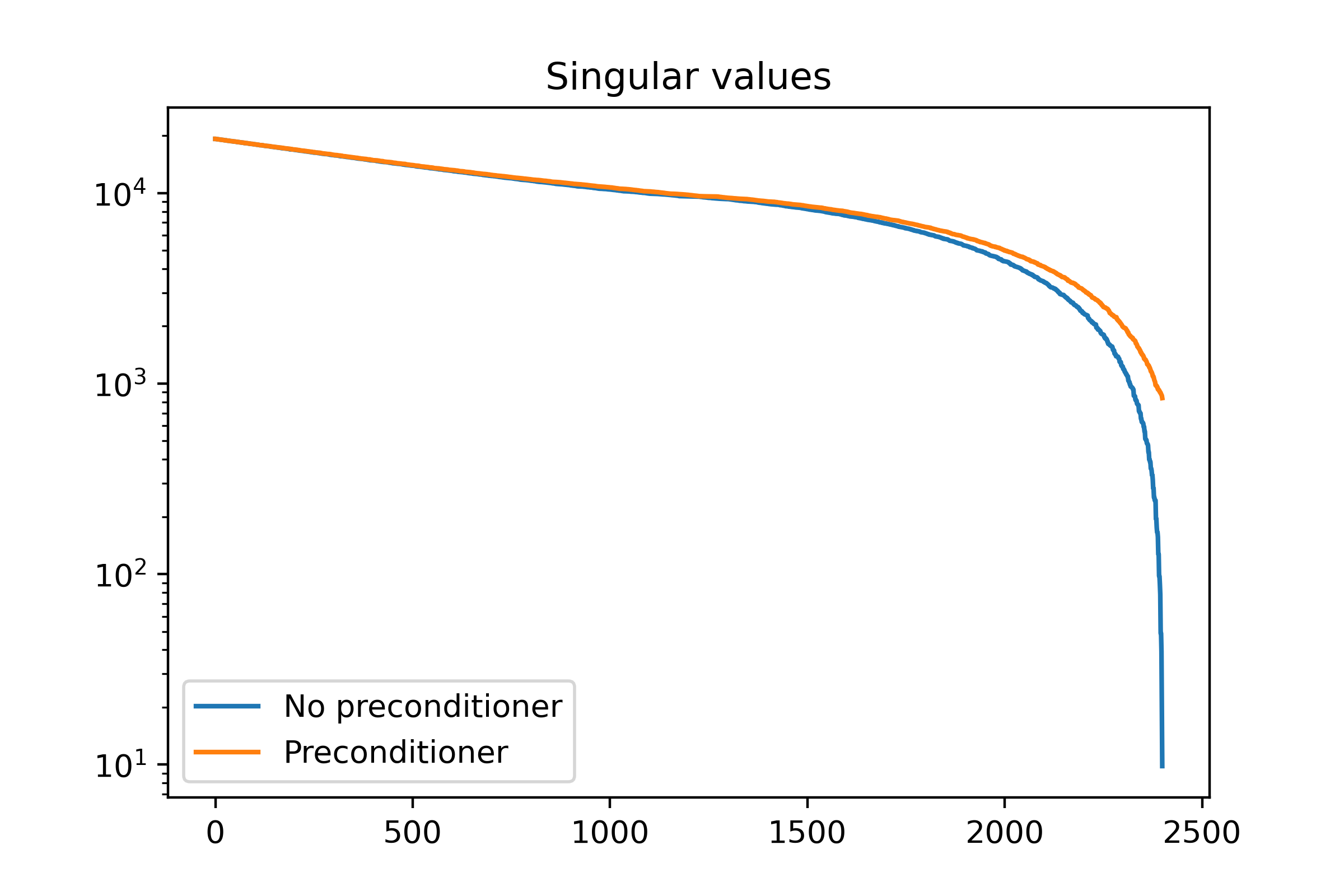
The right plot in Figure 10 shows the singular values of $\mathbf{A}$, as well as the singular values of $\mathbf{PA}$. This shows that:

1. The condition number of $\mathbf{A}$ is indeed large due to a relatively small number of small singular values, which correspond to low frequencies.

2. The preconditioner amplifies these low frequencies, raising their singular values and thereby decreasing the condition number.

Figure 10: Left: the condition number of the preconditioned matrix $\mathbf{AP}$ as a function of the number of modes $k$ included in the preconditioner. The cross indicates the lowest reached condition number, which is achieved with $k=74$. Right: the singular values of the original matrix $\mathbf{A}$ and the optimal (with $k=74$ modes) preconditioned matrix $\mathbf{AP}$.

6 Conclusion

In this manuscript, we have introduced the Neural Green’s Operator, a novel machine learning architecture for learning the solution operator to parametric linear partial differential equations. A key feature of NGOs is that their architecture is derived directly from the Green’s function formulation of the solution operator. On the Darcy flow test problem, the accuracy of NGOs matches that of Fourier Neural Operators and VarMiONs when tested on data that lies in the training distribution. Furthermore, when testing models on finer scale data that does not lie in the training distribution, NGOs consistently outperform all other model architectures that are tested.

We show that the improved generalisation ability of NGOs is the result of two architectural features. Firstly, NGOs are designed for linear PDEs, and are therefore made to include the correct linear structure. This linearity is a strong inductive bias, which cannot easily be implemented in DeepONets and FNOs, since those models do not distinguish linear inputs ($f$ and $\eta$) from non-linear inputs ($\theta$). Secondly, NGOs differ from DeepONets and VarMiONs in that NGOs create a finite-dimensional representation of the input parameters by computing inner products with a set of basis functions, instead of sampling the inputs at a fixed set of sensor nodes. The inner products have the effect of smoothing out higher-frequency components in the inputs, thus making the model less sensitive to the presence of such high-frequency components. Additionally, the inner products allow us to use finer quadrature, allowing for more small scale information to enter the model, without increasing the model size. DeepONets and VarMiONs, which work with samples of the input functions, cannot produce reasonable solutions if the characteristic length scale of the inputs is less than the distance between sensor nodes. Increasing the number of sensor nodes is therefore a requirement to improve generalisation of DeepONets and VarMiONs, but this cannot be done without drastically increasing the number of trainable parameters in those models.

Apart from being an accurate and generalisable surrogate model, the specific structure of NGOs allows them to be used to construct preconditioners for numerical discretisations of PDEs. This ability is demonstrated on a finite difference discretisation, for which the NGO-based preconditioner can decrease the condition number by almost two orders of magnitude. Another advantage of this architecture is that the training and inference performance of NGOs are competitive, in terms of memory usage and measured throughput, to DeepONets, VarMiONs and FNOs.

The results presented here provide a number of directions for future work. The first is the inclusion of more PDEs as test problems, including PDEs with more input functions. Of particular interest is the inclusion of test problems in which the domain $\Omega$ is not kept constant, but is instead treated as an input to the model. Unlike FNOs, the NGO architecture does not depend on a specific shape for the domain, meaning it can be applied to arbitrary geometries directly, i.e. without the need to transform the problem back onto a reference domain as is necessary for FNOs [26]. The second is a more rigorous study of the efficacy of NGOs as preconditioners, including their application as such inside a linear solver such as Conjugate Gradient or GMRES. Thirdly, NGOs can be extended to systems of PDEs (with more than one unknown scalar field), and even to non-linear PDEs by learning a linearisation so that a fixed-point iteration can be applied to the trained NGO.

Appendix A Model architectures

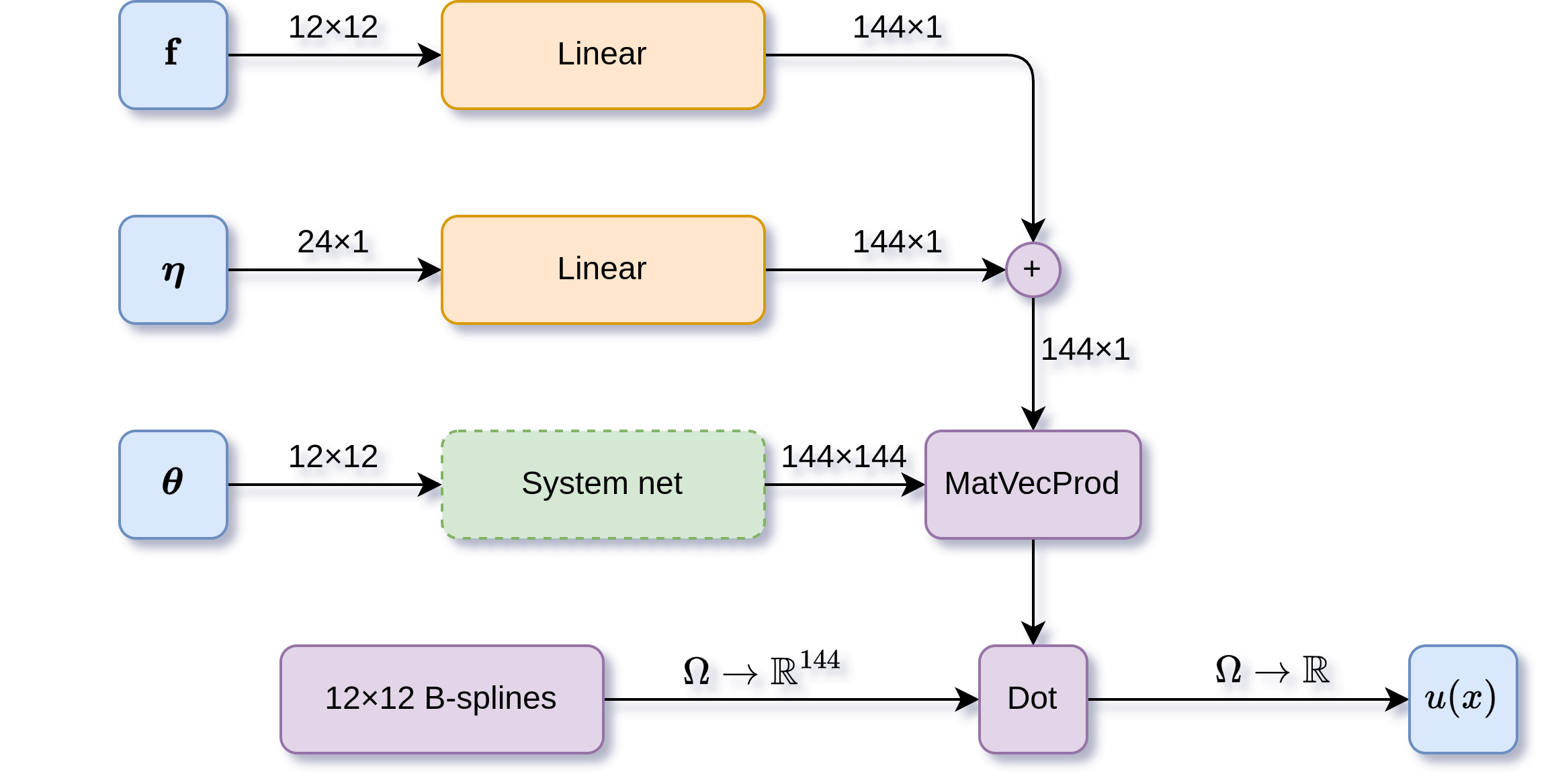
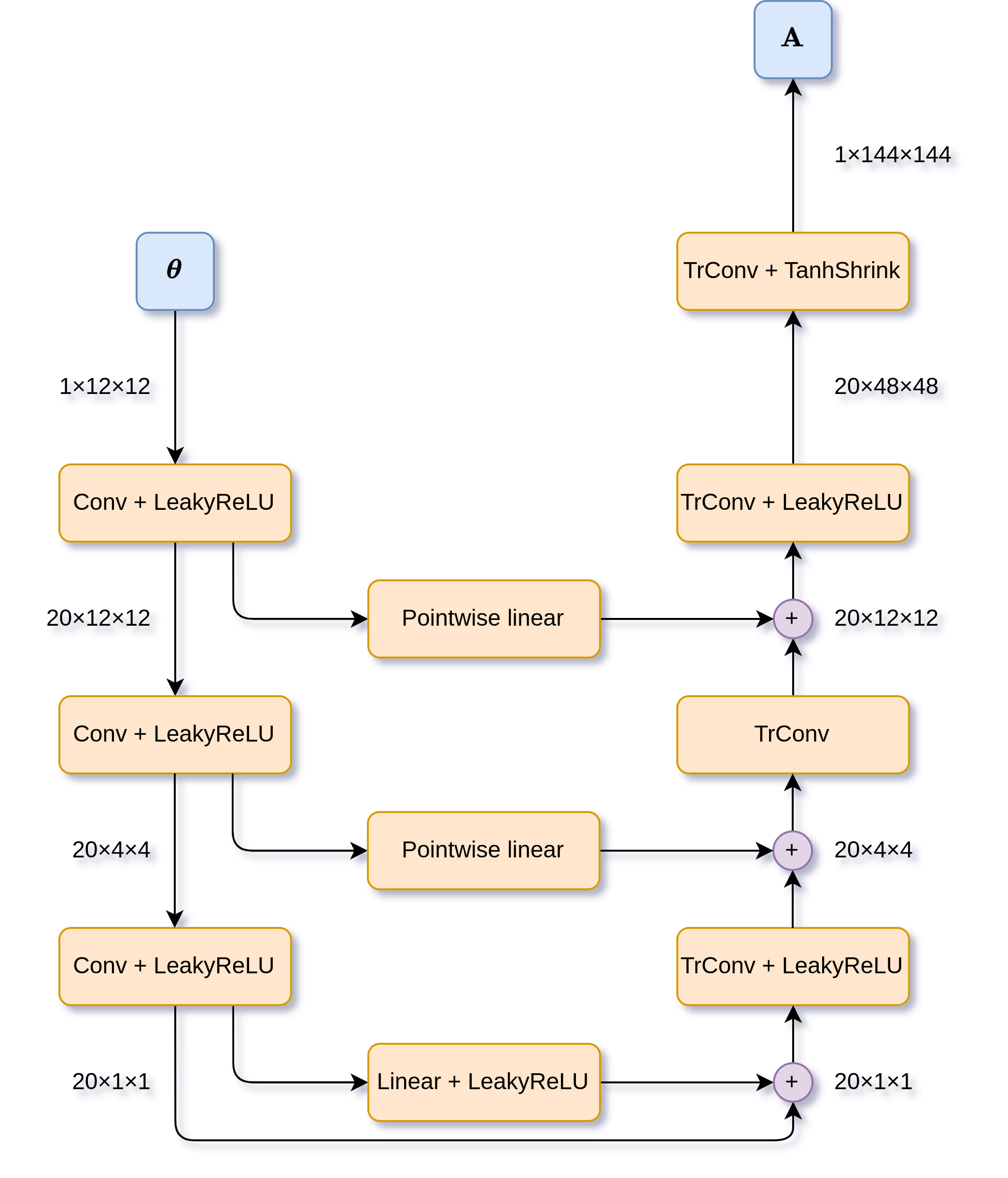
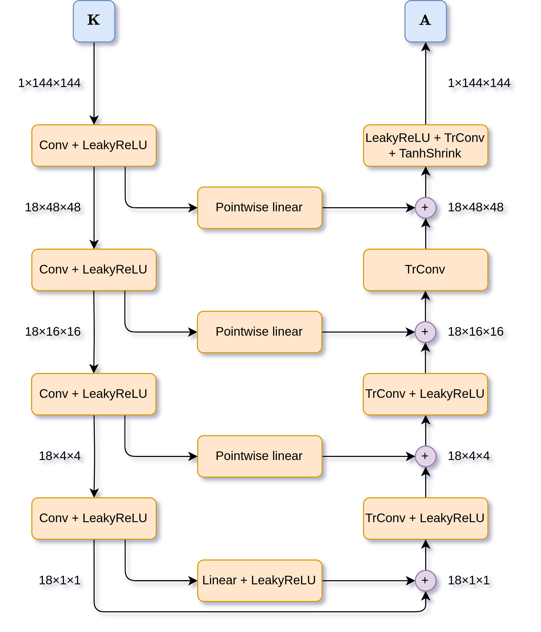
Figure 11 shows the architectures of the DeepONet, FNO, and VarMiON. Figure 12 shows the architectures of the NGOs. The architectures of the system networks for the VarMiON and NGOs are shown in Figure 13. The UNet architectures for the Data-NGO and VarMiON are identical with exception of the number of channels in the hidden layers. This is due to the extra $144\times 144$ linear layer in the VarMiON, which means that the UNet must have fewer parameters in order to keep the total parameter count approximately the same.

Figure 11: From top to bottom: architectures of the DeepONet, FNO, and VarMiON.

Figure 12: Architecture of the model-based NGO (top) and data-based NGO (bottom).

Figure 13: UNet (system) architectures of the VarMiON (top left), Data-NGO (top right), and Model-NGO (middle).

References

- [1] Thomas JR Hughes, Gonzalo R Feijóo, Luca Mazzei, and Jean-Baptiste Quincy. The variational multiscale method—a paradigm for computational mechanics. Computer methods in applied mechanics and engineering, 166(1-2):3–24, 1998.
- [2] Thomas JR Hughes. The finite element method: linear static and dynamic finite element analysis. Courier Corporation, 2012.
- [3] John David Anderson and John Wendt. Computational fluid dynamics, volume 206. Springer, 1995.
- [4] Yuri Bazilevs, Kenji Takizawa, and Tayfun E Tezduyar. Computational fluid-structure interaction: methods and applications. John Wiley & Sons, 2013.
- [5] Yuan-cheng Fung, Pin Tong, and Xiaohong Chen. Classical and computational solid mechanics. World Scientific, 2001.
- [6] Lu Lu, Xuhui Meng, Shengze Cai, Zhiping Mao, Somdatta Goswami, Zhongqiang Zhang, and George Em Karniadakis. A comprehensive and fair comparison of two neural operators (with practical extensions) based on fair data. Computer Methods in Applied Mechanics and Engineering, 393:114778, 2022.
- [7] Kurt Hornik, Maxwell Stinchcombe, and Halbert White. Multilayer feedforward networks are universal approximators. Neural networks, 2(5):359–366, 1989.
- [8] Tianping Chen and Hong Chen. Universal approximation to nonlinear operators by neural networks with arbitrary activation functions and its application to dynamical systems. IEEE transactions on neural networks, 6(4):911–917, 1995.
- [9] Lu Lu, Pengzhan Jin, Guofei Pang, Zhongqiang Zhang, and George Em Karniadakis. Learning nonlinear operators via deeponet based on the universal approximation theorem of operators. Nature machine intelligence, 3(3):218–229, 2021.
- [10] Zongyi Li, Nikola Kovachki, Kamyar Azizzadenesheli, Burigede Liu, Kaushik Bhattacharya, Andrew Stuart, and Anima Anandkumar. Fourier neural operator for parametric partial differential equations. arXiv preprint arXiv:2010.08895, 2020.
- [11] Zongyi Li, Nikola Kovachki, Kamyar Azizzadenesheli, Burigede Liu, Andrew Stuart, Kaushik Bhattacharya, and Anima Anandkumar. Multipole graph neural operator for parametric partial differential equations. Advances in Neural Information Processing Systems, 33:6755–6766, 2020.
- [12] Nikola Kovachki, Zongyi Li, Burigede Liu, Kamyar Azizzadenesheli, Kaushik Bhattacharya, Andrew Stuart, and Anima Anandkumar. Neural operator: Learning maps between function spaces with applications to pdes. Journal of Machine Learning Research, 24(89):1–97, 2023.
- [13] Dmitrii Kochkov, Jamie A Smith, Ayya Alieva, Qing Wang, Michael P Brenner, and Stephan Hoyer. Machine learning–accelerated computational fluid dynamics. Proceedings of the National Academy of Sciences, 118(21):e2101784118, 2021.
- [14] Wang Xiao, Ting Gao, Kai Liu, Jinqiao Duan, and Meng Zhao. Fourier neural operator based fluid-structure interaction for predicting the vesicle dynamics. arXiv preprint arXiv:2401.02311, 2024.
- [15] Salah A Faroughi, Nikhil M Pawar, Célio Fernandes, Maziar Raissi, Subasish Das, Nima K Kalantari, and Seyed Kourosh Mahjour. Physics-guided, physics-informed, and physics-encoded neural networks and operators in scientific computing: Fluid and solid mechanics. Journal of Computing and Information Science in Engineering, 24(4):040802, 2024.
- [16] Xingchen He, Lianshan Yan, Lin Jiang, Anlin Yi, Zhengyu Pu, Youren Yu, Hongwei Chen, Wei Pan, and Bin Luo. Fourier neural operator for accurate optical fiber modeling with low complexity. Journal of Lightwave Technology, 41(8):2301–2311, 2022.
- [17] Daniel Loghin. Green’s functions for preconditioning. 1999.
- [18] Kenneth Franklin Riley, Michael Paul Hobson, and Stephen John Bence. Mathematical methods for physics and engineering: a comprehensive guide. Cambridge university press, 2006.
- [19] Harshwardhan Praveen, Nicolas Boullé, and Christopher Earls. Principled interpolation of green’s functions learned from data. Computer Methods in Applied Mechanics and Engineering, 409:115971, 2023.
- [20] Yuankai Teng, Xiaoping Zhang, Zhu Wang, and Lili Ju. Learning green’s functions of linear reaction-diffusion equations with application to fast numerical solver. In Mathematical and Scientific Machine Learning, pages 1–16. PMLR, 2022.
- [21] Rixi Peng, Juncheng Dong, Jordan Malof, Willie J Padilla, and Vahid Tarokh. Deep generalized green’s functions. arXiv preprint arXiv:2306.02925, 2023.
- [22] Craig R Gin, Daniel E Shea, Steven L Brunton, and J Nathan Kutz. Deepgreen: deep learning of green’s functions for nonlinear boundary value problems. Scientific reports, 11(1):21614, 2021.
- [23] Dhruv Patel, Deep Ray, Michael RA Abdelmalik, Thomas JR Hughes, and Assad A Oberai. Variationally mimetic operator networks. Computer Methods in Applied Mechanics and Engineering, 419:116536, 2024.
- [24] Joost Simon Boudewijn van Zwieten, Gerrit Johannes van Zwieten, and Wijnand Hoitinga. Nutils, November 2023.
- [25] Erisa Hasani and Rachel A Ward. Generating synthetic data for neural operators. arXiv preprint arXiv:2401.02398, 2024.
- [26] Zongyi Li, Daniel Zhengyu Huang, Burigede Liu, and Anima Anandkumar. Fourier neural operator with learned deformations for pdes on general geometries. Journal of Machine Learning Research, 24(388):1–26, 2023.