Non-uniformity is All You Need: Efficient and Timely Encrypted Traffic Classification With ECHO

Abstract.

With 95% of Internet traffic now encrypted, an effective approach to classifying this traffic is crucial for network security and management. This paper introduces ECHO—a novel optimization process for ML/DL-based encrypted traffic classification. ECHO targets both classification time and memory utilization and incorporates two innovative techniques.

The first component, HO (Hyperparameter Optimization of binnings), aims at creating efficient traffic representations. While previous research often uses representations that map packet sizes and packet arrival times to fixed-sized bins, we show that non-uniform binnings are significantly more efficient. These non-uniform binnings are derived by employing a hyperparameter optimization algorithm in the training stage. HO significantly improves accuracy given a required representation size, or, equivalently, achieves comparable accuracy using smaller representations.

Then, we introduce EC (Early Classification of traffic), which enables faster classification using a cascade of classifiers adapted for different exit times, where classification is based on the level of confidence. EC reduces the average classification latency by up to 90%. Remarkably, this method not only maintains classification accuracy but also, in certain cases, improves it.

Using three publicly available datasets, we demonstrate that the combined method, Early Classification with Hyperparameter Optimization (ECHO), leads to a significant improvement in classification efficiency.

1. Introduction

Internet traffic classification is a critical challenge in network management, security, and optimization. Traffic classification can be used for application identification (Shapira and Shavitt, 2019), traffic categorization (Draper-Gil et al., 2016; Akbari et al., 2021), identifying encryption methods like VPN or Tor (Lashkari et al., 2017), detecting malicious activities such as Distributed Denial of Service (DDoS) attacks (Wang et al., 2018; Sharafaldin et al., 2018; Bronzino et al., 2021), and device fingerprinting (Engelberg and Wool, 2021).

In the past, classification methods such as port-based classification (using the predefined ports associated with specific services or applications) or signature-based Deep Packet Inspection (DPI) were considered sufficient (cf. (Finsterbusch et al., 2014; Aceto et al., 2010)).

However, the use of random ports, shared port usage between applications, and most importantly, the widespread adoption of encryption protocols—such as TLS/SSL encryption, VPN tunneling, and anonymous communication technologies (e.g. Tor (Enghardt et al., 2020; Moore and Papagiannaki, 2005))—have significantly hindered the ability to inspect and classify traffic based on these approaches.

Thus, new approaches were introduced to deal with encrypted traffic, mostly focused on extracting features from each flow (namely, the flow representation) and applying Machine Learning (ML) or Deep Learning (DL) methods to classify it. As most data is obfuscated, these methods typically use as input only the size of packets, their inter-arrival times, and their direction.

While many proposed methods claim high accuracy in classification, implementing these approaches in real-life scenarios can be challenging due to the large volume of traffic (namely, hundreds of Gb/s in large ISPs) and the huge number of concurrent connections (namely, millions of new connection per second). Thus, storing flow content, headers, or representations requires considerable memory resources. Moreover, the deployment of DL or large ML models demands significant computational power.

To reduce both memory and compute, flow representations often aggregate values, and each packet size (or arrival time) is mapped to a bin. The representation then typically holds a counter for each bin, tracking the number of packets whose size (or arrival time) falls within that bin. This is most commonly done in a uniform manner with all bins being the same size. However, such coarse-grained uniform binning might fail to capture subtle nuances in traffic patterns.

This paper first explores non-uniform binnings, as real-world traffic data often exhibit non-uniform patterns. We introduce variable-sized bins, each representing an interval of values, allowing for a more fine-grained and adaptive approach to capturing non-uniform traffic patterns, with smaller representations. Examples of uniform and non-uniform binnings of the packet size distribution for a sampled flow are shown in Figure 1.

(a) A uniform binning

(b) A non-uniform binning

Figure 1. A uniform and a non-uniform binning of the packet size distribution of the same example flow. Vertical dotted black lines mark the boundaries of the 5 selected bins. By using non-uniform representations, we can capture more fine-grained details of the flow.

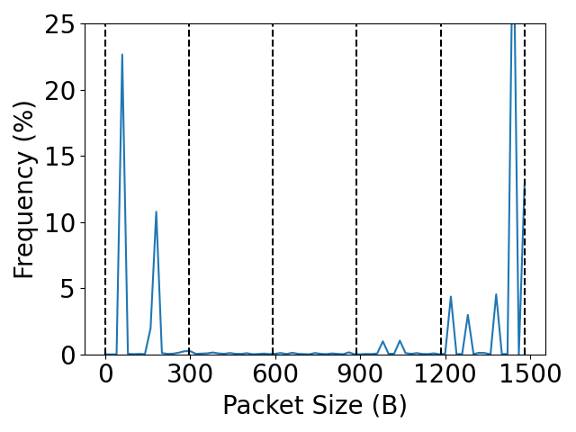
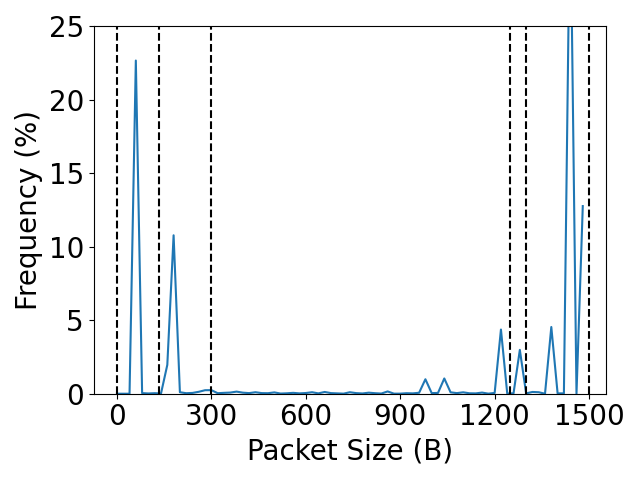
The selection of bins can be approached either manually or algorithmically. However, as there are usually multiple classes and a significant number of flows, manual selection of bin boundaries may be impractical and imprecise. Employing statistical methods for bin selection (or selecting only a subset of the available features) might introduce an improvement over uniform binning. Nonetheless, model-agnostic techniques might fail to capture complex relations between features. Therefore, we propose a flexible, data-aware and model-aware approach.

Innovatively, to determine the binning, we employ Hyperparameter Optimization (HO). In this method, we apply Bayesian optimization methods to optimize the bin boundaries in the training stage. Our results show that our HO method outperforms other optimization methods, such as feature selection and statistical bin selection across all classification tasks, by up to 15% in accuracy. The full description of the proposed method is in Section 4.

Another aspect we optimize is the collection time; that is, the time required for collecting properties from the flow until a classification is made. Many existing approaches classify flows only after they end, after a predefined amount of time has elapsed, or after a specific number of packets have been received. Typically, the collection time is orders of magnitude longer than the inference time, thus dominating the overall classification time.

We notice that some flows contain indicative features useful for classification at an early stage, while others require more time for accurate classification. Thus, we introduce Early Classification (EC), a novel setup performing classification in multiple exit times and making a final prediction only upon reaching a certain level of confidence in the classification. Our system is adaptive, classifying some flows at earlier stages, and waiting longer for flows with low confidence in earlier classifications. As our system may invoke multiple classifiers for each flow, we need to create multiple different representations, which might be prohibitive when the number of concurrent flows is large. Consequently, we present a method for creating additive traffic representations, such that the process of updating the representations between classifiers does not incur any additional memory requirements. Additionally, we propose a method that creates tradeoffs between accuracy and collection time, allowing users to tailor these parameters to their specific requirements. The EC setup is presented in Section 5.

In conclusion, this work makes two significant contributions. First, we introduce HO. Our exploration showcases the effectiveness of this strategy, which allows us to improve the classification accuracy by 5%–20% in multiple classification tasks, or, alternatively, reduce memory requirements and computational overheads (as smaller classifiers are required) by 90%.

Our second contribution is by presenting EC, a novel method enabling early traffic classification with an adaptive classification approach. Using this method, the required time for classification can be reduced by up to an order of magnitude, with minimal decline in accuracy, and possibly even an improvement.

Finally, we combine the two methods to create ECHO classifiers, achieving both an accuracy boost of up to 10%, and a reduction in the average collection time by 95%.

The two suggested techniques can be adapted easily to many existing approaches for traffic classification, substantially enhancing their performance.

The rest of this paper is organized as follows: We discuss related work in Section 2. Section 3 explains the networking model and defines the problem of encrypted traffic classification. Section 4 introduces HO, where Bayesian hyperparameter optimization yields non-uniform binnings for packet sizes and arrival times. Section 5 outlines the Early Classification (EC) setup. Subsequently, in Section 6, we present the combined ECHO approach. Finally, Section 7 presents the evaluation results based on three publicly-available datasets, followed by conclusions drawn in Section 8. Note that additional information, including details about our datasets and comparison between different models and representations, is given in the appendices.

2. Related Work

Encrypted traffic classification has been extensively studied in recent years (cf. (Zhao et al., 2021; Salman et al., 2020) and references therein). Modern classifiers predominantly utilize ML or DL techniques over representations created from the encrypted traffic. Commonly used representations are statistical features extracted from the traffic (Williams et al., 2006; Draper-Gil et al., 2016; Lashkari et al., 2017; Anderson and McGrew, 2017), time-series of the first packets of the flow(Bernaille et al., 2006a; Yang et al., 2021), and distributional representations, which include dist (Engelberg and Wool, 2021)—2 pairs of distribution vectors representing packet sizes and arrival times per traffic direction—and flowpic (Horowicz et al., 2022; Shapira and Shavitt, 2019; Finamore et al., 2023)—a two dimensional representation where each element in the matrix captures the number of packet of a certain size arriving at a certain time. Notice that distributional representations often outperform other representations (Finamore et al., 2023) (see further comparison results in Appendix B), and therefore, are employed in this paper.

Many methods and representations require substantial memory and compute resources, which makes them impractical for large networks.

To mitigate the memory and compute requirements, some works (e.g.,  (van Ede et al., 2020; Moore and Zuev, 2005; Ertam and Avcı, 2017; Shafiq et al., 2018; Williams et al., 2006; Fahad et al., 2013; Bronzino et al., 2021; Holland et al., 2021)), have shown how to extract certain features (e.g., flow statistics) from the traffic, or reduce feature dimensionality using feature selection.

Non-uniform binnings (as we suggest in this work) were rarely considered in the context of flow representations. There are two notable works in this area. Barradas et al. (Barradas et al., 2021) have suggested an optimization process that consists of creating uniform binning for packet size distribution and pruning bins using feature selection methods, where the final selection of features is a subset of the original uniform bins. Garcia et al. (Garcia and Korhonen, 2018) have proposed a statistical algorithm based on the Kolmogorov-Smirnov statistical test for selecting histogram bins, aiming at maximizing the separation between classes (measured using the Jensen-Shanon Distance).

Our research focuses on the introduction of non-uniform binnings derived by a Bayesian hyperparameter optimization process. We note that in the field of traffic classification, most previous literature regarding Bayesian hyperparameter optimization is focused on selecting hyperparameters for classifiers (Bergstra et al., 2011, 2013), but not for flow representations. HO, our strategy for creating non-uniform representations, outperforms all previously suggested optimization methods in all explored classification tasks, and can be plugged into many of the previous works to enhance their performance and reduce their memory footprint, as detailed in Section 4.

As for early classification, some works have suggested using the first few packets of the flow for early classification of flows (Bernaille et al., 2006b, c, a; Yang et al., 2021; Wang et al., 2017b; Lotfollahi et al., 2017; Lopez-Martin et al., 2017; Liu et al., 2019; Zou et al., 2018). While for some classification tasks, the first few packets of a connection suffice, this is not always the case and can lead to less accurate classification (Finamore et al., 2023), this trend is also observable in our experiments (Appendix B).

A first step towards early classification was suggested in  (Wang et al., 2023; Sivanathan et al., 2019), where two classifiers are used: the first classifier is based on simpler classification rules, while the second classifier employs more complex rules or a larger model, allowing for more adaptive classification schemes. To the best of our knowledge, in the context of encrypted traffic classification, no extensive research was conducted on building confidence-based classifiers, where a classification is made only after reaching a threshold of certainty.

3. Problem Statement

We first describe our networking model and define precisely the problem at hand.

Data is transmitted over the network from a source to a destination as a flow (namely, a timestamped sequence of packets) over communication links. Typically, many flows share the same communication link. Thus, when observing a communication link, we first need to map the packets to their corresponding flows.

We note that flows are commonly defined by a five-tuple (namely, the following five header fields in an IP packet: source and destination IP addresses, source and destination ports, and protocol) (Nguyen and Armitage, 2008; Williams et al., 2006). However, this definition is not rigid and can be seamlessly modified to meet different settings or requirements (e.g., in case parts of the five-tuple will be obfuscated in the future or to address a different classification task).

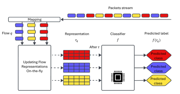
This work focuses on classifying flows that traverse the network. Thus, when a flow (with identifier $q$) is initiated or requires classification, a flow representation $r_{q}$ is generated to capture relevant properties of $q$. Since encryption techniques obfuscate most features, we assume only packet sizes, arrival times, and packet directions are available. We aim to classify a large number (namely, millions) of flows simultaneously, implying that, at any given time, many flow representations are being collected and stored in the system.

Flow information is collected for a predefined time $\tau$, where the representation $r_{q}$ is built on the fly. Then, $r_{q}$ is passed to a classifier $f$, which predicts the label $f(r_{q})$ of flow $q$. Upon classification, the appropriate actions may be taken based on the predicted class, such as generating an alert, adding the information to a database, or blocking certain activities. Subsequently, the flow is marked as classified. Alternatively, time-limited classifications can be employed, where the classification remains valid for a specific duration, after which the flow should be reclassified to ensure up-to-date classification results. Figure 2 illustrates the collection and classification process.

Figure 2. The key stages in the classification process. Packets are mapped by their flow (the color), and the flow representations are updated accordingly. After a predefined timeout, the flow representation is passed into a classifier to predict the class of the flow (e.g., the used application). Arrows represent the flow of data between the stages, whereas dotted arrows indicate memory access.

4. Hyperparameter Optimization (HO) of Binnings

In this section, we present HO, a novel strategy to create non-uniform binnings that enable efficient classification. We have explored both non-uniformity in the packet size distribution vector and the arrival-time distribution vector.

Binning consists of reducing the granularity of the representation such that each original value is mapped to a bin. Each bin represents an interval of the original values. Formally, a uniform representation of size $N$ for values in $[0,x)$ represents the data in $N$ bins, where bin $i\in\{1,\ldots,N\}$ is for values in $[\frac{(i-1)\cdot x}{N},\frac{i\cdot x}{N})$. A non-uniform $N$-bin representation has additional degrees of freedom to choose the boundaries by defining a vector

$$B=[b_{0},\ldots,b_{N}],$$

such that $0=b_{0}<b_{1}<\ldots<b_{N-1}<b_{N}=x$. In such a representation, bin $i\in\{1,\ldots,N\}$ is for values in $[b_{i-1},b_{i})$. In general, we examine two additional properties of binnings: data-aware and model-aware binnings.

A binning is data-aware if, in the creation process, it takes properties of the traffic into account. A simple example of data-aware binning is to employ Feature Selection methods and decide not to store some of the (fixed-sized) bins, based on the data (Barradas et al., 2021).

A more sophisticated data-aware binning is to use Statistical methods to select variable-sized bins (represented as a vector $B$) that create a separation between the distributions of the different classes of the data. Inspired by (Garcia and Korhonen, 2018), we use a multiclass version of the Jensen-Shanon distance metric (Lin, 1991), where classes are compared in an one-vs-all manner.

A model-aware binning, which we are first to propose, corresponds to the specific classifier that will eventually use the representations for classification. This approach allows us to tune the representation by the anticipated performance of the final model, distinguishing it from all other binning operations (see Table 1).

Orthogonal to the information available to the binning process is the way the different elements in $B$ are selected, where we distinguish between two approaches. The naive greedy approach (as used, for example, in (Garcia and Korhonen, 2018)) iteratively selects a single bin boundary, maximizing the objective function given previous selections.

Table 1. The different parameters observable by the representation-optimization process

	Data-aware	Variable Sized Bins	Model-aware
Uniform	✗	✗	✗
Feature Selection	✓	✗	✗
Statistical	✓	✓	✗
HO	✓	✓	✓

HO, on the other hand, employs a hyperparameter optimization algorithm for binning selection. Hyperparameter optimization, in general, refers to the process of finding the best combination of hyperparameters (configuration settings that are not learned in the training stage, but rather set before training the classifier) for a given classifier. In our context, the hyperparameters are the selected bins for the representation, the search space includes all possible combinations of bin boundaries, and the objective we aim to maximize in the Bayesian process is the accuracy of a trained model over the validation set. While many hyperparameter optimization approaches exist, we focus on the Tree Parzen Estimators (TPE) method, as it shows superiority over other approaches in past experiments (Bergstra et al., 2011, 2013).

We note that, unlike (Garcia and Korhonen, 2018), we apply TPE also on the Statistical approach, where the objective function corresponds to the Jensen-Shannon distance derived from the possible binnings. While such bin selection is better than the greedy approach, it is still inferior to HO as the Statistical approach is not model-aware.

For the experiments in this work, we use $k$-fold cross-validation (KFCV) (Kohavi, 1995). Therefore, to validate the TPE process, we use nested cross-validation (NCV) (Cawley and Talbot, 2010), an extension of KFCV for hyperparameter optimization. NCV consists of an outer loop for standard KFCV, selecting training and test sets in each iteration. In the inner loop, we use the training data to iteratively select optimal hyperparameters through another KFCV process. We use $k=5$ in both the outer and inner loops, implying that for each evaluation in the inner loop, $64\%$ of the flows are used for training, $16\%$ for validating the hyperparameters by calculating the objective function, and $20\%$ for testing (in the outer loop). It is important to note that different iterations of the outer loop might yield different hyperparameter values.

Notice that in our settings, the optimization process is done offline on labeled data, and therefore, has fewer constraints regarding computational power or latency.

Once the optimization process finishes and an optimal result is achieved, the real-time classifier is adapted and uses the optimal hyperparameters (namely, the bin boundaries) achieved by the offline optimizer.

After selecting the bin boundaries, to create our representations without any computational overhead, we create a mapping, using a small direct-access array of size $x$, between every possible packet size (or discretized arrival time) to its bin index; this implies that the process of building our representations (which is done online, packet by packet) does not incur additional computations (only one memory access).

To capture changes in traffic patterns or in the underlying applications, we propose to run HO periodically, upon degradation of accuracy, or manually if a change in the network condition is known. The process should run in the background without interfering with ongoing classifications.

The results achieved using HO, as well as a comprehensive comparison to the alternative methods, are shown in Section 7.1.

5. Early Classification (EC) of Traffic

In this section, we will describe the system setup enabling early traffic classification. EC not only improves the Quality of Service (QoS) and the network security but also saves memory requirements, as flow representations are stored for shorter periods.

This method is based on the assumption that some flows have indicative features at earlier stages and there is no need to wait for a long time to reach an accurate classification. Therefore, in the proposed setup, classification occurs upon reaching a sufficient confidence level, without the need to wait several seconds and collect the full traffic representation. For assessing models’ confidence, we exploit the fact that many classifiers output the predicted results as a vector $f^{\prime}(r)=u$, where $u$ consists of the predicted probability that a sample is in each class. The predicted class for some sample is then $f(r)=\arg\max_{i=1}^{C}f^{\prime}(r)$. For EC, we define the confidence of the classification, denoted by $\beta_{q}$, as the maximal argument in the resulting vector; namely,

$$\beta_{q}=\max_{i=1}^{C}f^{\prime}(r_{q}).$$

We note that this approach can be replaced with several different methods for assessing model confidence, as discussed by (LEI, 2014).

The core idea behind EC is that classification occurs in multiple exit times $\tau_{1},\ldots,\tau_{max}$, and the final prediction is made when the confidence value exceeds a predefined threshold $\beta$, or if the maximal time $\tau_{max}$ has elapsed.

For employing an efficient EC system, we first train (offline) different classifiers $f_{1},\ldots,f_{max}$ for multiple durations in a logarithmic scale (namely, $\tau_{i+1}=2\cdot\tau_{i}$) up to the maximal duration $\tau_{max}$ selected for the classification task.

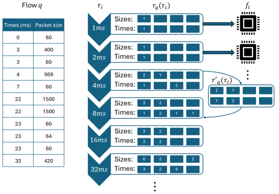
In the online phase, we iteratively build the traffic representations. First, we build the distribution vectors with regard to the first exit time and feed it into the first classifier. If the sample is not classified with sufficient confidence, we keep the packet-sizes distribution vector unchanged and keep collecting packets to it. For the arrival-times distribution vector, in order to adjust the representation to the next classifier, we first merge each bin $2i-1$ with its adjacent bin $2i$, leaving the second half of each vector empty. Then, we count arriving packets into the second halves of these vectors, where each bin corresponds to the time that passed since the beginning of the collection process. Formally, for $d({\tau_{i}})$ being a distribution vector of the arrival times for the exit time $\tau_{i}$ (for a single side of the traffic), the values in the updated vector $d({\tau_{i+1}})$ for the next exit time will be:

$$d({\tau_{i+1}})_{j}=\begin{cases}d({\tau_{i}})_{2j-1}+d({\tau_{i}})_{2j}&:j\leq\frac{N}{2}\\ \#(\text{packets in }[\frac{j-1}{N}\cdot 2\tau_{i},\frac{j}{N}\cdot 2\tau_{i}))&:\text{else}\\ \end{cases}.$$

Using this method, no additional memory is required, and the representations are built and adjusted to the different classifiers on the fly. This process is illustrated in Figure 3.

Figure 3. An illustration of the iterative process of creating the representations for the different time scopes. On the left is an example flow with the arrival times and packet sizes of the first 11 packets. The packet-size boundaries vector is $[0,375,750,1125,1500]$, the arrival time boundaries vector is dependant on the time scope: $[0,\frac{\tau_{i}}{4},\frac{\tau_{i}}{2},\frac{3\tau_{i}}{4},\tau_{i}]$. $r^{{}^{\prime}}_{q}(\tau_{i})$ is the updated representation before adding the packets in the next time interval.

To minimize the negative effect this process might have on classification, we select the confidence threshold $\beta$ as the accuracy of a baseline model that classifies all flow after $\tau_{max}$.

Surprisingly, this scheme not only reduces the average classification time but in some cases also improves the overall classification accuracy. This might occur due to the multiple exit options, allowing the models to identify timely behaviors that are more discernible in earlier classifiers.

Additionally, we explore the tradeoffs between the average collection time and the overall classification accuracy by altering the classification threshold $\beta$ with small $\alpha$ values, making early predictions if the confidence is higher than $\beta-\alpha$.

As shown in Appendix B.2, the classification throughput highly depends on the selected classifier and the representation size. Therefore, if EC is deployed on edge devices, at high network rates, or if a strong classifier is selected, there will be a tradeoff between the ability to perform early classification and the rate of classification, as this method requires (possibly) employing multiple classifiers on each flow until it reaches the final prediction. Additionally, as the collection time is significantly higher than the inference time of our classifiers, we neglect the inference time in these comparisons. .

The results exploring EC setups are shown in Section 7.2.

6. Early Classification with Hyperparameter Optimization (ECHO)

As we observed that HO improves the performance of models, we wish to create those representations for EC setups as well. For the packet-size distribution vector, we adopt the non-uniform bins of an optimized HO model (a single binning for all classifiers). However, as the arrival time distribution vector are updated in a particular way between EC classifiers (recall Figure 3), customized arrival-times bins cannot be used. The EC setup employing HO on the packet size dimension with uniform time bins is denoted by ECHO.

Yet, we do propose a non-uniform alternative for the arrival time bins, while still maintaining the ability to update the representations in real-time. In this alternative setup, denoted by EC Log, we will use logarithmic bins, that is, for every exit time $\tau_{i}$ and $N$ bins with boundaries $B=[b_{0},\ldots,b_{N}]$, where $b_{0}=0s,\>b_{N}=\tau_{i}$, and the other boundaries ($0<j<N$):

$$b_{j}={\tau_{i}}\cdot{2^{-j}}.$$

Using this selection, if the different exit times are defined logarithmically ($\tau_{i+1}=2\cdot\tau_{i}$), to update the arrival-times vector distribution we simply sum the two values with the smallest indexes, and shift all values one index below. Formally, for $d({\tau_{i}})$ being a single distribution vector of arrival times created at time ${\tau_{i}}$, $d({\tau_{i+1}})$ will be the updated vector for the next classifier:

$$d({\tau_{i+1}})_{j}=\begin{cases}d({\tau_{i}})_{1}+d({\tau_{i}})_{2}&:j=1\\ \#(\text{packets in }[\tau_{i},\tau_{i+1}))&:j=N\\ d({\tau_{i}})_{j-1}&:\text{else}\\ \end{cases}.$$

In Section 7.3, we have evaluated different selections of packet-size bins for the ECHO setup, and explored the proposed method for the logarithmic arrival-times bins (EC Log).

7. Experimental Results

In this section, we provide experimental results investigating the HO strategy for creating efficient traffic representations (Section 4), the EC method for timely traffic classification (Section 5) and the ECHO approach that combines the two strategies (Section 6). We also demonstrate their superiority over alternatives that were previously proposed in the literature.

Our results are structured as follows: First, we examine the effectiveness of HO in traffic classification (Section 7.1). Here, we analyze how the representations created using HO impact classification accuracy and memory utilization. Our investigation highlights the advantages of HO compared to traditional uniform binning and alternative approaches, and provides in-depth insights into the reasons behind the success of the proposed method.

Section 7.2 explores EC methods and how they affect the accuracy and reduce the average collection time of the system.

Finally, we combine the HO method with EC to create efficient classifiers, with high accuracy and with minimal time required for classification (Section 7.3).

In this work, we use the Logistic Regression ($LR$) (Pearl and Reed, 1920) classifier for building the models. $LR$ classifiers offer the highest classification throughput compared to other explored classifiers (a detailed comparison in Appendix B), therefore enabling real-time classification for large volumes of traffic. However, we note that in our experiments, similar trends were observed for different ML and DL classifiers.

We use three publicly-available datasets (Rezaei and Liu, 2020; Draper-Gil et al., 2016; Lashkari et al., 2017; Naas and Fesl, 2023), where classification tasks include application identification (e.g., distinguishing between YouTube and Google Music), encryption identification (e.g., distinguishing between different types of VPN), and traffic categorization (e.g. distinguishing between video and VoIP). The different classification tasks we tackle are presented in Table 2, and a thorough description of the datasets, including our preprocessing stage, is in Appendix A.

It is important to note that our preprocessing ensures that the datasets are balanced across all classification tasks, and the difference between accuracy (percentage of correctly classified samples over the test set) and alternative utility metrics (e.g. f1 score, precision, recall) is negligible. Consequently, we evaluate our models and representations based solely on the achieved accuracy using $k$-fold Cross Validation (KFCV) (Kohavi, 1995) with $k=5$.

Table 2. Different classification tasks we explore. Classification task types are denoted “Apps” for application identification, “Encryption” for encryption identification, and “Categories” for traffic categorization. Additional details appear in Appendix A.

Dataset Name	Task Name	# Classes	Type
Quic (Rezaei and Liu, 2020)	Quic Applications	5	Apps
ISCX combined (Draper-Gil et al., 2016; Lashkari et al., 2017)	ISCX Applications	4	Apps
	ISCX Encryption	3	Encryption
	ISCX Categories	4	Categories
VPN Services (Naas and Fesl, 2023)	VPN Services	6	Encryption
	Streaming or Not	2	Categories

7.1. Hyperparameter Optimization (HO) of Binnings

As observed in our experiments, larger representations improve classification accuracy, but come at the cost of a higher memory footprint and usually more computational requirements.

We compare several methods for selecting binnings over the packet size dimension, including our suggested novel strategy:

Uniform.:

All bins are of equal size; namely, $b_{i}=\frac{i\cdot x}{S}$, where $S$ is the number of bins.

Feature Selection.:

Inspired by (Barradas et al., 2021), we employ feature-selection methods on larger uniform representations, to create a smaller pruned representation. Given the required number of bins $N$, we apply feature selection on multiple uniform representations with different original sizes: $N^{\prime}\in\{10,20,50,100,200,500,1500\},$ and select the model with the highest achieved accuracy. This representation still uses fixed-size bins, however, it is data-aware and selects features with respect to their statistical significance.

Statistical.:

As explained in Section 4, and inspired by (Garcia and Korhonen, 2018), we use the TPE method for optimization of binning, where the objective function is to maximize a multiclass version of the Jensen-Shanon distance metric (Lin, 1991). This method maximizes the statistical separation between the different classes independently of the selected classifier.

HO Sizes.:

Our novel strategy employed on the packet size distribution, using the TPE method with the objective being the accuracy of a trained model, as explained in detail in Section 4.

(a) Quic Applications

(b) ISCX Applications

(c) ISCX Encryption

(d) ISCX Categories

(e) VPN Services

(f) Streaming or Not

Figure 4. Accuracy as a function of the number of bins, for different binning strategies on the packet size dimension. The time dimension binning is uniform in all experiments.

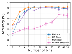
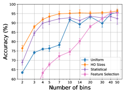
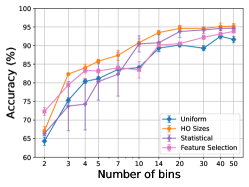
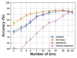
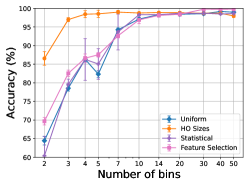
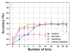
Throughout all our experiments, we set the number of iterations of the TPE method to 200, as we observed convergence in this iterative process. Note that we have also explored greedy sampling methods for hyperparameter selection, where we progressively built the hyperparameter configuration by selecting the option in each subsequent bin that maximized the objective function given the previously chosen options. However, as greedy selection methods do not have as many degrees of freedom, and showed no noticeable advantage over the TPE method, we focus our discussion here on the TPE.

The results are shown in Figure 4. Evidently, the HO Sizes approach is able to capture the nuances and patterns in smaller representations, leading to improved classification accuracy throughout all classification tasks. Additionally, statistical optimization (Statistical) shows an advantage over uniform representations; however, this trend is not consistent for all tasks and sizes. Finally, the Feature Selection method introduces a degradation in accuracy compared to uniform representations. This might be caused by the loss of information in the feature selection process, in the inherent limitation of selecting only sampled features for a single uniform representation (of larger size).

(a) Quic Applications

(b) ISCX Applications

(c) ISCX Encryption

(d) ISCX Categories

(e) VPN Services

(f) Streaming or Not

Figure 5. Accuracy as a function of the number of bins, comparing HO on the different dimensions, as well as on both dimensions.

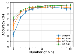
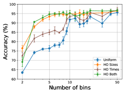
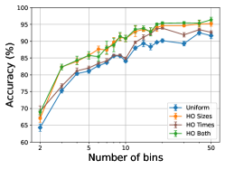
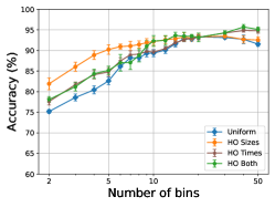
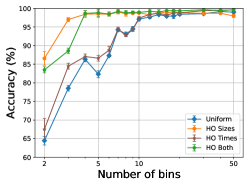
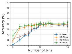
We note that introducing non-uniformity in the packet sizes dimension leads to a significant enhancement in the model’s accuracy, particularly evident when employing the HO Sizes approach. We further explore non-uniformity by introducing non-uniformity in the arrival-times dimension. We compare the following representations: Uniform representations, HO Sizes - that use non-uniform bins for the sizes dimension and uniform bins for the arrival-times dimension (as in Figure 4), HO Times - that use non-uniform bins for the arrival time dimension and uniform bins for the sizes dimension, and HO Both that include optimized binning for both dimensions (with different parameters for each dimension). Results are shown in Figure 5. We see that by itself, non-uniformity in the arrival-times dimension shows some advantage over uniform representations. However, this improvement is limited, and when combined with non-uniformity in the packet-sizes dimension, there is little to no advantage in model accuracy compared to HO Sizes.

7.1.1. Explainability

An important property of our binning strategy is its explainability. This is done by looking at the distribution of packet sizes (or arrival times) for each class, and observing what information is given by the new bin boundaries. For example, for the VPN Services task over 5 bins, Figure 6 depicts the selected bin boundaries of one of the runs of HO Sizes, along with the packet sizes distribution of each class. It is easy to see that bin boundaries are correlated to the data distribution. Specifically, notice that one of the boundaries is at 168 bytes. In retrospect, this appears to distinguish between typical SSTP packets and typical OpenVPN packets. Similarly, the bin boundary of 76 bytes appears to distinguish between L2TP IPsec traffic (which has many smaller packets) and WireGuard traffic (with bigger packets).

Figure 6. (a) The entire packet sizes distribution of the VPN dataset with respect to VPN labels; (b) The histogram zoomed in a specific range with the bin boundaries selected by the HO Sizes strategy (for the VPN Services classification task with 5 bins) marked in black. We can see how the selection of bins correlates to the discriminative features of some classes.

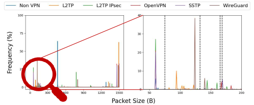
These boundaries demonstrate the strength of the HO approach, as coarse-grained uniform representations commonly group these values together resulting in misclassifications; for example, Figure 7 shows a confusion matrix of a classifier using coarse a flow representation with 5 uniform bins.

Figure 7. A confusion matrix of an $LR$ classifier using flow representations with 5 uniform bins. Each entry denotes the proportion of flows belonging to a certain class that have been predicted to fall into another class. Notable misclassifications are between L2TP IPsec and WireGuard, as well as between OpenVPN and SSTP.

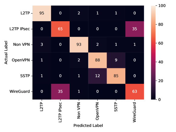
We can see that the classes that are misclassified are the classes for which the boundaries selected by HO Sizes provide the necessary separation. An optimized representation employing an $LR$ classifier with the same number of bins achieved an accuracy of $98\%$, in contrast to all other binning methods achieving accuracy lower than $90\%$, as the Uniform and Feature Selection approaches are limited to bins of equal size, and the bins selected by the Statistical approach were correlated to the overall data distribution but were unable to capture small nuances that affected the final classification performance.

7.2. Early Classification (EC) of Traffic

This section explores our EC setup, which is based on training multiple classifiers $f_{1},\ldots,f_{max}$ for multiple exit times $\tau_{1},\ldots,\tau_{max}$. When a classifier $f_{i}$ ($1\leq i<max$) achieves a confidence value larger than a threshold $\beta$, the classification stops and the label predicted by $f_{i}$ is reported. Otherwise, after the maximal exit time $\tau_{max}$, the label predicted by $f_{max}$ is reported (regardless of its confidence). A detailed explanation can be found in Section 5. In this section, for ease of presentation, we used a pseudo-logarithmic scale $(1ms,2ms,5ms,10ms\ldots)$.

First, to gain a sense of the behavior of the confidence for the different classifiers, we train the classifiers $f_{1},\ldots,f_{max}$ and checked their classification accuracy and coverage (the proportion of instances for which the classifier provides a prediction) for possible confidence thresholds.

The results for a single classification task (namely, VPN Services with 5 bins) are shown in Figure 8.

Figure 8. Graphs showing coverage and percentage of true and false predictions as a function of the confidence threshold, for classifiers of different exit times.

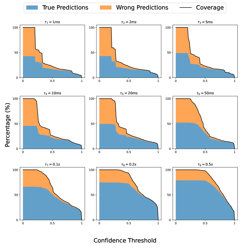
Some significant insights emerge from these results. First, even with short exit times, many samples have been classified with high confidence, thus validating the underlying principle of our method: many flows can be classified at an early stage, thereby reducing the average classification time and saving memory resources. Second, we observe an improvement in model coverage and accuracy over time, indicating that subsequent classifiers generally classify with higher accuracy and cover a broader range of flows. Yet, some flows are correctly classified in earlier classifiers but are misclassified in subsequent ones. This indicates that there are timely features that become hard to recognize after a longer period.

Following this experiment, we proceeded to evaluate the EC setup, where we determined the initial classification threshold $\beta$ based on the accuracy of a baseline model that classifies all flows after the maximal time $\tau_{max}$.

For the same classification task as shown in Figure 8 (VPN Services with 5 uniform bins), the EC model results are shown in Figure 9.

Figure 9. The percentage of flows classified up to each period (the coverage) in the EC setup. We can also see the amount of flows classified correctly and incorrectly. The final EC model’s accuracy is marked in red, while the predetermined threshold $\beta$ is marked in green.

(a) Average Exit Time

(b) Accuracy

Figure 10. The accuracy and the average exit time of EC models with different numbers of bins, across all classification tasks. Results are relative to the maximal time period $\tau_{max}$ and the corresponding classifier $f_{max}$ of each specific classification task and number of bins.

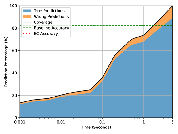
We can see two phenomena. First, the average classification time for flows stands at $1.01$ seconds, in contrast to the baseline model’s classification time of $5$ seconds, representing a notable improvement of approximately $80\%$ in classification speed.

Moreover, the final accuracy of the EC model surpasses that of the baseline model. This means that not only we can save classification time, but EC can potentially improve the model’s accuracy. As previously discussed, this improvement could stem from timely features identified by earlier models, which may go unnoticed by subsequent ones.

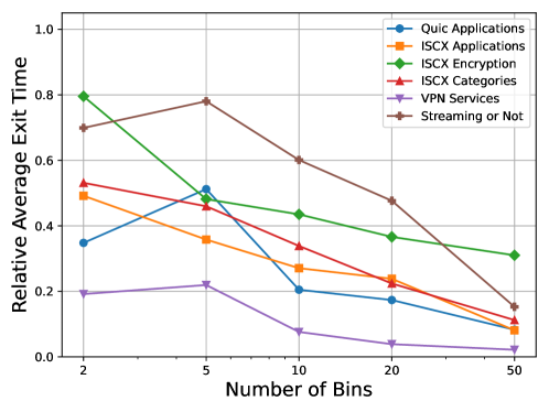
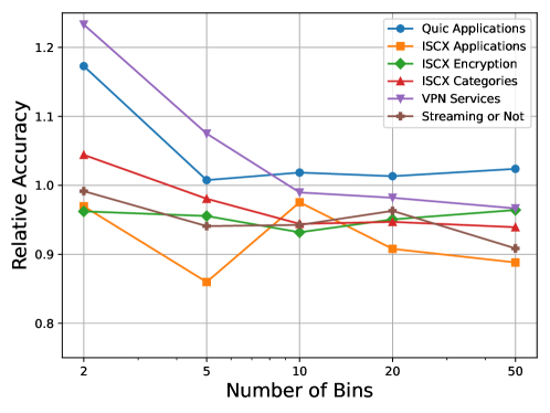
Figure 10 compares models utilizing EC for different tasks, where each value is normalized against a uniform binning model with the appropriate number of bins. These figures highlight the inherent trade-offs in employing $EC$: While larger representations facilitate faster classification, there is a slight compromise in accuracy compared to baseline models. On the other hand, smaller representations have the potential to surpass the performance of baseline models, as explained above.

The rationale behind these results lies in the fact that larger representations encapsulate finer details about the flows, thereby boosting the confidence of earlier models. Nevertheless, the notable enhancement in reducing classification time comes with the potential of misclassification at these early stages.

We also compare the results of the EC setup with a lower classification threshold ($\beta-\alpha$). The results of this comparison for one classification task are shown in Figure 11.

Figure 11. The accuracies and the average exit times of EC models with different thresholds, for the VPN Services classification task with 5 bins. $\beta$ is set to be the accuracy of the baseline model, and the threshold for each model is $\beta-\alpha$. Notice that the graph’s x-axis is not linear and shows the baseline model that classifies all flows after $\tau_{max}=5s$.

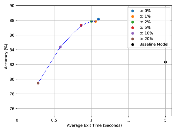
By opting for a lower threshold, a greater number of flows undergo early-stage classification, thereby reducing the average classification time. However, while the classification time is reduced, there is a notable decrease in accuracy. This tradeoff is controlled by selecting the threshold parameter, giving the flexibility to fine-tune this threshold according to specific requirements and constraints. In this experiment, it is evident that up to an $\alpha$ value of $5\%$, the decline in accuracy is negligible (lower than $1\%$), while there is a reduction of $25\%$ in collection time.

(a) VPN Services - 5 bins

(b) VPN Services - 10 bins

(c) VPN Services - 20 bins

(d) VPN Services - 50 bins

Figure 12. Accuracy as a function of the average classification time, created using different $\alpha$ values (as in Figure 11). Each graph compares the uniform and the logarithmic methods for creating the bins for the arrival-times dimension for a given number of bins.

7.3. Early Classification with Hyperparameter Optimization (ECHO)

Having noted the effectiveness of HO in enhancing model accuracy (Section 7.1), we aim to extend these representations to EC setups as well.

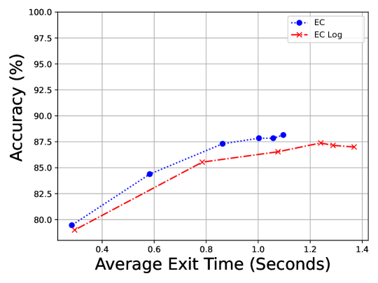
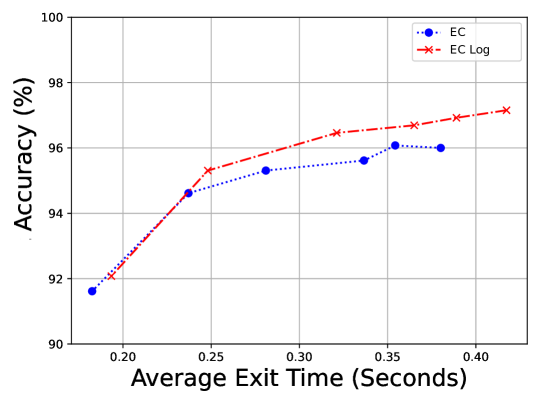
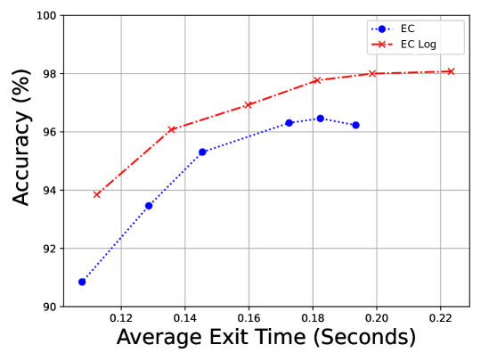
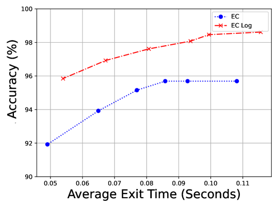
First, we will compare two methods for the bins of the arrival times distribution, the simple EC with uniform time and size bins, and the EC Log method with logarithmic time bins. The full description of those methods and how they are updated to allow real-time classification without memory overhead is in Section 6.

The comparison results for different numbers of bins and different $\alpha$ values are shown in Figure 12. The results for the two methods are similar. Yet, a noteworthy trend is that with smaller representations, the performance of EC Log is inferior. Conversely, for larger representations, EC Log tends to exhibit higher accuracy, surpassing the accuracy of the uniform EC. We observe that while introducing non-uniformity in the time dimension enhances accuracy, its impact is relatively minor compared to the non-uniformity seen in the packet-sizes dimension, as depicted earlier in Figure 5.

In the following experiment, we evaluate the creation of EC models with non-uniform bins in the packet size dimension, namely ECHO. As explained in Section 6, this process does not require any additional memory or computational power. For the ECHO models in this comparison, $\beta$ is selected as the accuracy of a baseline uniform model, and $\alpha$ is $5\%$ based on previous observations (Figures 11 and 12). The selected $\alpha$ value strikes a balance between average exit time and accuracy, with similar trends noted for other values of $\alpha$.

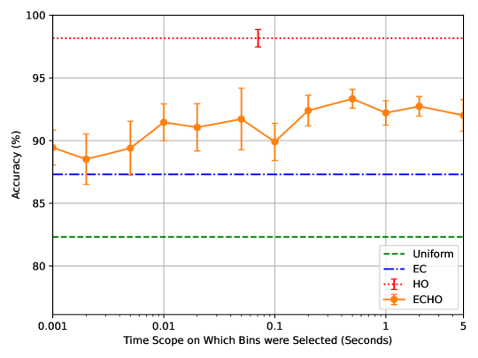
Figure 13 compares different selections of bins for the EC model, where each selection is based on an HO optimization over a classifier with the corresponding time scope $f_{1},\ldots,f_{max}$. Figure 13a compares the accuracy of the ECHO setups, it is noticable that ECHO significantly improves the model’s accuracy compared to the uniform EC model. However, the accuracy results are still lower than an HO setup (with non-uniform packet size bins) that classifies all flows after $\tau_{max}$.

Moreover, even though no specific classifier has a clear advantage in average accuracy, there is a smaller standard deviation for subsequent classifiers, implying that the binnings of these classifiers are more reliable and consistent, and therefore, are preferable.

(a) Accuracy

(b) Average exit time

Figure 13. Different bin selection methods for creating ECHO models. Uniform and HO models classify all flows after 5 seconds, while the EC and ECHO models perform early classification. ECHO models have optimized packet size bins based on different exit times. The error bars in the Bayesian results show the standard deviation of the results of the NCV process (see Section 4). Notice that the time-graph’s y-axis is not linear and shows the baseline models (Uniform or ECHO), classifying all flows after $\tau_{max}=5$.

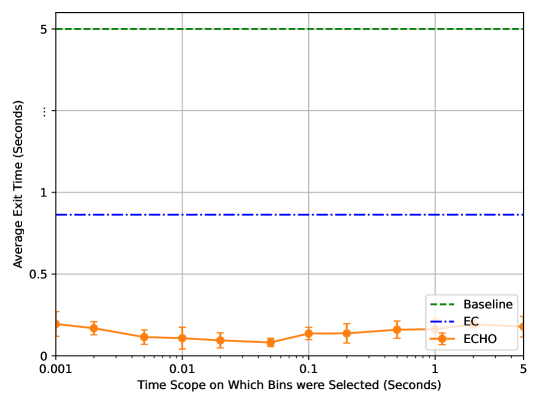
In Figure 13b, we compare the same classifiers in terms of average exit time. Here, for all binnings, the ECHO models show significantly faster average classification times (with no advantage to any specific selection). Recall that the threshold value for the EC models is based on a baseline uniform model, and as shown earlier, HO significantly improves accuracy, which is then reflected as well in higher confidence in classification. Thus enabling faster classification but with a lower accuracy than a full HO model.

8. Conclusions

This paper highlights the fact that many traffic classification techniques have considerable room for improvement. The techniques applied in the ECHO approach can seamlessly be combined with many existing traffic classification methods, and reduce both their memory footprint and their collection time without compromising any aspect of the classification process.

We show that by employing hyperparameter optimization methods to create non-uniform flow representations, we can significantly reduce the memory overhead of representations without compromising model accuracy. Furthermore, it boosts the model’s throughput as smaller and more efficient classifiers are used.

We also demonstrate that building a setup that includes multiple exit times with multiple classifiers, can significantly reduce the average required time for classification with no additional memory requirements.

In this paper, we utilize the TPE algorithm to optimize the variable-sized bins. Although this process is conducted offline, in future work, we aim to investigate other methods with improved time efficiency. We also wish to explore whether other flow representations could be optimized in terms of memory usage.

In addition, we aim to delve into different methods to create the setup for early traffic classification, and different methods for assessing the models’ confidence as part of the early classification process.

8.1. Reproducability

Our code, as well as the processed datasets, will be publicly available to the community upon completion of the double-blind review process of our paper.

8.2. Acknowledgments

Part of this work has been supported by Israel Innovation Authority within the ENTM consortium.

Appendix A Datasets

This section provides an overview of the three publicly available datasets used for training and testing our models, and the different classification tasks for each dataset.

Quic traffic dataset (Rezaei and Liu, 2020).

The Quic traffic dataset was recorded at UC Davis and consists of the traffic of 5 Google services (Google Drive, YouTube, Google Docs, Google Search, and Google Music) under several operating systems (including different Windows and Ubuntu distributions). The flow counts are shown in Table 3.

For this dataset, we consider one classification task, which we call Quic Applications, of classifying flows to one of the different applications.

ISCX combined traffic dataset.

This dataset consists of 2 network captures produced by the University of New Brunswick (Draper-Gil et al., 2016; Lashkari et al., 2017). The captures were filtered to include only the traffic related to the actual label of the flow. Classes with an insufficient number of samples (e.g., chat) were discarded. The processed dataset consists of 4 traffic categories (VoIP, video, file transfer, and browsing) with different applications for each category.

Table 3. The number of flows per application in the Quic traffic dataset.

Application	Number of Flows
Google Search	1915
Google Drive	1636
Google Doc	1221
Youtube	1077
Google Music	592

For these categories, we have 3 encryption techniques: non-VPN, VPN (for all classes except browsing), and TOR. As proposed in the original papers, the dataset is sampled using a 15-second non-overlapping time window and every sample is issued as a different flow. Table 4 shows the number of flows for each category and each type of encryption, while Table 5 delves into specific applications within the video and VoIP categories.

Table 4. The number of flows per category and encryption technique in the ISCX combined traffic dataset.

Category	Non-VPN	VPN	Tor
Voip	4397	1543	1761
Video	1180	301	438
File Transfer	954	303	546
Browsing	757	-	448

Table 5. The number of flows per application in the ISCX traffic dataset (Non-VPN).

Category	Application	Number of flows
VoIP	Facebook	1997
	Hangout	2441
	Skype	1823
	Voipbuster	1032
Video	Vimeo	565
	YouTube	534
	Hangouts	227
	Skype	210
	Netflix	207
	Facebook	176

For this dataset, we consider three classification tasks: (i) ISCX Applications in which we classify the different applications in Table 5; (ii) ISCX Encryption, in which we classify the different encryption protocols (namely, VPN, Non-VPN, or TOR); and (iii) ISCX Categories, in which we obtain the category (namely, video, VoIP, file transfer, or browsing) for the flow.

VPN services dataset (Naas and Fesl, 2023).

This dataset consists of packet captures produced and processed by the University of South Bohemia. The processed dataset contains 5 traffic categories (email, video conferencing, SSH, streaming, and non-streaming) using different applications for the streaming and non-streaming categories (the specific applications are not available in the dataset). Traffic from all categories is recorded over VPN and non-VPN connections, and using 7 different VPN settings (L2TP, L2TP IPsec, OpenVPN, PPTP, SSTP, WireGuard, and non-VPN).

Since the dataset contains a low volume of email, video conferencing, and SSH traffic, we only use the streaming and non-streaming categories. We also exclude the traffic recorded over PPTP VPN as it contains significantly fewer samples than the other VPN services. The number of flows in each category for the filtered dataset is shown in Table 6.

Table 6. The number of flow by category and VPN service in the VPN service dataset (Naas and Fesl, 2023).

VPN Protocol	non-streaming	streaming
L2TP	1003	94
L2TP IPsec	1003	93
Non VPN	3277	440
OpenVPN	999	96
SSTP	986	97
WireGuard	1003	99

For this dataset, we consider two classification tasks. First, VPN Services, is the task of classifying the specific VPN in use. Secondly, Streaming or Not is the binary task of categorizing the flows of the dataset into streaming/non-streaming categories.

A.1. Preprocessing

We filter the samples using three parameters: minimal number of packets, minimal volume (in bytes), and minimal duration. For every dataset, we have selected these parameters with regard to similar experiments done in the literature and to our observations of the traffic patterns. The selected parameters for each dataset are shown in Table 7.

Table 7. Preprocessing parameters

	Timeout $\tau$	Min. Packets	Min. Vol.	Min. Dur.
QUIC	1s	10	0	0.5s
VPN	5s	100	10KB	3s
ISCX	15s	100	10KB	5s

Additionally, as some of our datasets are imbalanced, we have employed random undersampling (Batista et al., 2004) to balance the data. This balancing procedure was applied to both the training and test sets to ensure equal representation of each class.

Appendix B Representations and Models Comparison

In this section, we thoroughly compare different representations with various sizes (detailed below), employing 4 different classifiers, Random Forest (RF) (Ho, 1995), Logistic Regression (LR) (Pearl and Reed, 1920), Support Vector Machine (SVM) (Cortes and Vapnik, 1995), and Convolutional Neural Networks (CNNs, denoted here by DEEP) (Fukushima, 1980). Although ECHO can work with any distributional representation and classifier, this comparison justify our selection of representation and model in Section 7.

Recall that we denote the selected representation type as $r$, where $r_{q}$ is the calculated representation for the flow with identifier $q$. We compare the following four common types of flow representations.

Distribution vectors,:

denoted by $dist(N)$. This representation consists of 4 distribution vectors of size $N$, containing, for each flow direction, counters of the arrival times and packet sizes, where each value is mapped to one of the $N$ bins, as suggested by (Engelberg and Wool, 2021). $dist(N)$ works under the classifiers $DEEP$ 1D-CNN, $RF$, $LR$, and $SVM$. The size of $dist(N)$ is $4N$ bytes as we store 4 vectors of size $N$, using 8-bit integers.

Time series,:

denoted by $ts(N)$. Time series of arrival time, packet size, and packet direction of $N$ packets, as proposed by (Bernaille et al., 2006a; Yang et al., 2021). $ts(N)$ works under the classifiers $DEEP$ 1D-CNN, $RF$, $LR$, and $SVM$. The size of $ts(N)$ is approximately $6N$ bytes as we store the arrival time (a 32-bit float), packet size (11 bits for sizes up to 1500), and direction (a boolean value) of $N$ packets.

FlowPic,:

denoted by $fp(N\times N)$. The FlowPic representation is a two-dimensional distribution matrix of size $N\times N$ of arrival times and packet sizes, as proposed by (Horowicz et al., 2022; Shapira and Shavitt, 2019; Engelberg and Wool, 2021; Finamore et al., 2023). As in $dist(N)$, each packet size and arrival time is mapped to one of $N$ bins. Then, element ($i$,$j$) in the matrix holds the number of packets whose arrival times are mapped to (arrival time) bin $i$, and packet sizes are mapped to (packet size) bin $j$.

$fp(N\times N)$ can be used under the classifiers $DEEP$ 2D-CNN, $RF$, $LR$, and $SVM$. The size of $fp(N\times N)$ is $2\cdot N^{2}$ bytes as we store a two-dimensional vector of size $N$ for each traffic side, using 8-bit integers.

Statistical Features,:

denoted by $sts$. Statistical representation, containing 33 basic statistical features, as proposed by (Williams et al., 2006; Draper-Gil et al., 2016; Lashkari et al., 2017; Anderson and McGrew, 2017) and others. The features are the basic minimum, maximum, mean, median, and standard deviation of the packet sizes and packet relative arrival times, for all packets and each traffic direction independently, as well as the number of packets for each direction. This representation is only used with simpler ML classifiers: $RF$, $LR$, and $SVM$. The size of $sts$ is $132$ bytes if all statistics are stored as 32-bit float values (this can be reduced by setting specific types to each value).

B.1. Flow Representations

The results for the different classification tasks are shown in Tables 8–13. For brevity, we show only the accuracy and exclude the std results of the $k$-fold process. Additionally, we note that the neural network architecture of the $DEEP$ CNNs is not relevant for small $dist$ and $ts$ representations (as it includes pooling layers), as well as $sts$ representations (which have no temporal structure).

Table 8. QUIC Applications classification task.

	RF	SVM	LR	DEEP
dist(5)	94.9%	82.7%	93.6%	-
dist(10)	95.9%	82.3%	95.5%	-
dist(20)	95.9%	82.2%	95.7%	94.9%
dist(50)	95.7%	79.4%	94.4%	96.2%
ts(5)	94.6%	81.3%	81.2%	-
ts(10)	95.1%	80.5%	79.3%	-
ts(20)	95.3%	84.5%	79.7%	94.7%
ts(50)	95.8%	85.5%	83.8%	93.3%
fp(8)	93.0%	78.7%	95.5%	95.2%
fp(16)	91.8%	69.8%	94.7%	94.7%
fp(32)	90.0%	66.9%	92.5%	95.5%
sts()	95.0%	82.9%	90.0%	-

Table 9. ISCX Applications classification task.

	RF	SVM	LR	DEEP
dist(5)	80.9%	73.3%	76.4%	-
dist(10)	87.0%	79.9%	91.8%	-
dist(20)	87.3%	82.8%	93.4%	95.9%
dist(50)	88.8%	91.7%	95.6%	97.8%
ts(5)	67.0%	49.5%	39.1%	-
ts(10)	68.5%	56.2%	42.9%	-
ts(20)	69.6%	60.1%	42.8%	53.5%
ts(50)	73.7%	61.1%	42.3%	73.9%
fp(8)	80.4%	72.3%	77.0%	78.0%
fp(16)	81.4%	74.9%	82.6%	91.4%
fp(32)	83.0%	85.3%	84.2%	94.5%
sts()	92.8%	69.3%	92.9%	-

Table 10. ISCX Encryption classification task.

	RF	SVM	LR	DEEP
dist(5)	92.3%	83.6%	81.1%	-
dist(10)	92.7%	85.5%	84.1%	-
dist(20)	92.8%	88.6%	90.2%	94.6%
dist(50)	90.8%	93.3%	91.6%	96.2%
ts(5)	81.2%	68.3%	60.8%	-
ts(10)	81.9%	69.8%	59.0%	-
ts(20)	83.0%	69.8%	58.0%	82.9%
ts(50)	84.6%	69.8%	58.3%	84.5%
fp(8)	90.7%	81.2%	84.5%	85.5%
fp(16)	92.1%	83.3%	88.4%	93.2%
fp(32)	85.4%	81.4%	88.1%	92.7%
sts()	95.2%	78.4%	82.5%	-

Table 11. ISCX Categories classification task.

	RF	SVM	LR	DEEP
dist(5)	89.1%	88.5%	82.6%	-
dist(10)	90.6%	89.5%	89.4%	-
dist(20)	91.1%	90.6%	93.3%	93.2%
dist(50)	89.4%	92.0%	91.5%	94.7%
ts(5)	77.3%	62.4%	55.3%	-
ts(10)	77.9%	68.1%	61.5%	-
ts(20)	76.7%	72.8%	64.1%	78.3%
ts(50)	76.5%	75.5%	63.9%	82.7%
fp(8)	85.8%	89.0%	87.6%	92.2%
fp(16)	83.1%	89.7%	88.7%	93.6%
fp(32)	80.7%	88.2%	88.5%	94.7%
sts()	92.3%	82.6%	86.5%	-

Table 12. VPN Services classification task.

	RF	SVM	LR	DEEP
dist(5)	90.3%	86.5%	82.3%	-
dist(10)	97.8%	98.7%	97.1%	-
dist(20)	98.9%	98.6%	98.4%	98.9%
dist(50)	99.7%	98.6%	99.0%	99.2%
ts(5)	92.2%	58.3%	36.0%	-
ts(10)	91.6%	63.2%	49.0%	-
ts(20)	92.4%	73.5%	60.0%	91.6%
ts(50)	91.7%	74.4%	62.0%	90.2%
fp(8)	96.2%	93.2%	95.9%	97.7%
fp(16)	96.7%	97.5%	97.5%	99.2%
fp(32)	95.4%	97.3%	97.2%	99.5%
sts()	96.2%	85.7%	93.4%	-

Table 13. Streaming or Not classification task.

	RF	SVM	LR	DEEP
dist(5)	82.4%	75.2%	69.8%	-
dist(10)	84.1%	80.0%	79.1%	-
dist(20)	82.2%	79.5%	79.4%	82.1%
dist(50)	80.4%	77.8%	78.5%	79.9%
ts(5)	68.1%	62.1%	59.3%	-
ts(10)	69.4%	65.3%	64.3%	-
ts(20)	69.9%	65.1%	64.4%	63.5%
ts(50)	69.5%	62.6%	63.1%	65.1%
fp(8)	79.1%	76.9%	75.9%	80.7%
fp(16)	79.1%	77.1%	78.5%	82.6%
fp(32)	76.3%	74.5%	76.2%	84.2%
sts()	80.1%	64.9%	71.7%	-

We observe some common trends for most of the tasks and representations:

First, $dist$ representations achieve the highest accuracy for most classification tasks (with two anomalies favoring $fp$), with the $DEEP$ CNN classifier achieving the highest accuracy. It is apparent that the distributional features in $dist$ and $fp$ representations hold meaningful information for classification more than raw values as a time series or a collection of statistical values.

Moreover, larger representations tend to achieve higher accuracy, this is due to the granularity of the representations which allows identifying intrinsic behaviors unnoticeable in smaller or more coarse representations.

Finally, small $LR$ classifiers tend to achieve a very low accuracy compared to other classifiers. However, this gap is significantly narrowed for larger representations, where $LR$ classifiers with larger representations achieve nearly equivalent results to those achieved by stronger $DEEP$ classifiers.

B.2. Models’ Deployment Considerations

In this section, we discuss the real-time deployment consideration of our classifiers. Particularly, we examine the memory requirements and the throughput of different representations and classifiers. First, we compare the memory required for storing all flow representations until classification. This is factored by the flow rate in the network, the collection time $\tau$, and by the representation size. We note that the memory required for storing the parameters of most classifiers is negligible compared to the flow representations.

Table 14 shows an approximation of the total required memory for storing flow representations. We can see that some representations (like larger $dist$ and $fp$ representations) may be impractical for real-time use on edge devices in a large network.

Table 14. Memory requirements for representation types (for the ISCX classification tasks), with $\tau=15s$ and a flow rate of 1 million flows per second.

	Repr. Size (B)	Approx. Required Memory (B)
dist(5)	20	300.0M
dist(10)	40	600.0M
dist(20)	80	1.2G
dist(50)	200	3.0G
ts(5)	30	450.0M
ts(10)	60	900.0M
ts(20)	120	1.8G
ts(50)	300	4.5G
fp(8)	128	1.9G
fp(16)	512	7.7G
fp(32)	2048	30.7G
sts()	132	2.0G

The second objective we explore is the throughput of the models. That is, the number of flows processed by a classifier within a specified timeframe, measured based on given computational capabilities. Specifically, we measured the number of flows classified within a 60-second period, using batches of 1000 samples. This method allows classifiers to perform batch operations more efficiently than single-sample classification (e.g. matrix multiplications).

Table 15. Classification throughput (in flows per second, using batches of 1K representations) for the ISCX Applications classification task.

	RF	SVM	LR	DEEP
dist(5)	96.3K	15.4K	7.7M	-
dist(10)	95.7K	13.8K	1.7M	-
dist(20)	93.7K	11.6K	1.4M	9.2K
dist(50)	89.2K	10.1K	894.2K	8.7K
ts(5)	95.5K	9.5K	7.4M	-
ts(10)	94.2K	9.4K	1.8M	-
ts(20)	91.0K	8.2K	1.4M	9.2K
ts(50)	84.9K	6.1K	937.1K	8.8K
sts()	94.2K	10.9K	1.8M	-
fp(8)	91.8K	10.1K	1.4M	9.0K
fp(16)	73.5K	3.5K	551.9K	7.8K
fp(32)	53.3K	766.7	177.6K	6.1K

Table 15 shows the throughput of different classifiers for different representations. It only includes the throughput calculated on models trained on the ISCX APPS classification task, however, as the required computational power merely changes across datasets or classification tasks, we observed similar results for the other tasks. The absolute numbers strongly depend on the deployment setting which in our case was an otherwise unloaded machine with an Intel core i7 processor (@ 2.80GHz 1.69GHz) with 16GB RAM, using Python’s Keras for $DEEP$ CNNs (with tensorflow CPU backend) and SKlearn for $RF$, $LR$, and $SVM$ classifiers.

We can see that despite the high accuracy achieved by $DEEP$ CNN classifiers, the classification throughput may be impractical if deployed in a large ISP network with millions of new flows per second. On the other hand, we can see that as expected, $LR$ classifiers outperform other classifiers in terms of throughput by an order of magnitude.

References

- (1)
- Aceto et al. (2019) Giuseppe Aceto, Domenico Ciuonzo, Antonio Montieri, and Antonio Pescapè. 2019. MIMETIC: Mobile encrypted traffic classification using multimodal deep learning. Computer Networks 165 (2019), 106944.
- Aceto et al. (2010) Giuseppe Aceto, Alberto Dainotti, Walter de Donato, and Antonio Pescapé. 2010. PortLoad: Taking the Best of Two Worlds in Traffic Classification. 2010 INFOCOM IEEE Conference on Computer Communications Workshops (2010), 1–5.
- Akbari et al. (2021) Iman Akbari, Mohammad A. Salahuddin, Leni Ven, Noura Limam, Raouf Boutaba, Bertrand Mathieu, Stephanie Moteau, and Stephane Tuffin. 2021. A Look Behind the Curtain: Traffic Classification in an Increasingly Encrypted Web. Proc. ACM Meas. Anal. Comput. Syst. 5, 1, Article 04 (feb 2021), 26 pages.
- Anderson and McGrew (2017) Blake Anderson and David McGrew. 2017. Machine Learning for Encrypted Malware Traffic Classification: Accounting for Noisy Labels and Non-Stationarity. In KDD’17. 1723–1732. https://doi.org/10.1145/3097983.3098163
- Anonymous (2023) Anonymous. 2023. Private Communincation..
- Barradas et al. (2021) Diogo Barradas, Nuno Santos, Luís Rodrigues, Salvatore Signorello, Fernando M. V. Ramos, and André Madeira. 2021. FlowLens: Enabling Efficient Flow Classification for ML-based Network Security Applications. In NDSS’21.
- Batista et al. (2004) Gustavo E. A. P. A. Batista, Ronaldo C. Prati, and Maria Carolina Monard. 2004. A Study of the Behavior of Several Methods for Balancing Machine Learning Training Data. SIGKDD Explor. Newsl. 6, 1 (jun 2004), 20–29. https://doi.org/10.1145/1007730.1007735
- Bergstra et al. (2011) James Bergstra, Rémi Bardenet, Yoshua Bengio, and Balázs Kégl. 2011. Algorithms for Hyper-Parameter Optimization. In Advances in Neural Information Processing Systems, Vol. 24.
- Bergstra et al. (2013) James Bergstra, Daniel Yamins, and David Cox. 2013. Making a Science of Model Search: Hyperparameter Optimization in Hundreds of Dimensions for Vision Architectures. In ICML’13 (Proceedings of Machine Learning Research, Vol. 28). PMLR, 115–123.
- Bernaille et al. (2006a) Laurent Bernaille, Renata Teixeira, Ismael Akodkenou, Augustin Soule, and Kave Salamatian. 2006a. Traffic Classification on the Fly. SIGCOMM Comput. Commun. Rev. 36, 2 (apr 2006), 23–26.
- Bernaille et al. (2006b) Laurent Bernaille, Renata Teixeira, Ismael Akodkenou, Augustin Soule, and Kave Salamatian. 2006b. Traffic classification on the fly. SIGCOMM Comput. Commun. Rev. 36, 2 (apr 2006), 23–26. https://doi.org/10.1145/1129582.1129589
- Bernaille et al. (2006c) Laurent Bernaille, Renata Cruz Teixeira, and Kave Salamatian. 2006c. Early application identification. In Conference on Emerging Network Experiment and Technology. https://api.semanticscholar.org/CorpusID:496969
- Bronzino et al. (2021) Francesco Bronzino, Paul Schmitt, Sara Ayoubi, Hyojoon Kim, Renata Teixeira, and Nick Feamster. 2021. Traffic Refinery: Cost-Aware Data Representation for Machine Learning on Network Traffic. Proc. ACM Meas. Anal. Comput. Syst. 5, 3, Article 40 (dec 2021), 24 pages.
- Cawley and Talbot (2010) Gavin C. Cawley and Nicola L.C. Talbot. 2010. On Over-Fitting in Model Selection and Subsequent Selection Bias in Performance Evaluation. J. Mach. Learn. Res. 11 (aug 2010), 2079–2107.
- Cortes and Vapnik (1995) Corinna Cortes and Vladimir Naumovich Vapnik. 1995. Support-Vector Networks. Machine Learning 20 (1995), 273–297.
- Draper-Gil et al. (2016) Gerard Draper-Gil, Arash Habibi Lashkari, Mohammad Saiful Islam Mamun, and Ali A Ghorbani. 2016. Characterization of encrypted and VPN traffic using time-related features. In ICISSP. 407–414.
- Engelberg and Wool (2021) Aviv Engelberg and Avishai Wool. 2021. Classification of Encrypted IoT Traffic Despite Padding and Shaping. arXiv:2110.11188 [cs.CR] https://arxiv.org/abs/2110.11188
- Enghardt et al. (2020) Reese Enghardt, Tommy Pauly, Colin Perkins, Kyle Rose, and Christopher A. Wood. 2020. A Survey of the Interaction between Security Protocols and Transport Services. RFC 8922.
- Ertam and Avcı (2017) Fatih Ertam and Engin Avcı. 2017. A new approach for internet traffic classification: GA-WK-ELM. Measurement 95 (2017), 135–142. https://doi.org/10.1016/j.measurement.2016.10.001
- Fahad et al. (2013) Adil Fahad, Zahir Tari, Ibrahim Khalil, Ibrahim Habib, and Hussein Alnuweiri. 2013. Toward an efficient and scalable feature selection approach for internet traffic classification. Computer Networks 57, 9 (2013), 2040–2057. https://doi.org/10.1016/j.comnet.2013.04.005
- Finamore et al. (2023) Alessandro Finamore, Chao Wang, Jonatan Krolikowski, José Manuel Navarro, Fuxing Chen, and Dario Rossi. 2023. Replication: Contrastive Learning and Data Augmentation in Traffic Classification Using a Flowpic Input Representation. Proceedings of the 2023 ACM on Internet Measurement Conference (2023). https://api.semanticscholar.org/CorpusID:262046478
- Finsterbusch et al. (2014) Michael Finsterbusch, Chris Richter, Eduardo Rocha, Jean-Alexander Muller, and Klaus Hanssgen. 2014. A Survey of Payload-Based Traffic Classification Approaches. IEEE Communications Surveys & Tutorials 16, 2 (2014), 1135–1156. https://doi.org/10.1109/SURV.2013.100613.00161
- Fukushima (1980) Kunihiko Fukushima. 1980. Neocognitron: A self-organizing neural network model for a mechanism of pattern recognition unaffected by shift in position. Biological Cybernetics 36 (1980), 193–202.
- Garcia and Korhonen (2018) Johan Garcia and Topi Korhonen. 2018. Efficient Distribution-Derived Features for High-Speed Encrypted Flow Classification. Proceedings of the 2018 Workshop on Network Meets AI & ML (2018). https://api.semanticscholar.org/CorpusID:51929029
- Haffner et al. (2005) Patrick Haffner, Subhabrata Sen, Oliver Spatscheck, and Dongmei Wang. 2005. ACAS: Automated Construction of Application Signatures. In ACM SIGCOMM MineNet’05. 197–202.
- Ho (1995) Tin Kam Ho. 1995. Random decision forests. In Proceedings of 3rd International Conference on Document Analysis and Recognition, Vol. 1. 278–282 vol.1. https://doi.org/10.1109/ICDAR.1995.598994
- Holland et al. (2021) Jordan Holland, Paul Schmitt, Nick Feamster, and Prateek Mittal. 2021. New Directions in Automated Traffic Analysis. In ACM CCS’21. 3366–3383.
- Horowicz et al. (2022) Eyal Horowicz, Tal Shapira, and Yuval Shavitt. 2022. A Few Shots Traffic Classification with Mini-FlowPic Augmentations. In ACM IMC’22 (Nice, France). 647–654. https://doi.org/10.1145/3517745.3561436
- Hughes (1968) Gordon P. Hughes. 1968. On the mean accuracy of statistical pattern recognizers. IEEE Trans. Inf. Theory 14 (1968), 55–63. https://api.semanticscholar.org/CorpusID:206729491
- Jacobs et al. (2022) Arthur S. Jacobs, Roman Beltiukov, Walter Willinger, Ronaldo A. Ferreira, Arpit Gupta, and Lisandro Z. Granville. 2022. AI/ML for Network Security: The Emperor Has No Clothes. In Proceedings of the 2022 ACM SIGSAC Conference on Computer and Communications Security (Los Angeles, CA, USA) (CCS ’22). Association for Computing Machinery, New York, NY, USA, 1537–1551. https://doi.org/10.1145/3548606.3560609
- Kohavi (1995) Ron Kohavi. 1995. A Study of Cross-Validation and Bootstrap for Accuracy Estimation and Model Selection. In International Joint Conference on Artificial Intelligence.
- Lashkari et al. (2017) Arash Habibi Lashkari, Gerard Draper-Gil, Mohammad Saiful Islam Mamun, and Ali A. Ghorbani. 2017. Characterization of Tor Traffic using Time based Features. In ICISSP.
- LEI (2014) JING LEI. 2014. Classification with confidence. Biometrika 101, 4 (2014), 755–769. http://www.jstor.org/stable/43304686
- Li et al. (2018) Rui Li, Xi Xiao, Shiguang Ni, Haitao Zheng, and Shutao Xia. 2018. Byte Segment Neural Network for Network Traffic Classification. 2018 IEEE/ACM 26th International Symposium on Quality of Service (IWQoS) (2018), 1–10. https://api.semanticscholar.org/CorpusID:59232416
- Lin (1991) Jianhua Lin. 1991. Divergence measures based on the Shannon entropy. IEEE Trans. Inf. Theory 37 (1991), 145–151. https://api.semanticscholar.org/CorpusID:12121632
- Liu et al. (2019) Chang Liu, Longtao He, Gang Xiong, Zigang Cao, and Zhen Li. 2019. FS-Net: A Flow Sequence Network For Encrypted Traffic Classification. IEEE INFOCOM 2019 - IEEE Conference on Computer Communications (2019), 1171–1179. https://api.semanticscholar.org/CorpusID:86515190
- Lopez-Martin et al. (2017) Manuel Lopez-Martin, Belen Carro, Antonio Sanchez-Esguevillas, and Jaime Lloret. 2017. Network Traffic Classifier With Convolutional and Recurrent Neural Networks for Internet of Things. IEEE Access 5 (2017), 18042–18050. https://doi.org/10.1109/ACCESS.2017.2747560
- Lotfollahi et al. (2017) Mohammad Lotfollahi, Mahdi Jafari Siavoshani, Ramin Shirali Hossein Zade, and Mohammdsadegh Saberian. 2017. Deep packet: a novel approach for encrypted traffic classification using deep learning. Soft Computing 24 (2017), 1999 – 2012. https://api.semanticscholar.org/CorpusID:35187639
- Moore and Papagiannaki (2005) Andrew W. Moore and Konstantina Papagiannaki. 2005. Toward the Accurate Identification of Network Applications. In PAM’05. 41–54.
- Moore and Zuev (2005) Andrew W. Moore and Denis Zuev. 2005. Internet Traffic Classification Using Bayesian Analysis Techniques. SIGMETRICS Perform. Eval. Rev. 33, 1 (jun 2005), 50–60.
- Naas and Fesl (2023) Mohamed Naas and Jan Fesl. 2023. A novel dataset for encrypted virtual private network traffic analysis. Data in Brief 47 (2023), 108945.
- Nguyen and Armitage (2008) Thuy T.T. Nguyen and Grenville Armitage. 2008. A survey of techniques for internet traffic classification using machine learning. IEEE Communications Surveys & Tutorials 10, 4 (2008), 56–76. https://doi.org/10.1109/SURV.2008.080406
- Pearl and Reed (1920) Raymond Pearl and Lowell J. Reed. 1920. On the Rate of Growth of the Population of the United States since 1790 and Its Mathematical Representation1. Proceedings of the National Academy of Sciences 6, 6 (1920), 275–288. https://doi.org/10.1073/pnas.6.6.275
- Rezaei and Liu (2020) Shahbaz Rezaei and Xin Liu. 2020. How to Achieve High Classification Accuracy with Just a Few Labels: A Semi-supervised Approach Using Sampled Packets. arXiv:1812.09761 [cs.NI] https://arxiv.org/abs/1812.09761
- Roughan et al. (2004) Matthew Roughan, Subhabrata Sen, Oliver Spatscheck, and Nick G. Duffield. 2004. Class-of-service mapping for QoS: a statistical signature-based approach to IP traffic classification. In ACM/SIGCOMM Internet Measurement Conference.
- Salman et al. (2020) Ola Salman, Imad H Elhajj, Ayman Kayssi, and Ali Chehab. 2020. A review on machine learning–based approaches for Internet traffic classification. Annals of Telecommunications 75, 11 (2020), 673–710.
- Shafiq et al. (2018) Muhammad Shafiq, Xiangzhan Yu, Ali Kashif Bashir, Hassan Nazeer Chaudhry, and Dawei Wang. 2018. A machine learning approach for feature selection traffic classification using security analysis. The Journal of Supercomputing 74 (2018), 4867–4892.
- Shapira and Shavitt (2019) Tal Shapira and Yuval Shavitt. 2019. Flowpic: Encrypted internet traffic classification is as easy as image recognition. In IEEE Infocom Workshops. 680–687.
- Sharafaldin et al. (2018) Iman Sharafaldin, Arash Habibi Lashkari, and Ali A. Ghorbani. 2018. Toward Generating a New Intrusion Detection Dataset and Intrusion Traffic Characterization. In ICISSP.
- Sivanathan et al. (2019) Arunan Sivanathan, Hassan Habibi Gharakheili, Franco Loi, Adam Radford, Chamith Wijenayake, Arun Vishwanath, and Vijay Sivaraman. 2019. Classifying IoT Devices in Smart Environments Using Network Traffic Characteristics. IEEE Transactions on Mobile Computing 18 (2019), 1745–1759. https://api.semanticscholar.org/CorpusID:70082542
- van Ede et al. (2020) Thijs van Ede, Riccardo Bortolameotti, Andrea Continella, Jingjing Ren, Daniel J. Dubois, Martina Lindorfer, David R. Choffnes, Maarten van Steen, and Andreas Peter. 2020. FlowPrint: Semi-Supervised Mobile-App Fingerprinting on Encrypted Network Traffic. Proceedings 2020 Network and Distributed System Security Symposium (2020). https://api.semanticscholar.org/CorpusID:211265114
- Wang et al. (2018) Wei Wang, Yiqiang Sheng, Jinlin Wang, Xuewen Zeng, Xiaozhou Ye, Yongzhong Huang, and Ming Zhu. 2018. HAST-IDS: Learning Hierarchical Spatial-Temporal Features Using Deep Neural Networks to Improve Intrusion Detection. IEEE Access 6 (2018), 1792–1806. https://doi.org/10.1109/ACCESS.2017.2780250
- Wang et al. (2017a) Wei Wang, Ming Zhu, Jinlin Wang, Xuewen Zeng, and Zhongzhen Yang. 2017a. End-to-end encrypted traffic classification with one-dimensional convolution neural networks. In 2017 IEEE International Conference on Intelligence and Security Informatics (ISI). 43–48. https://doi.org/10.1109/ISI.2017.8004872
- Wang et al. (2017b) Wei Wang, Ming Zhu, Jinlin Wang, Xuewen Zeng, and Zhongzhen Yang. 2017b. End-to-end encrypted traffic classification with one-dimensional convolution neural networks. 2017 IEEE International Conference on Intelligence and Security Informatics (ISI) (2017), 43–48. https://api.semanticscholar.org/CorpusID:3720713
- Wang et al. (2023) Yipeng Wang, Huijie He, Yingxu Lai, and Alex X. Liu. 2023. A Two-Phase Approach to Fast and Accurate Classification of Encrypted Traffic. IEEE/ACM Transactions on Networking 31, 3 (2023), 1071–1086. https://doi.org/10.1109/TNET.2022.3209979
- Williams et al. (2006) Nigel Williams, Sebastian Zander, and Grenville Armitage. 2006. A preliminary performance comparison of five machine learning algorithms for practical IP traffic flow classification. SIGCOMM Comput. Commun. Rev. 36 (10 2006), 5–16. https://doi.org/10.1145/1163593.1163596
- Xu et al. (2023) Yuwei Xu, Jie Cao, Kehui Song, Qiao Xiang, and Guang Cheng. 2023. FastTraffic: A lightweight method for encrypted traffic fast classification. Computer Networks 235 (2023), 109965. https://doi.org/10.1016/j.comnet.2023.109965
- Yang et al. (2021) Lixuan Yang, Alessandro Finamore, Feng Jun, and Dario Rossi. 2021. Deep Learning and Zero-Day Traffic Classification: Lessons Learned From a Commercial-Grade Dataset. IEEE TNSM 18, 4 (2021), 4103–4118. https://doi.org/10.1109/TNSM.2021.3122940
- Zhao et al. (2021) Jingjing Zhao, Xuyang Jing, and Witold Pedrycz. 2021. Network traffic classification for data fusion: A survey. Information Fusion 72 (02 2021). https://doi.org/10.1016/j.inffus.2021.02.009
- Zou et al. (2018) Zhuang Zou, Jingguo Ge, Hongbo Zheng, Yulei Wu, Chunjing Han, and Zhongjiang Yao. 2018. Encrypted Traffic Classification with a Convolutional Long Short-Term Memory Neural Network. 2018 IEEE 20th International Conference on High Performance Computing and Communications; IEEE 16th International Conference on Smart City; IEEE 4th International Conference on Data Science and Systems (HPCC/SmartCity/DSS) (2018), 329–334. https://api.semanticscholar.org/CorpusID:59233070