On a conjecture of a Pólya functional for triangles and rectangles
Abstract.
We consider the functional given by the product of the first Dirichlet eigenvalue and the torsional rigidity of planar domains normalized by the area. This scale invariant functional was studied by Pólya and Szegő in 1951 who showed that it is bounded above by 1 for all domains. It has been conjectured that within the class of bounded convex planar domains the functional is bounded below by and above by and that these bounds are sharp. Remarkably, the conjecture remains open even within the class of triangles. The purpose of this paper is to prove the conjecture in this case. The conjecture is also proved for rectangles where a stronger monotonicity property is verified. Finally, the upper bound also holds for tangential quadrilateral.
Key words and phrases:
torsion function, torsional rigidity, Dirichlet Laplacian, Dirichlet eigenvalue, sharp inequality1991 Mathematics Subject Classification:
Primary 35P15 , 49R05 ; Secondary 49J40, 35J251. Introduction and Main Results
Consider an open connected set , , which we refer to as a domain. Further, assume the Lebesgue measure of , denoted by , is finite. The torsion function is the unique weak solution to the boundary value problem
| (1.1) |
It is well known that , and . In fact, satisfies the isoperimetric inequality , where , is the ball centered at the origin with . It is also a well-known (and widely-used) fact that , where the right hand side is the expectation of the first exit time of Brownian motion from the domain starting at the point . Although this probabilisitic interpretation is very useful in many ways, it will not be explicitly used in this paper other than from time to time to observe domain monotonicity of various quantities.
The torsional rigidity of is defined by
The torsional rigidity has been studied and applied extensively in the theory of elasticity [Timoshenko-Goodier]. The torsional rigidity is related to the computation that measures the resistance of a beam with cross-sections to twisting forces. Probabilistically, the quantity can be written as which is the mean exit time of Brownian motion started in whose starting point is averaged by the uniform distribution on .
Let be the first Dirichlet eigenvalue of . In [Polya-1948b], Pólya showed that the process of Steiner symmetrization decreases while increasing . In this paper, we study the relation between and through the following functional
| (1.2) |
which we refer to by the Pólya functional following [Vandenberg-Ferone-Nitsch-Trombetti-2019a]. This functional was studied by Pólya-Szegő [Polya-Szego-1951, p. 91] in 1951 who showed that . This was known to Pólya as early as 1947 in [Polya-1947a, Eq. (2)]. By a result in [Vandenberg-Ferrone-Nitsch-Trombetti-2016, Theorem 1.2], this bound is sharp over all open connected sets in . The problem of obtaining sharp upper and lower bounds on this functional and its extremals for subclasses of domains has been extensively investigated for many years, and especially in the last ten years or so. Among the class of bounded convex domains in the plane the following conjecture is open.
Conjecture 1.1 (Conjecture 4.2 in [Berg-Buttazzo-Pratelli-2021], see also [Berg-Buttazzo-Velichkov-2015, Vandenberg-Ferrone-Nitsch-Trombetti-2016]).
For all bounded convex planar domains ,
| (1.3) |
and these bounds are sharp. The lower bound is attained for a collapsing sequence of isosceles triangles converging down to an interval. The upper bound is attained by a sequence of elongating rectangles approaching the infinite strip.
Remarkably, the conjecture remains open even within the class of triangles. The purpose of this paper is to prove the conjecture in this case. We will also consider a tangential quadrilateral, which is any convex quadrilateral that contains an incircle that is tangent to all sides. Examples include kites which include rhombi.
Theorem 1.2.
Suppose is a triangle or a rectangle. Then
| (1.4) |
The upper bound is attained for a sequence of elongating rectangles approaching an infinite strip. The lower bound is attained for any sequence of triangles collapsing down to an interval.
The upper bound also holds for any tangential quadrilateral.
Remark 1.3.
A stronger monotonicity result is given for rectangles, where in Theorem 7.1 it is shown that is increasing for for rectangles .
As already mentioned, while Conjecture 1.1 remains open for general convex domains, progress has been made for other smaller classes of domains. In [Vandenberg-Ferone-Nitsch-Trombetti-2019a], the authors proved that the lower bound of Conjecture 1.1 is true for all domains that are either isosceles triangles or rhombi. Moreover, they show this inequality is sharp for a limiting sequence of collapsing isosceles triangles or rhombi that converge to an interval. It has also been shown in [Berg-Buttazzo-Pratelli-2021, Proposition 5.2] or [Briani-Buttazzo-Prinari-2022, Theorem 4.4] that the asymptotic limit of for thinning sequences of convex domains are always between the conjectured bounds.
In this paper we shall only be concerned with domains in the class of planar bounded convex domains. Some improvements on the upper bound valid for all planar domains have been obtained for the class . For example, the bound was given in [Vandenberg-Ferrone-Nitsch-Trombetti-2016]. The best bound to date for all is given in [Ftouhi-2022]. Recently in [Berg-Bucur-2024], it has been shown that there exists a such that for all simply connected planar domains. Improved lower bounds for for all have also been obtained. In particular, it was shown in [Vandenberg-Ferrone-Nitsch-Trombetti-2016] that on . This has been improved to for planar convex domains in (see [Briani-Buttazzo-Prinari-2022, Prop. 3.2] and [Brasco-Mazzoleni-2020, Remark 4.1]).
In general, other than a few special cases, there are no explicit formulas for the torsional rigidity or the first Dirichlet eigenvalue of triangles or general polygons. This makes proving sharp inequalities involving both and difficult even for triangles. Despite this, sharp inequalities for the first Dirichlet eigenvalue of triangles, quadrilaterals and other polygons have been extensively investigated in the literature. We point to the works of [Freitas-2007, Freitas-2006, Antunes-Freitas-2006, Freitas-Laugesen-2021, Antunes-Freitas-2011, Endo-Liu-2023, Solynin-Zalgaller-2010, Arbon-etall-2022, Arbon-2022, Laugesen-etall-2017, Siudeja-2016, Indrei-2024] for some of this literature. In particular, the inequalities and methods from [Freitas-Siudeja-2010, Siudeja-2007, Laugesen-Siudeja-2011, Siudeja-IU-2010] will be useful in the proof of our main result for various cases. Although not as extensive, there is also a sizable literature regarding the torsional rigidity of polygons; see [Rolling-2023, Solynin-2020, Fleeman-Simanek-2019, Solynin-Zalgaller-2010, Benson-Laugesen-Minion-Siudeja-2016, Timoshenko-Goodier]. Although not directly related, it is interesting to note that other difficult spectral theory problems have also been studied for triangles. One such example is the well known Hot Spots Conjecture regarding the maximum of the Neumann eigenfunction corresponding to the first positive eigenvalue that was settled recently in [Judge-Sugata-2019] for triangles, with earlier and recent contributions given by several authors [Siudeja-HotSpots-2015, Chen-Changfeng-Ruofei-2023, Banuelos-Burdzy-1999]; see also the Polymath Project 7 [Polymath]. That conjecture remains open for general convex domains. Inverse spectral problems have also been considered for triangles such as in [Gomez-Serrano-Orriols-2021, Meyerson-McDonald-2017] and higher -moment spectrum bounds have been studied in [Dryden-Langford-McDonald-2017].
We now discuss other functionals where their sharp bounds would imply sharp bounds for . Consider the functional given by
where is the inradius. By the results in [Brasco-Mazzoleni-2020, Polya-Szego-1951] it follows that for . Combining this with the Hersch-Protter inequality gives the best known bound of , as mentioned in [Brasco-Mazzoleni-2020, Remark 4.1].
There is another functional whose lower bounds imply lower bounds for . The mean-to-max ratio of the torsion function (also referred to as the “efficiency") is defined by
where is the maximum of the torsion function . Various authors have proved upper and lower bounds for over convex domains for more general operators; see [DellaPietra-Gavitone-Guarino-2018, Bueno-Ercole-2011, Henrot-Lucardesi-Philippin-2018, Briani-Bucur-2023]. The best lower bound so far is given in [DellaPietra-Gavitone-Guarino-2018]. A result by Payne in [Payne-1981] shows that . Combining these two bounds implies that . It is conjectured in [Henrot-Lucardesi-Philippin-2018] that the bound holds for convex planar domains which would also imply the conjecture on .
1.1. Discussion of method of proof
As mentioned before, there are no explicit formulas for the first Dirichlet eigenvalue nor for the torsional rigidity of arbitrary triangles. Moreover, what makes the study of extremal domains difficult for the functionals mentioned above, including the Pólya functional studied in this paper, is the competing symmetries in the problem. While the classical symmetrizations techniques, such as spherical or Steiner symmetrization, increase the torsional rigidity, they decrease the eigenvalue. At present there are no general techniques (symmetrization or other types) that give the increasing, or decreasing, of the product as a single unit. Thus, the results are obtained by developing ad-hoc techniques. For example, for the lower bound of the product one finds good lower bounds for each quantity involved and similarly for the upper bound of the products. This requires dividing domains into various geometric cases and applying different techniques to different cases.
In the case for triangles our approach is to split the proof into several acute and obtuse cases to prove the lower bound. We rely on various different techniques to obtain the required bounds depending on the cases. We use domain monotonicity to compare with other domains where explicit formulas are known. We also use various inequalities for the first Dirichlet eigenvalue proved in [Freitas-Siudeja-2010, Siudeja-2007, Laugesen-Siudeja-2011, Siudeja-IU-2010]. We use the variational characterization of the torsional rigidity (see (2.2)) to prove new lower bounds for the torsional rigidity. In some of the cases, we rely on Steiner symmetrization to give a bound for the eigenvalue in terms of other triangles. The most difficult cases concerns those of the thin triangles where approaches the sharp lower bound . In these cases, given in Proposition 3.3 and 4.3, the new idea is to use a monotonicity result (Lemma 3.4 and 3.5) to reduce to a lower bound for right triangles.
All of the derived bounds are done analytically. Some of the inequalities are shown by proving various technical lemmas on explicit functions. Some of the lemmas are reduced to proving polynomial inequalities, of which we adopt a method of Siudeja given in [Siudeja-IU-2010, Section 5]. The upper bound will rely on previous known bounds by Siudeja, Makai and Solynin-Zalgaller. The monotonicity result for the Pólya functional for rectangles follows from an explicit infinite series expression obtained from the classical expansion of the Dirichlet heat kernel for rectangles in terms of the eigenvalues and eigenfunctions.
1.2. Organization of the paper
The paper is organized as follows. Section 2.1 gives the geometric description for arbitrary triangles in terms of the pair of parameters . In terms of these parameters, one can describe the cases of (1) obtuse, (2) acute, (3) isosceles and (4) right, triangles. See Figure 1. This section also recalls the exact formulas for the torsion function, torsional rigidity, eigenfunction, eigenvalue and Pólya functional for the equilateral triangle, one of the few triangles where all the quantities are known. Section 2.2 gives several Lemmas proving lower bounds on quantities that will be used in the various cases for the lower bound estimate in Theorem 1.2. Section 3 proves the lower bound for Theorem 1.2 for acute and right triangles. Section 4 proves the bound for obtuse triangles. The announced upper bounds are proved in Section 5, both for triangles and tangential quadrilaterals. Section 5 also contains Proposition 5.2 which shows the sharpness of the lower bound of Theorem 1.2 for any sequence of thinning triangles. Section 6 collects all the bounds to conclude the proof of Theorem 1.2 for triangles. Section 7 proves Theorem 1.2 in the case of rectangles and shows the monotonicity as stated in Remark 1.3.
2. Preliminaries for triangles
2.1. Proof set up
Consider a triangle with vertices on , , with sides of length and . By translation, rotation, and scaling invariance of , it is enough to consider triangles of the form whose admissible set of points come from
Note that . Let be the angle between the sides of length , so that by the law of cosines we have . Using this we can observe the following. Theobtuse triangles correspond to the case when which occurs exactly when ,. The right triangles correspond to the curve , . The acute triangles correspond to , , outside of the obtuse region. Finally, the isoscele triangles correspond to those on the part of the circle , , and also the vertical line for . See Figure 1. We will mainly use this characterization when dealing with triangles that are obtuse so that where
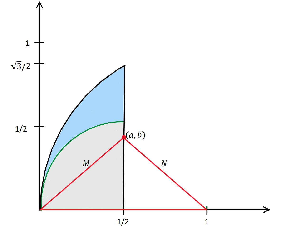
For acute and right triangles, we will use a different characterization of triangles. In particular, we can write any acute and right triangle as with side lengths such that . We will still associate this triangle with the one whose vertices are at , and but now take where
Throughout the paper, and no matter the characterization, we define to be the top angle between the sides of length . We define to be the bottom right angle between the sides of length and , while is the bottom left angle between the sides of length and . When using the characterization it turns out that is the length of largest side of and . Moreover, using we have that . When using the characterization it turns out that is the length of the smallest side of and . Moreover, using we have that . When convenient, we denote when we are dealing with the lengths of the sides of the triangle. Notice that .
We will use the different characterizations depending on the different cases that we shall consider and what is most convenient for our computations. The idea of the proof of Theorem 1.2 is to split the admissible sets into various regions and use different estimating techniques depending on the region. Often the regions will depend weather is far away from the equilateral triangle or not.
The equilateral triangle corresponds to with vertices at The torsion function for the equilateral triangle is given by
| (2.1) |
and a first Dirichlet eigenfunction for is given by
Moreover the following are well known
2.2. Preliminary Lower Estimates
We use various methods to estimate . One method of estimating will be through the following variational formula
| (2.2) |
We can find a test function for estimating by using a linear transformation of . In particular, a test function for any triangle is given by
| (2.3) |
Since the triangle is bounded by the lines then it is clear that on and . This test function is similar to the ones used in [Freitas-2006, Siudeja-2007, Laugesen-Siudeja-2011] to obtain upper estimates for but with replaced by the first eigenfunction .
We can then obtain the following estimate on with this test function. This bound will help when dealing with triangles that are closer to the equilateral triangle.
Lemma 2.1.
Using the test function in we obtain
for any .
Proof.
A computation shows that
∎
A circular sector of radius and angle turns out to be a good domain to estimate triangles. The following lower bound on sectors are good for triangles that are long and thin. The bound will be in terms of which denotes the th positive zero of the Bessel function . We denote its first zero. This lemma follows directly from [Siudeja-IU-2010, Theorem 1.3] and we state it here for easy reference of its explicit bound.
Lemma 2.2.
Let and be the angle of triangle between the edges of length and . Let be the sector with angle and radius such that . Then
Moreover, if and is the angle of triangle between the edges of length and then
Proof.
If then is the smallest angle. Let the sector such that . Since and , then so that . Now by [Siudeja-IU-2010, Theorem 1.3] it is shown that
where is the first zero of the Bessel function . If , then the angle is the smallest angle hence the rest of the proof is done similarly. ∎
Another method we will use throughout the paper will be the domain monotonicity properties of and . It is clear from the variational principal of both and that if then while . The domain monotonicity of also follows easily from the probabilistic definition of . This is clear since if then a Brownian path started in has to exit before exiting . Hence for , which implies .
The following bound will be useful when dealing with tall and long triangles.
Lemma 2.3 (Bound for Acute/Right triangle case).
Consider a triangle of side lengths where . Suppose (1) , or (2) holds. Then
where is the angle between the sides of length and is the altitude of the isosceles triangle of lengths with the same angle between the side lengths and . Note that satisfies
Proof.
Consider the circular sector
It is known that (see [Timoshenko-Goodier, pp. 278-280] and [Vandenberg-Ferone-Nitsch-Trombetti-2019a, Equation (5.6)])
and
Recall that denotes the angle between the sides of length and . Consider the isosceles triangle with angle and side lengths . It is clear that this triangle is inside . The shortest side of this isosceles triangle cannot have length greater than . Thus its altitude satisfies . See Figure 2.
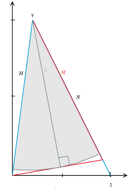
Hence the sector satisfies so that
Given , we know that since an isosceles triangles maximizes .
Case (1): An elementary computation shows that if
then
Hence, this is true whenever and .
Case (2): A similar elementary computation shows that
as long as . Hence this minimization problem is true for all .
In both cases we can use that fact that for all and all admissible , we have
which gives
Since
we can rewrite
which is the desired lower bound. ∎
We also need the following elementary geometric lemma which is proved here for completeness.
Lemma 2.4.
Consider a right triangle and let be the angle between the sides and . Let be the altitude of the isosceles triangle of lengths with the same angle between the side lengths and . Then
Proof.
First note that . Recall that is the altitude between the isosceles triangle of length and angle between the two side lengths . The law of cosines says that if is the angle between side lengths , and is the opposite side of then
First we find the angle of between side lengths , and note that . Let be the triangle of side length , (see Figure 3)
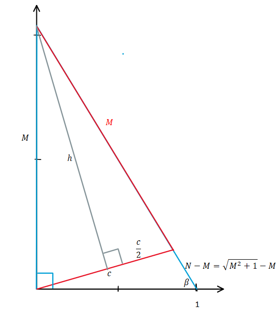
we can solve for ;
Hence,
Let be the right triangle inside of side lengths . Using the Pythagorean theorem we obtain
so that
Hence as desired. ∎
3. Proof of Theorem 1.2: Lower Bound for Acute and Right Triangles
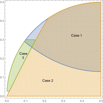
We will split the proof into two main cases. See Figure 4 for a picture of the regions for .
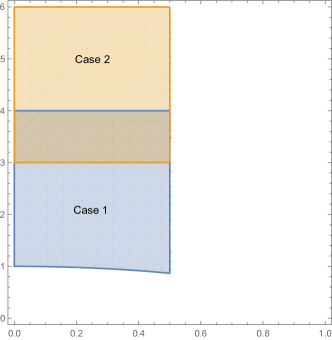
We first consider acute and right triangles that are close to the isosceles right triangle and equilateral triangle.
Proposition 3.1 (Case 1).
If then
Proof.
We split the rest of the proof into two cases with some overlap, of which there are some overlap.
Case 1a: Consider the region . Recall that this includes the equilateral triangle . By a result of Freitas and Siudeja in [Freitas-Siudeja-2010, Corollary 4.1] we have the following bound for the eigenvalue of a triangle,
where is the diameter and is the height perpendicular to its longest side. If then . Since , then so that
Putting this together with the bound
from Lemma 2.1, gives
Define
An elementary calculation shows that
which gives as needed.
Case 1b: We consider the region .
Here we estimate differently. First, using Steiner symmetrization with respect to the horizontal axis we have that since then
Let be the smallest angle between the sides of . Let be the circular sector such that . By Lemma 2.2 we have that
By Lemma 2.1 and using the fact that so that , we have
Putting these bounds together we obtain,
The zeros of Bessel function can be bound by given in [Qu-Wong-1999] where is the th negative zero of the Airy function . We then have that
Using the known fact that , it follows that
A simple computation leads to
Making the substitution by letting leads to and . Hence
Now note that
The following bounds can be obtained using a repeated application of
and the fact that :
Hence
This shows that for any and we have . To prove for this range, it suffices to prove that the function satisfies
which is done in the following Lemma. ∎
Lemma 3.2.
The function
satisfies , for .
Proof.
We prove the inequality for . Note that
then use so that it suffices to show
for . Rewriting this as a polynomial inequality, it suffices to show that
Expanding with we have
Then using , it suffices to show that the polynomial
| (3.1) |
satisfies , for . We now use the Siudeja algorithm described in Section 8 to show , as desired. This algorithm was introduced by Siudeja in [Siudeja-IU-2010] and it allows us to show any polynomial is negative on an interval given that the interval is small enough. Using the algorithm in Section 8.1 shows the desired inequality. ∎
In the following, we consider acute and right triangles that are long and thin. These triangles are far from the equilateral triangle and approach the degenerating lower bound of . We bound the torsional rigidity and principal eigenvalue using sectors with bounds given in Lemma 2.3 and Lemma 2.2. Afterwards, one of the key ideas will be to use monotonicity results given in Lemmas 3.4 and 3.5 to reduce to a lower bound for right triangles.
Proposition 3.3 (Case 2).
If then
Proof.
To estimate we will use Lemma 2.3. As in Lemma 2.3, let be the altitude between the isosceles triangle of length and angle between the two side lengths .
Since , by Lemma 2.3 we have that
where . Recall that by Lemma 2.2 we have and that
where . Thus
Putting these bounds together we have that
| (3.2) |
Note that given a fixed , we have that for any ,
Hence by Lemma 2.4
| (3.3) |
Using in we have that
| (3.4) |
Note that for a given and fixed , we have for any ,
This gives
| (3.5) |
Also recall that so that
Since are decreasing in , for all of , we have
Using in and the fact that the function
is increasing for Lemma 3.4 gives that
where
Lemma 3.4.
The function
where , is increasing in the interval .
Proof.
Making the substitution , it suffices to show
is increasing for .
We know that
where the remainder term satisfies , when is even and , when is odd and it converges on . Hence
where the remainder term when is odd which converges on . Hence
where and . Expanding out we have
where
and
| (3.6) |
The polynomial is certainly increasing for again applying Siudeja’s algorithm (see Section 8.2) to to show that . Moreover, the polynomial
has positive powers of with positive coefficients which means is increasing. This shows is increasing on the desired interval as needed. ∎
Lemma 3.5.
The function
where and satisfies for all .
Proof.
We make the substitution so that hence we define the function for by
Now since
we have
Using the elementary bounds , for so that for and
we have that
Thus,
It suffices to show for when , since . To do this we consider the polynomial
We want to show that this polynomial satisfies on . Making the substitution gives
| (3.7) |
We can show is negative on by applying Siudeja’s algorithm in Section 8.3. ∎
4. Proof of Theorem 1.2: Lower Bound for Obtuse and Right Triangles
Consider a triangle with vertices , , and with sides of length and . Recall that by the discussion in Section 2, to prove the desired bounds for all obtuse triangles we will use the following characterization
We will split the proof into three main cases. See Figure 5 for a picture of the regions for .
For two of the propositions below we will use the following bound by Freitas and Siudeja in [Freitas-Siudeja-2010, Corollary 4.1]
| (4.1) |
where is the diameter and is the height perpendicular to its longest side. If we have that and so that
| (4.2) |
Proposition 4.1 (Case 1).
If , then
for
when
Proof.
Proposition 4.2 (Case 2).
If , then
for .
Proof.
To bound the torsional rigidity we use the following test function (similar to the one used in [Vandenberg-Ferone-Nitsch-Trombetti-2019a, Section 5.1]) in the variational characterization of :
The triangle is bounded by when , by , when , and by , when . It is then clear that vanishes on the boundary. A straightforward computation shows that
Next, we prove the result for degenerating obtuse triangles that are close to right triangles. This will be the most difficult case in this section. The proof is similar to the proof of Proposition 3.3 in the acute case. We use sectors to give the appropriate lower bounds and then use the monotonicity results from Lemmas 3.4 and 3.5 to reduce to a lower bound for right triangles.
Proposition 4.3 (Case 3).
If , then
for and .
Proof.
We first give an estimate for the torsional rigidity. This estimate will be similar to the acute case given in Proposition 3.3.
Let and in particular consider
For obtuse triangles one can see that where is the side of middle length and is the smallest angle on the lower right. This containment can be checked using elementary geometry with a circle centered at of radius and noting that such a circle must be contained in since the angle between sides of length has an angle greater than . This implies that
Recall that . We first like to give a bound on the range of . Consider
where is the intersecting point for the curves and . Note that . For any fixed , one can see that is an increasing function of . For , one has that the angle is maximized when and so that in this region. Now recall that for we have
so that
Since
we can rewrite
Using Lemma 2.2 for the obtuse case we have that
and using the same estimates as in the proof of Proposition 3.1 we have that
with . This gives that
Recall that for any fixed the angle is an increasing function of . This means for any fixed , the angle is minimized by , which falls on the curve that represents the right triangles. By Lemma 3.4, the map
is increasing for , so that since we have
where . Using Lemma 3.5 shows that the factor
satisfies for . Noting that
whenever gives the desired bound for the factor .
Finally, we’d like to show the leftover factor term above is also greater than . To see this we simplify
and an elementary computation shows that this term is greater than for . Putting these bounds together shows the desired result for . ∎
5. Proof of Theorem 1.2: Upper Bound for triangles and tangential quadrilaterals
The upper bound for triangles and tangential quadrilaterals will follow by the following proposition. Rectangles that are not squares are not tangential quadrilaterals, hence it will be treated separately in Section 7.
Proposition 5.1.
For all triangles we have
| (5.1) |
Moreover, for any tangential quadrilateral we have
| (5.2) |
Proof.
Let denote the perimeter of a convex domain . By a result of Makai [Makai-1962] (see also a more general version given in [Fragala-Gazzola-Lamboley-2013]), we have that for all planar convex domains
| (5.3) |
where this upper bound is achieved by thinning isosceles triangles. Moreover, a result of Siudeja [Siudeja-2007] (see also [Solynin-Zalgaller-2010] for a different proof) gives that
| (5.4) |
where the upper bound is sharp for the equilateral triangle. Using and we have
as needed.
Moreover, for any tangential quadrilateral , we have
| (5.5) |
by a result of Solynin and Zalgaller in [Solynin-Zalgaller-2010, Corollary 3]. Combining (5.5) with Makai’s inequality it follows that
∎
We also give the following upper bound which gives the sharpness of the lower bound of Theorem 1.2 for thinning triangles and tangential polygons. Recall that denotes the inradius of the domain .
Proposition 5.2.
Suppose is a convex planar domain satisfying (such as triangles and tangential polygons). Then
Moreover, if is a sequence of such domains so that , then
Proof.
By [Ftouhi-2021, Corollary 1], we have the following bound for convex domains satisfying :
Using Makai’s inequality it follows that
as required. ∎
6. Proof of Theorem 1.2 for all triangles
Proof of Theorem 1.2.
We collect all the results to prove our main theorem on triangles. Recall that for the acute case/right triangle case we use the following representation,
while for the obtuse case we use the following representation
Part (a): Acute Lower bound: Let . The lower bound follows by Proposition 3.1 for and by Proposition 3.3 for .
Part (b): Obtuse Lower bound: Let . The lower bound follows by Proposition 4.1 for
when
The lower bound also follows by Proposition 4.2 for and by Proposition 4.3 for
All these regions combined make up (see Figure 5).
Part (c): Upper Bound: This follows by Proposition 5.1.
Part (d): Sharpness of the lower bound for triangles:
Let be a sequence of triangles collapsing down to an interval. Then by a result of [Berg-Buttazzo-Pratelli-2021, Proposition 5.2] or [Briani-Buttazzo-Prinari-2022, Theorem 4.4] (see also [Borisov-Freitas-2013, Borisov-Freitas-2010]) shows that . The upper bound in Proposition 5.2 also shows this. ∎
7. Upper and lower bounds for rectangles
For rectangles we can obtain the conjectured bounds which will follow from the following stronger monotonicity property of .
Theorem 7.1.
Let be a rectangle domain. For all , we have
| (7.1) |
where . Moreover, the function is increasing for .
We first recall the well-known infinite series formula for . For the interval the eigenfunctions are given by
with eigenvalues Let denotes the transition densities for killed Brownian motion on the interval , that is, the Dirichlet heat kernel for in the interval . By the eigenfunction expansion we have
From this, the product structure of the rectangles and independence of the components of the Brownian motion, it follows that the torsion function for is given by
Integrating this the torsional rigidity is given by
| (7.2) |
This formula can be found in various places, see for example [Polya-Szego-1951, p. 108]. Hence the Pólya functional for is given by
| (7.3) |
Proof of Theorem 7.1.
To prove the monotonicity property observe that since is scale invariant and it suffices to consider
for . Setting , our goal is to show that is increasing. First rewrite
where , and
Thus to show that is increasing for , it suffices to show that each is increasing for . To this end, we compute the derivative of to obtain that
Clearly this quantity is nonnegative for . Hence is increasing. Thus, . Moreover, taking in (7.3) it follows that , which gives the desired lower bound.
Finally note that for , we have
and . Thus by the Dominated Convergence Theorem,
which competes the proof of Theorem 7.1 ∎
We end this section with the following remarks.
Remark 7.2.
Bounds for the torsional rigidity of a rectangle are known. For example, a lower bound for rectangles was known to Pólya-Szego [Polya-Szego-1951, p. 99, Eq. 4], while an upper bound is given in [Fleeman-Simanek-2019, pp. 46],
Combining these with the exact value for the principal eigenvalue of a rectangle gives the following bounds for the Pólya functional
which would immediately prove Conjecture 1.1 for rectangles. Our Theorem gives more information on the behavior of the function than just the inequality. It is also interesting to note that by taking (as before) and in the series (7.2) we obtain
| (7.4) |
Clearly better bounds can be obtained by using more terms in the series. The bound (7.4) was already noticed by Pólya-Szego, see [Polya-Szego-1951, p. 108].
Remark 7.3 (A related functional for rectangles).
Theorem 7.1 is related to a conjecture in [Banuelos-Mariano-Wang-2020, Remark 5.5] for the functional
| (7.5) |
where is the torsion function in (1.1). The conjecture in [Banuelos-Mariano-Wang-2020, Remark 5.5] states that over all rectangles , the functional is maximized by the square . In fact, the conjecture in [Banuelos-Mariano-Wang-2020] is stated for all dimension and expectations of powers of the exit time of Brownian motion for . The conjecture remains open although it is not difficult to verify it when for rectangles that are sufficiently long. More precisely, with our notation , the conjecture in [Banuelos-Mariano-Wang-2020, eq. (5.22)] for the functional (7.5) is equivalent to proving that for . This is the simplest case of the conjecture with and . Since for a rectangle , the conjecture follows for by estimating this quantity with the corresponding quantity for the infinite strip . To see this, we can use the fact that (see [Markowsky-2011, Equation (25)]) and so that . By domain monotonicity, . Thus,
On the other hand since
we have
The functional has been extensively studied in the literature. For more discussion on this functional, we refer to [Banuelos-Mariano-Wang-2020] and the many references contained therein.
8. Algorithm for proving polynomial inequalities
We use a simple idea for proving polynomial inequalities introduced by Siudeja in [Siudeja-IU-2010, Section 5]. We refer to Section 5 of [Siudeja-IU-2010] for a full description of the algorithm and a proof for the validity of the algorithm. The algorithm can be used for proving polynomial inequalities of the form over a rectangle .
In our paper, we will only need to prove polynomial inequalities of the form
for in an interval of the form for some . The idea is to reduce terms with positive coefficients to lower powers using
Eventually this should reduce to a polynomial with only negative coefficients. If this doesn’t work, we subdivide the interval into two subintervals and repeat the same process on each of the two subintervals. We keep subdividing until the result is proven.
The computations to prove the polynomial inequalities from Lemmas 3.2, 3.4 and 3.5 can be done by hand but are long and very tedious. We use Siudeja’s algorithm in Mathematica to prove the polynomial inequalities from these Lemmas. For convenience, we include the Mathematica code from [Siudeja-IU-2010, Section 5] and [Siudeja-HotSpots-2015, Section 5.2] that is also used in this paper.
Algorithm 1. Algorithm for proving polynomial inequality over a rectangle
CumFun[f, l] Rest[FoldList[f, 0, l]];
PolyNeg[P, {x, y}, {dx, dy}]
((Fold[CumFun[Min[#1,0]/dy+#2&, Map[Max[#1,0]&,#1]dx+#2]&,0,
Reverse[CoefficientList[P,{x, y}]]]//Max) );
8.1. Polynomial inequality in Lemma 3.2
Consider the polynomial defined in (3.1). We can show that for is true by running the algorithm PolyNeg[P2[x], {x, y}, {.285, 1}].
8.2. Polynomial inequality in Lemma 3.4
Consider the polynomial defined from the derivative of given in (3.6). To show that we use the algorithm on and .
In particular, we use the algorithm PolyNeg[[x] , {x, y}, {0.888/2, 1}] to show the desired inequality is true on . To show that on we define the polynomial
and run the algorithm PolyNeg[P2[x], {x, y}, {0.888/2, 1}].
8.3. Polynomial inequality in Lemma 3.5
Consider the polynomial defined in (3.7). We can show that for is true by running the algorithm PolyNeg[Q[x], {x, y}, {0.686, 1}].
Acknowledgement.
Part of this research was conducted during an extended visit by P. Mariano to Purdue University during the fall semester of the 2023-2024 academic year. He would like to thank the department of mathematics at Purdue for the hospitality which allowed for many fruitful conversations with several colleagues there and visitors to the department.