proofConditional[1]

Proof (of #1)

∎

Provably Feasible and Stable
White-Box Trajectory Optimization

1 Introduction

We study the problem of Trajectory Optimization (TO) for a general class of stiff and constrained dynamic systems. A dynamic system is considered stiff if its differentiation matrix has diverse eigenvalues [5]. Such systems are ubiquitous in science and engineering, of which a typical example is dynamic system under (in)equality constraints, such as articulated robots interacting with the environment [46] or the dynamics of thin shell undergoing self-collisions [17]. Over the years, a row of prior methods have been proposed to control these dynamic systems in a model-based manner. However, these algorithms exhibit various theoretical difficulties when applied to stiff or constrained dynamic systems.

Some of the most prominent schools of model-based control techniques are Model Predictive Control (MPC) [23], Model Predictive Path Integral Control (MPPI) [44] and differentiable simulation [40] algorithms. These algorithms are built on the assumption that the (possibly nonlinear) equations of motion corresponding to the stiff system can be solved exactly, which is numerically intractable. Many techniques [23, 46] further require that the equations of motion are sufficiently smooth with respect to the state and control parameters. On the other hand, TO techniques built on top of the Sequential Quadratic Programming (SQP) [7] framework do not require the equations of motion to be solved exactly at every iteration. Instead, they only try to satisfy the equations on final convergence up to a user-specified error tolerance. This property leads to a more tractable computational model and oftentimes a significant save in computational resources. Indeed, a row of prior works [36, 33, 48, 25, 24, 13] has empirically applied TO to plan complex contact-rich robot dynamics over a relatively long horizon. However, despite their satisfactory empirical performance, the theoretical feasibility and numerical stability of these methods have never been rigorously investigated. Indeed, the general-purpose SQP algorithms are not guaranteed to converge to a feasible solution, unless strong assumptions on the constraint qualifications and boundedness of solutions are taken, which can oftentimes be violated by practical dynamic systems under consideration.

1.1 Main Result

We establish a set of mild assumptions, under which we show that TO, when applied to stiff and constrained dynamic systems, converges numerically stably to a stationary and feasible solution up to arbitrary user-specified error tolerance. Our key observation is that all prior works [36, 33, 49, 48, 24] use SQP as a black-box solver, where a TO problem is formulated as a NonLinear Program (NLP) and the underlying SQP solver is not allowed to modify the NLP. Instead, we propose a white-box TO solver, where the SQP solver is informed with characteristics of the objective function and the dynamic system. It then uses these characteristics to derive approximate dynamic systems and customize the discretization schemes, such that the SQP solver is guaranteed to compute stationary and feasible solutions in a numerically stable manner. Specifically, the two cornerstones of our method are stiffness limiting and adaptive timestep subdivision. By stiffness limiting, we construct a surrogate dynamic system with upper-bounded curvature of potential energy, while SQP is tasked with computing the stationary trajectory for the surrogate as a subproblem. We show that such subproblem is always solvable as long as the timestep size can be adaptively controlled. Finally, we show that the dynamic behavior of the surrogate can approximate the original dynamic system up to the user-specified error bound.

1.2 Related Work

We review several schools of prior works closely related to ours. First, as compared with prior analysis for the convergence of MPC [47, 38, 27, 28], a peculiar feature of our analysis is that we focus on stiff dynamic systems that are formulated as a Differential-Algebraic system of Equations (DAE), instead of assuming the dynamic system to have an explicit state-transition function. Therefore, our formulation significantly expands the applicable class of dynamic systems to incorporate many real-world robotic settings. On the other hand, a row of empricially efficient TO solvers [36, 52, 6] for stiff systems have been proposed over the years, while our result complements these works by providing a theoretical convergence guarantee.

Second, we formulate TO as a deterministic and continuous optimization problem. There exists alternative formulations for model-based control that adopts stochastic models of dynamic systems [42, 32] or explicitly models the system stiffness into combinatorial decision making problems [1]. These formulations endow a different mode of error from our framework. Specifically, our solver approximates the solutions of DAE up to a user-specified error bound, while the error of these alternative formulations [42, 32, 1] come partly from the local linearization of the dynamic system.

Finally, for stiff dynamic systems, a key to the stability of time integration lies in an appropriate choice of timestep sizes. For example, customized time integration schemes, such as backward finite differences, have been designed for many stiff systems [10, 50, 18], allowing larger timesteps to be taken. However, with the larger timestep size comes a more costly procedure of integration scheme that usually involves solving system of equations via root finding or numerical optimization [21], which compromises the benefit of backward scheme to some extent. More importantly, choosing the appropriate timestep size for a specific TO problem is a non-trivial task. In our analysis, we show that timestep sizes can be chosen adaptively and automatically inside a white-box TO solver to ensure global convergence.

2 Problem Definition

In this section, we introduce our model for a fairly general class of dynamic system, which can incorporate contact-ware articulated robot and deformable bodies as its special case. We then define our model-based control problem formulated as a TO.

2.1 Dynamic System

A key technique of our derivation is the use of maximal coordinates. Although such representation is quite well-known, it has been recently discovered that maximal coordinates have empirical numerical advantages in MPC [11, 12]. Instead, we will show that maximal coordinates allow us to establish constraint qualifications, which in turn paves the way for global convergence guarantee of TO.

We define the dynamic system to have a (maximal) configuration space denoted as $\mathcal{C}$ and the configuration at the $i$th time instance is denoted as $\theta_{i}\in\mathcal{C}$. Under maximal coordinates, we assume that Cartesian space points are affine-related to $\theta_{i}$. For example, we assume a point, say $\wp$, on the rigid body’s local frame has global position $T(\wp)\theta_{i}$ with $T(\wp)$ being the constant affine coefficient. For an articulated robot, we can set $\theta_{i}$ to consist of the $\mathbb{R}^{3\times 4}$ rigid transformation matrix so $\theta\in\mathbb{R}^{3\times 4\times\#}$ with $\#$ being the number of robot links. For general deformable objects discretized using the Finite Element Method (FEM), we can set $\theta_{i}$ to be the mesh vertex positions so that $\theta_{i}\in\mathbb{R}^{3\times\#}$ with $\#$ being the number of vertices. We assume first-order finite difference operator is adopted to approximate time derivatives, so the velocity and acceleration between the $\gamma(i)$th and $i$th time instance are approximated as:

$$\dot{\theta}_{i}\triangleq\frac{\theta_{i}-\theta_{\gamma(i)}}{\delta_{i}}\quad\ddot{\theta}_{i}\triangleq\frac{\dot{\theta}_{i}-\dot{\theta}_{\gamma(i)}}{\delta_{i}}=\frac{\theta_{i}-(1+\delta_{i}/\delta_{\gamma(i)})\theta_{\gamma(i)}+(\delta_{i}/\delta_{\gamma(i)})\theta_{\gamma^{2}(i)}}{\delta_{i}^{2}},$$

where $\delta_{i}$ is the timestep size at the $i$th instance and $\gamma(i)$ denotes the time index preceding $i$ (we have $\gamma(i)=i-1$ for now). We further assume the dynamic system is undergoing the internal potential force $f(\theta_{i})\in\mathbb{R}^{|\mathcal{C}|}$, the external constant force $-g$, and the set of generalized control forces $-{\partial{b}}/{\partial{\theta_{i}}}(\theta_{i},u_{\iota(i)})$. Finally, the dynamic system can be undergoing a set of nonlinear equality constraints $h^{e}(\theta_{i})=0$ and inequality constraints $h^{i}(\theta_{i})\geq 0$. Typical constraints enforce penetration-free, topology of configuration space (e.g. a rigid transformation should belong to $\mathcal{SE}(3)$), joint limits, etc. These assumptions entail a large class of dynamic systems controlled by specified forces and torques. Put together, the discrete governing equation takes the following form of DAE:

$$\begin{cases}M\ddot{\theta}_{i}=f(\theta_{i})+g-\frac{\partial{b}}{\partial{\theta_{i}}}(\theta_{i},u_{\iota(i)})\\ h^{e}(\theta_{i})=0\;\text{and}\;h^{i}(\theta_{i})\geq 0\end{cases},$$ (1)

where we have assumed backward time integration by our definition of $\ddot{\theta}_{i}$ that is known to yield better numerical stability. Here, we define $M$ as the constant generalized mass matrix, which is positive definite and we use $\iota(i)$ to denote the time index of control signal to be used (we have $\iota(i)=i$ for now). As pointed out in [21], if the generalized force model is conservative, i.e., $f(\theta_{i})=-{\partial{p}}/{\partial{\theta_{i}}}$ for some potential energy $p$, then solving Equation 1 corresponds to the following optimization:

$$\theta_{i}\in\begin{cases}\underset{\theta_{i}}{\text{argmin}}\;&E_{i}(\theta_{i},\theta_{\gamma(i)},\theta_{\gamma^{2}(i)},u_{\iota(i)})\\ \text{s.t.}&h^{e}(\theta_{i})=0\;\text{and}\;h^{i}(\theta_{i})\geq 0\\ \end{cases}\quad E_{i}(\theta_{i},\theta_{\gamma(i)},\theta_{\gamma^{2}(i)},u_{\iota(i)})\triangleq$$ (2)

$$\frac{1}{2\delta_{i}^{2}}\left\|\theta_{i}-(1+\delta_{i}/\delta_{\gamma(i)})\theta_{\gamma(i)}+(\delta_{i}/\delta_{\gamma(i)})\theta_{\gamma^{2}(i)}\right\|_{M}^{2}+p(\theta_{i})-g^{T}\theta_{i}+b(\theta_{i},u_{\iota(i)}).$$

Although there is no unified definition, we consider a dynamic system as stiff if the generalized force $f$ is a rapidly changing function of $\theta_{i}$, i.e., if the differential matrix ${\partial{f}}/{\partial{\theta_{i}}}$ has diverse eigenvalues. When the force model is conservative, the stiffness can also be identified with the curvature of the potential energy $p(\theta_{i})$. In parallel, an additional contributor to the stiffness lies in the constraints $h^{e}$ and $h^{i}$. Indeed, these constraints can impose arbitrarily large forces in the form of the Lagrangian multiplier, corresponding to contact forces and frictional damping forces, under an arbitrarily small change of $\theta_{i}$.

Remark 1

For brevity, we choose to ignore all forms of damping forces, including system damping and frictional contact damping forces. In fact, such damping forces only reduce the stiffness and we show in Section 6 that our analysis techniques can be extended to incorporate damping forces by some minor modifications.

2.2 Trajectory Optimization

Having defined our dynamic system, we move forward to formulate our trajectory optimization as a general NLP. We assume the initial conditions of a trajectory, aka. $\theta_{0}$ and $\theta_{-1}$, are fixed, and user specifies a standard timestep size $\delta$ and a fixed, finite horizon of $N$ frames to be optimized, i.e., the index-ordered set of decision variables are $\mathcal{D}=(\theta_{1},\cdots,\theta_{N})\subset\mathcal{C}$ along with the control signals $u_{1,\cdots,N}$. Here we use round bracket to denote ordered set and we use $\theta$ or $u$ without subscript to denote the index-ordered concatenated variables over all time indices. The goal of the control is specified by the cost function $O(\theta,u)$ and we assume that $O$ is both lower- and gradient-bounded. Our TO problem is then formulated as the following NLP:

$$\underset{\theta,u_{i}\in\mathcal{X}}{\text{argmin}}\;O(\theta,u)\quad\text{s.t.}\quad\theta_{i}\in\begin{cases}\underset{\theta_{i}}{\text{argmin}}\;&E_{i}(\theta_{i},\theta_{\gamma(i)},\theta_{\gamma^{2}(i)},u_{\iota(i)})\\ \text{s.t.}&h^{e}(\theta_{i})=0\;\text{and}\;h^{i}(\theta_{i})\geq 0\\ \end{cases},$$ (3)

where $\mathcal{X}$ defines the space of feasible control signals at every time instance. The above formulation has been adopted to search for non-trivial robot trajectories in a row of prior works [36, 33] on black-box TO solvers. All these techniques resort to off-the-shelf NLP solvers [16, 8], whose local and global convergence relies on a series of regularity conditions on the objective function and constraints, while their satisfaction in the case of Equation 3 is still unclear.

In fact, analysis in these prior works have provided various implications that the regularity conditions are likely violated. First, it has been shown [18, 36] that collision constraints are not globally well-defined and it is difficult to recover a feasible collision-free configuration from an infeasible colliding configuration. Second, existing NLP solvers rely on constraint qualifications such as the Linear Independence Constraint Qualification (LICQ), which is known to be violated by contact-aware programming problems [4]. Third, the constraint in Equation 3 itself is a non-convex program, which can have multiple independent local minima. This implies that the constraint of Equation 3 can be non-differentiable and violate the most fundamental assumption of almost all off-the-shelf NLP solvers [16, 8]. In our work, we will show that a white-box TO solver can overcome all these theoretical obstacles under a set of mild assumptions. We first formalize the assumptions on our objective function and control space below:

Assumption 2.1

For $O$ and $\mathcal{X}$, we assume:

1. $O\geq 0$ is continuously differentiable.

2. Both ${\partial{O}}/{\partial{\theta}}$ and ${\partial{O}}/{\partial{u}}$ are locally Lipschitz continuous.

3. $\|{\partial{O}}/{\partial{\theta}}\|+\|{\partial{O}}/{\partial{u}}\|\leq L_{1}$ for some constant $L_{1}$.

4. $\mathcal{X}$ is compact, convex, and non-empty.

Assumption 2.1 consists of the basic requirements for a gradient-based optimization algorithm to be used. And the requirement for $\mathcal{X}$ to be compact is satisfied in almost all applications, since actuators have an upper limit on the applicable control forces and torques. Given the assumption, our main result can be informally claimed as follows.

Theorem 1 (Informal)

If (i) Assumption 2.1 holds, (ii) the potential energy $p$ has a curvature-bounded relaxation; and (iii) the initial timestep $\theta_{0}$ satisfies all the hard constraints, then our white-box TO-Solver (Algorithm 5) converges globally to a solution satisfying the $\epsilon$-perturbed KKT condition of Equation 3, in a numerically stable manner.

Sketch of Proof: As illustrated in Figure 1, the two cornerstones of our method are the curvature-bounded relaxation of dynamic system and the adaptive timestep subdivision of the trajectory. We first introduce curvature-bounded approximations for the dynamic system, leading to an approximate version of TO. Such approximation transforms Equation 1 into a convex program under sufficiently small timestep sizes. In Section 3.2, we then use adaptive subdivision to search for appropriate timestep sizes. Put together, the curvatured-bounded dynamic system and adaptive timestep subdivision is guaranteed to satisfy the LICQ condition for an SQP solver to generate a feasible solution. We then provide exemplary approximations for potential energies and constraints in Section 4 that are practical for a wide range of dynamic systems modeling articulated and deformable bodies. However, since we have solved an approximate version of TO, essentially generating a drifted solution of the original TO problem, our next goal is to show that such drift can be bounded up to arbitrary user-provided bound in Section 5.1. Finally, we put everything together in Section 5.4 to proof the formal version of Theorem 1.

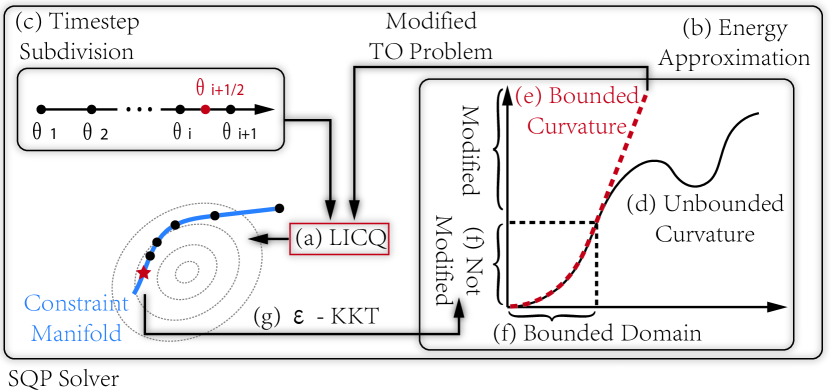
Figure 1: The sketch of convergence proof for our white-box TO solver, built on top of the SQP solver framework. Key to the convergence of SQP to a feasible solution lies in the satisfaction of LICQ (a). We use two techniques to ensure the satisfaction of LICQ. First, we approximate the potential energy (b) and introduce penalty functions for hard constraints, leading to an approximate TO problem. Second, we introduce an adaptive timestep subdivision scheme (c). The main goal of our approximation is to regularize the unbounded curvature (d) and derive modified potential energies and penalty functions with bounded curvature (e, red curve). A typical strategy to remove such unbounded curvature is to introduce piecewise functions that keep the energy unmodified in a bounded domain (f) and replace the energy with a smoother model in the unbounded domain. After SQP returns a feasible solution satisfying the $\epsilon$-perturbed KKT condition to the approximate TO (g), we show that the energy level of the generated feasible solution falls inside the bounded, unmodified domain of our approximate energy (f). Therefore, it satisfies the $\epsilon$-perturbed KKT condition of the original TO problem.

3 Feasible and Stable Solution of Approximate TO

In this section, we propose a perturbed version of Equation 1, whose solution can approximate the true solution up to arbitrary user-specified precision (Section 3.1). A key parameter in our approximate model is $L_{2}$ of Assumption 3.2, which controls both the curvature bound and the discrepancy between our modified and the original dynamic system (Section 5.1). Next, we show in Lemma 2 that our approximation combined with small timestep sizes immediately lead to the satisfaction of LICQ. With LICQ, we then show in Section 3.2 that the SQP solver endows global convergence (Theorem 3.8), when working with adaptive timestep subdivision.

3.1 Curvature-bounded Relaxation

Our idea is to adopt the penalty function for all the hard constraints. We denote the penalty function for the $j$th equality (resp. inequality) constraint as $\bar{h}_{j}^{e}$ (resp. $\bar{h}_{j}^{i}$), essentially transforming Equation 1 into an unconstrained optimization:

$$\theta_{i}\in\underset{\theta_{i}}{\text{argmin}}\;\bar{E}_{i}(\theta_{i},\theta_{\gamma(i)},\theta_{\gamma^{2}(i)},u_{\iota(i)},L_{2})$$ (4)

$$\triangleq\frac{1}{2\delta_{i}^{2}}\left\|\theta_{i}-(1+\delta_{i}/\delta_{\gamma(i)})\theta_{\gamma(i)}+(\delta_{i}/\delta_{\gamma(i)})\theta_{\gamma^{2}(i)}\right\|_{M}^{2}+\bar{P}(\theta_{i},u_{\iota(i)},L_{2})$$

$$\bar{P}(\theta_{i},u_{\iota(i)},L_{2})\triangleq\bar{p}(\theta_{i},L_{2})-g^{T}\theta_{i}+b(\theta_{i},u_{\iota(i)})+\sum_{j}\bar{h}_{j}^{e}(h_{j}^{e}(\theta_{i}),L_{2})+$$

$$\sum_{j}\bar{h}_{j}^{i}(h_{j}^{i}(\theta_{i}),L_{2}),$$

where we further introduce an approximate version of the potential energy, denoted as $\bar{p}$. The goal of our approximation is to achieve both weakly-convex and Lipschitz gradient continuity property of $\bar{P}$ in $\theta_{i}$ defined below:

Definition 3.1

(i) A function, say $\bar{P}(\theta_{i},u_{\iota(i)},L_{2})$, is $L$-weakly convex in $\theta_{i}$ if the function $\bar{P}(\theta_{i},u_{\iota(i)},L_{2})+L/2\|\theta_{i}\|^{2}$ is convex in $\theta_{i}$. (ii) The function is $L$-gradient continuous if $\|{\partial{\bar{P}(\theta_{i},u_{\iota(i)},L_{2})}}/{\partial{\theta_{i}}}-{\partial{\bar{P}(\theta_{i}^{\prime},u_{\iota(i)},L_{2})}}/{\partial{\theta_{i}^{\prime}}}\|\leq L\|\theta_{i}-\theta_{i}^{\prime}\|$ for any $\theta_{i},\theta_{i}^{\prime}$. (iii) If both properties hold, we call it $L$-curvature bounded (in $\theta_{i}$).

Remark 2

As in Definition 3.1, we only consider curvature bound with respect to parameter $\theta_{i}$, instead of other parameters, e.g. $u_{\iota(i)}$.

As the name suggests, the two properties bound the curvature of the twice differentiable function $\bar{P}$ from both below and above. We introduce the additional parameter $L_{2}$ to control both bounds. Our relaxation would essentially modify the dynamic system under consideration. Therefore, we need a technique to bound the accuracy of our relaxation. To this end, we introduce the following assumption:

Assumption 3.2

For $\bar{p}(\theta_{i},L_{2}),\bar{h}_{j}^{e}(h_{j}^{e}(\theta_{i}),L_{2}),\bar{h}_{j}^{i}(h_{j}^{i}(\theta_{i}),L_{2})$, we assume:

1. All are $\text{poly}(L_{2})$-curvature bounded, i.e. the bound is a polynomial of $L_{2}$.

2. All are twice differentiable in $\theta_{i}$.

3. All second derivatives are locally Lipschitz continuous.

4. $p\geq 0$ for all $\theta_{i}$ and $\bar{p}=p$ when $\bar{p}\leq L_{2}$.

5. $\bar{h}_{j}^{e}(x,L_{2})$ is monotonic in $|x|$, $\underset{x}{\min}\bar{h}_{j}^{e}=0$, and $\bar{h}_{j}^{e}(x,L_{2})=L_{2}$ when $|x|=1/L_{2}$.

6. $\bar{h}_{j}^{i}(x,L_{2})$ is monotonic in $\underset{}{\max}(1/L_{2}-x,0)$, $\underset{x}{\min}\bar{h}_{j}^{i}=0$, and $\bar{h}_{j}^{i}=L_{2}$ when $x=0$.

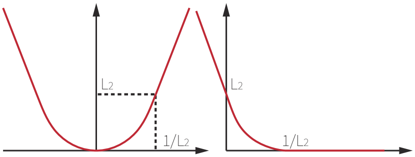
Figure 2: Our penalty function for the equality constraint ($\bar{h}_{j}^{e}$ on the left) and the inequality constraint ($\bar{h}_{j}^{i}$ on the right) ensures their sufficient satisfaction.

Intuitively, Assumption 3.2 formalizes our construction of the approximate dynamic system illustrated in Figure 1. Specifically, (i) ensures the curvature is bounded, which is essential to satisfy LICQ. (ii) and (iii) ensure the minimal requirements on the function smoothness for the well-definedness of SQP. (iv) formalizes the requirement that our dynamic system is only modified in the bounded domain, i.e. when $p\leq L_{2}$. Finally, (v) and (vi) ensures the sufficient satisfaction of (in)equality constraints. As illustrated in Figure 2, if we set $L_{2}=1/\epsilon$ for some user-specified error bound $\epsilon$, then we must have $|h_{j}^{e}|\leq\epsilon$ and $h_{j}^{i}\geq 0$ when $\bar{h}_{j}^{e}(h_{j}^{e},L_{2})\leq L_{2}$ and $\bar{h}_{j}^{i}(h_{j}^{i},L_{2})\leq L_{2}$.

Remark 3

As a key feature in Assumption 3.2, we only require the composite function $\bar{h}_{j}^{e}\circ h_{j}^{e}$ (resp. $\bar{h}_{j}^{i}\circ h_{j}^{i}$) to be twice differentiable, while the individual function $h_{j}^{e}$ (resp. $h_{j}^{i}$) is not necessarily twice differentiable. This is very convenient for modeling non-differentiable collision and contact constraint [15], which we will show in Section 4.3.

Assumption 3.3

For all $\theta_{i}\in\mathcal{C}$ and $u_{\iota(i)}\in\mathcal{X}$, $b(\theta_{i},u_{\iota(i)})$ satisfy Assumption 3.2 (i)-(iii) and $\left\|\partial^{2}{b}/\partial{\theta_{i}}\partial{u_{\iota(i)}}\right\|$ is uniformly upper-bounded.

To motivate the reasoning behind our relaxation, we establish several important consequences of curvature bounds. The following result is an convenient property that can be verified directly:

Lemma 1

(i) Assumption 3.2 (i)-(iii) are closed under summation; (ii) Under Assumption 3.2 and 3.3, $\bar{P}$ and $\bar{E}_{i}$ are $\text{poly}(L_{2})$-curvature-bounded.

Lemma 1 implies that we can design our relaxation separately for each term of the energy or constraint without violating Assumption 3.2, which is a great convenience for practical algorithm designers. In the follow-up analysis, we will use three related matrices defined below:

$$\nabla_{\theta_{\star}}\Lambda\triangleq\left(\begin{array}[]{c}\vdots\\ \frac{\partial{\bar{E}_{\gamma^{2}(N)}}}{\partial{\theta_{\gamma^{2}(N)}}}\\ \frac{\partial{\bar{E}_{\gamma(N)}}}{\partial{\theta_{\gamma(N)}}}\\ \frac{\partial{\bar{E}_{N}}}{\partial{\theta_{N}}}\end{array}\right)\quad\nabla_{\theta_{\star}u}\Lambda\triangleq\left(\begin{array}[]{cccc}\ddots&&&\\ &\frac{\partial^{2}{\bar{E}_{\gamma^{2}(N)}}}{\partial{\theta_{\gamma^{2}(N)}}\partial{u_{\iota\gamma^{2}(N)}}}&&\\ &&\frac{\partial^{2}{\bar{E}_{\gamma(N)}}}{\partial{\theta_{\gamma(N)}}\partial{u_{\iota\gamma(N)}}}&\\ &&&\frac{\partial^{2}{\bar{E}_{N}}}{\partial{\theta_{N}}\partial{u_{\iota(N)}}}\end{array}\right)$$ (5)

$$\nabla_{\theta_{\star}\theta}\Lambda\triangleq\left(\begin{array}[]{cccccc}\ddots&&&&&\\ &\frac{\partial^{2}{\bar{E}_{\gamma^{2}(N)}}}{\partial{\theta_{\gamma^{2}(N)}}\partial{\theta_{\gamma^{4}(N)}}}&\frac{\partial^{2}{\bar{E}_{\gamma^{2}(N)}}}{\partial{\theta_{\gamma^{2}(N)}}\partial{\theta_{\gamma^{3}(N)}}}&\frac{\partial^{2}{\bar{E}_{\gamma^{2}(N)}}}{\partial{\theta_{\gamma^{2}(N)}}^{2}}&&\\ &&\frac{\partial^{2}{\bar{E}_{\gamma(N)}}}{\partial{\theta_{\gamma(N)}}\partial{\theta_{\gamma^{3}(N)}}}&\frac{\partial^{2}{\bar{E}_{\gamma(N)}}}{\partial{\theta_{\gamma(N)}}\partial{\theta_{\gamma^{2}(N)}}}&\frac{\partial^{2}{\bar{E}_{\gamma(N)}}}{\partial{\theta_{\gamma(N)}}^{2}}&\\ &&&\frac{\partial^{2}{\bar{E}_{N}}}{\partial{\theta_{N}}\partial{\theta_{\gamma^{2}(N)}}}&\frac{\partial^{2}{\bar{E}_{N}}}{\partial{\theta_{N}}\partial{\theta_{\gamma(N)}}}&\frac{\partial^{2}{\bar{E}_{N}}}{\partial{\theta_{N}}^{2}}\end{array}\right).$$

We further use subscripts to conveniently denote the block entries in these matrices. For example, $\nabla_{\theta_{\star}\theta}\Lambda_{i}$ extracts the $i$th block row of $\nabla_{\theta_{\star}\theta}\Lambda$ and $\nabla_{\theta_{\star}\theta}\Lambda_{ij}$ extracts the $ij$th block of $\nabla_{\theta_{\star}\theta}\Lambda$.

Lemma 2

Suppose $\bar{P}$ is $L$-curvature-bounded and $\delta_{i}<\sqrt{\sigma_{\min}(M)/L}$, then Equation LABEL:eq:EOMApprox is strongly convex in $\theta_{i}$ and the solution of Equation LABEL:eq:EOMApprox is unique.

Lemma 2 If the given condition holds, then the Hessian of $\bar{E}_{i}$ is bounded away from singularity as:

$$\nabla_{\theta_{\star}}\Lambda_{i}=\frac{M}{\delta_{i}^{2}}+\frac{\partial^{2}{\bar{P}(\theta_{i},u_{\iota(i)},L_{2})}}{\partial{\theta_{i}}^{2}}\succeq\frac{M}{\delta_{i}^{2}}-LI\succeq\left[\frac{\sigma_{\min}(M)}{\delta_{i}^{2}}-L\right]I\succ 0,$$

so the function $\bar{E}_{i}$ is strongly convex and the solution is unique. Here we use $\sigma_{\min}$ (resp. $\sigma_{\max}$) to denote the smallest (resp. largest) singular value. Lemma 2 indicates the backward time-integration is always feasible under sufficiently small timestep size bounded away from zero. Lemma 2 also leads to the following key observation:

Corollary 1

(i) Under the same assumption as Lemma 2, the function $\Lambda_{i}(\theta_{i})\triangleq\|\nabla_{\theta_{\star}}\Lambda_{i}\|^{2}/2$ satisfies the Polyak-Lojasiewicz (PL) condition [22]; if the assumption in Lemma 2 holds for all $i$, then (ii) $\sigma_{\min}(\nabla_{\theta_{\star}\theta}\Lambda)$ is bounded away from zero and (iii) the accumulated function $\Lambda(\theta)\triangleq\sum_{i}\Lambda_{i}$ also satisfies the PL condition.

Corollary 1 (i) Indeed, we have the global minima of this function being zero and we have the following bound on the gradient-norm:

$$\left\|\frac{\partial{\Lambda_{i}}}{\partial{\theta_{i}}}\right\|^{2}=\left\|\nabla_{\theta_{\star}\theta}\Lambda_{ii}\nabla_{\theta_{\star}}\Lambda_{i}\right\|^{2}\geq\left[\frac{\sigma_{\min}(M)}{\delta_{i}^{2}}-L\right]^{2}\left\|\nabla_{\theta_{\star}}\Lambda_{i}\right\|^{2},$$

which is exactly the PL condition. For (ii), we have the following similar result:

$$\|\nabla\Lambda\|^{2}=\left\|\nabla_{\theta_{\star}\theta}\Lambda^{T}\nabla_{\theta_{\star}}\Lambda\right\|^{2}\geq\sigma_{\min}(\nabla_{\theta_{\star}\theta}\Lambda)^{2}\left\|\nabla_{\theta_{\star}}\Lambda\right\|^{2}.$$

We see that diagonal entries of $\nabla_{\theta_{\star}\theta}\Lambda$ are all positive definite so it is non-singular, but we still need to bound the singular value away from zero. By [19], we have the following bound:

$$\sigma_{\min}(\nabla_{\theta_{\star}\theta}\Lambda)=\frac{1}{\|\nabla_{\theta_{\star}\theta}\Lambda^{-1}\|}\geq\frac{(\alpha+2)\beta}{\sqrt{(\alpha+1)^{2|\mathcal{D}||\mathcal{C}|}+2|\mathcal{D}||\mathcal{C}|(\alpha+2)-1}}$$ (6)

$$\alpha\triangleq\underset{m<n}{\max}\frac{|[\nabla_{\theta_{\star}\theta}\Lambda]_{nm}|}{|[\nabla_{\theta_{\star}\theta}\Lambda]_{nn}|}\;\text{and}\;\beta\triangleq\underset{n}{\min}|[\nabla_{\theta_{\star}\theta}\Lambda]_{nn}|,$$

where we use $[\bullet]_{mn}$ to denote the $mn$th entry (instead of block entry) of a matrix. Our next goal is to upper bound $\alpha$ and lower bound $\beta$. Since the diagonal entries of the positive definite matrix is lower-bounded by the smallest eigenvalue, we have:

$$\beta\geq\underset{i}{\min}\left[\frac{\sigma_{\min}(M)}{\delta_{i}^{2}}-L\right]>0,$$

by using Lemma 2. To upper bound $\alpha$, we consider two cases with the off-diagonal entry $[\nabla_{\theta_{\star}\theta}\Lambda]_{nm}$. If the entry belongs to some diagonal matrix of $\nabla_{\theta_{\star}\theta}\Lambda$, then it takes the form:

$$\left[\nabla_{\theta_{\star}}\Lambda_{i}\right]_{nm}=\left[\frac{M}{\delta_{i}^{2}}+\frac{\partial^{2}{\bar{P}}}{\partial{\theta_{i}}^{2}}\right]_{nm}\leq\sigma_{\max}\left[\frac{M}{\delta_{i}^{2}}+\frac{\partial^{2}{\bar{P}}}{\partial{\theta_{i}}^{2}}\right]\leq\frac{\sigma_{\max}(M)}{\delta_{i}^{2}}+L,$$

where we used the fact that the entry of positive definite matrices are bounded by their eigenvalues and $\bar{P}$ is $L$-curvature bounded. If the entry belongs to some non-zero off-diagonal matrices, then there can only be one of the following cases:

$$\nabla_{\theta_{\star}\theta}\Lambda_{i\gamma^{2}(i)}=\frac{M}{\delta_{i}\delta_{\gamma(i)}}\;\text{and}\;\nabla_{\theta_{\star}\theta}\Lambda_{i\gamma(i)}=\frac{(1+\delta_{i}/\delta_{\gamma(i)})M}{\delta_{i}^{2}}.$$

Combining the two cases, we have the following upper bound of $\alpha$:

$$\alpha\leq\left[\underset{i}{\max}\left[\frac{1}{\delta_{i}^{2}},\frac{1}{\delta_{i}\delta_{\gamma(i)}},\frac{1+\delta_{i}/\delta_{\gamma(i)}}{\delta_{i}^{2}}\right]\sigma_{\max}(M)+L\right]/{\underset{i}{\min}\left[\frac{\sigma_{\min}(M)}{\delta_{i}^{2}}-L\right]}.$$

Put together, we have $\sigma_{\min}(\nabla_{\theta_{\star}\theta}\Lambda)$ is bounded away from zero, so (ii) and (iii) holds. The condition (ii) above immediately implies LICQ, i.e., that the local gradient descend algorithm applied to $\Lambda(\theta)$ will linearly converge to zero, which essentially finds the feasible solution to Equation LABEL:eq:EOMApprox by Lemma 2. As a result, we can replace Equation LABEL:eq:EOMApprox with an equivalent condition of vanishing gradient and reformulate Equation 3 as the following equality constrained NLP:

$$\underset{\theta,u_{i}\in\mathcal{X}}{\text{argmin}}\;O(\theta,u)\quad\text{s.t.}\quad\nabla_{\theta_{\star}}\Lambda=0.$$ (7)

Finally, note that $\Lambda(\theta)$ is one of the exact penalty functions that SQP algorithm would use to solve Equation 7. In summary, the lower bound of $\sigma_{min}(\nabla_{\theta_{\star}\theta}\Lambda)$ indicates the feasibility of SQP. In the next section, we will further show that the upper bound of $\sigma_{max}(\nabla_{\theta_{\star}\theta}\Lambda)$ indicates the stability of SQP and we establish this bound for now.

Lemma 3

Under Assumption 3.2, 3.3, (i) $\sigma_{\max}(\nabla_{\theta_{\star}\theta}\Lambda)$ is upper bounded; (ii) $\sigma_{\max}(\nabla_{\theta_{\star}u}\Lambda)$ is upper bounded.

Lemma 3 (i) We propose a very pessimistic estimate that:

$$\sigma_{\max}(\nabla_{\theta_{\star}\theta}\Lambda)=\|\nabla_{\theta_{\star}\theta}\Lambda\|\leq \sum_{i}\left[\left\|\nabla_{\theta_{\star}\theta}\Lambda_{i\gamma^{2}(i)}\right\|+\left\|\nabla_{\theta_{\star}\theta}\Lambda_{i\gamma(i)}\right\|+\left\|\nabla_{\theta_{\star}}\Lambda_{i}\right\|\right]$$

$$\leq |\mathcal{D}|\left[\underset{i}{\max}\left[\frac{1}{\delta_{i}^{2}}+\frac{1}{\delta_{i}\delta_{\gamma(i)}}+\frac{1+\delta_{i}/\delta_{\gamma(i)}}{\delta_{i}^{2}}\right]\sigma_{\max}(M)+L\right],$$

where we used the estimates of the norm of three blocks in each row from Lemma 2.

(ii) The norm of diagonal block matrix is bounded by the norm of the maximal block entry, but each diagonal block entry $\left\|\partial^{2}{b}/\partial{\theta_{i}}\partial{u_{\iota(i)}}\right\|$ is uniformly upper bounded, so $\sigma_{\max}(\nabla_{\theta_{\star}u}\Lambda)=\|\nabla_{\theta_{\star}u}\Lambda\|$ attains the same upper bound.

3.2 Globally Convergent, Feasible, and Stable SQP

In this section, we aim to design an SQP algorithm that is guaranteed to converge to a stationary and feasible solution of Equation 7 in a numerically stable manner. SQP algorithm is a well-known framework for solving NLP and its theoretical properties are well-documented, e.g., in [7]. Let us consider the equality constrained NLP Equation 7. The main idea of SQP is to use some merit function to monitor the progress of problem solving, of which a typical merit function used in our analysis is the following $L_{1}$-merit function:

$$\psi_{\rho}(\theta,u)=O+\rho\|\nabla_{\theta_{\star}}\Lambda\|_{1},$$ (8)

where the first term ensures stationarity and the second term penalizes constraint violation. The reason we use the $L_{1}$- instead of $L_{2}$-merit function is because the convergence analysis of SQP with $L_{2}$-merit function requires $3$rd-order derivatives of $\bar{P}$ to be available, which unnecessarily complicates the design of function models. SQP algorithm works by deriving the descendent directions of $\psi_{\rho}$ and ensuring its reduction by various globalization techniques such as line search and trust-region scheme. In our analysis, we consider the descendent direction computed by the following Quadratic Program (QP):

$$\text{QP}^{k}:\begin{cases}\underset{\underset{u_{i}^{k}+d_{u_{i}}^{k}\in\mathcal{X}}{d_{\theta u}^{k}}}{\text{argmin}}\;&[d_{\theta}^{k}]^{T}\frac{\partial{O}}{\partial{\theta}}^{k}+[d_{u}^{k}]^{T}\frac{\partial{O}}{\partial{u}}^{k}+\frac{1}{2}[d_{\theta}^{k}]^{T}H_{\theta}^{k}d_{\theta}^{k}+\frac{1}{2}[d_{u}^{k}]^{T}H_{u}^{k}d_{u}^{k}\\ \text{s.t.}&\nabla_{\theta_{\star}}\Lambda^{k}+\nabla_{\theta_{\star}\theta}\Lambda^{k}d_{\theta}^{k}+\nabla_{\theta_{\star}u}\Lambda^{k}d_{u}^{k}=0\end{cases},$$ (9)

where we use superscript $k$ to denote the solution or function evaluated at the $k$th iteration. $H_{\theta}^{k},H_{u}^{k}$ are selected positive-definite approximate Hessian matrices.

Definition 3.4

The solution of $\text{QP}^{k}$ satisfies its own KKT condition, denoted as $\text{KKT-QP}^{k}$:

$$\text{KKT-QP}^{k}:\begin{cases}0=\frac{\partial{O}}{\partial{\theta}}^{k}+H_{\theta}^{k}d_{\theta}^{k}+[\nabla_{\theta_{\star}\theta}\Lambda^{k}]^{T}\mu_{\theta}^{k}\\ 0=\frac{\partial{O}}{\partial{u}}^{k}+H_{u}^{k}d_{u}^{k}+[\nabla_{\theta_{\star}u}\Lambda^{k}]^{T}\mu_{\theta}^{k}+\mu_{u}^{k}\\ 0=\nabla_{\theta_{\star}}\Lambda^{k}+\nabla_{\theta_{\star}\theta}\Lambda^{k}d_{\theta}^{k}+\nabla_{\theta_{\star}u}\Lambda^{k}d_{u}^{k}\\ u_{i}^{k}+d_{u_{i}}^{k}\in\mathcal{X}\;\text{and}\;\mu_{u_{i}}^{k}\in\partial\mathcal{X}(u_{i}^{k}+d_{u_{i}}^{k})\end{cases},$$

where $\mu_{\theta}^{k}$ (resp. $\mu_{u}^{k}$) is the Lagrangian multiplier corresponding to the physics (resp. control space) constraint.

Over the years, variants of SQP algorithms have been proposed that differ in their assumptions and convergence guarantees. Two common goals of their assumptions are to ensure that the NLP is feasible and the sequence of penalty coefficient $\{\rho^{k}\}$ is bounded, which in turn indicates numerical stability. From Corollary 1, we see that under given $L_{2}$ and sufficiently small timestep sizes, it is always possible to reduce the constraint violation to zero, indicating feasibility. Unfortunately, the appropriate timestep sizes are not known a priori. Therefore, we need to design algorithms to adaptively estimate them.

3.2.1 Adaptive Timestep Subdivision and Constraint Satisfaction

We have already seen from Section 3.1 that the feasibility and stability requires the boundedness of $\nabla_{\theta_{\star}\theta}\Lambda$ away from singularity, which in turn requires sufficiently small timestep size not known a priori. To allow the estimation of timestep sizes, our solver needs to adaptively decide the set of decision variables. As defined in Section 2, we assume that user provides the solver with an initial stepsize $\delta$ (without subscript) and a total number of timesteps $N$, fixing the control horizon to $\delta N$. When the algorithm decides that the timestep size between $\theta_{i}$ and $\theta_{\gamma(i)}$ is too large, we use midpoint subdivision outlined in Algorithm 1. After a finite number of subdivisions, we get a set of decision variables such that $\theta_{i}\in\mathcal{D}$ can take on fractional subscripts and depicts the kinematic state of the system at the time instance $\delta i$. All our notations and results carry over naturally to the subdivided settings with only one modification to the definition of $\iota(i)$, the time index of control signal. Note that although we introduce new $\theta_{i}$ into the decision variables, we do not introduce new $u_{i}$ accordingly and only use the control signals at integer time indices. We assume that all $\theta_{j}$ with $j\in(i-1,i]$ uses the control signal $u_{i}$, i.e., we extend the definition to have $\iota(i)=\lceil i\rceil$. This is a common setting used by all prior model-based control methods to have the control signal updated at a regular time interval independent of the simulator.

Algorithm 1 Subdivide($\mathcal{D},i$)

1:$\theta_{(i+\gamma(i))/2}\leftarrow(\theta_{i}+\theta_{\gamma(i)})/2$

2:$\mathcal{D}\leftarrow\mathcal{D}\cup(\theta_{(i+\gamma(i))/2})$

3:Return $\mathcal{D}$

When sufficient subdivisions are performed, we can utilize the PL condition (Corollary 1) to ensure the satisfaction of constraints up to an arbitrary error bound. This functionality will be used to ensure the numerical stability of our low-level SQP solver. However, the PL-condition requires that $\nabla_{\theta_{\star}\theta}\Lambda$ is uniformly bounded away from zero for all $\theta^{k}$, which is intractable to check. Instead, we only check that the matrix $\nabla_{\theta_{\star}\theta}\Lambda$ is non-singular at the current solution $\theta^{k}$, i.e., the local PL condition. We will show that such local PL condition suffices to ensure the finite termination of constraint satisfaction Algorithm 2. During each iteration, Algorithm 2 first verify that $\nabla_{\theta_{\star}\theta}\Lambda$ is non-singular at the current solution (Line 5). If the verification fails, the algorithm returns immediately with the index of non-singular diagonal block. It then use a Newton’s step to reduce the constraint violation until some positive threshold $L_{4}$ is reached. Finally, globalization is achieved using a line-search technique to ensure the satisfaction of the Wolfe’s first condition by progressively reducing the step size by a factor of $\eta$, a user provided parameter:

$$\Lambda(\theta^{k}+[\eta^{j}]^{k}d_{\theta}^{k})<(1-2\alpha[\eta^{j}]^{k})\Lambda^{k},$$ (10)

with $\eta^{j}$ being the step size and $\alpha\in(0,1)$. Here we denote $[\eta^{j}]^{k}$ as the step size computed at the $k$th iteration. We show that Algorithm 2 terminates within finitely many iterations.

Algorithm 2 Constraint-Solve($\mathcal{D},u_{i}\in\mathcal{X},L_{2},L_{3},L_{4},\eta\in(0,1),\alpha\in(0,1)$)

1:$\theta^{0}\leftarrow\theta$

2:while $k=0,1,2,\cdots$ do

3:     for $\theta_{i}\in\mathcal{D}$ do

4:         if $\sigma_{\min}(\nabla_{\theta_{\star}\theta}\Lambda_{ii}^{k})<L_{3}$ then

5:              Return $\mathcal{D},i$               

6:     if $\|\nabla_{\theta_{\star}}\Lambda^{k}\|_{1}<L_{4}$ then

7:         Return $\mathcal{D},\emptyset$      

8:     $d_{\theta}^{k}\leftarrow-[\nabla_{\theta_{\star}\theta}\Lambda^{k}]^{-1}\nabla_{\theta_{\star}}\Lambda^{k}$

9:     Find smallest $j\in\mathbb{Z}^{+}$ satisfying Equation 10

10:     $\theta^{k+1}\leftarrow\theta^{k}+[\eta^{j}]^{k}d_{\theta}^{k}$

Lemma 4

Taking Assumption 3.2, 3.3, suppose all $\|\theta^{k}\|$ are bounded by some $L_{12}$, then any $[\eta^{j}]^{k}<\bar{\eta}(L_{12})$ satisfy Equation 10, where $\bar{\eta}(L_{12})$ is a positive function of $L_{12}$.

Lemma 4 By the non-singularity check in Line 5 and Equation LABEL:eq:SigmaMinBound from Corollary 1, we know that for all $k$:

$$\sigma_{\min}(\nabla_{\theta_{\star}\theta}\Lambda^{k})\geq\frac{(\bar{\alpha}+2)L_{3}}{\sqrt{(\bar{\alpha}+1)^{2|\mathcal{D}||\mathcal{C}|}+2|\mathcal{D}||\mathcal{C}|(\bar{\alpha}+2)-1}}\triangleq\underline{\sigma_{\min}}(\nabla_{\theta_{\star}\theta}\Lambda)$$

$$\bar{\alpha}\triangleq\left[\underset{i}{\max}\left[\frac{1}{\delta_{i}^{2}},\frac{1}{\delta_{i}\delta_{\gamma(i)}},\frac{1+\delta_{i}/\delta_{\gamma(i)}}{\delta_{i}^{2}}\right]\sigma_{\max}(M)+\text{poly}(L_{2})\right]/L_{3}.$$

Now by Weyl’s inequality [20, Theorem 4.3.1], $\sigma_{\min}(\nabla_{\theta_{\star}\theta}\Lambda)$ is a locally Lipschitz function of $\theta$, so in the bounded domain, we can denote its bound-dependent Lipschitz constant as $L_{\sigma}(L_{12})$ such that:

$$|\sigma_{\min}(\nabla_{\theta_{\star}\theta}\Lambda(\theta))-\sigma_{\min}(\nabla_{\theta_{\star}\theta}\Lambda^{k})|\leq L_{\sigma}(L_{12})\|\theta-\theta^{k}\|.$$

Combined, we can bound the singular value away from zero in a small neighborhood around $\theta_{k}$ with fixed radius, specifically:

$$\sigma_{\min}(\nabla_{\theta_{\star}\theta}\Lambda(\theta))\geq\underline{\sigma_{\min}}(\nabla_{\theta_{\star}\theta}\Lambda)/2,$$

for any $\|\theta-\theta^{k}\|<\underline{\sigma_{\min}}(\nabla_{\theta_{\star}\theta}\Lambda)/(2L_{\sigma}(L_{12}))$. To ensure that $\theta$ after line search belongs to this small neighborhood, we need to upper bound $d_{\theta}^{k}$ as follows:

$$\|d_{\theta}^{k}\|\leq \|[\nabla_{\theta_{\star}\theta}\Lambda^{-1}]^{k}\|\|\nabla_{\theta_{\star}}\Lambda^{k}\|$$ (11)

$$\leq \|\nabla_{\theta_{\star}}\Lambda^{k}\|/\underline{\sigma_{\min}}(\nabla_{\theta_{\star}\theta}\Lambda)\leq\|\nabla_{\theta_{\star}}\Lambda^{0}\|/\underline{\sigma_{\min}}(\nabla_{\theta_{\star}\theta}\Lambda).$$

This implies that $\theta^{k}+[\eta^{j}]^{k}d_{\theta}^{k}$ belongs to the above neighborhood of $\theta^{k}$ if:

$$[\eta^{j}]^{k}\leq\underline{\sigma_{\min}}(\nabla_{\theta_{\star}\theta}\Lambda)^{2}/(2L_{\sigma}(L_{12})\|\nabla_{\theta_{\star}}\Lambda^{0}\|),$$ (12)

and we assume Equation 12 in the analysis below.

Next, we consider the function $\Lambda$ as a function of $\theta$ only with gradient being $\nabla_{\theta_{\star}\theta}\Lambda^{T}\nabla_{\theta_{\star}}\Lambda$. Since $\nabla_{\theta_{\star}\theta}\Lambda$ is locally Lipschitz by Assumption 3.2, 3.3 and $\nabla_{\theta_{\star}}\Lambda$ is differentiable and thus locally Lipschitz, their product is locally Lipschitz. We denote its bound-dependent L-modulus as $L(L_{12})$. We can estimate the function value bound after line search by [29, Lemma 1.2.3]:

$$\Lambda(\theta^{k}+[\eta^{j}]^{k}d_{\theta}^{k})\leq \Lambda^{k}-2[\eta^{j}]^{k}\Lambda^{k}+\frac{L(L_{12})}{2}([\eta^{j}]^{k})^{2}\|d_{\theta}^{k}\|^{2}$$

$$\leq \Lambda^{k}-2[\eta^{j}]^{k}\Lambda^{k}+\frac{L(L_{12})}{\underline{\sigma_{\min}}(\nabla_{\theta_{\star}\theta}\Lambda)^{2}}([\eta^{j}]^{k})^{2}\Lambda^{k}.$$

To satisfy the Wolfe’s condition, we only need:

$$[\eta^{j}]^{k}\leq 2(1-\alpha)\underline{\sigma_{\min}}(\nabla_{\theta_{\star}\theta}\Lambda)^{2}/L(L_{12}).$$

Combining both conditions, we define:

$$\bar{\eta}(L_{12})\triangleq\min\left[\frac{2(1-\alpha)}{L(L_{12})},\frac{1}{(2L_{\sigma}(L_{12})\|\nabla_{\theta_{\star}}\Lambda^{0}\|)}\right]\underline{\sigma_{\min}}(\nabla_{\theta_{\star}\theta}\Lambda)^{2},$$

which is a positive function of $L_{12}$ that bounds the line search step size away from zero.

Lemma 5 (Constraint-Convergence)

Taking Assumption 3.2, Algorithm 2 (i) is well-defined and (ii) terminates after finitely many iterations.

Lemma 5 (i) If the non-singular check in Line 5 fails, the algorithm terminates immediately. Otherwise, the matrix in the Newton’s step is invertible and the line search step size can be found (Lemma 4), so the algorithm is well-defined.

(ii) We prove by contradiction, considering the sequence $\sum_{k}[\eta^{j}]^{k}$ in two cases. Case I: If $\sum_{k}[\eta^{j}]^{k}=\infty$, then by telescoping, we have:

$$2\alpha\sum_{m=0}^{k}[\eta^{j}]^{k}\Lambda^{k}\leq\Lambda^{0}-\Lambda^{k+1}\leq\Lambda^{0}.$$

But this means $\Lambda^{k}$ can get arbitrarily close to zero, leading to finite termination at Line 7. Case II: If $\sum_{k}[\eta^{j}]^{k}<\infty$ then we have a bounded sequence of $\{\theta^{k}\}$ because:

$$\|\theta^{k}\|\leq\|\theta^{0}\|+\sum_{k}[\eta^{j}]^{k}\|d_{\theta}^{k}\|\leq\|\theta^{0}\|+\sum_{k}[\eta^{j}]^{k}\|\nabla_{\theta_{\star}}\Lambda^{0}\|/\underline{\sigma_{\min}}(\nabla_{\theta_{\star}\theta}\Lambda)\triangleq L_{12},$$

where we have used Equation 11 and we define $L_{12}$ exactly as in Lemma 4. (Note that although Lemma 4 assumes bounded $\|\theta^{k}\|$, Equation 11 there does not rely on such assumption.) As a result, we know that each $[\eta^{j}]^{k}\geq\bar{\eta}(L_{12})/\eta$ is uniformly bounded away from zero, so again $\Lambda^{k}$ gets arbitrarily close to zero, leading to finite termination at Line 7. These contradictions prove our result.

3.2.2 Low-level SQP Solver

In the previous section, we only consider the constraint satisfaction problem. In this section, we incorporate the objective function and present our low-level SQP algorithm to solve Equation 7 and prove global convergence, feasibility, and stability. Our technique of proof is slightly modified from [37], where the key idea is to use an additional condition to ensure the boundedness of constraint violation.

Lemma 6

Presuming (i) Assumption 2.1,3.2,3.3; (ii) the check in Line 4 of Algorithm 3 passes; (iii) there exists some $L_{5}>0$ such that:

$$1/L_{5}\leq\sigma_{\min}(H_{\theta u}^{k})\leq\sigma_{\max}(H_{\theta u}^{k})\leq L_{5},$$ (13)

and iv) $\rho^{k}>\underset{i}{\max}\|\mu_{\theta_{i}}^{k}\|+L_{10}$, then $\text{QP}^{k}$ is convex, feasible, and $d_{\theta u}^{k}$ is the descend direction of $\psi_{\rho}$.

Lemma 6 By our choice of $H^{k}$, $\text{QP}^{k}$ is a convex program, so a feasible solution can be found when one exists using e.g. [2]. Since $\mathcal{X}$ is non-empty, we can choose $u_{i}^{k}+d_{u_{i}}^{k}\in\mathcal{X}$ and since $\nabla_{\theta_{\star}\theta}\Lambda^{k}$ is non-singular by Corollary 1, we can then choose $d_{\theta}^{k}$ satisfying the linear constraints, proving feasibility. We next consider the directional derivative of $\psi_{\rho}$ along $d_{\theta u}^{k}$:

$$[D\psi_{\rho}]^{k}$$

$$= [d_{\theta}^{k}]^{T}\frac{\partial{O}}{\partial{\theta}}^{k}+[d_{u}^{k}]^{T}\frac{\partial{O}}{\partial{u}}^{k}+$$

$$\rho^{k}\sum_{i,j\in I_{\neq 0}}[\nabla_{\theta_{\star}}\Lambda_{i}^{k}]_{j}^{T}\left[[\nabla_{\theta_{\star}\theta}\Lambda_{i}^{k}]_{j}d_{\theta}^{k}+[\nabla_{\theta_{\star}u}\Lambda_{i}^{k}]_{j}d_{u}^{k}\right]/|[\nabla_{\theta_{\star}}\Lambda_{i}^{k}]_{j}|+$$

$$\rho^{k}\sum_{i,j\in I_{=0}}|[\nabla_{\theta_{\star}\theta}\Lambda_{i}^{k}]_{j}d_{\theta}^{k}+[\nabla_{\theta_{\star}u}\Lambda_{i}^{k}]_{j}d_{u}^{k}|$$

$$= [d_{\theta}^{k}]^{T}\frac{\partial{O}}{\partial{\theta}}^{k}+[d_{u}^{k}]^{T}\frac{\partial{O}}{\partial{u}}^{k}-\rho^{k}\sum_{i,j\in I_{\neq 0}}|[\nabla_{\theta_{\star}\theta}\Lambda_{i}^{k}]_{j}d_{\theta}^{k}+[\nabla_{\theta_{\star}u}\Lambda_{i}^{k}]_{j}d_{u}^{k}|$$

$$= -[d_{\theta}^{k}]^{T}H_{\theta}^{k}d_{\theta}^{k}-[d_{u}^{k}]^{T}H_{u}^{k}d_{u}^{k}-\rho^{k}\sum_{i,j\in I_{\neq 0}}|[\nabla_{\theta_{\star}}\Lambda_{i}^{k}]_{j}|-\sum_{i,j\in I_{\neq 0}}[\mu_{\theta_{i}}^{k}]^{T}\nabla_{\theta_{\star}}\Lambda_{i}^{k}-[d_{u}^{k}]^{T}\mu_{u}^{k}$$

$$\leq -[d_{\theta}^{k}]^{T}H_{\theta}^{k}d_{\theta}^{k}-[d_{u}^{k}]^{T}H_{u}^{k}d_{u}^{k}-\sum_{i,j\in I_{\neq 0}}|[\nabla_{\theta_{\star}}\Lambda_{i}^{k}]_{j}|(\rho^{k}-\|\mu_{\theta_{i}}^{k}\|)$$

$$\leq -\frac{1}{L_{5}}\|d_{\theta u}^{k}\|^{2}-L_{10}\sum_{i,j\in I_{\neq 0}}|[\nabla_{\theta_{\star}}\Lambda_{i}^{k}]_{j}|=-\frac{1}{L_{5}}\|d_{\theta u}^{k}\|^{2}-L_{10}\|\nabla_{\theta_{\star}}\Lambda^{k}\|_{1}\triangleq[\bar{D}\psi_{\rho}]^{k},$$

where again $[\bullet]_{j}$ indicates the $j$th row of a matrix or vector. Here we define $I_{\neq 0}$ as the index set such that $[\Lambda_{i}^{k}]_{j}\neq 0$ and $I_{=0}$ is the complement. We have also used the fact that $[d_{u}^{k}]^{T}\mu_{u}^{k}\geq 0$ when $\mu_{u_{i}}\in\partial\mathcal{X}(u_{i}^{k}+d_{u_{i}}^{k})$, and we denote $\mu_{\theta_{i}}^{k}$ (resp. $\mu_{u_{i}}^{k}$) as the Lagrangian multiplier for the physics (resp. control space) constraint at time (resp. control) index $i$. We see that for the decrease of $\psi_{\rho}$, $\rho^{k}$ must be lower bounded by the Lagrangian multipliers $\mu_{\theta_{i}}^{k}$. As our next step, we need to upper bound $\{\mu_{\theta_{i}}^{k}\}$, which in turn upper bounds $\{\rho^{k}\}$ and ensures numerical stability.

Lemma 7

Taking the same assumption as Lemma 6. If $u_{i}^{k}\in\mathcal{X}$ and there exists some $L_{6}$ such that $\|\nabla_{\theta_{\star}}\Lambda^{k}\|_{1}\leq L_{6}$, i.e. the constraint violation is uniformly bounded across all iterations, then there exists $L_{6}$-dependent constants $L_{8}(L_{6})$ and $L_{9}(L_{6})$ such that $\|d_{\theta u}^{k}\|\leq L_{8}(L_{6})$ and $\|\mu_{\theta}^{k}\|\leq L_{9}(L_{6})$, respectively.

Lemma 7 We first show that $d_{\theta u}^{k}$ is uniformly bounded. To this end, we first construct a feasible solution denoted as $d_{\theta u}^{\dagger}$. Since $u_{i}^{k}\in\mathcal{X}$ by assumption, setting $d_{u}^{\dagger}=0$ trivially satisfy the last condition of $\text{KKT-QP}^{k}$. We then solve for a feasible $d_{\theta}^{\dagger}=-\nabla_{\theta_{\star}\theta}\Lambda^{-1}\nabla_{\theta_{\star}}\Lambda$. The norm of such a feasible solution is bounded by $\|d_{\theta u}^{\dagger}\|\leq L_{6}/\underline{\sigma_{\min}}(\nabla_{\theta_{\star}\theta}\Lambda)$ where we construct the lower bound $\underline{\sigma_{\min}}(\nabla_{\theta_{\star}\theta}\Lambda)$ using the same arguement in Lemma 4. At this feasible solution, the objective function value is thus bounded by:

$${d_{\theta}^{\dagger}}^{T}\frac{\partial{O}}{\partial{\theta}}^{k}+{d_{u}^{\dagger}}^{T}\frac{\partial{O}}{\partial{u}}^{k}+\frac{1}{2}{d_{\theta}^{\dagger}}^{T}H_{\theta}^{k}d_{\theta}^{\dagger}+\frac{1}{2}{d_{u}^{\dagger}}^{T}H_{u}^{k}d_{u}^{\dagger}$$

$$\leq L_{1}\|d_{\theta u}^{\dagger}\|+\frac{L_{5}}{2}\|d_{\theta u}^{\dagger}\|^{2}\leq L_{1}\frac{L_{6}}{\underline{\sigma_{\min}}(\nabla_{\theta_{\star}\theta}\Lambda)}+\frac{L_{5}}{2}\frac{L_{6}^{2}}{\underline{\sigma_{\min}}(\nabla_{\theta_{\star}\theta}\Lambda)^{2}}\triangleq L_{7}(L_{6}),$$

due to our choice of $H_{\theta u}^{k}$ as in Equation 13. Now for all feasible solutions satisfying $\|d_{\theta u}^{\dagger}\|>\sqrt{L_{1}^{2}L_{5}^{2}+2L_{7}(L_{6})L_{5}}+L_{1}L_{5}\triangleq L_{8}(L_{6})$, we can lower bound the objective function at such solution as:

$${d_{\theta}^{\dagger}}^{T}\frac{\partial{O}}{\partial{\theta}}^{k}+{d_{u}^{\dagger}}^{T}\frac{\partial{O}}{\partial{u}}^{k}+\frac{1}{2}{d_{\theta}^{\dagger}}^{T}H_{\theta}^{k}d_{\theta}^{\dagger}+\frac{1}{2}{d_{u}^{\dagger}}^{T}H_{u}^{k}d_{u}^{\dagger}\geq\frac{1}{2L_{5}}\|d_{\theta u}^{\dagger}\|^{2}-L_{1}\|d_{\theta u}^{\dagger}\|>L_{7}(L_{6}).$$

As a result, no feasible solutions satisfying $\|d_{\theta u}^{\dagger}\|>L_{8}(L_{6})$ can be stationary, proving the uniform boundedness of $d_{\theta u}^{k}$. We then consider the first equation in $\text{KKT-QP}^{k}$, which yields the following bound:

$$\|\mu_{\theta}\|\leq \|{\partial{O}}/{\partial{\theta}}^{k}+H_{\theta}^{k}d_{\theta}\|/\underline{\sigma_{\min}}(\nabla_{\theta_{\star}\theta}\Lambda)$$

$$\leq (L_{1}+L_{5}L_{8}(L_{6}))/\underline{\sigma_{\min}}(\nabla_{\theta_{\star}\theta}\Lambda)\triangleq L_{9}(L_{6}),$$

which yields our desired bound. Note that our Lemma 7 still requires the boundedness of constraint violation. But this can be achieved by introducing an additional safeguard into the line-search scheme to satisfy the following condition as done in [37]:

$$\begin{cases}\psi_{\rho^{k}}(\theta^{k}+[\eta^{j}]^{k}d_{\theta}^{k},u^{k}+[\eta^{j}]^{k}d_{u}^{k})<\psi_{\rho^{k}}^{k}+\alpha[\eta^{j}]^{k}[\bar{D}\psi_{\rho}]^{k}&\text{if }\|\nabla_{\theta_{\star}}\Lambda^{k}\|_{1}\leq L_{4}\\ \begin{rcases}\psi_{\rho^{k}}(\theta^{k}+[\eta^{j}]^{k}d_{\theta}^{k},u^{k}+[\eta^{j}]^{k}d_{u}^{k})<\psi_{\rho^{k}}^{k}+\alpha[\eta^{j}]^{k}[\bar{D}\psi_{\rho}]^{k}\\ \|\nabla_{\theta_{\star}}\Lambda(\theta^{k}+[\eta^{j}]^{k}d_{\theta}^{k},u^{k}+[\eta^{j}]^{k}d_{u}^{k})\|_{1}\leq\|\nabla_{\theta_{\star}}\Lambda^{k}\|_{1}\\ \end{rcases}&\text{otherwise},\end{cases}$$ (14)

with $\eta^{j}$ being the step size and $\alpha\in(0,1)$ ensures the Wolfe’s first condition. We are now ready to present our Algorithm 3 for solving Equation 7 given fixed $L_{2}$, where the only two modifications to a standard SQP framework are the extra safeguard Equation 14 and the adaptive subdivision.

Algorithm 3 SQP-Inner($\mathcal{D},u_{i}\in\mathcal{X},\rho^{0},L_{2},L_{3},L_{4},L_{5},L_{10},\epsilon,\eta\in(0,1),\alpha\in(0,1)$)

1:while $k=0,1,2,\cdots$ do

2:     for $\theta_{i}\in\mathcal{D}$ do

3:         if $\sigma_{\min}(\nabla_{\theta_{\star}\theta}\Lambda_{ii}^{k})<L_{3}$ then

4:              Return $\mathcal{D},u^{k},\rho^{k},i$               

5:     Choose $H_{\theta}^{k}$, $H_{u}^{k}$ satisfying Equation 13

6:     $d_{\theta u}^{k},\mu_{\theta}^{k}\leftarrow\text{QP}^{k}$

7:     if $\|d_{\theta u}^{k}\|<\epsilon/L_{5}\;\text{and}\;\|\nabla_{\theta_{\star}}\Lambda^{k}\|_{1}<\epsilon$ then

8:         Return $\mathcal{D},u^{k},\rho^{k},\emptyset$      

9:     $\rho^{k}\leftarrow\max(\rho^{k},\max_{i}\|\mu_{\theta_{i}}^{k}\|+L_{10})$

10:     Find smallest $j\in\mathbb{Z}^{+}$ satisfying Equation 14

11:     $\theta^{k+1}\leftarrow\theta^{k}+[\eta^{j}]^{k}d_{\theta}^{k}$ and update $\mathcal{D}\leftarrow(\cdots,\theta_{i}^{k+1},\cdots)$

12:     $u^{k+1}\leftarrow\theta^{k}+[\eta^{j}]^{k}d_{u}^{k}$

We are now ready to prove the desired features of Algorithm 3. First, we establish stability.

Theorem 3.5 (Stability)

Taking Assumption 2.1, 3.2, 3.3, and assuming $\|\nabla_{\theta_{\star}}\Lambda^{0}\|_{1}<L_{4}$, Algorithm 3 generates the bounded sequences $\{d_{\theta u}^{k}\}$ and $\{\rho^{k}\}$.

Theorem 3.5 We first show that all $\{u_{i}^{k}\}\subset\mathcal{X}$. Suppose $u_{i}^{k}\in\mathcal{X}$ in the $k$th iteration, then by $\text{KKT-QP}^{k}$, $u_{i}^{k}+d_{u_{i}}^{k}\in\mathcal{X}$, so $u_{i}^{k+1}=u_{i}^{k}+[\eta^{j}]^{k}d_{u_{i}}^{k}\in\mathcal{X}$ due to convexity. Our result holds that $\{u_{i}^{k}\}\subset\mathcal{X}$ by induction and our initial condition. Next, we show that $\|\nabla_{\theta_{\star}}\Lambda^{k}\|_{1}$ is uniformly bounded by considering the condition in Equation 14. Suppose $\|\nabla_{\theta_{\star}}\Lambda^{k+1}\|_{1}>L_{4}$, then we must have $\|\nabla_{\theta_{\star}}\Lambda^{k}\|_{1}\leq L_{4}$ by assumption that $\|\nabla_{\theta_{\star}}\Lambda^{0}\|_{1}<L_{4}$, so we have by Lemma 7:

$$\|\nabla_{\theta_{\star}}\Lambda^{k}\|_{1}\leq \sum_{i,j}\left|[\nabla_{\theta_{\star}}\Lambda_{i}^{k}]_{j}+\int_{\theta^{k},u^{k}}^{\theta^{k+1},u^{k+1}}[\nabla_{\theta_{\star}\theta}\Lambda_{i}]_{j}d\theta+[\nabla_{\theta_{\star}u}\Lambda_{i}]_{j}du\right|$$

$$\leq \sum_{i,j}|[\nabla_{\theta_{\star}}\Lambda_{i}^{k}]_{j}|+\left[\max\left\|\left(\begin{array}[]{cc}{[\nabla_{\theta_{\star}\theta}\Lambda_{i}]_{j}},&{[\nabla_{\theta_{\star}u}\Lambda_{i}]_{j}}\end{array}\right)\right\|\right]\|d_{\theta u}^{k}\|$$

$$\leq L_{4}+|\mathcal{D}||\mathcal{C}|[\sigma_{\max}(\nabla_{\theta_{\star}\theta}\Lambda)+\sigma_{\max}(\nabla_{\theta_{\star}u}\Lambda)]L_{8}(L_{4})\triangleq L_{11},$$

where the first (resp. second) matrix norm is bounded due to Lemma 3 (i) (resp. Lemma 3 (ii)). After this iteration, the following iterations will reduce $\|\nabla_{\theta_{\star}}\Lambda\|_{1}$ until $\|\nabla_{\theta_{\star}}\Lambda\|_{1}\leq L_{4}$ again. Combined, we see that $\|\nabla_{\theta_{\star}}\Lambda\|_{1}$ can never exceed $L_{11}$ and Lemma 7 indicates that $\{d_{\theta u}^{k}\}$ (resp. $\{\rho^{k}\}$) is uniformly upper bounded by $L_{8}(L_{11})$ (resp. $L_{9}(L_{11})+L_{10}$), which is our desired result. Next, we establish the global convergence and feasibility guarantee using a similar argument as in Lemma 5. We consider the accumulated step size $\sum_{k}[\eta^{j}]^{k}$ in two cases. If this sum is unbounded, then we can use the lower bound on the $\psi_{\rho}$ to establish that $\|d_{\theta u}^{k}\|$ gets arbitrarily small. But if this sum is bounded, then $\{\theta^{k}\}$ and $\{u^{k}\}$ are bounded and both $O$ and $\nabla_{\theta_{\star}}\Lambda$ have L-continuous gradients, leading to $\eta^{j}$ being bounded away from zero and $\|d_{\theta u}^{k}\|$ must get arbitrarily small, again. In both cases, we have finite-step termination and we formalize these observations below:

Lemma 8

Under the same assumption as in Theorem 3.5, suppose further that all $\|\theta^{k}\|$ are bounded by some $L_{12}$, then any $[\eta^{j}]^{k}<\bar{\eta}(L_{12})$ satisfy Equation 14, where $\bar{\eta}(L_{12})$ is a positive function of $L_{12}$.

Lemma 8 By our Assumption 2.1 (ii), $\nabla O$ is locally L-continuous. By the boundedness of domain, $O$ is L-gradient continuous along the line segment between $\theta^{k},u^{k}$ and $\theta^{k+1},u^{k+1}$, where we denote the L-modulus as $L(L_{12})$. We can estimate the function value before and after line-search as:

$$O^{k+1}\leq O^{k}+[\eta^{j}]^{k}[d_{\theta}^{k}]^{T}\frac{\partial{O}}{\partial{\theta}}^{k}+[\eta^{j}]^{k}[d_{u}^{k}]^{T}\frac{\partial{O}}{\partial{u}}^{k}+\frac{L(L_{12})}{2}([\eta^{j}]^{k})^{2}\|d_{\theta u}^{k}\|^{2}.$$

Similarly, we consider the $j$th block-row of constraint $\nabla_{\theta_{\star}}\Lambda_{i}^{k}=0$. The derivatives of this constraint is locally L-continuous by our Assumption 3.2 (iii) and thus $\nabla_{\theta_{\star}}\Lambda_{i}^{k}$ is L-gradient continuous on the same line-segment by the boundedness of domain with L-modulus of the $j$th element denoted as $L_{ij}(L_{12})$. The following estimate applies:

$$|[\nabla_{\theta_{\star}}\Lambda_{i}^{k+1}]_{j}|$$

$$\leq \left|[\nabla_{\theta_{\star}}\Lambda_{i}^{k}]_{j}+[\eta^{j}]^{k}\left[[\nabla_{\theta_{\star}\theta}\Lambda_{i}^{k}]_{j}d_{\theta}^{k}+[\nabla_{\theta_{\star}u}\Lambda_{i}^{k}]_{j}d_{u}^{k}\right]\right|+\frac{L_{ij}(L_{12})}{2}([\eta^{j}]^{k})^{2}\|d_{\theta u}^{k}\|^{2}$$

$$= (1-[\eta^{j}]^{k})|[\nabla_{\theta_{\star}}\Lambda_{i}^{k}]_{j}|+\frac{L_{ij}(L_{12})}{2}([\eta^{j}]^{k})^{2}\|d_{\theta u}^{k}\|^{2}.$$

Combined, we can estimate the value of merit function before and after a line search as:

$$\psi_{\rho^{k}}^{k+1}\leq \psi_{\rho^{k}}^{k}+[\eta^{j}]^{k}[d_{\theta}^{k}]^{T}\frac{\partial{O}}{\partial{\theta}}^{k}+[\eta^{j}]^{k}[d_{u}^{k}]^{T}\frac{\partial{O}}{\partial{u}}^{k}$$ (15)

$$-[\eta^{j}]^{k}\rho^{k}\|\nabla_{\theta_{\star}}\Lambda^{k}\|_{1}+\frac{L(L_{12})+\sum_{i,j}L_{ij}(L_{12})}{2}([\eta^{j}]^{k})^{2}\left\|d_{\theta u}^{k}\right\|^{2}$$

$$\leq \psi_{\rho^{k}}^{k}+[\eta^{j}]^{k}[\bar{D}\psi_{\rho}]^{k}+\frac{L(L_{12})+\sum_{i,j}L_{ij}(L_{12})}{2}([\eta^{j}]^{k})^{2}\left\|d_{\theta u}^{k}\right\|^{2}.$$

Let us now consider the two cases in Equation 14. Case I: If $\|\nabla_{\theta_{\star}}\Lambda^{k}\|_{1}\leq L_{4}$, then we only need sufficient decrease of the merit function. Using Equation 15, we derive the following more conservative condition:

$$\psi_{\rho^{k}}^{k+1}\leq\psi_{\rho^{k}}^{k}+[\eta^{j}]^{k}[\bar{D}\psi_{\rho}]^{k}+\frac{L(L_{12})+\sum_{i,j}L_{ij}(L_{12})}{2}([\eta^{j}]^{k})^{2}\left\|d_{\theta u}^{k}\right\|^{2}$$

$$\leq\psi_{\rho^{k}}^{k}+\alpha[\eta^{j}]^{k}[\bar{D}\psi_{\rho}]^{k}$$

$$\Rightarrow\frac{L(L_{12})+\sum_{i,j}L_{ij}(L_{12})}{2}([\eta^{j}]^{k})^{2}\left\|d_{\theta u}^{k}\right\|^{2}\leq[\eta^{j}]^{k}(\alpha-1)[\bar{D}\psi_{\rho}]^{k}$$

$$\overset{\text{(conservative)}}{\Longrightarrow}\frac{L(L_{12})+\sum_{i,j}L_{ij}(L_{12})}{2}([\eta^{j}]^{k})^{2}\left\|d_{\theta u}^{k}\right\|^{2}\leq[\eta^{j}]^{k}\frac{1-\alpha}{L_{5}}\left\|d_{\theta u}^{k}\right\|^{2},$$

which in turn can be satisfied by setting:

$$\bar{\eta}(L_{12})\triangleq 2(1-\alpha)/\left[L_{5}\left[L(L_{12})+\sum_{i,j}L_{ij}(L_{12})\right]\right].$$

Case II: If $\|\nabla_{\theta_{\star}}\Lambda^{k}\|_{1}>L_{4}$, we need to satisfy the additional condition of strict reduction in constraint violation. To satisfy it, we use our estimation of constraint violation to yield the more conservative condition:

$$\|\nabla_{\theta_{\star}}\Lambda^{k+1}\|_{1}\leq(1-[\eta^{j}]^{k})\|\nabla_{\theta_{\star}}\Lambda^{k}\|_{1}+\sum_{i,j}\frac{L_{ij}(L_{12})}{2}([\eta^{j}]^{k})^{2}\|d_{\theta u}^{k}\|^{2}\leq\|\nabla_{\theta_{\star}}\Lambda^{k+1}\|_{1}$$

$$\Rightarrow\sum_{i,j}\frac{L_{ij}(L_{12})}{2}([\eta^{j}]^{k})^{2}\|d_{\theta u}^{k}\|^{2}\leq[\eta^{j}]^{k}\|\nabla_{\theta_{\star}}\Lambda^{k}\|_{1}$$

$$\overset{\text{(conservative)}}{\Longrightarrow}[\eta^{j}]^{k}\leq\|\nabla_{\theta_{\star}}\Lambda^{k}\|_{1}/\left[\sum_{i,j}\frac{L_{ij}(L_{12})}{2}\|d_{\theta u}^{k}\|^{2}\right].$$

To satisfy both conditions in the second case, we thus define:

$$[\eta^{j}]^{k}\leq\bar{\eta}(L_{12})\triangleq\min\left[\frac{2(1-\alpha)}{L_{5}(L(L_{12})+\sum_{i,j}L_{ij}(L_{12}))},\frac{2L_{4}}{L_{8}(L_{11})^{2}\sum_{i,j}L_{ij}(L_{12})}\right],$$

where we use the condition that $\|\nabla_{\theta_{\star}}\Lambda^{k}\|_{1}>L_{4}$ and the fact that $\|d_{\theta}\|<L_{8}(L_{11})$ according to Theorem 3.5. All is proved by combining the two cases.

Definition 3.6

We say a solution $\theta,u$ satisfies the $\epsilon$-perturbed KKT condition of Equation 7 if:

$$\text{KKT-TO-Approx}^{\epsilon}:\begin{cases}\|\frac{\partial{O}}{\partial{\theta}}+\nabla_{\theta_{\star}\theta}\Lambda^{T}\mu_{\theta}\|\leq\epsilon\\ \|\frac{\partial{O}}{\partial{u}}+\nabla_{\theta_{\star}u}\Lambda^{T}\mu_{\theta}+\mu_{u}\|\leq\epsilon\\ u_{i},u_{i}^{\prime}\in\mathcal{X}\;\text{and}\;\|u_{i}-u_{i}^{\prime}\|\leq\epsilon\;\text{and}\;\mu_{u_{i}}\in\partial\mathcal{X}(u_{i}^{\prime})\\ \sqrt{2\Lambda_{i}}\leq\epsilon\\ \end{cases}.$$

Definition 3.6 degenerates to the exact KKT condition of Equation 7 as $\epsilon\to 0$.

Theorem 3.7 (Feasibility-Stationarity)

If we take the same assumption as in Theorem 3.5, Algorithm 3 (i) is well-defined, (ii) terminates after finitely many iterations, and (iii) returns a solution that satisfies $\text{KKT-TO-Approx}^{\epsilon}$ if Line 8 is executed.

Theorem 3.7 (i) Similar to the case with Lemma 5, if the non-singular check in Line 4 fails, the algorithm terminates immediately. Otherwise, the QP sub-problem is feasible (Lemma 6) and the line search step size can be found (Lemma 8), so the algorithm is well-defined.

(ii) From Lemma 6, we know that the $\text{QP}^{k}$ is always solvable. From Lemma 8, we know that $\eta^{j}$ satisfying Equation 14 can be found. Let us now suppose Algorithm 3 does not terminate finitely, then it generates infinite sequences $\{\theta^{k}\}$ and $\{d^{k}\}$. Let us denote $\psi_{\rho^{k}}^{k+1}$ as the merit function evaluated with $\rho^{k}$ at $\theta^{k+1},u^{k+1}$. We now consider two cases.

Case I: If $\sum_{k}[\eta^{j}]^{k}=\infty$, then we have the following estimate of the merit function value by telescoping:

$$\psi_{\rho^{k}}^{k+1}\leq\psi_{\rho^{k}}^{k}+\alpha[\eta^{j}]^{k}[\bar{D}\psi_{\rho}]^{k}$$

$$\Rightarrow \frac{\rho^{k-1}}{\rho^{k}}\psi_{\rho^{k}}^{k+1}\leq\frac{\rho^{k-1}}{\rho^{k}}[\psi_{\rho^{k}}^{k}+\alpha[\eta^{j}]^{k}[\bar{D}\psi_{\rho}]^{k}]$$

$$\leq \psi_{\rho^{k-1}}^{k}+\alpha\frac{\rho^{k-1}}{\rho^{k}}[\eta^{j}]^{k}[\bar{D}\psi_{\rho}]^{k}$$

$$\leq \psi_{\rho^{k-1}}^{k-1}+\alpha[\eta^{j}]^{k-1}[\bar{D}\psi_{\rho}]^{k-1}+\alpha\frac{\rho^{k-1}}{\rho^{k}}[\eta^{j}]^{k}[\bar{D}\psi_{\rho}]^{k}$$

$$\Rightarrow \frac{\rho^{k-2}}{\rho^{k}}\psi_{\rho^{k}}^{k+1}\leq\frac{\rho^{k-2}}{\rho^{k-1}}[\psi_{\rho^{k-1}}^{k-1}+\alpha[\eta^{j}]^{k-1}[\bar{D}\psi_{\rho}]^{k-1}+\alpha\frac{\rho^{k-1}}{\rho^{k}}[\eta^{j}]^{k}[\bar{D}\psi_{\rho}]^{k}]$$

$$\leq \psi_{\rho^{k-2}}^{k-1}+\alpha\frac{\rho^{k-2}}{\rho^{k-1}}[\eta^{j}]^{k-1}[\bar{D}\psi_{\rho}]^{k-1}+\alpha\frac{\rho^{k-2}}{\rho^{k}}[\eta^{j}]^{k}[\bar{D}\psi_{\rho}]^{k}$$

$$\leq \psi_{\rho^{k-2}}^{k-2}+\alpha[\eta^{j}]^{k-2}[\bar{D}\psi_{\rho}]^{k-2}+\alpha\frac{\rho^{k-2}}{\rho^{k-1}}[\eta^{j}]^{k-1}[\bar{D}\psi_{\rho}]^{k-1}+\alpha\frac{\rho^{k-2}}{\rho^{k}}[\eta^{j}]^{k}[\bar{D}\psi_{\rho}]^{k}$$

$$\vdots$$

$$\Rightarrow \frac{\rho^{0}}{\rho^{k}}\psi_{\rho^{k}}^{k+1}\leq\psi_{\rho^{0}}^{0}+\alpha\sum_{m=0}^{k}\frac{\rho^{0}}{\rho^{m}}[\eta^{j}]^{m}[\bar{D}\psi_{\rho}]^{m}.$$

By Assumption 2.1, we know that $\psi_{\rho^{k}}^{k+1}\geq 0$, so we have for any $k$:

$$-\frac{\rho^{0}\alpha}{L_{9}(L_{11})+L_{10}}\sum_{m=0}^{\infty}[\eta^{j}]^{m}[\bar{D}\psi_{\rho}]^{m}\leq-\alpha\sum_{m=0}^{\infty}\frac{\rho^{0}}{\rho^{m}}[\eta^{j}]^{m}[\bar{D}\psi_{\rho}]^{m}\leq\psi_{\rho^{0}}^{0},$$

where we have used Theorem 3.5 in the first inequality. Now as $\sum_{k}[\eta^{j}]^{k}=\infty$, we can get $-[\bar{D}\psi_{\rho}]^{k}$ arbitrarily small for some sufficiently large $k$. By the definition of $[\bar{D}\psi_{\rho}]^{k}$, we know that $\|d_{\theta u}\|^{k}$ and $\|\nabla_{\theta_{\star}}\Lambda^{k}\|_{1}$ both gets arbitrarily small, so Algorithm 3 terminates finitely, leading to a contradiction.

Case II: If $\sum_{k}[\eta^{j}]^{k}<\infty$, then by Theorem 3.5 we have $\|\nabla_{\theta_{\star}}\Lambda^{k}\|\leq\|\nabla_{\theta_{\star}}\Lambda^{k}\|_{1}\leq L_{11}$ and by Lemma 7 we have $\|d_{\theta u}^{k}\|\leq L_{8}(L_{11})$. As a result, all $\|\theta^{k}\|$ and $\|u^{k}\|$ can be bounded by:

$$\|\left(\begin{array}[]{cc}{\theta^{k}},&{u^{k}}\end{array}\right)\|\leq \|\left(\begin{array}[]{cc}{\theta^{0}},&{u^{0}}\end{array}\right)\|+\sum_{m=0}^{k}[\eta^{j}]^{m}\|d_{\theta u}^{m}\|$$

$$\leq \|\left(\begin{array}[]{cc}{\theta^{0}},&{u^{0}}\end{array}\right)\|+\sum_{m=0}^{\infty}[\eta^{j}]^{m}L_{8}(L_{11})\triangleq L_{12}<\infty,$$

where we define $L_{12}$ as claimed in Lemma 8, leading to the fact that the sequence $\{[\eta^{j}]^{k}\}$ is bounded away from zero by $[\eta^{j}]^{k}\geq\bar{\eta}(L_{12})/\eta$, immediately leading to a contradiction.

(iii) The last two conditions in $\text{KKT-TO-Approx}^{\epsilon}$ satisfies trivially by our termination condition and the satisfaction of $\text{KKT-QP}^{k}$ by $d_{\theta u}^{k}$. The first condition of $\text{KKT-QP}^{k}$ yields:

$$\|{\partial{O}}/{\partial{\theta}}^{k}+[\nabla_{\theta_{\star}\theta}\Lambda^{k}]^{T}\mu_{\theta}^{k}\|=\|H_{\theta}^{k}d_{\theta}^{k}\|\leq L_{5}\|d_{\theta}^{k}\|\leq\epsilon,$$

and the second condition follows using the same argument.

3.2.3 High-level SQP Solver

Our final SQP Algorithm 4 combines the benefits of Algorithm 1,  Algorithm 2, and Algorithm 3. Note that the numerical stability of Algorithm 3 relies on the initial constraint violation to be less than $L_{4}$, which can be achieved using Algorithm 2. Further, both Algorithm 2 and Algorithm 3 can terminate by failing the singularity check, where we use Algorithm 1 to subdivide the timestep size and ensure non-singularity.

Algorithm 4 SQP($\mathcal{D},u_{i}\in\mathcal{X},\rho,L_{2},L_{3},L_{4},L_{5},L_{10},\epsilon,\eta\in(0,1),\alpha\in(0,1)$)

1:$i\leftarrow\emptyset$

2:while Not converged do

3:     if $i\neq\emptyset$ then

4:         $\mathcal{D}\leftarrow$Subdivide($\mathcal{D},i$)

5:         $i\leftarrow\emptyset$      

6:     if $\|\nabla_{\theta_{\star}}\Lambda(\theta)\|_{1}\geq L_{4}$ then

7:         $\mathcal{D},i\leftarrow$Constraint-Solve($\mathcal{D},u_{i},L_{2},L_{3},L_{4},\eta,\alpha$)

8:     else

9:         $\mathcal{D},u,\rho,i\leftarrow$SQP-Inner($\mathcal{D},u_{i},\rho,L_{2},L_{3},L_{4},L_{5},L_{10},\epsilon,\eta,\alpha$)

10:         if $i=\emptyset$ then

11:              Return $\mathcal{D},u,\rho$               

Theorem 3.8 (Stability-Feasibility-Stationarity)

Taking Assumption 2.1, 3.2, 3.3, Algorithm 4 (i) is well-defined, (ii) terminates finitely, (iii) generates a bounded sequence $\{\rho^{k}\}$, and (iv) returns a solution satisfying $\text{KKT-TO-Approx}^{\epsilon}$.

Theorem 3.8 The results follow by combining Corollary 1, Lemma 5,  Theorem 3.5, and Theorem 3.7.

4 Curvature-Bounded Relaxation for Practical Energy

Our Assumption 3.2 can be formidable for practitioners to design approximate potential and penalty functions. As illustrated in Figure 3, we demonstrate that several commonly used potential energy terms and constraints bear curvature-bounded relaxations satisfying Assumption 3.2.

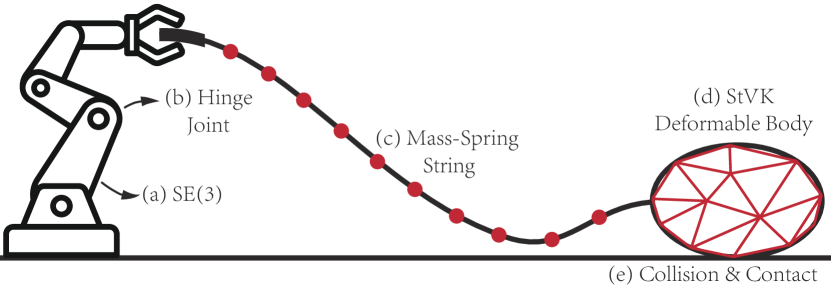
Figure 3: Consider a robot arm dragging a deformable cushion through an elastic string. To model such a scenario, our dynamic system needs to model the $\mathcal{SE}(3)$ constraint for each robot link (a) (Section 4.1) and hinge joint (b) (Section 4.2). The elastic string can be discreted as a mass-spring system (c), using one spring between each pair of red vertices (Section 4.4). And the deforamble cushion can be be modeled using volumetric hyper-elastic energy, such the Saint Venant–Kirchhoff elastic energy (d), using one energy term for each red triangle (Section 4.4). Finally, we need to handle the collisions and contacts (e) between the cushion and the ground (Section 4.3). In our extended paper, we show that all these energy models have curvature-bounded relaxation.

4.1 Rotational Constraint

Probably the most important constraint is that rotation of each robot link is restricted to $\mathcal{SO}(3)$. Since we assume that our configuration $\theta$ is affine-related to the Cartesian space points, so we have to use additional constraint $h^{e}(\theta)=0$ to model $\mathcal{SO}(3)$ constraint. Let us denote by $R\in\mathbb{R}^{3\times 3}$ the rotation matrix of some robot link, which is vectorized as a 9D-subvector of $\theta$. The constraint takes the following form [14]:

$$h^{e}(\theta):\begin{cases}\|R^{T}R-I\|_{F}=0\\ \det(R)=1\\ \end{cases}.$$ (16)

To relax such constraint, we introduce the following penalty function:

Lemma 9

For square matrix $R\in\mathbb{R}^{3\times 3}$ and constant $a>0$, we have $P_{1}(R,a)\triangleq\sqrt{\|R^{T}R-I\|_{F}^{2}+a}$ satisfies Assumption 3.2 (i)-(iii).

Lemma 9 Since the function is smooth, Assumption 3.2 (ii) and (iii) trivially satisfy. For bounded curvature i), we use Einstein’s notation (only for this proof) and define $A(R)\triangleq R^{T}R-I$ and $B(R)\triangleq\|A(R)\|_{F}^{2}$. Each entry of the gradient takes the following form:

$$\frac{\partial{P_{1}}}{\partial{R_{ab}}}=\frac{2[RA(R)]_{ab}}{P_{1}(R,a)},$$

and each entry of the Hessian takes the following form:

$$\frac{\partial^{2}{P_{1}}}{\partial{R_{ab}}\partial{R_{cd}}}=\frac{-4[RA(R)]_{ab}[RA(R)]_{cd}}{P_{1}(R,a)^{3}}+\frac{2[\delta_{ac}[A(R)]_{db}+R_{ad}R_{cb}+R_{am}R_{cm}\delta_{bd}]}{P_{1}(R,a)},$$

where $\delta_{ab}$ is the dirac-delta function. If we can bound each entry of the Hessian, then function $P_{1}$ is curvature-bounded. To this end, we consider two types of terms. First, we consider the following term for any indices $ab$, which can be bounded as:

$$\left|\frac{[A(R)]_{ab}}{P_{1}(R,a)}\right|\leq\left|\frac{[A(R)]_{ab}}{\sqrt{\|A(R)\|_{F}^{2}+a}}\right|\leq\frac{\|A(R)\|_{F}}{\sqrt{\|A(R)\|_{F}^{2}+a}}\leq 1.$$

Second, we consider the following term for any indices $abcd$, which can be bounded as:

$$\left|\frac{R_{ab}R_{cd}}{P_{1}(R,a)}\right|\leq\frac{1}{2}\left|\frac{\|R\|_{F}^{2}}{\sqrt{\|A(R)\|_{F}^{2}+a}}\right|\leq\frac{1}{2}\left|\frac{\sum_{a}([R^{T}R]_{aa}-1)+3}{\sqrt{\sum_{a}([R^{T}R]_{aa}-1)^{2}+a}}\right|\leq\frac{1}{2}\left[3+\frac{3}{\sqrt{a}}\right].$$

We note that the entry $\partial^{2}{P_{1}}/\partial{R_{ab}}\partial{R_{cd}}$ is a polynomial of the above two types of terms, which is thus bounded, so all is proved. We can now use Lemma 9 to design our relaxed function:

Corollary 2

The penalty functions $\bar{h}_{j}^{e}(h_{j}^{e}(\theta_{i}),L_{2})\triangleq L_{2}\sqrt{3L_{2}^{2}\|R^{T}R-I\|_{F}^{2}+1}-L_{2}$ satisfy Assumption 3.2.

Corollary 2 The function satisfies Assumption 3.2 i)-iii) by Lemma 9. When $\|R^{T}R-I\|_{F}\geq 1/L_{2}$, it can be verified that $\bar{h}_{j}^{e}\geq L_{2}$, satisfying Assumption 3.2 (v). Other assumptions are trivial to verify. Finally, we choose not to handle the second constraint $\det(R)=1$, and the reason will be clear later.

4.2 Joint (Limit) Constraint

The joint limit constraint takes a slightly more involved form under maximal coordinates than that in the minimal coordinates. For a hinge joint, we assume their two attaching bodies are denoted using superscript $a,b$ and their rigid transformations are $R^{a},t^{a}$ (resp. $R^{b},t^{b}$). We denote their two attachment points as $R^{a}X^{a}+t^{a}$ (resp. $R^{b}X^{b}+t^{b}$) and two attachment axes as $D^{a}$ (resp. $D^{b}$). Here $X^{a,b},D^{a,b}\in\mathbb{R}^{3}$ are the constant local points and axes of attachment. The joint attachment constraint can then be formulated as:

$$h_{j}^{e}(R^{a},t^{a},R^{b},t^{b})= (R^{a}X^{a}+t^{a})-(R^{b}X^{b}+t^{b})$$

$$h_{j}^{e}(R^{a},R^{b})= R^{a}D^{a}-R^{b}D^{b}.$$

For these attachment constraints, we introduce the quadratic penalty function $\bar{h}_{j}^{e}\triangleq L_{2}^{3}\|h_{j}^{e}\|^{2}$, for which satisfaction of Assumption 3.2 can be trivially verified. Further, if a joint limit is required, then we can introduce two tangent directions $T^{a,b}\in\mathbb{R}^{3}$ and require that:

$$h_{j}^{i}(R^{a},R^{b})=\bar{T}^{2}-\|R^{a}T^{a}-R^{b}T^{b}\|^{2},$$

with $\bar{T}$ being some upper bound of the directional difference. For such constraint, we introduce the following penalty function and verify Assumption 3.2:

$$P_{2}(x,L_{2})=\begin{cases}0&x>1/L_{2}\\ L_{2}(1-L_{2}x)^{3}&x>0\\ L_{2}\sqrt{15(L_{2}x-1/5)^{2}+2/5}&\text{otherwise}\\ \end{cases},$$

We will use the following convenient result:

Lemma 10

For vector $x$ and constants $a,b$ ($b>0$), $P_{3}(x,a,b)\triangleq\sqrt{(\|x\|^{2}+a)^{2}+b}$ satisfies Assumption 3.2 (i)-(iii).

Lemma 10 Since the function is smooth, Assumption 3.2 (ii) and (iii) trivially satisfy. For bounded curvature (i), we note the Hessian matrix has the following closed form:

$$\frac{\partial^{2}{P_{3}}}{\partial{x}^{2}}= \frac{2(\|x\|^{2}+a)}{\sqrt{(\|x\|^{2}+a)^{2}+b}}I+\left[\frac{4}{\sqrt{(\|x\|^{2}+a)^{2}+b}}-\frac{4(\|x\|^{2}+a)^{2}}{\sqrt{(\|x\|^{2}+a)^{2}+b}^{3}}\right]xx^{T},$$

$$\preceq 2I+\left[\frac{4\|x\|^{2}}{\sqrt{(\|x\|^{2}+a)^{2}+b}}-\frac{4(\|x\|^{2}+a)^{2}\|x\|^{2}}{\sqrt{(\|x\|^{2}+a)^{2}+b}^{3}}\right]I$$

$$\preceq 2I+4\left[\frac{(\|x\|^{2}+a)-a}{\sqrt{(\|x\|^{2}+a)^{2}+b}}-\frac{(\|x\|^{2}+a)^{2}}{(\|x\|^{2}+a)^{2}+b}\frac{(\|x\|^{2}+a)-a}{\sqrt{(\|x\|^{2}+a)^{2}+b}}\right]I$$

$$\preceq 2I+8\left[\frac{\|x\|^{2}+a}{\sqrt{(\|x\|^{2}+a)^{2}+b}}+\frac{a}{\sqrt{(\|x\|^{2}+a)^{2}+b}}\right]I$$

$$\preceq 2I+8\left[1+\frac{a}{\sqrt{b}}\right]I,$$

so we have $-LI\preceq{\partial^{2}{P_{3}(x,a,b)}}/{\partial{\theta}^{2}}\preceq LI$ where we define $L=2+(8+8|a|/\sqrt{b})$ and all is proved.

Corollary 3

The penalty functions $\bar{h}_{j}^{i}(h_{j}^{i}(\theta_{i}),L_{2})\triangleq P_{2}(h_{j}^{i}(R^{a},R^{b}),L_{2})$ satisfy Assumption 3.2.

Corollary 3 For the last case in $P_{2}$ where $x\leq 0$, $P_{2}(h_{j}^{i}(R^{a},R^{b}),L_{2})$ takes the same form as $P_{3}$ (up to constant scaling and bias) from Lemma 10 (by defining $x$ equals $R^{a}T^{a}-R^{b}T^{b}$ there), so we can satisfy (i)-(iii). For the second case where $x\in(0,1/L_{2}]$, (ii) and (iii) holds by smoothness and (i) holds by boundedness of domain. In summary, $P_{2}$ satisfies (i)-(iii) globally by direct verification at case boundaries where $x=0,1/L_{2}$. Taking $h_{j}^{i}=0$, we have $\bar{h}_{j}^{i}=L_{2}$ and the function $P_{2}$ is monotonic in $x$, so vi) satisfies.

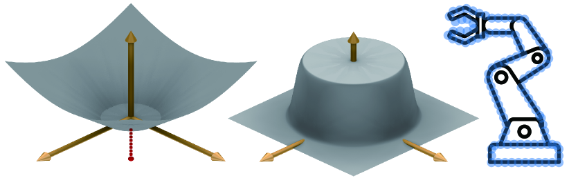
Figure 4: Illustration of the collision penalty using a simple 2D example with a circle and a point. Our penalty smooths the non-differentiable collision constraint. Left: the non-differentiable collision constraint $h^{i}_{j}$ formulated as the distance (red dashed line). Middle: the corresponding collision penalty value $\bar{h}^{i}_{j}$. Right: Our theoretical framework can scale to arbitrarily complex geometries via sphere sampling (blue circles).

4.3 Collision and Contact Constraint

Collision and contact constraints are central to most robot locomotion skills. Incorporating them into the TO formulations have been a long-standing topic in robotic research such as [33, 36, 48]. To this end, we need to deal with the challenge that collision constraints are non-differentiable. Indeed, the collision constraint is formulated using the distance function between two geometric objects, which is singular when the objects are exactly in touch [31, 15]. We tackle this difficulty using our Remark 3, i.e., we design the composite function $\bar{h}_{j}^{i}\circ h_{j}^{i}$ to be twice differentiable, even when $h_{j}^{i}$ is not. We assume that collision constraints take the following form:

$$h_{j}^{i}(\theta_{i})=\text{dist}(C^{a}(\theta_{i}),C^{b}(\theta_{i}))-\epsilon_{r},$$

where we denote $C^{a}$ and $C^{b}$ as the position of two objects that are affine related to $\theta_{i}$ and $\epsilon_{r}>0$ is some positive safe distance. Here we adopt the set-based definition for the distance function dist, i.e., $\text{dist}(C^{a},C^{b})=\inf\{\text{dist}(x,y)|x\in C^{a}\;\text{and}\;y\in C^{b}\}$. The distance function is singular and non-differentiable when it is close to zero, but twice-differentiable otherwise. To workaround such singularity, we could introduce the following clamp function:

$$P_{4}(x,L_{2})=$$

$$\begin{cases}0&x>1/L_{2}\\ L_{2}(1-L_{2}x)^{3}&x>2/(3L_{2})\\ -1296L_{2}^{6}x^{5}+3249L_{2}^{5}x^{4}-3137L_{2}^{4}x^{3}+1451L_{2}^{3}x^{2}-323L_{2}^{2}x+779L_{2}/27&x>1/(3L_{2})\\ L_{2}&\text{otherwise}\\ \end{cases},$$

and define our relaxed penalty function as:

$$\bar{h}_{j}^{i}(h_{j}^{i}(\theta_{i}),L_{2})=\begin{cases}P_{4}(h_{j}^{i}(\theta_{i}),L_{2})&h_{j}^{i}(\theta_{i})>0\\ L_{2}&\text{otherwise}\end{cases}.$$ (17)

Intuitively, we smooth the distance function when the two objects $C^{a},C^{b}$ get too close to each other. A visualization of the penalty function with a 2D example in shown in Figure 4. We can now establish Assumption 3.2 under some mild assumptions on the distance function:

Corollary 4

Suppose the distance function $\text{dist}(C^{a},C^{b})$ between $C^{a}$ and $C^{b}$ is (i) continuous and (ii) twice differentiable with bounded and locally Lipschitz first/second derivatives when $\text{dist}(C^{a},C^{b})>\epsilon_{r}$, then the penalty function defined in Equation 17 satisfy Assumption 3.2.

Corollary 4 To verify (ii), we consider two conditions. Case I: If $h_{j}^{i}(\theta_{i})>0$, then $\text{dist}(C^{a},C^{b})>\epsilon_{r}$ and is twice differentiable by assumption. Since $P_{4}$ is twice differentiable everywhere, the assumption holds. Case II: If $h_{j}^{i}(\theta_{i})\leq 0$, then, due to the continuity of distance function, there is a small neighbor $B(\theta_{i})$ such that $h_{j}^{i}(\theta_{i}^{\prime})<1/(3L_{2})$ and thus $\bar{h}_{j}^{i}(h_{j}^{i}(\theta_{i}^{\prime}),L_{2})=L_{2}$ for all $\theta_{i}^{\prime}\in B(\theta_{i})$ by our definition of $P_{4}$, so the assumption holds again.

We move on to consider (i). By the above discussion, we know that the function only has non-zero curvature in case I, where we have:

$$\frac{\partial^{2}{\bar{h}_{j}^{i}(h_{j}^{i},L_{2})}}{\partial{\theta_{i}}^{2}}=$$ (18)

$$\frac{\partial^{2}{P_{4}(h_{j}^{i},L_{2})}}{\partial{x}^{2}}\frac{\partial{\text{dist}(C^{a},C^{b})}}{\partial{\theta_{i}}}\frac{\partial{\text{dist}(C^{a},C^{b})}}{\partial{\theta_{i}}}^{T}+\frac{\partial{P_{4}(h_{j}^{i},L_{2})}}{\partial{x}}\frac{\partial^{2}{\text{dist}(C^{a},C^{b})}}{\partial{\theta_{i}}^{2}}.$$

The curvature bound can be established by noting that the derivatives of $P_{4}$ is bounded by $\text{poly}(L_{2})$ and the derivatives of $\text{dist}(C^{a},C^{b})$ is bounded by our assumption.

Next, we verify (iii) by noting that $P_{4}$ has locally Lipschitz first/second derivatives by definition, and $\text{dist}(C^{a},C^{b})$ has the same property by assumption. Further, the multiplication of bounded and locally Lipschitz functions is also locally Lipschitz. Applying this rule to Equation LABEL:eq:CollisionHessian and we establish assumption (iii). Finally, we can verify vi) by noting that $P_{4}$ is monotonic and $P_{4}(0,L_{2})=L_{2}$, so all is proved. The assumptions on the distance function proposed in Corollary 4 can be verified for all distance functions between strictly smooth and convex object pairs, e.g. the distance between a pair of spheres or the distance between a sphere and a plane. For more complex geometric shapes, we could use sphere covering to derive a geometric approximation up to arbitrary accuracy [3].

4.4 Elastic and Strain-limiting Energy

There are many hyper-elastic energies used for various constitutive models of deformable objects and we refer readers to [9] for more details. Here, we show that several elastic models have simple forms of curvature-bounded approximation satisfying Assumption 3.2. One of the commonly used elastic model is the mass-spring model, which models an edge between two vertices as a spring. If we denote the vector of an edge by $d$ that is linear in $\theta$, then the original mass-spring energy reads:

$$p(d)=k/2(\sqrt{d^{T}d+\epsilon_{r}}-l)^{2},$$ (19)

where $k$ is the stiffness coefficient, $\epsilon_{r}$ is a small regularization to avoid singularity at $d=0$, and $l$ is the rest length. Fortunately, the mass-spring energy is already curvature-bounded:

Corollary 5

For mass-spring model Equation 19, $\bar{p}=p$ satisfies Assumption 3.2.

Corollary 5 Equation 19 is clearly smooth and Assumption 3.2 (ii)-(iv) satisfies automatically. For bounded curvature i), we have:

$$-k\left[1+\frac{2l}{\sqrt{\epsilon_{r}}}\right]I\preceq \frac{\partial^{2}{p(d)}}{\partial{d}^{2}}=\frac{kl}{\sqrt{d^{T}d+\epsilon_{r}}^{3}}dd^{T}+k\left[1-\frac{l}{\sqrt{d^{T}d+\epsilon_{r}}}\right]I\preceq k\left[1+\frac{2l}{\sqrt{\epsilon_{r}}}\right]I,$$

then all is proved. Many other hyper-elastic models do not have bounded curvature and we need a relaxation to satisfy Assumption 3.2. Here we give an example for the Saint-Venant-Kirchhoff (StVK) hyperelastic energy [30]. We first define the deformation gradient as $F\in\mathbb{R}^{3\times 3}$ that is linear in $\theta$, and then define the Green strain as $E=(F^{T}F-I)/2$. Finally, the StVK energy is defined as:

$$p(F)=\mu\|E\|_{F}^{2}+\lambda/2\text{tr}^{2}(E).$$

This energy is quartic and does not have bounded curvature. But we can relax it using the following penalty function:

$$\bar{p}^{\text{StVK}}(x,y)=\begin{cases}y\sqrt{6(2y/3-x)^{2}+y^{2}/3}&x>y\\ y\sqrt{6(2y/3+x)^{2}+y^{2}/3}&x<-y\\ x^{2}&\text{otherwise}\\ \end{cases}.$$

Our relaxed StVK energy then reads:

$$\bar{p}(F)=\mu\bar{p}^{\text{StVK}}(\|E\|_{F},\sqrt{L_{2}/\mu})+\lambda/2\bar{p}^{\text{StVK}}\left(\text{tr}(E),\sqrt{2L_{2}/\lambda}\right).$$ (20)

Lemma 11

For square matrix $R\in\mathbb{R}^{3\times 3}$ and constants $b,c,d$ ($b,d>0$), the following function $P_{5}(R)$ satisfies Assumption 3.2 i)-iii) when $\|R^{T}R-I\|_{F}>d$:

$$P_{5}(R)\triangleq\sqrt{(\|R^{T}R-I\|_{F}+c)^{2}+b}.$$

Lemma 11 We can consider the function as a composite of $P_{1}(R,0)$ and the function $\sqrt{(x+c)^{2}+b}$. Note that when $\|R^{T}R-I\|_{F}>d$, both functions are smooth so Assumption 3.2 (ii) and (iii) hold. To establish Assumption 3.2 (i), we notice that both functions has bounded first and second derivatives, and Assumption 3.2 (i) follows by the chain rule. To see that $P_{1}(R,0)$ has bounded first and second derivatives, we can follow exactly the same argument as the proof of Lemma 9. Note that all the equations in that proof is well-defined when $a=0$ and $\|R^{T}R-I\|_{F}>d$.

Corollary 6

The relaxed StVK energy Equation 20 satisfies Assumption 3.2.

Corollary 6 We start by verifying Assumption 3.2 (iv). If $\bar{p}(F)\leq L_{2}$, then we have $\mu\|E\|_{F}^{2}\leq L_{2}$ and $\lambda/2\text{tr}^{2}(E)\leq L_{2}$, both being positive. By our definition of $\bar{p}^{\text{StVK}}$, we have $\bar{p}^{\text{StVK}}(x,y)=x^{2}$ and $\bar{p}=p$. Next, we verify Assumption 3.2 (i)-(iii). By Lemma 1 (i), we can verify them separated for the two types of terms.

Type I: For the first term $\bar{p}^{\text{StVK}}(\|E\|_{F},\sqrt{L_{2}/\mu})$. We consider two cases. Case I: If $|x|\leq y$, the function is smooth and Assumption 3.2 (ii) and (iii) satisfies trivially. Assumption 3.2 (i) holds by the boundedness of domain. Case II: If $x>y$, Assumption 3.2 (ii) and (iii) again satisfies trivially by smoothness. Assumption 3.2 (i) satisfies by noting that the function takes the same form as $P_{5}$ (up to constant scaling and bias) from Lemma 11.

Type II: For the second term $\bar{p}^{\text{StVK}}\left(\text{tr}(E),\sqrt{2L_{2}/\lambda}\right)$. We consider two cases. Case I: If $|x|\leq y$, Assumption 3.2 (i)-(iii) satisfy using the same argument as in type I. Case II: If $|x|>y$, Assumption 3.2 (ii) and (iii) again satisfies trivially by smoothness. Assumption 3.2 i) satisfies by noting that $\bar{p}^{\text{StVK}}\left(\text{tr}(E),\sqrt{2L_{2}/\lambda}\right)$ takes the same form as $P_{3}$ (up to constant scaling and bias) from Lemma 10 (by defining $x$ to be the vectorized $F$ there).

Finally, our function $\bar{p}$ is globally twice differentiable by direct verification at case boundaries $|x|=y$. Finally, a common treatment in deformable body simulation is strain-limiting, which is formulated as a constraint limiting the stretch. For example, a common limit is that an edge length should be less than a specified upper bound. Using similar notation as the mass-spring model, we could introduce the constraint $h_{j}^{i}(d)=l-d^{T}d$ and use penalty function $\bar{h}_{j}^{i}(h_{j}^{i}(\theta_{i}),L_{2})\triangleq P_{2}(h_{j}^{i}(d),L_{2})$, so that Assumption 3.2 satisfies by Corollary 3.

5 Feasible and Stable Solution of TO

We have shown that the curvature-bounded relaxation satisfying Assumption 3.2 leads to guaranteed convergence and stability of SQP algorithms. However, such relaxation might deviate from the true dynamic system arbitrarily. In this section, we establish our main result bridging the gap between the approximate TO (Equation 7) and the original TO (Equation 3). As shown in Figure 1, our main idea is to show that the total energy corresponding to potential energy and penalty functions, i.e. the Hamiltonian function, is upper bounded (Lemma 14). Such upper bound ensures the satisfaction of $\epsilon$-perturbed KKT condition of the dynamic system Equation 1 (Lemma 15). Finally, in Section 5.4, we establish our TO solver by recursive timestep subdivision to ensure the Hamiltonian upper bound is achieved, and we further show that such TO solver results in the satisfaction of $\epsilon$-perturbed KKT condition of the original TO (Theorem 5.5).

5.1 Hamiltonian Upper Bound

We analyze the following Hamiltonian function, which depicts the total energy in the system:

$$H_{i}(\theta_{i},\theta_{\gamma(i)},u_{\iota(i)},L_{2})\triangleq\frac{1}{2}\left\|\frac{\theta_{i}-\theta_{\gamma(i)}}{\delta_{i}}\right\|_{M}^{2}+\bar{P}(\theta_{i},u_{\iota(i)},L_{2}).$$

Due to the weak convexity, we can bound the increase in $H_{i}$ over one timestep:

Lemma 12

If (i) $\bar{P}$ is $L$-weakly convex and (ii) $\theta_{i}$ is an $\epsilon$-critical point of Equation LABEL:eq:EOMApprox satisfying $2\Lambda_{i}\leq\epsilon^{2}$, then we have:

$$H_{i}(\theta_{i},\theta_{\gamma(i)},u_{\iota(i)},L_{2})-H_{\gamma(i)}(\theta_{\gamma(i)},\theta_{\gamma^{2}(i)},u_{\iota(i)},L_{2})$$

$$\leq \frac{L\delta_{i}^{2}+\delta_{i}}{2\sigma_{\min}(M)}\left\|\frac{\theta_{i}-\theta_{\gamma(i)}}{\delta_{i}}\right\|_{M}^{2}+\frac{\delta_{i}\epsilon^{2}}{2}.$$

Lemma 12 The $\epsilon$-critical solution of Equation LABEL:eq:EOMApprox implies:

$$\frac{\theta_{i}-\theta_{\gamma(i)}}{\delta_{i}}-\frac{\theta_{\gamma(i)}-\theta_{\gamma^{2}(i)}}{\delta_{\gamma(i)}}+\delta_{i}M^{-1}\frac{\partial{\bar{P}}}{\partial{\theta_{i}}}(\theta_{i},u_{\iota(i)},L_{2})=r_{i}\;\text{and}\;\left\|\frac{Mr_{i}}{\delta_{i}}\right\|\leq\epsilon.$$

Plugging this into the definition of Hamiltonian and we have:

$$H_{i}(\theta_{i},\theta_{\gamma(i)},u_{\iota(i)},L_{2})-H_{\gamma(i)}(\theta_{\gamma(i)},\theta_{\gamma^{2}(i)},u_{\iota(i)},L_{2})$$

$$= \frac{1}{2}\left\|\frac{\theta_{i}-\theta_{\gamma(i)}}{\delta_{i}}\right\|_{M}^{2}-\frac{1}{2}\left\|\frac{\theta_{i}-\theta_{\gamma(i)}}{\delta_{i}}+\delta_{i}M^{-1}\frac{\partial{\bar{P}}}{\partial{\theta_{i}}}-r_{i}\right\|_{M}^{2}+$$

$$\bar{P}(\theta_{i},u_{\iota(i)},L_{2})-\bar{P}(\theta_{\gamma(i)},u_{\iota(i)},L_{2})$$

$$= \bar{P}(\theta_{i},u_{\iota(i)},L_{2})-\bar{P}(\theta_{\gamma(i)},u_{\iota(i)},L_{2})-\frac{1}{2}\left\|\delta_{i}M^{-1}\frac{\partial{\bar{P}}}{\partial{\theta_{i}}}-r_{i}\right\|_{M}^{2}$$

$$-(\theta_{i}-\theta_{\gamma(i)})^{T}\frac{\partial{\bar{P}}}{\partial{\theta_{i}}}+(\theta_{i}-\theta_{\gamma(i)})^{T}\frac{Mr_{i}}{\delta_{i}}$$

$$\leq \frac{L}{2}\|\theta_{i}-\theta_{\gamma(i)}\|^{2}+(\theta_{i}-\theta_{\gamma(i)})^{T}\frac{Mr_{i}}{\delta_{i}}-\frac{1}{2}\left\|\delta_{i}M^{-1}\frac{\partial{\bar{P}}}{\partial{\theta_{i}}}-r_{i}\right\|_{M}^{2}$$

$$\leq \frac{L}{2}\|\theta_{i}-\theta_{\gamma(i)}\|^{2}+(\theta_{i}-\theta_{\gamma(i)})^{T}\frac{Mr_{i}}{\delta_{i}}$$

$$\leq \frac{L\delta_{i}^{2}}{2}\left\|\frac{\theta_{i}-\theta_{\gamma(i)}}{\delta_{i}}\right\|^{2}+\frac{\delta_{i}}{2}\left\|\frac{\theta_{i}-\theta_{\gamma(i)}}{\delta_{i}}\right\|^{2}+\frac{\delta_{i}}{2}\left\|\frac{Mr_{i}}{\delta_{i}}\right\|^{2}$$

$$\leq \frac{L\delta_{i}^{2}+\delta_{i}}{2\sigma_{\min}(M)}\left\|\frac{\theta_{i}-\theta_{\gamma(i)}}{\delta_{i}}\right\|_{M}^{2}+\frac{\delta_{i}\epsilon^{2}}{2},$$

where we have use the $L$-weak convexity in the first inequality. We note that Lemma 12 cannot be interpreted as the exact total energy change over one step, because we plug $u_{\iota(i)}$ into $H_{\gamma(i)}$, instead of $u_{\iota\gamma(i)}$. This nuanced difference reflects the fact that control inputs can inject additional energy into the dynamic system. For now, let us assume no controls are applied or all $u_{\iota(i)}$ are the same, i.e. Lemma 12 depicts exactly the total energy change over one timestep, then we can establish a $L_{2}$-independent upper bound for various relaxed energy terms over all the timesteps. For this result, we need the following assumption on the initial condition:

Assumption 5.1

$\theta_{0}$ satisfies the Slater’s condition [7]: $h^{e}(\theta_{0})=0$ and $h^{i}(\theta_{0})>0$.

Assumption 5.1 essentially requires the user-provided initial condition to strictly satisfy all the constraints, which is a very mild assumption that holds true in many practical applications [18, 51].

Lemma 13

Taking Assumption 3.2 and 5.1, then $H_{0}(\theta_{0},\theta_{-1},u_{0},L_{2})$ is independent of $L_{2}$ if:

$$L_{2}\geq L_{13}\triangleq\underset{}{\max}(1/\underset{j}{\min}h_{j}^{i}(\theta_{0}),p(\theta_{0})).$$

Lemma 13 We considering the three terms in $\bar{P}$ at $\theta_{0}$ that depends on $L_{2}$. By Assumption 3.2 (iv), $\bar{p}(\theta_{0},L_{2})=p(\theta_{0})$ when $p(\theta_{0})\leq L_{2}$. By Assumption 3.2 (v), $\bar{h}_{j}^{e}(h_{j}^{e})=\min\bar{h}_{j}^{e}=0$. By Assumption 3.2 (vi), $\underset{}{\max}(1/L_{2}-h_{j}^{i}(\theta_{0}),0)\leq\underset{}{\max}(\underset{k}{\min}h_{k}^{i}(\theta_{0})-h_{j}^{i}(\theta_{0}),0)=0$, so $\bar{h}_{j}^{i}(h_{j}^{i})=\min\bar{h}_{j}^{i}=0$. Plugging all these results into the definition of $\bar{P}(\theta_{0},u_{0},L_{2})$, we see that it is independent of $L_{2}$.

Lemma 14

Taking Assumption 2.1, 3.2, 5.1, assume (i) $b(\theta_{i},u_{\iota(i)})=0$; (ii) we choose:

$$L_{2}>\max(L_{13},1/\epsilon)\;\text{and}\;\underset{j}{\max}\delta_{j}<\underset{}{\min}(1/\text{poly}(L_{2}),\sigma_{\min}(M)/6),$$ (21)

and (iii) all $\theta_{i}$ are $\epsilon$-critical points of Equation LABEL:eq:EOMApprox, then there exists an $L_{2}$-independent upper bound $L_{14}^{i}$ for all the following terms:

$$\frac{1}{2}\left\|\frac{\theta_{i}-\theta_{\gamma(i)}}{\delta_{i}}\right\|_{M}^{2}\;\text{and}\;\bar{p}(\theta_{i},L_{2})\;\text{and}\;\bar{h}_{j}^{e}(h_{j}^{e}(\theta_{i}),L_{2})\;\text{and}\;\bar{h}_{j}^{i}(h_{j}^{i}(\theta_{i}),L_{2}).$$ (22)

Lemma 14 We first factor out the influence of the linear energy term $-g^{T}\theta$ by defining:

$$H_{i}^{g}(\theta_{i},\theta_{\gamma(i)},L_{2})=H_{i}(\theta_{i},\theta_{\gamma(i)},u_{\iota(i)},L_{2})+g^{T}\theta_{i}\triangleq\frac{1}{2}\left\|\frac{\theta_{i}-\theta_{\gamma(i)}}{\delta_{i}}\right\|_{M}^{2}+\bar{P}^{g}(\theta_{i},L_{2}).$$

By Lemma 12 and denoting $L=\text{poly}(L_{2})$, we have:

$$H_{i}^{g}(\theta_{i},\theta_{\gamma(i)},L_{2})-H_{\gamma(i)}^{g}(\theta_{\gamma(i)},\theta_{\gamma^{2}(i)},L_{2})$$

$$\leq \frac{L\delta_{i}^{2}+\delta_{i}}{2\sigma_{\min}(M)}\left\|\frac{\theta_{i}-\theta_{\gamma(i)}}{\delta_{i}}\right\|_{M}^{2}+\frac{\delta_{i}\epsilon^{2}}{2}+g^{T}(\theta_{i}-\theta_{\gamma(i)})$$

$$\leq \frac{L\delta_{i}^{2}+\delta_{i}}{2\sigma_{\min}(M)}\left\|\frac{\theta_{i}-\theta_{\gamma(i)}}{\delta_{i}}\right\|_{M}^{2}+\frac{\delta_{i}\epsilon^{2}}{2}+\frac{\delta_{i}}{2}\left\|\frac{\theta_{i}-\theta_{\gamma(i)}}{\delta_{i}}\right\|^{2}+\frac{\delta_{i}}{2}\|g\|^{2}$$

$$\leq \frac{L\delta_{i}^{2}+2\delta_{i}}{\sigma_{\text{min}}(M)}\frac{1}{2}\left\|\frac{\theta_{i}-\theta_{\gamma(i)}}{\delta_{i}}\right\|_{M}^{2}+\frac{\delta_{i}}{2}(\|g\|^{2}+\epsilon^{2}).$$

Combined with the definition of $H_{i}$ and using exponential inequality $e^{-2x}\leq(1-x)$ when $x\in(0,1/2)$, we have:

$$e^{-6\delta_{i}/\sigma_{\min}(M)}H_{i}^{g}(\theta_{i},\theta_{\gamma(i)},L_{2})$$

$$\leq \left[1-\frac{3\delta_{i}}{\sigma_{\text{min}}(M)}\right]H_{i}^{g}(\theta_{i},\theta_{\gamma(i)},L_{2})\leq\left[1-\frac{L\delta_{i}^{2}+2\delta_{i}}{\sigma_{\text{min}}(M)}\right]H_{i}^{g}(\theta_{i},\theta_{\gamma(i)},L_{2})$$

$$\leq \left[1-\frac{L\delta_{i}^{2}+2\delta_{i}}{\sigma_{\text{min}}(M)}\right]\frac{1}{2}\left\|\frac{\theta_{i}-\theta_{\gamma(i)}}{\delta_{i}}\right\|_{M}^{2}+\bar{P}^{g}(\theta_{i},L_{2})$$

$$\leq H_{\gamma(i)}^{g}(\theta_{\gamma(i)},\theta_{\gamma^{2}(i)},L_{2})+\frac{\delta_{i}}{2}(\|g\|^{2}+\epsilon^{2}).$$

By telescoping, we have for all $i$:

$$H_{i}^{g}(\theta_{i},\theta_{\gamma(i)},L_{2})\leq \prod_{j>0}^{i}e^{6\delta_{j}/\sigma_{\min}(M)}H_{0}^{g}(\theta_{0},\theta_{-1},L_{2})+$$

$$\sum_{k>0}^{i}\delta_{k}\prod_{j=k}^{i}e^{6\delta_{j}/\sigma_{\min}(M)}(\|g\|^{2}+\epsilon^{2})$$

$$\leq e^{6\sum_{j>0}^{i}\delta_{j}/\sigma_{\min}(M)}\left[H_{0}^{g}(\theta_{0},\theta_{-1},L_{2})+(\|g\|^{2}+\epsilon^{2})\sum_{j>0}^{i}\delta_{j}\right]$$

$$\leq e^{6i\delta/\sigma_{\min}(M)}\left[H_{0}^{g}(\theta_{0},\theta_{-1})+(\|g\|^{2}+\epsilon^{2})i\delta\right]\triangleq L_{14}^{i},$$ (23)

where we used Lemma 13 to remove the dependence of $H_{0}^{g}(\theta_{0},\theta_{-1})$ on $L_{2}$. We notice that all the terms in Equation 22 are all upper bounded by $H_{i}^{g}(\theta_{i},\theta_{\gamma(i)},L_{2})$ thus $L_{14}^{i}$, containing only positive terms. Lemma 14 formalizes the observation that the surrogate dynamic system Equation LABEL:eq:EOMApprox is a conservative system, so its Hamiltonian is a constant up to some discretization error. Our result then follows by upper bounding the discretization error. With Lemma 14, we are now ready to show that the relaxed dynamic system satisfies some $\epsilon$-perturbed stationary condition of Equation 1.

Definition 5.2

We say a solution $\theta_{i}$ satisfies the $\epsilon$-perturbed KKT condition of the equation of motion (Equation 1) if:

$$\text{KKT-EOM}_{i}^{\epsilon}:\begin{cases}\left\|M\ddot{\theta}_{i}-f+g+\frac{\partial{b}}{\partial{\theta_{i}}}+\sum_{j}\mu_{j}^{e}\frac{\partial{h_{j}^{e}}}{\partial{\theta_{i}}}+\sum_{j}\mu_{j}^{i}\frac{\partial{h_{j}^{i}}}{\partial{\theta_{i}}}\right\|\leq\epsilon\\ |h_{j}^{e}(\theta_{i})|\leq\epsilon\\ h_{j}^{i}(\theta_{i})\geq 0\\ \mu_{j}^{i}\leq 0\\ \mu_{j}^{i}\underset{}{\max}(h_{j}^{i}-\epsilon,0)=0\\ \end{cases},$$ (24)

for some $\mu_{j}^{e}$ and $\mu_{j}^{i}$, and we call such $\theta_{i}$ the $\text{KKT-EOM}_{i}^{\epsilon}$ solution.

Definition 5.2 degenerates to the exact KKT condition of Equation 1 as $\epsilon\to 0$. The following result establishes our main result, showing that the $\text{KKT-EOM}_{i}^{\epsilon}$ solution can be found for arbitrary $\epsilon$ by increasing the curvature modulus $L_{2}$ and decreasing the timestep size $\delta_{i}$.

Lemma 15

Under the same assumption as Lemma 14 and for a chosen $\epsilon$, then $\theta_{i}$ is the $\text{KKT-EOM}_{i}^{\epsilon}$ solution of Equation 1.

Lemma 15 If we choose $L_{2}>L_{14}^{i}$, we have:

$$\{\bar{p}(\theta_{i},L_{2}),\bar{h}_{j}^{e}(h_{j}^{e}(\theta_{i}),L_{2}),\bar{h}_{j}^{i}(h_{j}^{i}(\theta_{i}),L_{2})\}\leq L_{14}^{i}<L_{2}.$$

By Assumption 3.2 (iii), we have $\bar{p}(\theta_{i})=p(\theta_{i})$ and ${\partial{\bar{p}}}/{\partial{\theta_{i}}}={\partial{p}}/{\partial{\theta_{i}}}$ when $\bar{p}<L_{2}$. By Assumption 3.2 (iv), we have $|h_{j}^{e}(\theta_{i})|\leq 1/L_{2}<\epsilon$ because otherwise $\bar{h}_{j}^{e}(h_{j}^{e}(\theta_{i}),L_{2})\geq L_{2}$. By Assumption 3.2 (vi), we have $h_{j}^{i}(\theta_{i})>0$ because otherwise $\bar{h}_{j}^{i}(h_{j}^{i}(\theta_{i}),L_{2})\geq L_{2}$. Let us now define:

$$\mu_{j}^{e}\triangleq\frac{\partial{\bar{h}_{j}^{e}}}{\partial{h_{j}^{e}}}\;\text{and}\;\mu_{j}^{i}\triangleq\frac{\partial{\bar{h}_{j}^{i}}}{\partial{h_{j}^{i}}}\leq 0,$$

we immediately have $\mu_{j}^{i}\underset{}{\max}(h_{j}^{i}-\epsilon,0)=0$ because $\mu_{j}^{i}=0$ when $h_{j}^{i}>1/L_{2}$. We have thus satisfied the last four $\text{KKT-EOM}_{i}^{\epsilon}$ conditions. For the first condition, we expand the condition that $2\Lambda_{i}\leq\epsilon^{2}$ as:

$$2\Lambda_{i}= \left\|M\ddot{\theta}_{i}+\frac{\partial{\bar{p}}}{\partial{\theta_{i}}}+g+\frac{\partial{b}}{\partial{\theta_{i}}}+\sum_{j}\mu_{j}^{e}\frac{\partial{h_{j}^{e}}}{\partial{\theta_{i}}}+\sum_{j}\mu_{j}^{i}\frac{\partial{h_{j}^{i}}}{\partial{\theta_{i}}}\right\|^{2}$$

$$= \left\|M\ddot{\theta}_{i}-f+g+\frac{\partial{b}}{\partial{\theta_{i}}}+\sum_{j}\mu_{j}^{e}\frac{\partial{h_{j}^{e}}}{\partial{\theta_{i}}}+\sum_{j}\mu_{j}^{i}\frac{\partial{h_{j}^{i}}}{\partial{\theta_{i}}}\right\|^{2}\leq\epsilon^{2},$$

and all is proved. Roughly, Lemma 15 combined with the PL condition of $\Lambda_{i}$ Corollary 1 indicates that gradient-based algorithm applied to $\Lambda_{i}$ can solve Equation 1 arbitrarily well. However, we indicate two pitfalls of this result. First, we have omitted the $\mathcal{SO}(3)$ constraint $\det(R)=1$, so Lemma 15 cannot be applied to rigid body dynamics. Second, Lemma 15 relies on Lemma 14, which in turn assumes zero control term $b(\theta_{i},u_{\iota(i)})=0$. We make up for these flaws in the following sections.

5.2 KKT Condition for Rotation-Determinant Constraint

In this section, we aim to show that the constraint $\det(R)=1$ can be satisfied arbitrarily well without explicitly modeling it as a penalty term. We observe that if $\det(R)=1$ is roughly satisfied at the previous frame $\theta_{\gamma(i)}$, then it must change abruptly to have $\det(R)=-1$ at the next frame $\theta_{i}$. If this is the case, however, then system state must undergo a sudden change at the $i$th frame, leading to an unbounded kinetic energy, which is impossible due to our Hamiltonian upper bound. We formalize this result below.

Lemma 16

Under the same assumption as Lemma 14 and for a chosen $\epsilon$, we define:

$$\epsilon^{\prime}\leq 2^{2/3}\epsilon/9\;\text{and}\;\delta_{i}\leq\sqrt{2\sigma_{\min}(M)/L_{14}^{i}}(1-\epsilon).$$

If we further let $L_{2}>L_{14}^{i}$ and $2\Lambda_{i}\leq\epsilon^{\prime 2}$, then $|\det(R)-1|<\epsilon$ for all timesteps.

Lemma 16 We denote $R$ as a $3\times 3$ rotation matrix, also vectorized as a 9D-subvector of $\theta$. By the satisfaction of $\epsilon^{\prime}$-perturbed KKT condition (Lemma 15) and Equation 16, we have for each timestep $R^{T}R=I+M_{\epsilon^{\prime}}$, where $M_{\epsilon^{\prime}}$ is some matrix with the magnitude of all entries smaller than $\epsilon^{\prime}$. By Weyl’s inequality, we have for all $j$:

$$|\sigma_{j}^{2}(R)-1|=|\lambda_{j}(I+M_{\epsilon^{\prime}})-1|\leq\|M_{\epsilon^{\prime}}\|_{F}\leq 3{\epsilon^{\prime}}$$

$$\Rightarrow (1-3\epsilon^{\prime})^{3}\leq\det(R)^{2}=\det(R^{T}R)\leq(1+3\epsilon^{\prime})^{3},$$

so $\sigma_{j}(R)\in[1-\epsilon,1+\epsilon]$ by our choice of $\epsilon$. Let us suppose $\det(R(\theta_{\gamma(i)}))>0$ and $\det(R(\theta_{i}))<0$ at the $\gamma(i)$th and $i$th timestep, respectively. Then again by Weyl’s inequality, we have for some $j$:

$$2-2\epsilon\leq|\sigma_{j}(R(\theta_{\gamma(i)}))-\sigma_{j}(R(\theta_{i}))|\leq\|R(\theta_{\gamma(i)})-R(\theta_{i})\|_{F}\leq\|\theta_{\gamma(i)}-\theta_{i}\|$$

$$\Rightarrow \frac{\sigma_{\min}(M)(2-2\epsilon)^{2}}{2\delta_{i}^{2}}\leq\frac{\sigma_{\min}(M)}{2}\left\|\frac{\theta_{\gamma(i)}-\theta_{i}}{\delta_{i}}\right\|^{2}\leq\frac{1}{2}\left\|\frac{\theta_{\gamma(i)}-\theta_{i}}{\delta_{i}}\right\|_{M}^{2}\leq L_{14}^{i},$$

but this is impossible by our choice of $\delta_{i}$. As a result, we know that $\det(R)$ is sign-constant over all timesteps. But $\det(R)>0$ at $\theta_{0}$ by Assumption 5.1, so we have:

$$1-\epsilon\leq(1-3\epsilon^{\prime})^{3/2}\leq\det(R)\leq(1+3\epsilon^{\prime})^{3/2}\leq 1+\epsilon,$$

at all timesteps by our choice of $\epsilon$.

5.3 Hamiltonian Upper Bound with Control Signals

In this section, we derive a set of Hamiltonian upper bounds similar to Lemma 14, one for each of three types control signals: force control, cable-driven control, and PD-control for joint angles. These control signals are used in almost all applications.

Force Control

If a force-based controller is adopted, then $u_{\iota(i)}$ is considered the control force at the $i$th timestep and we define:

$$b(\theta_{i},u_{\iota(i)})=-\theta^{T}Ju_{\iota(i)},$$ (25)

with $J$ being the constant Jacobian matrix. With this notation, we can trivially verify Assumption 3.3 and derive the upper bound in the Hamiltonian.

Corollary 7

Equation 25 satisfies Assumption 3.3.

Corollary 8

Taking the same assumptions as in Lemma 14 but with $b(\theta_{i},u_{\iota(i)})=0$ replaced by Equation 25, then there exists an $L_{2}$-independent upper bound $L_{14}^{i}$ defined as:

$$H_{i}^{g}\leq e^{6i\delta/\sigma_{\text{min}}(M)}\left[H_{0}^{g}(\theta_{0},\theta_{-1})+((\|g\|+\|J\|L_{15})^{2}+\epsilon^{2})i\delta\right]\triangleq L_{14}^{i},$$ (26)

for all the terms in Equation 22.

Corollary 8 Similar to the proof of Lemma 14, we factor out the linear and control terms:

$$H_{i}^{g}(\theta_{i},\theta_{\gamma(i)},L_{2})= H_{i}(\theta_{i},\theta_{\gamma(i)},u_{\iota(i)},L_{2})+g^{T}\theta_{i}+b(\theta_{i},u_{\iota(i)})$$

$$\triangleq \frac{1}{2}\left\|\frac{\theta_{i}-\theta_{\gamma(i)}}{\delta_{i}}\right\|_{M}^{2}+\bar{P}^{g}(\theta_{i},L_{2}).$$

By Lemma 12 and denoting $L=\text{poly}(L_{2})$, we have:

$$H_{i}(\theta_{i},\theta_{\gamma(i)},u_{\iota(i)},L_{2})-H_{\gamma(i)}(\theta_{\gamma(i)},\theta_{\gamma^{2}(i)},u_{\iota(i)},L_{2})$$

$$\leq \frac{L\delta_{i}^{2}+\delta_{i}}{2\sigma_{\min}(M)}\left\|\frac{\theta_{i}-\theta_{\gamma(i)}}{\delta_{i}}\right\|_{M}^{2}+\frac{\delta_{i}\epsilon^{2}}{2}$$

$$H_{\gamma(i)}(\theta_{\gamma(i)},\theta_{\gamma^{2}(i)},u_{\iota(i)},L_{2})-H_{\gamma(i)}(\theta_{\gamma(i)},\theta_{\gamma^{2}(i)},u_{\iota\gamma(i)},L_{2})$$

$$= b(\theta_{\gamma(i)},u_{\iota(i)})-b(\theta_{\gamma(i)},u_{\iota\gamma(i)}).$$

Combining the above two equations, we arrive at:

$$(H_{i}^{g}(\theta_{i},\theta_{\gamma(i)},L_{2})-g^{T}\theta_{i}+b(\theta_{i},u_{\iota(i)}))-$$ (27)

$$(H_{\gamma(i)}^{g}(\theta_{\gamma(i)},\theta_{\gamma^{2}(i)},L_{2})-g^{T}\theta_{\gamma(i)}+b(\theta_{\gamma(i)},u_{\iota\gamma(i)}))$$

$$\leq \frac{L\delta_{i}^{2}+\delta_{i}}{2\sigma_{\min}(M)}\left\|\frac{\theta_{i}-\theta_{\gamma(i)}}{\delta_{i}}\right\|_{M}^{2}+\frac{\delta_{i}\epsilon^{2}}{2}+b(\theta_{\gamma(i)},u_{\iota(i)})-b(\theta_{\gamma(i)},u_{\iota\gamma(i)}).$$

After some re-arrangement, we have:

$$H_{i}^{g}(\theta_{i},\theta_{\gamma(i)},L_{2})-H_{\gamma(i)}^{g}(\theta_{\gamma(i)},\theta_{\gamma^{2}(i)},L_{2})$$

$$\leq \frac{L\delta_{i}^{2}+\delta_{i}}{2\sigma_{\min}(M)}\left\|\frac{\theta_{i}-\theta_{\gamma(i)}}{\delta_{i}}\right\|_{M}^{2}+\frac{\delta_{i}\epsilon^{2}}{2}+(g+Ju_{\iota(i)})^{T}(\theta_{i}-\theta_{\gamma(i)})$$

$$\leq \frac{L\delta_{i}^{2}+2\delta_{i}}{2\sigma_{\min}(M)}\left\|\frac{\theta_{i}-\theta_{\gamma(i)}}{\delta_{i}}\right\|_{M}^{2}+\frac{\delta_{i}}{2}(\|g+Ju_{\iota(i)}\|^{2}+\epsilon^{2})$$

$$\leq \frac{L\delta_{i}^{2}+2\delta_{i}}{2\sigma_{\min}(M)}\left\|\frac{\theta_{i}-\theta_{\gamma(i)}}{\delta_{i}}\right\|_{M}^{2}+\frac{\delta_{i}}{2}((\|g\|+\|J\|L_{15})^{2}+\epsilon^{2}),$$

where we have used the assumption that the control space $\mathcal{X}$ is compact so $\|u_{\iota(i)}\|\leq L_{15}$ for some $L_{15}$. Then following the same argument as Lemma 14, we arrive at the desired bound, which is $L_{2}$-independent.

Cable-driven Control

If the controller is cable-driven, as is the case with cable-driven parallel robots [34], we can model the cable as attached to a set of points affine-related to $\theta_{i}$ under maximal coordinates. Without a loss of generality, we assume two attachment points $X^{a}\theta_{i}+t^{a}$ and $X^{b}\theta_{i}+t^{b}$, with $X^{a,b}\in\mathbb{R}^{3,|\mathcal{C}|}$ being the selection matrix. The cable-driven controller can be modelled as the following force:

$$b(\theta_{i},u_{\iota(i)})=u_{\iota(i)}\sqrt{\|(X^{a}\theta_{i}+t^{a})-(X^{b}\theta_{i}+t^{b})\|^{2}+\epsilon_{r}},$$ (28)

where $\epsilon_{r}$ is a small regularization term to ensure smoothness. Since cable-driven controller can only apply pulling forces, we must have $u_{\iota(i)}\geq 0$ for all $u_{\iota(i)}\in\mathcal{X}$. For this modality of control, We again need to first verify Assumption 3.3 and re-establish Lemma 14.

Corollary 9

Taking Assumption 2.1, Equation 28 satisfies Assumption 3.3.

Corollary 9 Assumption 3.2 (ii) and (iii) hold by smoothness. To verify Assumption 3.2 (i), we denote $D_{i}^{ab}\triangleq(X^{a}\theta_{i}+t^{a})-(X^{b}\theta_{i}+t^{b})$ and use the following estimate:

$$\left\|\frac{\partial^{2}{b(\theta_{i},u_{\iota(i)})}}{\partial{[D_{i}^{ab}]}^{2}}\right\|=\left\|\frac{u_{\iota(i)}}{\sqrt{\|D_{i}^{ab}\|^{2}+\epsilon_{r}}}\left(I-\frac{[D_{i}^{ab}][D_{i}^{ab}]^{T}}{\|D_{i}^{ab}\|^{2}+\epsilon_{r}}\right)\right\|\leq\frac{|u_{\iota(i)}|}{\sqrt{\epsilon_{r}}}\leq\frac{L_{15}}{\sqrt{\epsilon_{r}}}.$$

Finally, we have:

$$\left\|\frac{\partial^{2}{b}}{\partial{\theta_{i}}\partial{u_{\iota(i)}}}\right\|=\frac{\|X^{a}-X^{b}\|}{\sqrt{\|(X^{a}\theta_{i}+t^{a})-(X^{b}\theta_{i}+t^{b})\|^{2}+\epsilon_{r}}}\leq\frac{\|X^{a}-X^{b}\|}{\sqrt{\epsilon_{r}}},$$

implying that $\|\partial^{2}{b}/\partial{\theta_{i}}\partial{u_{\iota(i)}}\|$ is uniformly bounded, so all is proved.

Corollary 10

Taking the same assumptions as in Lemma 14 but with $b(\theta_{i},u_{\iota(i)})=0$ replaced by Equation 28, then there exists an $L_{2}$-independent upper bound $L_{14}^{i}$ for all the terms in Equation 22.

Corollary 10 Denoting $D_{i}^{ab}\triangleq(X^{a}\theta_{i}+t^{a})-(X^{b}\theta_{i}+t^{b})$, we need to use the following inequality:

$$\left|\sqrt{\|D_{i}^{ab}\|^{2}+\epsilon_{r}}-\sqrt{\|D_{\gamma(i)}^{ab}\|^{2}+\epsilon_{r}}\right|\leq\left|\frac{\|D_{i}^{ab}\|^{2}-\|D_{\gamma(i)}^{ab}\|^{2}}{\sqrt{\|D_{i}^{ab}\|^{2}+\epsilon_{r}}+\sqrt{\|D_{\gamma(i)}^{ab}\|^{2}+\epsilon_{r}}}\right|$$ (29)

$$\leq \|D_{i}^{ab}-D_{\gamma(i)}^{ab}\|\left\|\frac{D_{i}^{ab}+D_{\gamma(i)}^{ab}}{\sqrt{\|D_{i}^{ab}\|^{2}+\epsilon_{r}}+\sqrt{\|D_{\gamma(i)}^{ab}\|^{2}+\epsilon_{r}}}\right\|\leq\|D_{i}^{ab}-D_{\gamma(i)}^{ab}\|.$$

Equation LABEL:eq:ControlResidual from Corollary 8 still applies and we have:

$$H_{i}^{g}(\theta_{i},\theta_{\gamma(i)},L_{2})-H_{\gamma(i)}^{g}(\theta_{\gamma(i)},\theta_{\gamma^{2}(i)},L_{2})$$

$$\leq \frac{L\delta_{i}^{2}+\delta_{i}}{2\sigma_{\min}(M)}\left\|\frac{\theta_{i}-\theta_{\gamma(i)}}{\delta_{i}}\right\|_{M}^{2}+\frac{\delta_{i}\epsilon^{2}}{2}+g^{T}(\theta_{i}-\theta_{\gamma(i)})+b(\theta_{\gamma(i)},u_{\iota(i)})-b(\theta_{i},u_{\iota(i)})$$

$$\leq \frac{L\delta_{i}^{2}+\delta_{i}}{2\sigma_{\min}(M)}\left\|\frac{\theta_{i}-\theta_{\gamma(i)}}{\delta_{i}}\right\|_{M}^{2}+\frac{\delta_{i}\epsilon^{2}}{2}+g^{T}(\theta_{i}-\theta_{\gamma(i)})+u_{\iota(i)}\|D_{i}^{ab}-D_{\gamma(i)}^{ab}\|$$

$$\leq \frac{L\delta_{i}^{2}+2\delta_{i}}{2\sigma_{\min}(M)}\left\|\frac{\theta_{i}-\theta_{\gamma(i)}}{\delta_{i}}\right\|_{M}^{2}+\frac{\delta_{i}}{2}((\|g\|+\|J\|L_{15})^{2}+\epsilon^{2}),$$

where we define $J=X^{a}-X^{b}$ and the final bound takes the same form as Equation 26.

PD-control for Joint Angles

To control the joint angle, we use the position-based stable PD controller [41]. Suppose the target joint angle between the links $a,b$ should be $u_{\iota(i)}$ (a scalar for one single joint), we can formulate this controller using the following energy:

$$\frac{1}{2}\|R_{x}(u_{\iota(i)})-(R^{a})^{T}(R^{b})\|_{F}^{2},$$

where $R_{x}(u_{\iota(i)})$ is the rotation matrix along X-axis over angle $u_{\iota(i)}$. Suppose $R^{a,b}\in\mathcal{SO}(3)$, we can simplify the above term as $-\text{tr}((R^{a})^{T}(R^{b})R_{x}(u_{\iota(i)})^{T})$. Under maximal coordinates, $R^{a,b}$ are not exactly rotation matrices, so we further introduce the following normalization and arrive at our final definition of $b(\theta_{i},u_{\iota(i)})$:

$$b(\theta_{i},u_{\iota(i)})=-\frac{\text{tr}((R^{a})^{T}(R^{b})R_{x}(u_{\iota(i)})^{T})}{\sqrt{\|R^{a}\|_{F}^{2}+\epsilon_{r}}\sqrt{\|R^{b}\|_{F}^{2}+\epsilon_{r}}},$$ (30)

where again $\epsilon_{r}$ ensures smoothness. Note that $b(\theta_{i},u_{\iota(i)})$ agrees with the exact PD controller when $R^{a,b}\in\mathcal{SO}(3)$ up to a scaling factor. As before, we need to first show that $b(\theta_{i},u_{\iota(i)})$ satisfies Assumption 3.3.

Corollary 11

$b(\theta_{i},u_{\iota(i)})$ satisfies Assumption 3.3.

Corollary 11 Assumption 3.2 (ii) and (iii) hold by smoothness. To verify Assumption 3.2 (i), we interpret $R^{a,b}\in\mathbb{R}^{9}$ as the vectorized rotation matrix and $\bar{R}=R/\sqrt{\|R\|^{2}+\epsilon_{r}}$. We first rewrite:

$$b(\theta_{i},u_{\iota(i)})=-{\bar{R}^{a}(\theta_{i})}^{T}A(u_{\iota(i)})\bar{R}^{b}(\theta_{i}),$$

for some $A(u_{\iota(i)})\in\mathbb{R}^{9\times 9}$. We first derive the following inequality for any two vectors $x,y$:

$$\left|\frac{1}{\sqrt{\|x\|^{2}+\epsilon_{r}}}-\frac{1}{\sqrt{\|y\|^{2}+\epsilon_{r}}}\right|$$ (31)

$$\leq \left|\frac{\sqrt{\|x\|^{2}+\epsilon_{r}}-\sqrt{\|y\|^{2}+\epsilon_{r}}}{\sqrt{\|x\|^{2}+\epsilon_{r}}\sqrt{\|y\|^{2}+\epsilon_{r}}}\right|\leq\frac{\|x-y\|}{\sqrt{\|x\|^{2}+\epsilon_{r}}\sqrt{\|y\|^{2}+\epsilon_{r}}}\leq\frac{\|x-y\|}{\epsilon_{r}}$$

$$\left\|\frac{x}{\sqrt{\|x\|^{2}+\epsilon_{r}}}-\frac{y}{\sqrt{\|y\|^{2}+\epsilon_{r}}}\right\|$$

$$\leq \frac{\|x\sqrt{\|y\|^{2}+\epsilon_{r}}-y\sqrt{\|x\|^{2}+\epsilon_{r}}\|}{\sqrt{\|x\|^{2}+\epsilon_{r}}\sqrt{\|y\|^{2}+\epsilon_{r}}}\leq\|x\|\left|\frac{\sqrt{\|x\|^{2}+\epsilon_{r}}-\sqrt{\|y\|^{2}+\epsilon_{r}}}{\sqrt{\|x\|^{2}+\epsilon_{r}}\sqrt{\|y\|^{2}+\epsilon_{r}}}\right|+\frac{\|x-y\|}{\sqrt{\|y\|^{2}+\epsilon_{r}}}$$

$$\leq \|x\|\frac{\|x-y\|}{\sqrt{\|x\|^{2}+\epsilon_{r}}\sqrt{\|y\|^{2}+\epsilon_{r}}}+\frac{\|x-y\|}{\sqrt{\|y\|^{2}+\epsilon_{r}}}\leq\frac{2}{\sqrt{\epsilon_{r}}}\|x-y\|,$$

where we have used Equation LABEL:eq:HelperCableControl to bound the numerator of the first inequality. Let us now consider the derivative ${\partial{b}}/{\partial{\left(\begin{array}[]{cc}{R^{a}},&{R^{b}}\end{array}\right)}}$:

$$\left(\begin{array}[]{c}\frac{\partial{b}}{\partial{R^{a}}}\\ \frac{\partial{b}}{\partial{R^{b}}}\end{array}\right)=-\left(\begin{array}[]{c}\frac{1}{\sqrt{\|R^{a}(\theta_{i})\|^{2}+\epsilon_{r}}}[I-\bar{R}^{a}(\theta_{i}){\bar{R}^{a}(\theta_{i})}^{T}]A(u_{\iota(i)})\bar{R}^{b}(\theta_{i})\\ \frac{1}{\sqrt{\|R^{b}(\theta_{i})\|^{2}+\epsilon_{r}}}[I-\bar{R}^{b}(\theta_{i}){\bar{R}^{b}(\theta_{i})}^{T}]A(u_{\iota(i)})^{T}\bar{R}^{a}(\theta_{i})\end{array}\right).$$

Now Equation LABEL:eq:HelperPDAngleControl shows that the following two functions:

$$\frac{1}{\sqrt{\|R^{a,b}(\theta_{i})\|^{2}+\epsilon_{r}}}\;\text{and}\;\bar{R}^{a,b}(\theta_{i}),$$ (32)

are both globally Lipschitz continuous and bounded, so is ${\partial{b}}/{\partial{\left(\begin{array}[]{cc}{R^{a}},&{R^{b}}\end{array}\right)}}$ being their product. As a result, the Hessian of $b(\theta_{i},u_{\iota(i)})$ has bounded eigenvalues, i.e., curvature bounded. Finally, we verify the uniform boundedness of $\|\partial^{2}{b}/\partial{\theta_{i}}\partial{u_{\iota(i)}}\|$. This is due to the boundedness of terms in Equation 32 and the fact that entries of $A(u_{\iota(i)})$ are taken from a rotation matrix and has bounded derivatives. Finally, we re-establish Lemma 14 in the following result:

Corollary 12

Taking the same assumptions as in Lemma 14 but with $b(\theta_{i},u_{\iota(i)})=0$ replaced by Equation 30, then there exists an $L_{2}$-independent upper bound $L_{14}^{i}$ for all the terms in Equation 22.

Corollary 12 Using Equation LABEL:eq:HelperPDAngleControl, we have the following upper bound for the control term:

$$|b(\theta_{\gamma(i)},u_{\iota(i)})-b(\theta_{i},u_{\iota(i)})|$$

$$= \left|{\bar{R}^{a}(\theta_{i})}^{T}A(u_{\iota(i)})\bar{R}^{b}(\theta_{i})-{\bar{R}^{a}(\theta_{\gamma(i)})}^{T}A(u_{\iota(i)})\bar{R}^{b}(\theta_{\gamma(i)})\right|$$

$$= \left|{\bar{R}^{a}(\theta_{i})}^{T}A(u_{\iota(i)})\bar{R}^{b}(\theta_{i})-{\bar{R}^{a}(\theta_{\gamma(i)})}^{T}A(u_{\iota(i)})\bar{R}^{b}(\theta_{i})\right|+$$

$$\left|{\bar{R}^{a}(\theta_{\gamma(i)})}^{T}A(u_{\iota(i)})\bar{R}^{b}(\theta_{i})-{\bar{R}^{a}(\theta_{\gamma(i)})}^{T}A(u_{\iota(i)})\bar{R}^{b}(\theta_{\gamma(i)})\right|$$

$$\leq \|A(u_{\iota(i)})\|\left\|\bar{R}^{a}(\theta_{i})-\bar{R}^{a}(\theta_{\gamma(i)})\right\|+\|A(u_{\iota(i)})\|\left\|\bar{R}^{b}(\theta_{i})-\bar{R}^{b}(\theta_{\gamma(i)})\right\|$$

$$\leq \frac{2\|A(u_{\iota(i)})\|}{\sqrt{\epsilon_{r}}}(\|R^{a}(\theta_{i})-R^{a}(\theta_{\gamma(i)})\|+\|R^{b}(\theta_{i})-R^{b}(\theta_{\gamma(i)})\|)$$

$$\leq \frac{4\|A(u_{\iota(i)})\|}{\sqrt{\epsilon_{r}}}\|\theta_{i}-\theta_{\gamma(i)}\|\leq\frac{4L_{15}}{\sqrt{\epsilon_{r}}}\|\theta_{i}-\theta_{\gamma(i)}\|,$$

where we define $L_{15}\triangleq\sup_{u_{\iota(i)}\in\mathcal{X}}\|A(u_{\iota(i)})\|$. The rest follows the same argument as Corollary 12 and the final bound takes the same form as Equation 26 by defining $J=4I/\sqrt{\epsilon_{r}}$. Note that this bound differs from previous ones in that our $L_{15}$ is not dependent on the size of the control space $\mathcal{X}$ because $A(u_{\iota(i)})$ is related to $R_{x}(u_{\iota(i)})$, which is a rotation matrix with entries in range $[-1,1]$. In summary, whichever controller is used, the upper bound on Hamiltonian takes the same form as in Equation 26 with a different definition of the so-called control matrix $\|J\|$.

5.4 SQP-based TO Solver

We are now ready to use SQP and solve the original TO problem (Equation 3). We will show that the $\epsilon$-perturbed KKT condition of Equation 3 can be achieved by combining $\text{KKT-TO-Approx}^{\epsilon}$ and $\text{KKT-EOM}_{i}^{\epsilon}$. However, the realization of $\text{KKT-EOM}_{i}^{\epsilon}$ requires the proper choice of $L_{2}$ according to Lemma 15 and choice of $\delta_{i}$ according to Lemma 13 and Lemma 14. Directly using these conditions on $\delta_{i}$ might be too strict, leading excessively small timestep size and unnecessary large number of decision variables. We propose to adaptively subdivide the timestep as done in our SQP solver. Our high-level solver for the original TO problem is summarized in Algorithm 5. Our method differs from all prior black-box TO by allowing the solver to use curvature-bounded surrogate potential and penalty function, as well as automatically determining the time step size by subdivision. Combining the results so far, we are now ready to prove stability, global convergence, feasibility, and stationarity in solving the original TO problem.

Algorithm 5 White-box TO-Solver($\mathcal{D},u_{i}\in\mathcal{X},L_{3},L_{4},L_{5},L_{10},\epsilon,\eta\in(0,1),\alpha\in(0,1)$)

1:$\rho^{-1}\leftarrow 0,\mathcal{D}^{-1}\leftarrow\mathcal{D},u^{-1}\leftarrow u$

2:Compute $\|J\|$ according to the type of control method$\triangleright$ Section 5.3

3:Compute $L_{14}^{N}$$\triangleright$ Equation 26

4:Choose $L_{2}>\max(L_{13},1/\epsilon,L_{14}^{N})$

5:if $\exists R\in\mathcal{SO}(3)$ then

6:     $\epsilon^{\prime}\leftarrow 2^{2/3}\epsilon/9$

7:else

8:     $\epsilon^{\prime}\leftarrow\epsilon$

9:while Iteration $K=0,1,2,\cdots$ do

10:     $\mathcal{D}^{K},u^{K},\rho^{K}\leftarrow$SQP($\mathcal{D}^{K-1},u^{K-1},\rho^{K-1},L_{2},L_{3},L_{4},L_{5},L_{10},\epsilon^{\prime},\eta,\alpha)$

11:     for $\theta_{i}\in\mathcal{D}$ do

12:         if $H_{i}^{g}>e^{6\delta_{i}/\sigma_{\min}(M)}(H_{\gamma(i)}^{g}+((\|g\|+\|J\|L_{15})^{2}+\epsilon^{2})\delta_{i})$ then

13:              $\mathcal{D}^{K}\leftarrow$Subdivide($\mathcal{D}^{K},i$)

14:              Continue          

15:         if $\exists R\in\mathcal{SO}(3):\text{sgn}(\det(R_{i}))\neq\text{sgn}(\det(R_{\gamma(i)}))$ then

16:              $\mathcal{D}^{K}\leftarrow$Subdivide($\mathcal{D}^{K},i$)

17:              Continue               

18:     Return $\mathcal{D}^{K},u^{K}$

Theorem 5.3 (Stability)

Under Assumption 2.1, 3.2, 3.3, 5.1, Algorithm 5 (i) terminates within finitely many iterations and (ii) generates a bounded sequence $\{\rho^{k}\}$.

Theorem 5.3 We denote by $L=\text{poly}(L_{2})$ the curvature bound of the approximate potential function. (i) By Theorem 3.8 (ii), each call to SQP terminates finitely. And by Algorithm 3, Lemma 14, and Lemma 16, no subdivision is needed as long as:

$$\delta_{i}<\min\left[\sqrt{\frac{\sigma_{\min}(M)}{L_{3}+L}},\frac{1}{L},\frac{\sigma_{\min}(M)}{6},\sqrt{\frac{2\sigma_{min}(M)}{L_{14}^{N}}}(1-\epsilon)\right]\triangleq L_{16},$$

where the first term is due to the singularity check in Algorithm 3 (Line 4), the second and third term is due to Lemma 14, and the forth term is due to Lemma 16. Therefore, Algorithm 5 terminates after at most $(2^{\lceil\log_{2}(\delta/L_{16})\rceil}-1)N$ calls to SQP. (ii) According to Theorem 3.5, the output $\rho^{K}$ is upper bounded by:

$$\rho^{K}\leq \max(\rho^{K-1},L_{9}(L_{11}^{K})+L_{10})$$

$$L_{11}^{K}\triangleq L_{4}+|\mathcal{D}^{K}|(\sigma_{\max}(\nabla_{\theta_{\star}\theta}\Lambda)+\sigma_{\max}(\nabla_{\theta_{\star}u}\Lambda))L_{8}(L_{4}).$$

Combined with the estimate of number of subdivisions, we arrive at:

$$L_{11}^{K}\leq\overline{L_{11}}\triangleq L_{4}+2^{\lceil\log_{2}(\delta/L_{16})\rceil}N(\sigma_{\max}(\nabla_{\theta_{\star}\theta}\Lambda)+\sigma_{\max}(\nabla_{\theta_{\star}u}\Lambda))L_{8}(L_{4}),$$

so $\rho^{K}\leq L_{9}(\overline{L_{11}})+L_{10}$, and all is proved.

Definition 5.4

We say a solution $\theta,u$ satisfies the $\epsilon$-perturbed KKT condition of Equation 3 if:

$$\text{KKT-TO}^{\epsilon}:\begin{cases}\|\frac{\partial{\mathcal{L}(\theta,u)}}{\partial{\theta}}\|\leq\epsilon\\ \|\frac{\partial{\mathcal{L}(\theta,u)}}{\partial{u}}\|\leq\epsilon\\ u_{i},u_{i}^{\prime}\in\mathcal{X}\;\text{and}\;\|u_{i}-u_{i}^{\prime}\|\leq\epsilon\;\text{and}\;\mu_{u_{i}}\in\partial\mathcal{X}(u_{i}^{\prime})\\ \text{KKT-EOM}_{i}^{\epsilon}\\ \end{cases},$$

where we define:

$$\mathcal{L}(\theta,u)\triangleq O(\theta,u)+\sum_{i}\mu_{\theta_{i}}^{T}\left[M\ddot{\theta}_{i}-f-g+\frac{\partial{b}}{\partial{\theta_{i}}}+\sum_{j}\mu_{j}^{e}\frac{\partial{h_{j}^{e}}}{\partial{\theta_{i}}}+\sum_{j}\mu_{j}^{i}\frac{\partial{h_{j}^{i}}}{\partial{\theta_{i}}}\right]+\sum_{i}\mu_{u_{i}}^{T}u_{i},$$

for some Lagrangian multiplier $\mu_{\theta}$ and $\mu_{u}$.

Remark 4

Unlike the prior $\epsilon$-perturbed KKT conditions, $\text{KKT-TO}^{\epsilon}$ does not converge to the exact KKT condition of Equation 3 as $\epsilon\to 0$. Note that we replace the dynamic system (Equation 1) by its KKT condition $\text{KKT-EOM}_{i}$, which in turn becomes constraints when solving the original TO Equation 3. Therefore, a separate Lagrangian multiplier should be introduced for each constraint in $\text{KKT-EOM}_{i}$, leading to the following full version of Lagrangian multiplier:

$$\mathcal{L}^{\text{full}}(\theta,u)=\mathcal{L}(\theta,u)+\sum_{ij}\mu_{ij}^{1}h_{j}^{e}+\sum_{ij}\mu_{ij}^{2}h_{j}^{i}+\sum_{ij}\mu_{ji}^{3}\mu_{j}^{i}+\sum_{ij}\mu_{ji}^{4}\mu_{j}^{i}h_{j}^{i},$$

with some additional Lagrangian multipliers $\mu_{ji}^{1,\cdots,4}$. Instead, we only introduce $\mu_{\theta_{i}}$ for the first constraint in $\text{KKT-EOM}_{i}$ and no other Lagrangian multipliers are used for other constraints. However, it can be verified that by trivially setting all these additional Lagrangian multipliers to zero, we satisfy the exact KKT condition of Equation 3, i.e. $\text{KKT-TO}^{0}$ is a sufficient condition for the exact KKT condition.

Theorem 5.5 (Feasibility-Stationarity)

Under Assumption 2.1, 3.2, 3.3, 5.1, Algorithm 5 returns the solution satisfying $\text{KKT-TO}^{\epsilon}$.

Theorem 5.5 By Theorem 3.8 (iv), the solution from Algorithm 5 satisfies $\text{KKT-TO-Approx}^{\epsilon}$ at the last call to SQP, so we set $\mu_{\theta_{i}}$ and $\mu_{u_{i}}$ as defined there. We then set $\mu_{j}^{e}$ and $\mu_{j}^{i}$ as defined in Lemma 15. Then the first three lines in $\text{KKT-TO}^{\epsilon}$ are exactly the first three lines of $\text{KKT-TO-Approx}^{\epsilon}$. The last condition holds due to Lemma 15 if no $\mathcal{SO}(3)$ constraints exist. Otherwise, we use Lemma 16, so all is proved.

6 Extension: Frictional Contact Model

For brevity, we have introduced our framework for dynamic systems with only conservative forces by assuming $f(\theta_{i})=-{\partial{p}}/{\partial{\theta_{i}}}$ in Section 2. Our method can be easily extended to incorporate non-conservative damping forces such as frictional forces. Incorporating these models are essential for almost all robotic systems involving either systematic damping or environmental frictional contacts. In this section, we extend our analysis to a class of smoothened frictional models based on the Maximum Dissipation Principle (MDP) [13, 26]. Such frictional models have been widely adopted in prior dynamic models [45, 43, 24] underlying upstream MPC, MPPI, and TO applications.

To begin with, we denote the additional dissipative force as:

$$f_{i}^{d}\triangleq f^{d}(\theta_{i},\theta_{\gamma(i)})=-D(\theta_{i},\theta_{\gamma(i)})\dot{\theta}_{i},$$ (33)

where $D(\theta_{i},\theta_{\gamma(i)})\in\mathbb{R}^{|\mathcal{C}|\times|\mathcal{C}|}$ is a positive semi-definite damping matrix.  Equation 33 can incorporate most damping force models such as Rayleigh damping [35] and Coulomb’s friction [39]. The damped dynamic system then takes the following form:

$$\begin{cases}M\ddot{\theta}_{i}=f(\theta_{i})+f^{d}(\theta_{i},\theta_{\gamma(i)})+g-\frac{\partial{b}}{\partial{\theta_{i}}}(\theta_{i},u_{\iota(i)})\\ h^{e}(\theta_{i})=0\;\text{and}\;h^{i}(\theta_{i})\geq 0\end{cases}.$$ (34)

To extend our analysis to Equation 34, we need two modifications as detailed in following sections. First, we need to modify the definition of $\nabla_{\theta_{\star}}\Lambda$ and $\nabla_{\theta_{\star}\theta}\Lambda$ and bound their spectrum so that the convergence of SQP solver can be established as in Section 3.2. Second, we need to re-estimate the Hamiltonian upper bound so that the results in Section 5.1 still hold.

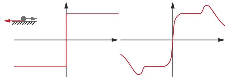
Figure 5: Illustration of the friction model with an example of a point contacting a flat surface in 2D (top left). The exact friction force magnitude (middle) changes abruptly with velocity. Our modified friction force (right) is sufficiently smooth. We further introduce the function $P_{6}$ that attenuates the force magnitude when velocity is sufficiently large, which is essential for our analysis.

6.1 Curvature-bounded Relaxation for Frictional Damping Force

Our analysis of low-level SQP Algorithm 4 relies on the analysis of the vector $\nabla_{\theta_{\star}}\Lambda$ matrix $\nabla_{\theta_{\star}\theta}\Lambda$. The bounds on the singular values of $\nabla_{\theta_{\star}\theta}\Lambda$ require a new analysis, which in turn relies on the specific form of $D(\theta_{i},\theta_{\gamma(i)})$. We present an analysis for the Coulomb’s frictional damping force between a pair of points. Other force models can be analyzed in a similar fashion. We introduce a constant matrix $A\in\mathbb{R}^{3\times\mathcal{C}}$ such that $A\theta_{i}$ is the vector between two points and the distance constraint reads $h_{j}^{i}=\|A\theta_{i}\|-\epsilon_{r}$, then the associated normal vector is ${\partial{h_{j}^{i}}}/{\partial{(A\theta_{i})}}\in\mathbb{R}^{3}$. We assume the contact constraint is modeled as in Section 4.3 using the penalty function $P_{4}(h_{j}^{i},L_{2})$. The normal force magnitude can be computed as $\|{\partial{P_{4}}}/{\partial{x}}(h_{j}^{i},L_{2})\|$. By MDP, our damping force can be formulated as:

$$f_{i}^{d}=-\underbrace{\frac{\nu\left[\sqrt{\left\|\frac{\partial{P_{4}}}{\partial{x}}(h_{j}^{i}(\theta_{i}),L_{2})\right\|^{2}+\epsilon_{r}}-\epsilon_{r}\right]}{\sqrt{\|T(\theta_{i})\dot{\theta}_{i}\|^{2}+\epsilon_{r}}}T(\theta_{i})}_{D(\theta_{i},\theta_{\gamma(i)})}\dot{\theta}_{i}$$ (35)

$$T(\theta_{i})\triangleq\begin{cases}I-\frac{\partial{h_{j}^{i}}}{\partial{A\theta_{i}}}\frac{\partial{h_{j}^{i}}}{\partial{A\theta_{i}}}^{T}&h_{j}^{i}\geq 0\\ I&\text{otherwise},\end{cases}$$

where we denote by $\nu$ the frictional coefficient and $T(\theta_{i})$ is the projection matrix into the tangent space, by noting that ${\partial{h_{j}^{i}}}/{\partial{(A\theta_{i})}}$ is the unit normal direction. Clearly, $D(\theta_{i},\theta_{\gamma(i)})$ in this case is positive semi-definite. As usually, we introduce a small positive number $\epsilon_{r}$ to acquire smoothness, which essentially smoothen the force model. A similar formulation of such contact model is adopted in [43].

Unfortunately, the original frictional damping model does not have bounded derivatives, which could lead to unstable numerical computations. Instead, we propose a modified friction model denoted as $f_{i}^{d\star}(\theta_{i},\theta_{\gamma(i)},L_{17})$ that relies on an additional tangent velocity bound $L_{17}$. Our main idea is to limit the magnitude of $\dot{\theta}_{i}$ when its magnitude is larger than a threshold, as illustrated in Figure 5. To this end, we introduce the following limiter function:

$$P_{6}(x,L_{17})=$$

$$\begin{cases}1&x<L_{17}/2\\ -3(L_{17}/x)^{5}+23(L_{17}/x)^{4}-68(L_{17}/x)^{3}+96(L_{17}/x)^{2}-64(L_{17}/x)+17&x<L_{17}\\ L_{17}/x&\text{otherwise}\\ \end{cases},$$

and plug in the upper bounded $\dot{\bar{\theta}}_{i}\triangleq\dot{\theta}_{i}P_{6}(\|\dot{\theta}_{i}\|,L_{17})$ into $f_{i}^{d}$, yielding:

$$f_{i}^{d\star}= -\underbrace{\frac{\nu\left[\sqrt{\left\|\frac{\partial{P_{4}}}{\partial{x}}(h_{j}^{i}(\theta_{i}),L_{2})\right\|^{2}+\epsilon_{r}}-\epsilon_{r}\right]P_{6}(\|\dot{\theta}_{i}\|,L_{17})}{\sqrt{\|T(\theta_{i})\dot{\bar{\theta}}_{i}\|^{2}+\epsilon_{r}}}T(\theta_{i})}_{D(\theta_{i},\theta_{\gamma(i)})}\dot{\theta}_{i}$$ (36)

$$= -\frac{\nu\left[\sqrt{\left\|\frac{\partial{P_{4}}}{\partial{x}}(h_{j}^{i}(\theta_{i}),L_{2})\right\|^{2}+\epsilon_{r}}-\epsilon_{r}\right]}{\sqrt{\|T(\theta_{i})\dot{\bar{\theta}}_{i}\|^{2}+\epsilon_{r}}}T(\theta_{i})\dot{\bar{\theta}}_{i}.$$

As spelled out above, $f_{i}^{d\star}$ still conforms to our definition of damping force (Equation 33). We show some convenient properties for further analysis, which bridges the gap between $f_{i}^{d\star}$ and $f_{i}^{d}$ when $\dot{\theta}_{i}$ is sufficiently small:

Corollary 13

(i) $\dot{\bar{\theta}}_{i}$ is twice differentiable with locally Lipschitz second derivatives; (ii) $\|\dot{\bar{\theta}}_{i}\|\leq L_{17}$; (iii) $\dot{\bar{\theta}}_{i}=\dot{\theta}_{i}$ and $f_{i}^{d}=f_{i}^{d\star}$ when $\|\dot{\theta}_{i}\|\leq L_{17}/2$; (iv) $\|{\partial{\dot{\bar{\theta}}_{i}}}/{\partial{\theta_{i}}}\|\leq L_{18}/\delta_{i}$ and $\|{\partial{\dot{\bar{\theta}}_{i}}}/{\partial{\theta_{\gamma(i)}}}\|\leq L_{18}/\delta_{i}$ for some $L_{18}$ independent of $L_{17}$.

Corollary 13 (i)-(iii) are obvious and we prove (iv). The two cases, ${\partial{\dot{\bar{\theta}}_{i}}}/{\partial{\theta_{i}}}$ and ${\partial{\dot{\bar{\theta}}_{i}}}/{\partial{\theta_{\gamma(i)}}}$ are symmetric and we only prove the former by considering the three cases in $P_{6}$. Case I: If $\|\dot{\theta}_{i}\|<L_{17}/2$, then:

$$\left\|\frac{\partial{\dot{\bar{\theta}}_{i}}}{\partial{\theta_{i}}}\right\|=\left\|\frac{\partial{\dot{\theta}_{i}}}{\partial{\theta_{i}}}\right\|=\frac{1}{\delta_{i}}.$$

Case II: When $L_{17}\leq\|\dot{\theta}_{i}\|$, then:

$$\left\|\frac{\partial{\dot{\bar{\theta}}_{i}}}{\partial{\theta_{i}}}\right\|=L_{17}\left\|\frac{\partial{}}{\partial{\theta_{i}}}\left[\frac{\dot{\theta}_{i}}{\|\dot{\theta}_{i}\|}\right]\right\|=\frac{L_{17}}{\delta_{i}}\left\|\frac{\partial{}}{\partial{\dot{\theta}_{i}}}\left[\frac{\dot{\theta}_{i}}{\|\dot{\theta}_{i}\|}\right]\right\|\leq\frac{1}{\|\dot{\theta}_{i}\|}\frac{L_{17}}{\delta_{i}}\leq\frac{1}{\delta_{i}}.$$

Case III: Otherwise, we have the following estimate:

$$\left\|\frac{\partial{\dot{\bar{\theta}}_{i}}}{\partial{\theta_{i}}}\right\|= \left\|P_{6}(\|\dot{\theta}_{i}\|,L_{17})\frac{\partial{\dot{\theta}_{i}}}{\partial{\theta_{i}}}+\dot{\theta}_{i}\frac{\partial{P_{6}(\|\dot{\theta}_{i}\|,L_{17})}}{\partial{\theta_{i}}}^{T}\right\|$$

$$= \left\|\frac{P_{6}(\|\dot{\theta}_{i}\|,L_{17})}{\delta_{i}}I+\frac{\partial{P_{6}(\|\dot{\theta}_{i}\|,L_{17})}}{\partial{\|\dot{\theta}_{i}\|}}\dot{\theta}_{i}\frac{\partial{\|\dot{\theta}_{i}\|}}{\partial{\theta_{i}}}^{T}\right\|$$

$$\leq \frac{P_{6}(\|\dot{\theta}_{i}\|,L_{17})}{\delta_{i}}+\frac{\|\dot{\theta}_{i}\|}{\delta_{i}}\left|\frac{\partial{P_{6}(\|\dot{\theta}_{i}\|,L_{17})}}{\partial{\|\dot{\theta}_{i}\|}}\right|.$$

TO derive our desired result, we note that, in Case III, $P_{6}(x,L_{17})$ can be written as a polynomial of $L_{17}/x$, denoted as $\text{poly}_{6}(L_{17}/x)$. By the chain rule, its derivative can be written as $\text{poly}_{6}^{\prime}(L_{17}/x)/x$. Plugging these into the above estimate, and we have:

$$\left\|\frac{\partial{\dot{\bar{\theta}}_{i}}}{\partial{\theta_{i}}}\right\|\leq\frac{\text{poly}_{6}(L_{17}/\|\dot{\theta}_{i}\|)}{\delta_{i}}+\frac{\text{poly}_{6}^{\prime}(L_{17}/\|\dot{\theta}_{i}\|)}{\delta_{i}}\leq\frac{1}{\delta_{i}}\underset{x\in[1/2,1]}{\max}(\text{poly}_{6}(x)+\text{poly}_{6}^{\prime}(x)),$$

yielding our desired result. Corollary 13 can be proved by direct verification using a similar argument as Corollary 4. Next, we re-establish an equivalent result to Corollary 1, where we use the following modified definitions of matrices to incorporate our frictional damping:

$$\nabla_{\theta_{\star}}\Lambda\triangleq\left(\begin{array}[]{c}\vdots\\ \frac{\partial{\bar{E}_{\theta_{\gamma^{2}(N)}}}}{\partial{\theta_{\gamma^{2}(N)}}}-f_{i}^{d\star}(\theta_{\gamma^{2}(N)},\theta_{\gamma^{3}(N)},L_{17})\\ \frac{\partial{\bar{E}_{\theta_{\gamma(N)}}}}{\partial{\theta_{\gamma(N)}}}-f_{i}^{d\star}(\theta_{\gamma(N)},\theta_{\gamma^{2}(N)},L_{17})\\ \frac{\partial{\bar{E}_{\theta_{N}}}}{\partial{\theta_{N}}}-f_{i}^{d\star}(\theta_{N},\theta_{\gamma(N)},L_{17})\end{array}\right)\quad\nabla_{\theta_{\star}\theta}\Lambda\triangleq\frac{\partial{\nabla_{\theta_{\star}}\Lambda}}{\partial{\theta}}.$$ (41)

Lemma 17

The derivatives of the modified friction force in Equation 36 (i) are locally Lipschitz continuous and (ii) has $\text{poly}(L_{2})/\delta_{i}$-bounded singular values, i.e.:

$$\sigma_{\max}({\partial{f_{i}^{d\star}}}/{\partial{\theta_{\gamma(i)}}})\leq\text{poly}(L_{2})/\delta_{i}\;\text{and}\;\sigma_{\max}({\partial{f_{i}^{d\star}}}/{\partial{\theta_{i}}})\leq\text{poly}(L_{2})/\delta_{i}.$$

Lemma 17 (i) We consider two cases. Case I: If $h_{j}^{i}<1/(3L_{2})$, then $h_{j}^{i}\leq 1/(3L_{2})$ in a local neighborhood around $\theta_{i}$, so $P_{4}$ along with its derivatives are all zero by its definition. Therefore, $f_{i}^{d\star}$ and its derivatives are all zero and local Lipschitz continuity trivially holds. Case II: If $h_{j}^{i}\geq 1/(3L_{2})$, then we need to analyze the derivatives of $f_{i}^{d\star}$ term by term. We consider the derivatives with respect to $\theta_{\gamma(i)}$ first:

$$\frac{\partial{f_{i}^{d\star}}}{\partial{\theta_{\gamma(i)}}}=-\nu\left[\sqrt{\left\|\frac{\partial{P_{4}}}{\partial{x}}(h_{j}^{i}(\theta_{i}),L_{2})\right\|^{2}+\epsilon_{r}}-\epsilon_{r}\right]\underbrace{\frac{\partial{}}{\partial{\theta_{\gamma(i)}}}\left[\frac{T(\theta_{i})\dot{\bar{\theta}}_{i}}{\sqrt{\|T(\theta_{i})\dot{\bar{\theta}}_{i}\|^{2}+\epsilon_{r}}}\right]}_{\text{ii}}.$$

Since ${\partial{P_{4}}}/{\partial{x}}$ is differentiable by definition, $h_{j}^{i}$ and $T(\theta_{i})$ are differentiable by assumptions in Corollary 4, ${\partial{f_{i}^{d\star}}}/{\partial{\theta_{\gamma(i)}}}$ is differentiable and local Lipschitz continuity holds. Next, we consider the derivatives with respect to $\theta_{i}$:

$$\frac{\partial{f_{i}^{d\star}}}{\partial{\theta_{i}}}= -\nu\underbrace{\left[\sqrt{\left\|\frac{\partial{P_{4}}}{\partial{x}}(h_{j}^{i}(\theta_{i}),L_{2})\right\|^{2}+\epsilon_{r}}-\epsilon_{r}\right]}_{\text{i}}\underbrace{\frac{\partial{}}{\partial{\theta_{i}}}\left[\frac{T(\theta_{i})\dot{\bar{\theta}}_{i}}{\sqrt{\|T(\theta_{i})\dot{\bar{\theta}}_{i}\|^{2}+\epsilon_{r}}}\right]}_{\text{ii'}}+$$

$$\underbrace{\frac{\nu\frac{\partial{P_{4}}}{\partial{x}}(h_{j}^{i}(\theta_{i}),L_{2})}{\sqrt{\left\|\frac{\partial{P_{4}}}{\partial{x}}(h_{j}^{i}(\theta_{i}),L_{2})\right\|^{2}+\epsilon_{r}}}}_{\text{iii}}\underbrace{\frac{\partial^{2}{P_{4}}}{\partial{x}^{2}}(h_{j}^{i}(\theta_{i}),L_{2})}_{\text{iv}}\underbrace{\frac{T(\theta_{i})\dot{\bar{\theta}}_{i}}{\sqrt{\|T(\theta_{i})\dot{\bar{\theta}}_{i}\|^{2}+\epsilon_{r}}}\frac{\partial{h_{j}^{i}}}{\partial{\theta_{i}}}^{T}}_{\text{v}},$$

where there are altogether five terms. Term (i), (ii), (iii), (v) are differentiable by definition of $P_{4}$, assumptions in Corollary 4. Term (iv) is locally Lipschitz continuous by definition of $P_{4}$. Put together, we have ${\partial{f_{i}^{d\star}}}/{\partial{\theta_{\gamma(i)}}}$ is locally Lipschitz continuous.

(ii) We again consider two cases. Case I: If $h_{j}^{i}<1/(3L_{2})$, then derivatives of $f_{i}^{d\star}$ and thus its singular values are all zero, so we focus on case II where $h_{j}^{i}\geq 1/(3L_{2})$. We consider the derivatives with respect to $\theta_{\gamma(i)}$ first:

$$\sigma_{\max}({\partial{f_{i}^{d\star}}}/{\partial{\theta_{\gamma(i)}}})\leq\nu\left\|\frac{\partial{P_{4}}}{\partial{x}}(h_{j}^{i}(\theta_{i}),L_{2})\right\|\sigma_{\max}(ii)$$

$$\sigma_{\max}(ii)\leq\frac{1}{\sqrt{\|T(\theta_{i})\dot{\bar{\theta}}_{i}\|^{2}+\epsilon_{r}}}\left\|I-\frac{T(\theta_{i})\dot{\bar{\theta}}_{i}\dot{\bar{\theta}}_{i}^{T}T(\theta_{i})^{T}}{\|T(\theta_{i})\dot{\bar{\theta}}_{i}\|^{2}+\epsilon_{r}}\right\|\left\|\frac{\partial{T(\theta_{i})\dot{\bar{\theta}}_{i}}}{\partial{\theta_{\gamma(i)}}}\right\|$$

$$\leq \frac{1}{\delta_{i}\sqrt{\|T(\theta_{i})\dot{\bar{\theta}}_{i}\|^{2}+\epsilon_{r}}}\left\|I-\frac{T(\theta_{i})\dot{\bar{\theta}}_{i}\dot{\bar{\theta}}_{i}^{T}T(\theta_{i})^{T}}{\|T(\theta_{i})\dot{\bar{\theta}}_{i}\|^{2}+\epsilon_{r}}\right\|\|T(\theta_{i})\|L_{18}\leq\frac{1}{\delta_{i}\sqrt{\epsilon_{r}}},$$

where we used the fact that $\sigma_{\max}(T(\theta_{i}))\leq 1$. Since $\|{\partial{P_{4}}}/{\partial{x}}\|$ is $\text{poly}(L_{2})$ upper bounded by definition, $\sigma_{\max}({\partial{f_{i}^{d\star}}}/{\partial{\theta_{\gamma(i)}}})$ is $\text{poly}(L_{2})/\delta_{i}$ upper bounded as desired. Next, we consider the derivatives with respect to $\theta_{i}$:

$$\sigma_{\max}({\partial{f_{i}^{d\star}}}/{\partial{\theta_{i}}})\leq \underbrace{\nu\left\|\frac{\partial{P_{4}}}{\partial{x}}(h_{j}^{i}(\theta_{i}),L_{2})\right\|}_{i}\sigma_{\max}(ii^{\prime})+\underbrace{\nu}_{iii}\underbrace{\left\|\frac{\partial^{2}{P_{4}}}{\partial{x}^{2}}(h_{j}^{i}(\theta_{i}),L_{2})\right\|}_{iv}\sigma_{\max}(v)$$

$$\leq \nu\text{poly}(L_{2})(\sigma_{\max}(ii^{\prime})+\sigma_{\max}(v)),$$

where we need to further bound term (ii’) and (v). For term (ii’), we use a similar technique as term (ii) and the bound on $\dot{\bar{\theta}}_{i}$ to have:

$$\sigma_{\max}(ii^{\prime})$$

$$\leq \frac{1}{\sqrt{\|T(\theta_{i})\dot{\bar{\theta}}_{i}\|^{2}+\epsilon_{r}}}\left\|I-\frac{T(\theta_{i})\dot{\bar{\theta}}_{i}\dot{\bar{\theta}}_{i}^{T}T(\theta_{i})^{T}}{\|T(\theta_{i})\dot{\bar{\theta}}_{i}\|^{2}+\epsilon_{r}}\right\|\left\|\frac{\partial{T(\theta_{i})\dot{\bar{\theta}}_{i}}}{\partial{\theta_{i}}}\right\|$$

$$\leq \frac{1}{\sqrt{\|T(\theta_{i})\dot{\bar{\theta}}_{i}\|^{2}+\epsilon_{r}}}\left\|\frac{\partial{T(\theta_{i})\dot{\bar{\theta}}_{i}}}{\partial{\theta_{i}}}\right\|$$

$$\leq \frac{1}{\sqrt{\|T(\theta_{i})\dot{\bar{\theta}}_{i}\|^{2}+\epsilon_{r}}}\left[\frac{L_{18}}{\delta_{i}}\left\|T(\theta_{i})\right\|+\left\|\frac{\partial{T(\theta_{i})}}{\partial{\theta_{i}}}:\dot{\bar{\theta}}_{i}\right\|\right]$$

$$= \frac{1}{\sqrt{\|T(\theta_{i})\dot{\bar{\theta}}_{i}\|^{2}+\epsilon_{r}}}\left[\frac{L_{18}}{\delta_{i}}\left\|T(\theta_{i})\right\|+\left\|\frac{\partial{h_{j}^{i}}}{\partial{A\theta_{i}}}^{T}\dot{\bar{\theta}}_{i}\frac{\partial{}}{\partial{\theta_{i}}}\frac{\partial{h_{j}^{i}}}{\partial{A\theta_{i}}}+\frac{\partial{h_{j}^{i}}}{\partial{A\theta_{i}}}\dot{\bar{\theta}}_{i}^{T}\frac{\partial{}}{\partial{\theta_{i}}}\frac{\partial{h_{j}^{i}}}{\partial{A\theta_{i}}}\right\|\right]$$

$$\leq \frac{1}{\sqrt{\epsilon_{r}}}\left[\frac{L_{18}}{\delta_{i}}+2L_{17}\sup_{h_{j}^{i}\geq 1/(3L_{2})}\left\|\frac{\partial{}}{\partial{\theta_{i}}}\frac{\partial{h_{j}^{i}}}{\partial{A\theta_{i}}}\right\|\right],$$

where the last $\sup$ must be bounded. Indeed, it corresponds the maximal geometric curvature of the two spheres in collision. For term (v), we have:

$$\sigma_{\max}(v)=\left\|\frac{T(\theta_{i})\dot{\bar{\theta}}_{i}}{\sqrt{\|T(\theta_{i})\dot{\bar{\theta}}_{i}\|^{2}+\epsilon_{r}}}\frac{\partial{h_{j}^{i}}}{\partial{\theta_{i}}}^{T}\right\|$$

$$\leq \left\|\frac{T(\theta_{i})\dot{\bar{\theta}}_{i}}{\sqrt{\|T(\theta_{i})\dot{\bar{\theta}}_{i}\|^{2}+\epsilon_{r}}}\right\|\left\|\frac{\partial{h_{j}^{i}}}{\partial{\theta_{i}}}\right\|\leq\sup_{h_{j}^{i}\geq 1/(3L_{2})}\left\|\frac{\partial{h_{j}^{i}}}{\partial{\theta_{i}}}\right\|,$$

where we use the assumption in Corollary 4 that the function $h_{j}^{i}$ and its derivatives have bounded norm when $h_{j}^{i}\geq 0$. Combining the above bounds, we have the desired results. We are now ready to prove the main results playing equivalent roles to Corollary 1 and Lemma 3:

Corollary 14

Denoting $L=\text{poly}(L_{2})$ and assuming Equation 41, if $\bar{P}$ is $\text{poly}(L_{2})$-curvature-bounded and $\delta_{i}<2\sigma_{min}(M)/(\sqrt{L^{2}+4\sigma_{min}(M)L}+L)$ for all $i$, then (i) the function $\Lambda_{i}(\theta_{i})\triangleq\|{\partial{E_{i}}}/{\partial{\theta_{i}}}-f_{i}^{d\star}\|^{2}/2$ satisfies the PL condition; (ii) $\sigma_{\min}(\nabla_{\theta_{\star}\theta}\Lambda)$ is bounded away from zero and (iii) the accumulated function $\Lambda(\theta)\triangleq\sum_{i}\Lambda_{i}$ also satisfies the PL condition.

(ii) the accumulated function $\Lambda(\theta)\triangleq\sum_{i}\Lambda_{i}$ also satisfies the PL condition.

Corollary 14 (i) Using Lemma 17, we have following estimate under the above choice of $\delta_{i}$:

$$\sigma_{\min}\left(\nabla_{\theta_{\star}\theta}\Lambda_{ii}\right)\geq\frac{\sigma_{\min}(M)}{\delta_{i}^{2}}-L-\frac{L}{\delta_{i}}>0.$$

The PL condition immediately satisfies by noting that:

$$\left\|\frac{\partial{\Lambda_{i}}}{\partial{\theta_{i}}}\right\|^{2}=\left\|\nabla_{\theta_{\star}\theta}\Lambda_{ii}\nabla_{\theta_{\star}}\Lambda_{i}\right\|^{2}\geq\left[\frac{\sigma_{\min}(M)}{\delta_{i}^{2}}-L-\frac{L}{\delta_{i}}\right]^{2}\left\|\nabla_{\theta_{\star}}\Lambda_{i}\right\|^{2}.$$

(ii) By our updated definition of matrices in Equation 41, we can still use the estimate that:

$$\left\|\frac{\partial{\Lambda}}{\partial{\theta}}\right\|^{2}\geq 2\sigma_{\min}(\nabla_{\theta_{\star}\theta}\Lambda)^{2}\Lambda,$$

and the bound in Equation LABEL:eq:SigmaMinBound. However, the bound on $\alpha,\beta$ needs to be updated as:

$$\beta\geq \underset{i}{\min}\left[\frac{\sigma_{\min}(M)}{\delta_{i}^{2}}-L-\frac{L}{\delta_{i}}\right]>0$$

$$\alpha\leq \left[\underset{i}{\max}\left[\left[\frac{1}{\delta_{i}^{2}},\frac{1}{\delta_{i}\delta_{\gamma(i)}},\frac{1+\delta_{i}/\delta_{\gamma(i)}}{\delta_{i}^{2}}\right]\sigma_{\max}(M)+L+\frac{L}{\delta_{i}}\right]\right]/$$

$${\underset{i}{\min}\left[\frac{\sigma_{\min}(M)}{\delta_{i}^{2}}-L-\frac{L}{\delta_{i}}\right]},$$

and all is proved.

Lemma 18

Assuming Equation 41, Assumption 3.2, and Assumption 3.3, we have that (i) $\sigma_{\max}(\nabla_{\theta_{\star}\theta}\Lambda)$ is upper bounded; and (ii) under Assumption 3.3, $\sigma_{\max}(\nabla_{\theta_{\star}u}\Lambda)$ is upper bounded.

Lemma 18 (i) We propose a very pessimistic estimate using Lemma 17:

$$\sigma_{\max}(\nabla_{\theta_{\star}\theta}\Lambda)=\|\nabla_{\theta_{\star}\theta}\Lambda\|$$

$$\leq \sum_{i}\left[\left\|\nabla_{\theta_{\star}\theta}\Lambda_{i\gamma^{2}(i)}\right\|+\left\|\nabla_{\theta_{\star}\theta}\Lambda_{i\gamma(i)}\right\|+\left\|\nabla_{\theta_{\star}}\Lambda_{i}\right\|\right]$$

$$\leq |\mathcal{D}|\left[\underset{i}{\max}\left[\left[\frac{1}{\delta_{i}^{2}}+\frac{1}{\delta_{i}\delta_{\gamma(i)}}+\frac{1+\delta_{i}/\delta_{\gamma(i)}}{\delta_{i}^{2}}\right]\sigma_{\max}(M)+L+\frac{L}{\delta_{i}}\right]\right],$$

where we denote $L=\text{poly}(L_{2})$. (ii) holds by the same argument as in Lemma 3. With Equation LABEL:eq:Definition, Corollary 1 and Lemma 3 replaced by Equation 41, Corollary 14 and Lemma 18, respectively, all the results in Section 3.2 still hold by the same argument.

6.2 Hamiltonian Upper Bound

Our entire Section 5.1 is built on top of the one-step upper bound of Hamiltonian change provided by Lemma 12. Since damping forces only reduce the energy, this one-step upper bound should hold as before and we formalize this result below:

Lemma 19

For damped dynamic system Equation 34, if $\bar{P}$ is $L$-weakly convex, and $\theta_{i}$ is an $\epsilon$-critical point of Equation LABEL:eq:EOMApprox satisfying $2\Lambda_{i}\leq\epsilon^{2}$, then we have:

$$H_{i}(\theta_{i},\theta_{\gamma(i)},u_{\iota(i)},L_{2})-H_{\gamma(i)}(\theta_{\gamma(i)},\theta_{\gamma^{2}(i)},u_{\iota(i)},L_{2})$$

$$\leq \frac{L\delta_{i}^{2}+\delta_{i}}{2\sigma_{\min}(M)}\left\|\frac{\theta_{i}-\theta_{\gamma(i)}}{\delta_{i}}\right\|_{M}^{2}+\frac{\delta_{i}\epsilon^{2}}{2}.$$

Lemma 19 The local solution of Equation LABEL:eq:EOMApprox implies:

$$\frac{\theta_{i}-\theta_{\gamma(i)}}{\delta_{i}}-\frac{\theta_{\gamma(i)}-\theta_{\gamma^{2}(i)}}{\delta_{\gamma(i)}}+M^{-1}D(\theta_{i},\theta_{\gamma(i)})(\theta_{i}-\theta_{\gamma(i)})+\delta_{i}M^{-1}\frac{\partial{\bar{P}}}{\partial{\theta_{i}}}(\theta_{i},u_{\iota(i)},L_{2})=r_{i}$$

$$\;\text{and}\;\left\|\frac{Mr_{i}}{\delta_{i}}\right\|\leq\epsilon.$$

Plugging this into the definition of Hamiltonian and we have:

$$H_{i}(\theta_{i},\theta_{\gamma(i)},u_{\iota(i)},L_{2})-H_{\gamma(i)}(\theta_{\gamma(i)},\theta_{\gamma^{2}(i)},u_{\iota(i)},L_{2})$$

$$= \frac{1}{2}\left\|\frac{\theta_{i}-\theta_{\gamma(i)}}{\delta_{i}}\right\|_{M}^{2}-\frac{1}{2}\left\|\frac{\theta_{i}-\theta_{\gamma(i)}}{\delta_{i}}+M^{-1}D(\theta_{i},\theta_{\gamma(i)})(\theta_{i}-\theta_{\gamma(i)})+\delta_{i}M^{-1}\frac{\partial{\bar{P}}}{\partial{\theta_{i}}}-r_{i}\right\|_{M}^{2}+$$

$$\bar{P}(\theta_{i},u_{\iota(i)},L_{2})-\bar{P}(\theta_{\gamma(i)},u_{\iota(i)},L_{2})$$

$$= \bar{P}(\theta_{i},u_{\iota(i)},L_{2})-\bar{P}(\theta_{\gamma(i)},u_{\iota(i)},L_{2})-$$

$$\frac{1}{2}\left\|M^{-1}D(\theta_{i},\theta_{\gamma(i)})(\theta_{i}-\theta_{\gamma(i)})+\delta_{i}M^{-1}\frac{\partial{\bar{P}}}{\partial{\theta_{i}}}-r_{i}\right\|_{M}^{2}-$$

$$(\theta_{i}-\theta_{\gamma(i)})^{T}\frac{\partial{\bar{P}}}{\partial{\theta_{i}}}+(\theta_{i}-\theta_{\gamma(i)})^{T}\frac{Mr_{i}}{\delta_{i}}-\|\theta_{i}-\theta_{\gamma(i)}\|^{2}_{D(\theta_{i},\theta_{\gamma(i)})/\delta_{i}}$$

$$\leq \frac{L}{2}\|\theta_{i}-\theta_{\gamma(i)}\|^{2}-(\theta_{i}-\theta_{\gamma(i)})^{T}\frac{Mr_{i}}{\delta_{i}}$$

$$\leq \frac{L\delta_{i}^{2}}{2}\left\|\frac{\theta_{i}-\theta_{\gamma(i)}}{\delta_{i}}\right\|^{2}+\frac{\delta_{i}}{2}\left\|\frac{\theta_{i}-\theta_{\gamma(i)}}{\delta_{i}}\right\|^{2}+\frac{\delta_{i}}{2}\left\|\frac{Mr_{i}}{\delta_{i}}\right\|^{2}$$

$$\leq \frac{L\delta_{i}^{2}+\delta_{i}}{2\sigma_{\min}(M)}\left\|\frac{\theta_{i}-\theta_{\gamma(i)}}{\delta_{i}}\right\|_{M}^{2}+\frac{\delta_{i}\epsilon^{2}}{2},$$

where we have use the $L$-weak convexity and the fact that $D(\theta_{i},\theta_{\gamma(i)})$ is positive semi-definite in the first inequality. Replacing Lemma 12 by Lemma 19, it can be verified that Lemma 13 and Lemma 14 hold by the identical arguments, but we need to following result to replace Lemma 15:

Definition 6.1

We say a solution $\theta_{i}$ satisfies the $\epsilon$-perturbed KKT condition of the equation of motion (Equation 34) if:

$$\text{KKT-EOM}_{i}^{\epsilon}:\begin{cases}\left\|M\ddot{\theta}_{i}-f-f_{i}^{d}+g+\frac{\partial{b}}{\partial{\theta_{i}}}+\sum_{j}\mu_{j}^{e}\frac{\partial{h_{j}^{e}}}{\partial{\theta_{i}}}+\sum_{j}\mu_{j}^{i}\frac{\partial{h_{j}^{i}}}{\partial{\theta_{i}}}\right\|\leq\epsilon\\ |h_{j}^{e}(\theta_{i})|\leq\epsilon\\ h_{j}^{i}(\theta_{i})\geq 0\\ \mu_{j}^{i}\leq 0\\ \mu_{j}^{i}\underset{}{\max}(h_{j}^{i}-\epsilon,0)=0\\ \end{cases},$$ (42)

for some $\mu_{j}^{e}$ and $\mu_{j}^{i}$, and we call such $\theta_{i}$ the $\text{KKT-EOM}_{i}^{\epsilon}$ solution.

Lemma 20

For damped dynamic system Equation 34, under the same assumption as Lemma 14 and for a chosen $\epsilon$, if we further let $L_{2}>\max(1/\epsilon,L_{14}^{i})$, $L_{17}=2\sqrt{2L_{14}^{N}/\sigma_{\min}(M)}$, and $2\Lambda_{i}\leq\epsilon^{2}$, then $\theta_{i}$ is the $\text{KKT-EOM}_{i}^{\epsilon}$ solution of Equation 1.

Lemma 20 The last four $\text{KKT-EOM}_{i}^{\epsilon}$ conditions satisfy using exactly the same argument as in Lemma 15. For the first condition, we expand the condition that $2\Lambda_{i}\leq\epsilon^{2}$:

$$2\Lambda_{i}=\left\|M\ddot{\theta}_{i}-f-f_{i}^{d\star}(\theta_{i},\theta_{\gamma(i)},L_{17})+g+\frac{\partial{b}}{\partial{\theta_{i}}}+\sum_{j}\mu_{j}^{e}\frac{\partial{h_{j}^{e}}}{\partial{\theta_{i}}}+\sum_{j}\mu_{j}^{i}\frac{\partial{h_{j}^{i}}}{\partial{\theta_{i}}}\right\|^{2}\leq\epsilon^{2},$$

where the only difference from the first condition in $\text{KKT-EOM}_{i}^{\epsilon}$ lies in the difference between $f_{i}^{d}$ and $f_{i}^{d\star}$. By Lemma 14 and our choice of $L_{17}$, we have the following bound on $\dot{\theta}_{i}$:

$$\frac{\sigma_{\min}(M)}{2}\|\dot{\theta}_{i}\|^{2}\leq\frac{1}{2}\|\dot{\theta}_{i}\|_{M}^{2}\leq L_{14}^{i}$$

$$\Rightarrow \|\dot{\theta}_{i}\|\leq\sqrt{2L_{14}^{i}/\sigma_{\min}(M)}\leq\sqrt{2L_{14}^{N}/\sigma_{\min}(M)}=L_{17}/2,$$

in which case we know that $f_{i}^{d}=f_{i}^{d\star}$ by Corollary 13 (iii), so all is proved. All the results after Lemma 15 follow exactly the same argument, if we (i) assume the choice of $L_{17}$ as in Lemma 20 and (ii) replace the bound $\delta_{i}<\sqrt{\sigma_{\min}(M)/L}$ from Lemma 2 by the bound $\delta_{i}<2\sigma_{min}(M)/(\sqrt{L^{2}+4\sigma_{min}(M)L}+L)$ from Corollary 14.

7 Conclusion

We propose a theoretical framework for solving TO under general dynamic system constraints. Our dynamic system can be arbitrarily stiff, i.e., undergoing rapidly changing forces or general (in)equality constraints. These problems find a wide spectrum of applications in robotic research and practice, including automatic gait discovery and whole-body motion control. Unlike existing black-box TO algorithms, where the underlying NLP solver is not allowed to modify the problem setting, we propose a white-box TO algorithm. Our algorithm has the underlying NLP solver informed of the properties of the dynamic system and the discretization scheme. We show that if the curvature of the potential energy can be bounded and the timestep size can be adaptively subdivided, a white-box TO algorithm based on low-level SQP solver can converge globally to a stationary solution of the TO problem in a numerically stable manner. To the best of our knowledge, these guarantees are unavailable in prior black-box TO solvers. As our main technique of analysis, we first show that the curvature boundedness of the potential energy ensures the stability and global convergence of the underlying SQP solver (Section 3.2). Further, we show that the Hamiltonian operator depicting the total energy is upper bounded on convergence, leading to accurate time integration of the underlying dynamic system (Section 5.1). Finally, we show that our assumptions hold for various dynamic systems used in practical robotic research problems (Section 4 and Section 5.3).

Our technique is a first step towards theoretically guaranteed TO solvers, leading to several avenues of future research. First, our technique only shows that the TO solver converges but we do not analyze the algorithmic complexity. Providing a complexity bound is the first step towards the design of more efficient TO solvers and gauging the efficacy of different algorithms. Indeed, we make little efforts in designing efficient TO solvers, and we believe several techniques can be used to improve the efficacy of our basic algorithm. For example, we could use different $L_{2}$ constants for different potential energy terms, in order to reduce the unnecessary stiffness of the dynamic system. But these advanced techniques would complicate our convergence analysis. Finally, we are interested in extending our technique to incorporate more general dynamic system models and time discretization schemes.

References

• [1] Aceituno-Cabezas, B., Rodriguez, A.: A Global Quasi-Dynamic Model for Contact-Trajectory Optimization in Manipulation. In: Proceedings of Robotics: Science and Systems. Corvalis, Oregon, USA (July 2020). https://doi.org/10.15607/RSS.2020.XVI.047
• [2] Alizadeh, F., Goldfarb, D.: Second-order cone programming. Mathematical programming 95(1), 3–51 (2003)
• [3] Amenta, N., Choi, S., Kolluri, R.K.: The power crust, unions of balls, and the medial axis transform. Computational Geometry 19(2-3), 127–153 (2001)
• [4] Anitescu, M.: On solving mathematical programs with complementarity constraints as nonlinear programs. Preprint ANL/MCS-P864-1200, Argonne National Laboratory, Argonne, IL 3 (2000)
• [5] Ashi, H.: Numerical methods for stiff systems. Ph.D. thesis, University of Nottingham (2008)
• [6] Aydinoglu, A., Wei, A., Huang, W.C., Posa, M.: Consensus complementarity control for multi-contact mpc. arXiv preprint arXiv:2304.11259 (2023)
• [7] Bertsekas, D.P.: Nonlinear programming. Journal of the Operational Research Society 48(3), 334–334 (1997)
• [8] Biegler, L.T., Zavala, V.M.: Large-scale nonlinear programming using ipopt: An integrating framework for enterprise-wide dynamic optimization. Computers & Chemical Engineering 33(3), 575–582 (2009)
• [9] Bouzidi, R., Le Van, A.: Numerical solution of hyperelastic membranes by energy minimization. Computers and structures 82(23-26), 1961–1969 (2004)
• [10] Brogliato, B., Brogliato, B.: Nonsmooth mechanics, vol. 3. Springer (1999)
• [11] Brüdigam, J., Manchester, Z.: Linear-quadratic optimal control in maximal coordinates. In: 2021 IEEE International Conference on Robotics and Automation (ICRA). pp. 9775–9781. IEEE (2021)
• [12] Brüdigam, J., Schuck, M., Capone, A., Sosnowski, S., Hirche, S.: Structure-preserving learning using gaussian processes and variational integrators. In: Learning for Dynamics and Control Conference. pp. 1150–1162. PMLR (2022)
• [13] Chatzinikolaidis, I., You, Y., Li, Z.: Contact-implicit trajectory optimization using an analytically solvable contact model for locomotion on variable ground. IEEE Robotics and Automation Letters 5(4), 6357–6364 (2020)
• [14] Dai, H., Izatt, G., Tedrake, R.: Global inverse kinematics via mixed-integer convex optimization. The International Journal of Robotics Research 38(12-13), 1420–1441 (2019)
• [15] Escande, A., Miossec, S., Benallegue, M., Kheddar, A.: A strictly convex hull for computing proximity distances with continuous gradients. IEEE Transactions on Robotics 30(3), 666–678 (2014). https://doi.org/10.1109/TRO.2013.2296332
• [16] Gill, P.E., Murray, W., Saunders, M.A.: Snopt: An sqp algorithm for large-scale constrained optimization. SIAM review 47(1), 99–131 (2005)
• [17] Grinspun, E., Hirani, A.N., Desbrun, M., Schröder, P.: Discrete shells. In: Proceedings of the 2003 ACM SIGGRAPH/Eurographics symposium on Computer animation. pp. 62–67. Citeseer (2003)
• [18] Harmon, D., Vouga, E., Smith, B., Tamstorf, R., Grinspun, E.: Asynchronous contact mechanics. Commun. ACM 55(4), 102–109 (apr 2012). https://doi.org/10.1145/2133806.2133828, https://doi.org/10.1145/2133806.2133828
• [19] Higham, N.J.: A survey of condition number estimation for triangular matrices. Siam Review 29(4), 575–596 (1987)
• [20] Horn, R.A., Johnson, C.R.: Matrix analysis. Cambridge university press (2012)
• [21] Kane, C., Marsden, J.E., Ortiz, M., West, M.: Variational integrators and the newmark algorithm for conservative and dissipative mechanical systems. International Journal for numerical methods in engineering 49(10), 1295–1325 (2000)
• [22] Karimi, H., Nutini, J., Schmidt, M.: Linear convergence of gradient and proximal-gradient methods under the polyak-łojasiewicz condition. In: Machine Learning and Knowledge Discovery in Databases: European Conference, ECML PKDD 2016, Riva del Garda, Italy, September 19-23, 2016, Proceedings, Part I 16. pp. 795–811. Springer (2016)
• [23] Kouvaritakis, B., Cannon, M.: Model predictive control. Switzerland: Springer International Publishing 38 (2016)
• [24] Landry, B., Lorenzetti, J., Manchester, Z., Pavone, M.: Bilevel optimization for planning through contact: A semidirect method. In: The International Symposium of Robotics Research. pp. 789–804. Springer (2019)
• [25] Manchester, Z., Doshi, N., Wood, R.J., Kuindersma, S.: Contact-implicit trajectory optimization using variational integrators. The International Journal of Robotics Research 38(12-13), 1463–1476 (2019)
• [26] Manchester, Z., Kuindersma, S.: Variational contact-implicit trajectory optimization. In: Robotics Research: The 18th International Symposium ISRR. pp. 985–1000. Springer (2020)
• [27] Na, S.: Global convergence of online optimization for nonlinear model predictive control. Advances in Neural Information Processing Systems 34, 12441–12453 (2021)
• [28] Na, S., Anitescu, M.: Superconvergence of online optimization for model predictive control. IEEE Transactions on Automatic Control 68(3), 1383–1398 (2022)
• [29] Nesterov, Y., et al.: Lectures on convex optimization, vol. 137. Springer (2018)
• [30] Ogden, R.W.: Non-linear elastic deformations. Courier Corporation (1997)
• [31] Osher, S., Fedkiw, R., Piechor, K.: Level set methods and dynamic implicit surfaces. Appl. Mech. Rev. 57(3), B15–B15 (2004)
• [32] Pang, T., Suh, H.T., Yang, L., Tedrake, R.: Global planning for contact-rich manipulation via local smoothing of quasi-dynamic contact models. IEEE Transactions on Robotics (2023)
• [33] Posa, M., Cantu, C., Tedrake, R.: A direct method for trajectory optimization of rigid bodies through contact. The International Journal of Robotics Research 33(1), 69–81 (2014)
• [34] Qian, S., Zi, B., Shang, W.W., Xu, Q.S.: A review on cable-driven parallel robots. Chinese Journal of Mechanical Engineering 31(1), 1–11 (2018)
• [35] Rayleigh, J.W.S.B.: The theory of sound, vol. 2. Macmillan (1896)
• [36] Schulman, J., Duan, Y., Ho, J., Lee, A., Awwal, I., Bradlow, H., Pan, J., Patil, S., Goldberg, K., Abbeel, P.: Motion planning with sequential convex optimization and convex collision checking. The International Journal of Robotics Research 33(9), 1251–1270 (2014)
• [37] Solodov, M.V.: Global convergence of an sqp method without boundedness assumptions on any of the iterative sequences. Mathematical programming 118(1), 1–12 (2009)
• [38] Stella, L., Themelis, A., Sopasakis, P., Patrinos, P.: A simple and efficient algorithm for nonlinear model predictive control. In: 2017 IEEE 56th Annual Conference on Decision and Control (CDC). pp. 1939–1944. IEEE (2017)
• [39] Stewart, D.E., Trinkle, J.C.: An implicit time-stepping scheme for rigid body dynamics with inelastic collisions and coulomb friction. International Journal for Numerical Methods in Engineering 39(15), 2673–2691 (1996)
• [40] Suh, H.J., Simchowitz, M., Zhang, K., Tedrake, R.: Do differentiable simulators give better policy gradients? In: International Conference on Machine Learning. pp. 20668–20696. PMLR (2022)
• [41] Tan, J., Liu, K., Turk, G.: Stable proportional-derivative controllers. IEEE Computer Graphics and Applications 31(4), 34–44 (2011)
• [42] Tassa, Y., Todorov, E.: Stochastic complementarity for local control of discontinuous dynamics. In: Proceedings of Robotics: Science and Systems. Zaragoza, Spain (June 2010). https://doi.org/10.15607/RSS.2010.VI.022
• [43] Tassa, Y., Erez, T., Todorov, E.: Synthesis and stabilization of complex behaviors through online trajectory optimization. In: 2012 IEEE/RSJ International Conference on Intelligent Robots and Systems. pp. 4906–4913. IEEE (2012)
• [44] Theodorou, E., Buchli, J., Schaal, S.: A generalized path integral control approach to reinforcement learning. The Journal of Machine Learning Research 11, 3137–3181 (2010)
• [45] Todorov, E.: A convex, smooth and invertible contact model for trajectory optimization. In: 2011 IEEE International Conference on Robotics and Automation. pp. 1071–1076. IEEE (2011)
• [46] Todorov, E., Erez, T., Tassa, Y.: Mujoco: A physics engine for model-based control. In: 2012 IEEE/RSJ international conference on intelligent robots and systems. pp. 5026–5033. IEEE (2012)
• [47] Wang, Y., Boyd, S.: Fast model predictive control using online optimization. IEEE Transactions on control systems technology 18(2), 267–278 (2009)
• [48] Winkler, A.W., Bellicoso, C.D., Hutter, M., Buchli, J.: Gait and trajectory optimization for legged systems through phase-based end-effector parameterization. IEEE Robotics and Automation Letters 3(3), 1560–1567 (2018)
• [49] Xie, Z., Liu, C.K., Hauser, K.: Differential dynamic programming with nonlinear constraints. In: 2017 IEEE International Conference on Robotics and Automation (ICRA). pp. 695–702. IEEE (2017)
• [50] Yamane, K., Nakamura, Y.: Stable penalty-based model of frictional contacts. In: Proceedings 2006 IEEE International Conference on Robotics and Automation, 2006. ICRA 2006. pp. 1904–1909 (2006). https://doi.org/10.1109/ROBOT.2006.1641984
• [51] Zhang, D., Liang, C., Gao, X., Wu, K., Pan, Z.: Provably robust semi-infinite program under collision constraints via subdivision. arXiv preprint arXiv:2302.01135 (2023)
• [52] Zhou, Z., Zhao, Y.: Accelerated admm based trajectory optimization for legged locomotion with coupled rigid body dynamics. In: 2020 American Control Conference (ACC). pp. 5082–5089. IEEE (2020)