From Latent to Lucid: Transforming Knowledge Graph Embeddings into Interpretable Structures

Abstract

This paper introduces a post-hoc explainable AI method tailored for Knowledge Graph Embedding models. These models are essential to Knowledge Graph Completion yet criticized for their opaque, black-box nature. Despite their significant success in capturing the semantics of knowledge graphs through high-dimensional latent representations, their inherent complexity poses substantial challenges to explainability. Unlike existing methods, our approach directly decodes the latent representations encoded by Knowledge Graph Embedding models, leveraging the principle that similar embeddings reflect similar behaviors within the Knowledge Graph. By identifying distinct structures within the subgraph neighborhoods of similarly embedded entities, our method identifies the statistical regularities on which the models rely and translates these insights into human-understandable symbolic rules and facts. This bridges the gap between the abstract representations of Knowledge Graph Embedding models and their predictive outputs, offering clear, interpretable insights. Key contributions include a novel post-hoc explainable AI method for Knowledge Graph Embedding models that provides immediate, faithful explanations without retraining, facilitating real-time application even on large-scale knowledge graphs. The method’s flexibility enables the generation of rule-based, instance-based, and analogy-based explanations, meeting diverse user needs. Extensive evaluations show our approach’s effectiveness in delivering faithful and well-localized explanations, enhancing the transparency and trustworthiness of Knowledge Graph Embedding models.

1 Introduction

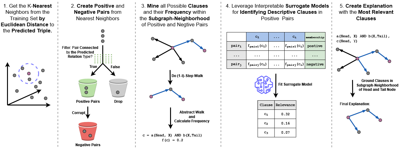
Figure 1: KGExplainer generates post-hoc explanations of KGE models in five steps. The five steps are discussed in detail in Section 3.

Knowledge Graphs (KG), despite their vast potential for structuring and leveraging information, are notoriously incomplete (?; ?). To mitigate this issue, link prediction has emerged as a technique for uncovering previously unknown links within these graphs (?). Knowledge Graph Embedding (KGE) models have become the de facto standard due to their ability to capture the complex relationships and semantics embedded within the graph structure through high-dimensional latent representations (?). However, despite their effectiveness, these models are criticized for their black-box nature (?), which obscures the underlying mechanisms and rationales behind their predictions (?), posing challenges for explainability in critical applications (?; ?).

Explainable Artificial Intelligence (XAI) has made significant progress in demystifying the opaque decision-making processes of complex black-box models (?). Despite the development of explainable methods such as LIME (?), SHAP (?), Layer-wise Relevance Propagation (?), and Integrated Gradients (?), applying these methods to KGE models presents a non-trivial challenge. These methods traditionally work by attributing parts of the input as relevant or not to the model’s output. However, embedding-based link prediction operates differently. It relies on the latent representations of entities and relations in a triple (head, relation, tail) to compute a score with the help of an interaction function. This score is then used to create an ordinal ranking of the plausibility of different permutations for the head, relation, or tail (?). In this context, simply assigning relevance to the latent representations of the triple provides minimal insight into the underlying rationale of the prediction. The inherent complexity of these embeddings and the abstract nature of the relations they capture make it difficult to draw clear, interpretable connections between input features and the model’s output.

Our approach leverages the principle that KGE models encode a KG’s statistical regularities into latent representations, reflecting the KG’s structure and interactions. Central to our method is the notion that entities with similar embeddings behave similarly within the KG. We aim to decode these embeddings by identifying distinct structures in the subgraph neighborhoods of entities with similar embeddings, revealing the model’s relied-upon statistical regularities. These structures can be represented as human-understandable symbolic rules and facts, clarifying the predictive patterns in localized subgraphs. Our evaluations show that the proposed method outperforms state-of-the-art methods regarding faithfulness to the model’s decision process and that the explainable evidence is better centered around a region of interest.

This work contributes (1) a novel post-hoc explainable AI method for KGEs. In contrast to others, our method is aligned with the operational mechanics of KGE models, ensuring explanations are faithful to the model’s decision-making process, localized around a region of interest and immediate, thereby eliminating the need to retrain the model on occluded training data. This enables real-time, scalable explanations within extensive KGs. (2) Furthermore, our method is versatile, producing explanations in various forms, including rule-based, instance-based, and analogy-based, making it adaptable to diverse user requirements. (3) Through comprehensive evaluations, we demonstrate that our approach performs well compared to existing state-of-the-art methods regarding faithfulness to the model’s decision-making process.

2 Preliminaries

This section briefly introduces Knowledge Graphs, Knowledge Graph Completion (KGC) and Knowledge Graph Embeddings and fixes some notations to be used later.

2.1 Knowledge Graph

A Knowledge Graph is a directed labeled graph $G$ (?), consisting of triples (i.e., facts) $G\subseteq E\times R\times E$ from the entity set $E$ and relation set $R$, allowing the traversal of a triple $(e^{head},r,e^{tail})$ from a head to a tail entity. Triples can be expressed as grounded binary predicates $r(e^{head},e^{tail})$. The relation acts as the binary predicate and the entities as the grounding constants. A KG assigns each entity and relation a symbolic label (e.g., name). KGs are structured according to a semantic schema $s:E\rightarrow C$ (?). This schema categorizes entities into classes $C$ within the KG’s domain, facilitating the storage and retrieval of semantically rich, relational data. Nonetheless, the construction of KGs demands substantial expert knowledge, leading to the common issue of incomplete knowledge graphs.

2.2 Knowledge Graph Completion

Knowledge Graph Completion addresses the challenge of inherently incomplete KGs (?). For KGs, there exists a subset of correct but unknown triples $G_{unkown}\subseteq E\times R\times E$ that do not intersect with the existing graph $G$. KGC aims to uncover these missing facts by exploiting the regularities and patterns inherent in the KG, thus deducing the unknown triples. In practice, KGC models are queried with partial triples $(e^{head},r,?)$, $(?,r,e^{tail})$, or $(e^{head},?,e^{tail})$, seeking to complete these by predicting the missing entity or relation. The model then generates a ranked list of candidates. The higher the rank, the more plausible it is for a candidate to complete the triple (?).

2.3 Knowledge Graph Embeddings

Knowledge Graph Embedding models enable KGC by focusing on learning latent space representations (i.e., embeddings) for entities and relations within a knowledge graph (?). By employing interaction functions, these models assign scores to the embeddings of triples, where higher scores indicate a greater plausibility of the triple being true. This scoring mechanism is crucial for optimizing the embeddings to favor existing triples over corrupted ones, ensuring that the embeddings reflect the KG’s statistical regularities. Consequently, entities exhibiting similar behaviors within the graph are represented by similar embeddings (?; ?). Models such as TransE (?) optimize embeddings by aligning the sum of entity and relation embeddings with the missing entity’s embedding. DistMult (?) and ComplEx (?) further refine this approach by implementing a trilinear dot product and extending capabilities to capture non-symmetric relationships. Other models like ConvE (?) utilize convolutions in the interaction function. Despite the advancements in KGE models, the complexity and abstractness of the embeddings pose significant challenges in establishing clear, interpretable links between input features and model outputs.

3 Method

The approach is rooted in the understanding that KGE models encapsulate the intrinsic statistical patterns of a KG in their latent representations, encoding the graph’s topology and the interactions between its entities. At the core is the assumption that entities sharing similar embeddings exhibit comparable behavior within the symbolic KG. By analyzing the subgraph neighborhoods of these entities, statistical regularities are discovered, in the form of conjunctive clauses (e.g., $r_{1}(x,Y)\land r_{2}(Y,z)$), that KGE models depend on. KGExplainer translates these regularities into symbolic rules, or triples comprehensible to humans, thereby uncovering the rationale behind the models’ predictions in local subgraph contexts. This allows KGExplainer to post hoc explain the predicted triple $(e^{head}_{p},r_{p},e^{tail}_{p})$, by accessing the knowledge graph and the embeddings learned by the KGE.

The method is build on five steps (cf. Figure 1):

1. get k-nearest neighbors in the latent space of the predicted triple,

2. create positive and negative entity-pairs from the nearest neighbors,

3. mine all possible clauses and their frequency within the subgraph-neighbourhood of the pairs,

4. identify the most descriptive clauses for positive entity-pairs with the help of a surrogate model and

5. create an explanation from the n-most descriptive clauses.

The following section shall step by step introduce the post-hoc explainability method.

3.1 Step 1: Identifying K-Nearest Neighbors

In the initial step of the post-hoc explainability method, the embedding $t_{p}$ of a given predicted triple is taken as an input. The k-nearest neighbors ${t_{1},t_{2},...,t_{k}}$ are then retrieved from the set of all KGE model training triple embeddings $T_{t}rain$, based on the Euclidean distance ($L^{2}$ norm). The Euclidian distance is used as it demonstrated robust performance in finding similarity-based explanations in previous work conducted on image data (?). The retrieval is described by the equation:

$$kNN(t_{p})=\operatorname*{argmin}_{t\in T}{}_{k}||t_{p}-t||_{2}$$ (1)

In this equation, $\operatorname*{argmin}{}_{k}$ identifies the $k$ embeddings $t$ that yield the smallest Euclidean distances to $t_{p}$, thus isolating the embeddings in the latent space that are most likely to exhibit significant statistical regularities in common with the predicted triple. This step guarantees that the explanation generated in downstream steps reflects the internal mechanics of the KGE model by localizing the explanation around the instance that the model learned to see and treat similarly. The embeddings are then mapped back to their symbolic triple representations, the relationship symbol is dropped and the entity-pairs are stored in $N=((e^{head}_{1},e^{tail}_{1}),(e^{head}_{2},e^{tail}_{2}),...,(e^{head}_{k},e^{tail}_{k}))$. In the next step, positive and negative pairs are created with the help of the pairs in $N$.

3.2 Step 2: Create Positive and Negative Entity-Pairs

Step two involves the construction of positive and negative entity-pairs. For each nearest neighbor pair $(e_{i},e_{j})$ from the set $N$, a pair is a member of the positive entity-pairs $P^{+}$ if $(e_{i},r_{p},e_{i})$ is an existing fact in $G$, thereby ensuring that the pair connected by the same type as the predicted relationship is consistent with known facts. Conversely, a negative pair $(e_{k},e_{l})$ is member of $P^{-}$ if $(e_{k},r_{p},e_{l})$ does not exist in $G$, essentially representing a corrupted version of a positive pair. This is formally expressed as:

$$P^{+}=\{(e_{i},e_{j})\in N|(e_{i},r_{p},e_{j})\in G\}$$

$$P^{-}=\{(e_{k},e_{l})|(e_{k}=e_{i}\oplus e_{l}=e_{j})$$ (2)

$$\land(e_{k},r_{p},e_{l})\notin G\}$$

$$,with\quad(e_{i},e_{j})\in P^{+}\land n\in E$$

The process results in two sets, $P^{+}$ containing pairs that are connected by the predicted link and have a similar latent representation to the predicted triple, and $P^{-}$, which includes pairs that serve as corrupted versions of the positive pairs. In practice, we sample one corrupted pair for every positive pair in $P^{+}$. This procedure is similar to the stochastic local closed-world assumption (?) applied while training KGE models.

3.3 Step 3: Mining Clause Frequencies

In the third step, clauses and their frequencies for the entity pairs in $P$ are mined within $G$.

Algorithm 1 Mining Clauses and Frequencies in Subgraph Neighborhoods of Entity Pairs

Input: Set of positive pairs $P^{+}$, set of negative pairs $P^{-}$, knowledge graph $G$
Parameter: Maximum walk length $n$
Output: Dictionary $D$ mapping pairs to unique clauses and their frequencies

  for $\forall(e_{head},e_{tail})\in P^{+}\cup P^{-}$ do

     Initialize an empty list $S_{(e_{head},e_{tail})}$ to store clauses

     for each walk $w$ of $(1\rightarrow n)$-steps in $G$ starting/ending at $e_{head}$ or $e_{tail}$ do

        $c\leftarrow$ clause obtained by applying $a$ to entities in $w$

        if length of $w=1$ then

           $c\leftarrow c\cup w$ with abstracted head and tail entity

        end if

        Append $c$ to $S_{(e_{head},e_{tail})}$

     end for

     for each unique clause $c$ in $S_{(e_{head},e_{tail})}$ do

        $f_{c}\leftarrow\frac{|(c\in S_{(e_{head},e_{tail})})|}{|S_{(e_{head},e_{tail})}|}$

        Store $(c,f_{c})$ in $D_{(e_{head},e_{tail})}$

     end for

  end for