Quantum speed limit of open quantum system models using the Wigner function

Abstract

The quantum speed limit time of open system models is explored using the Wasserstein-1-distance and the Wigner function. Use is made of the phase covariant and a two-qubit model interacting with a squeezed thermal bath via position-dependent coupling. The dependence of the coupling on the position of the qubits allowed the study of the dynamics in the collective regime, which is conducive to speeding up the evolution. The use of the Wigner function naturally allows the study of the quantumness of the systems studied. An interesting interplay is observed between non-Markovian behavior, quantumness, and the quantum speed limit time. The presence of quantum correlations is seen to speed up the evolution.

I Introduction

Open quantum systems and non-Markovian dynamics  [1, 2] are fundamental concepts that underpin quantum mechanics, offering insights into the behavior of quantum systems in interaction with their environment. Unlike closed quantum systems, which evolve unitarily according to Schrödinger’s equation, open quantum systems undergo non-unitary dynamics characterized by decoherence and dissipation due to external interactions  [3, 4]. These systems are pivotal across various domains, including quantum information processing, quantum optics, condensed matter physics, and quantum thermodynamics [5, 6, 7, 8]. Non-Markovian evolution [9, 10], in contrast to the Markovian paradigm, introduces memory effects where a system’s past trajectory influences its current state, arising from strong environmental correlations, intricate coupling mechanisms, or long-range interactions. Understanding and characterizing open quantum systems with non-Markovian dynamics is critical for unraveling complex quantum phenomena, designing robust quantum technologies, and exploring the interplay between quantum systems and their environments [11, 12, 13].

The quantum speed limit (QSL) bounds the evolution of quantum systems. This bound was originally derived from the energy-time uncertainty principle [14]. Initially, a bound on the speed of evolution was derived for dynamics between orthogonal states for isolated systems. The speed limit for driven quantum systems that are valid for arbitrary initial and final states was derived in [4, 15]. A unified lower bound of QSL time for closed systems with unitary evolution was obtained by Mandelstam-Tamm (MT) [16] type bound and Margolus-Levitin (ML) [17] type bound. The extensions of the MT and ML bounds to the non-orthogonal states and to driven systems have been investigated in [18, 19, 20]. QSL time using the Fubini-Study metric on the space of pure quantum states was given in [21]. This led to the utilization of geometric measures in an extensive study of QSL time in recent decades [22, 23, 24, 25]. Later, the concept of the QSL was generalized for open quantum systems [26, 27]. Further, the notion of QSL time was explored in the scenarios of non-uniform magnetic field [28], phase covariant dynamics [29], spin baths [30], quantum thermodynamics and quantum batteries [31, 32, 33, 34], as well as in neutrinos [35] and neutral meson oscillation dynamics [36], among others. It has found a wide range of applications in tasks related to quantum information theory [37, 38, 39], quantum computation [40], metrology [41, 42], quantum optimal control algorithms [43], and quantum gravity [44, 45].

The dynamics of classical systems is easily accessible using phase space techniques, which is denied in the quantum case because of the uncertainty principle. However, it is still possible to construct quasi-probability distributions (QDs) [46, 47, 48, 49] for quantum mechanical systems analogous to their classical counterparts. Wigner derived the first QD, now known as the Wigner function [50, 51], where phase space representation was brought into the field of quantum mechanics. However, this differs from the usual probability distributions, as it may take negative values. This negative value, in general, is used as a witness of quantumness in a system [52, 53, 54].

The choice of a measure for the distinguishability of quantum states determines the actual mathematical representation of the fundamental limit of the speed of evolution. Many different measures have been developed over the years, such as the Fisher information measure [25], quantum relative purity [26], and Bures angle metric [27]. The Schatten-p-norm of the generator of quantum dynamics qualitatively governs quantum speed limits. Since computing Schatten-p-norms can be mathematically complex, a different method utilizing the Wigner function was proposed in [55]. It was found that the QSL in Wigner space is equivalent to expressions in density operator space but that the new bound is easier to compute.

In this work, we explore the QSL time of the single and two-qubit open system models using the Wasserstein distance and Wigner function. Together with this, we study the regions of non-classicality in a quantum system using the Wigner function and the corresponding nonclassical volume. The single qubit system is evolved using the phase covariant channel [56, 57, 58]. This allows for a consideration of unital and non-unital effects on the same platform. Further, the two-qubit model, interacting with a squeezed thermal bath, is characterized by the inter-qubit distance [59, 60, 61]. This allows the dynamics to be considered in two regimes, that is, the independent and the collective decoherence regimes. In the collective regime, the inter-qubit distance is smaller compared to the environment’s length scale, allowing for interesting features, such as non-Markovianity and quantum correlations. We explore the connection of the QSL time for this model with the quantum correlations.

The article is arranged as follows. In Sec. II, we discuss the preliminaries used throughout the paper, namely, the Wigner function and non-classical volume, the QSL time using the Wasserstein-1-distance, the phase covariant channel, and the two-qubit collective decoherence model. The dynamics of the Wigner function, non-classical volume, and the QSL time using Wasserstein-1-distance for the above two models are studied in Sec. III, followed by the conclusions in Sec. IV.

II Preliminaries

Here, we briefly discuss the Wigner function and the quantum speed limit (QSL) time in the Wigner phase space, which is determined by the Wasserstein-1-distance. Further, we discuss the phase covariant channel and a two-qubit dissipative model.

II.1 Wigner function

For a single spin-$j$ state, the Wigner function [62, 48] is given by

$$W(\theta,\phi)=\sqrt{\frac{2j+1}{4\pi}}\sum_{K,Q}\rho_{KQ}Y_{KQ}(\theta,\phi),$$ (1)

where $K=0,1,....2j$, $Q=-K,-K+1,...,0,...,K-1,K$, and

$$\rho_{KQ}=\text{Tr}\left({T}^{\dagger}_{KQ}\rho\right).$$ (2)

Further, ${Y}_{KQ}$ are the spherical harmonics, and ${T}_{KQ}$ are multipole operators given by

$${T}_{KQ}=\sum_{m,m^{\prime}}(-1)^{j-m}\sqrt{2K+1}\begin{pmatrix}j&K&j\\ -m&Q&m^{\prime}\end{pmatrix}|j,m\rangle\langle j,m^{\prime}|,$$

where $\begin{pmatrix}j_{1}&j_{2}&j\\ m_{1}&m_{2}&m\end{pmatrix}=\frac{(-1)^{j_{1}-j_{2}-m}}{\sqrt{2j+1}}\langle j_{1}m_{1}j_{2}m_{2}|j-m\rangle$ is the Wigner-$3j$ symbol [63], and $\langle j_{1}m_{1}j_{2}m_{2}|j-m\rangle$ is the Clebsch-Gordan coefficient. The multipole operators for $j=\frac{1}{2}$ are discussed in [48]. The Wigner function follows the normalization condition

$$\int\limits_{0}^{2\pi}\int\limits_{0}^{\pi}W(\theta,\phi)\sin\theta d\theta d\phi=1,$$ (3)

and $W^{*}(\theta,\phi)=W(\theta,\phi)$. Moreover, the Wigner function of a system composed of two spin-$j$ particles is given by

$$W(\theta_{1},\phi_{1},\theta_{2},\phi_{2}) =\frac{2j+1}{4\pi}\sum_{K_{1},Q_{1}}\sum_{K_{2},Q_{2}}\rho_{K_{1}Q_{1}K_{2}Q_{2}}Y_{K_{1}Q_{1}}(\theta_{1},\phi_{1})$$

$$\times Y_{K_{2}Q_{2}}(\theta_{2},\phi_{2}),$$ (4)

where $\rho_{K_{1}Q_{1}K_{2}Q_{2}}=\text{Tr}\left(\rho{T}^{\dagger}_{K_{1}Q_{1}}{T}^{\dagger}_{K_{2}Q_{2}}\right)$, satisfying the normalization condition

$$\int\limits_{0}^{2\pi}\int\limits_{0}^{\pi}\int\limits_{0}^{2\pi}\int\limits_{0}^{\pi}W(\theta_{1},\phi_{1},\theta_{2},\phi_{2})\sin\theta_{1}\sin\theta_{2}\,d\theta_{1}\,d\phi_{1}\,d\theta_{2}\,d\phi_{2}=1.$$ (5)

II.2 Nonclassical volume

Negative values of the Wigner function provide a signature of nonclassicality. However, the negative values do not provide a quantitative measure of nonclassicality. A measure of nonclassicality is the nonclassical volume, introduced in [64]. The definition of the nonclassical volume is given by

$$\delta=\int\int|W(\theta,\phi)|\sin\theta\,d\theta\,d\phi-1.$$ (6)

It can be observed that a non-zero value of $\delta$ implies existence of nonclassicality in the system.

II.3 Wasserstein-1-distance and QSL time

The Wasserstein-1-distance measures the total variation distance between two probability distributions. It quantifies the highest absolute difference in probabilities assigned to the same event by the two distributions [65].

The expression for the Wasserstein-1-distance, which can be regarded as a generalization of the trace distance to quasiprobability distributions, is given by

$$D(W(t),W(0)) =\left\|W(t)-W(0)\right\|_{1}$$

$$=\int|W(\theta,\phi,t)-W(\theta,\phi,0)|\,\sin(\theta)d\theta d\phi,$$ (7)

where ($\theta,\phi$) are the phase space coordinates. Using the Wasserstein-1 distance, an expression for the QSL $v_{\text{QSL}}^{W}$ in the phase space was developed in [55], which is given by

$$v_{\text{QSL}}^{W}\equiv\min\left\{\left\|\dot{W}(t)\right\|_{p}\text{ for }p\in[0,\infty)\right\}$$ (8)

Thus, the QSL time in the Wigner phase space can be shown to be

$$\tau_{\text{QSL}}^{W}\equiv\frac{D\left(W(\tau),W(0)\right)}{\frac{1}{\tau}\int_{0}^{\tau}dt\,v_{\text{QSL}}^{W}},$$ (9)

where $\tau$ is the actual driving time.

II.4 Phase covariant channel

The dynamics of a single qubit system under the action of a phase covariant channel is given by the master equation of the form [56, 58, 57]

$$\frac{d\rho}{dt} =\gamma_{1}(t)\mathcal{L}_{1}(\rho(t))+\gamma_{2}(t)\mathcal{L}_{2}(\rho(t))+\gamma_{3}(t)\mathcal{L}_{3}(\rho(t)),$$ (10)

where

$$\mathcal{L}_{1}(\rho(t)) =\sigma_{+}\rho(t)\sigma_{-}-\frac{1}{2}\left\{\sigma_{-}\sigma_{+},\rho(t)\right\},$$

$$\mathcal{L}_{2}(\rho(t)) =\sigma_{-}\rho(t)\sigma_{+}-\frac{1}{2}\left\{\sigma_{+}\sigma_{-},\rho(t)\right\},$$

$$\mathcal{L}_{3}(\rho(t)) =\sigma_{z}\rho(t)\sigma_{z}-\rho(t),$$ (11)

and

$$\sigma_{\pm}=\frac{\sigma_{x}\pm i\sigma_{y}}{2}.$$ (12)

Further, $\sigma_{x}$ and $\sigma_{y}$ are the Pauli spin matrices. Let $\Phi_{t}$ be the phase covariant map acting on a single qubit density matrix $\rho(0)=\frac{1}{2}\begin{pmatrix}1+z(0)&x(0)-iy(0)\\ x(0)+iy(0)&1-z(0)\end{pmatrix}$, where $k(0)={\rm Tr}[\sigma_{k}\rho(0)]$ (for $k=x,y,z$). The action of this map leads to a single qubit density matrix $\rho(t)$ given by [58, 57]

$$\rho(t) =\Phi_{t}\left[\rho(0)\right]$$

$$=\begin{bmatrix}1+G(t)+z(0)\lambda_{z}(t)&\lambda_{x}(t)[x(0)-iy(0)]\\ \lambda_{x}(t)[x(0)-iy(0)]&1-G(t)-z\lambda_{z}(t)\\ \end{bmatrix},$$ (13)

where

$$G(t) =e^{-\Gamma_{1}(t)-\Gamma_{2}(t)}\int_{0}^{t}[\gamma_{1}(s)-\gamma_{2}(s)]e^{\Gamma_{1}(s)+\Gamma_{2}(s)}ds,$$

$$\lambda_{x}(t) =e^{-\frac{\Gamma_{1}(t)}{2}-\frac{\Gamma_{2}(t)}{2}-2\Gamma_{3}(t)},~{}~{}\text{and}$$

$$\lambda_{z}(t) =e^{-\Gamma_{1}(t)-\Gamma_{2}(t)},$$ (14)

such that $\Gamma_{i}=\int_{0}^{t}\gamma_{i}(s)ds$ for $i=1,2,3$. The framework of a phase covariant map [Eq. (10)] addresses the evolution of quantum states under different physical processes, such as absorption, emission, and dephasing, which are represented by rate constants $\gamma_{1}(t)$, $\gamma_{2}(t)$, and $\gamma_{3}(t)$, respectively. In our investigation, we consider a combination of the non-Markovian amplitude damping (NMAD) channel and the non-Markovian random telegraph noise (NMRTN) pure dephasing channel. The NMAD channel models physical processes such as spontaneous emission, while in the NMRTN channel, the decoherence processes result from low-frequency noise [10, 29]. In the present context, we set the absorption coefficient to be zero ($\gamma_{1}(t)=0$), and both emission and dephasing coefficients are non-zero. For the NMAD channel, we have

$$\gamma_{2}(t)=\frac{4\kappa l\sinh\left(\frac{zt}{2}\right)}{z\cosh\left(\frac{zt}{2}\right)+l\sinh\left(\frac{zt}{2}\right)},$$ (15)

where $z=\sqrt{l^{2}-2\kappa l}$. $\kappa$ is the qubit-environment coupling strength, and $l$ is the spectral width related to the reservoir correlation time. In the case of the NMAD channel, $l>2\kappa$ is the region of Markovian dynamics, whereas the region for non-Markovian dynamics is $l<2\kappa$. Furthermore, for the NMRTN channel, the dephasing rate is given by

$$\gamma_{3}(t)=\frac{\eta(\mu^{2}+1)\sin(\mu\eta t)}{\mu\cos(\mu\eta t)+\sin(\mu\eta t)},$$ (16)

where $\mu=\sqrt{\left(\frac{2\nu}{\eta}\right)^{2}-1}$. Here, $\eta$ is the spectral bandwidth, and $\nu$ is the coupling strength between the qubit and the reservoir. In the case of the NMRTN channel, we have non-Markovian dynamics for $\left(\frac{2\nu}{\eta}\right)^{2}>1$ and Markovian dynamics for $\left(\frac{2\nu}{\eta}\right)^{2}<1$.

II.5 Two-qubit dissipative interaction with squeezed thermal bath

The Hamiltonian for dissipative interaction of $N$ two-level atoms (qubits) with the bath (modeled as a 3-D electromagnetic field) via the dipole interaction was discussed in [59, 60]. This is given by

$$H =H_{S}+H_{R}+H_{SR}$$ (17)

$$H =\sum_{n=1}^{N}\hbar\omega_{n}S_{n}^{z}+\sum_{\vec{k}s}\sum_{n=1}^{N}\hbar\omega_{k}\left(b_{\vec{k}s}^{\dagger}b_{\vec{k}s}+\frac{1}{2}\right)$$

$$-i\hbar\sum_{\vec{k}s}\sum_{n=1}^{N}[\vec{\mu_{n}}\cdot\vec{g}_{\vec{k}s}\left(\vec{r_{n}}\right)\left(S_{n}^{+}+S_{n}^{-}\right)b_{\vec{k}s}-h.c],$$ (18)

where $S_{n}^{z}=\frac{1}{2}\left(\ket{e^{n}}\bra{e^{n}}-\ket{g^{n}}\bra{g^{n}}\right)$ is the energy operator of $n^{th}$ atom while $b_{\vec{k}s}^{\dagger}$ and $b_{\vec{k}s}$ are the creation and annihilation operators of the field mode and $\vec{g}_{\vec{k}s}\left(\vec{r_{n}}\right)=\left(\frac{\omega_{n}}{2\hbar\epsilon V}\right)\vec{e}_{\vec{k}s}e^{i\vec{k}.r_{n}}$ is system–reservoir coupling constant where V is normalization volume and $\vec{e}_{\vec{k}s}$ is the unit polarization vector of the field. A similar discussion for non-dissipative interaction was made in [61].

Here, we consider a two-qubit system ($N=2$) interacting with a 3-D electromagnetic field initially in the squeezed thermal state. The master equation for the reduced density matrix of this system, under the usual Born–Markov and rotating wave approximation (RWA), is given by

$$\frac{d\rho}{dt}= -\frac{i}{\hbar}\left[\tilde{H}_{S},~{}\rho\right]$$

$$-\frac{1}{2}\sum_{i,j=1}^{2}\Gamma_{ij}\left({1+N_{e}}\right)\left(\rho S_{+}^{i}S_{-}^{j}+S_{+}^{i}S_{-}^{j}\rho-2S_{-}^{j}\rho S_{+}^{i}\right)$$

$$-\frac{1}{2}\sum_{i,j=1}^{2}\Gamma_{ij}N_{e}\left(\rho S_{-}^{i}S_{+}^{j}+S_{-}^{i}S_{+}^{j}\rho-2S_{+}^{j}\rho S_{-}^{i}\right)$$

$$+\frac{1}{2}\sum_{i,j=1}^{2}\Gamma_{ij}M_{e}\left(\rho S_{+}^{i}S_{+}^{j}+S_{+}^{i}S_{+}^{j}\rho-2S_{+}^{j}\rho S_{+}^{i}\right)$$

$$+\frac{1}{2}\sum_{i,j=1}^{2}\Gamma_{ij}M_{e}^{*}\left(\rho S_{-}^{i}S_{-}^{j}+S_{-}^{i}S_{-}^{j}\rho-2S_{-}^{j}\rho S_{-}^{i}\right),$$ (19)

where $S_{-}^{n}=\ket{g^{n}}\bra{e^{n}}$ and $S_{+}^{n}=|e^{n}\rangle\langle g^{n}|$ are dipole lowering and raising operators, respectively. Further,

$$N_{e} =N_{\text{th}}\left(\cosh^{2}(r)+\sinh^{2}(r)\right)+\sinh^{2}(r),$$ (20)

$$M_{e} =-\frac{1}{2}\sinh(2r)e^{i\phi}(2N_{\text{th}}+1)\equiv Re^{i\phi(\omega_{0})},$$ (21)

with $\omega_{0}=\frac{\omega_{1}+\omega_{2}}{2}$. $N_{\text{th}}=\frac{1}{e^{\frac{\hbar\omega}{k_{B}T}}-1}$ is the Planck distribution giving the number of thermal photons at the frequency $\omega$, and temperature $T$ and $r,\phi$ are the bath squeezing parameters. By putting these squeezing parameters to zero ($r=\phi=0$), one can obtain a thermal bath without squeezing, and further, by setting $T=0$, one gets the vacuum bath scenario. Here, we focus on the dynamics of an initial two-qubit state under the influence of a squeezed thermal bath. In the above master equation,

$$\tilde{H}_{S} =\hbar\sum_{n=1}^{2}\omega_{n}S_{z}^{n}+\hbar\sum_{i,j=1}^{2}\Omega_{ij}S_{+}^{i}S_{-}^{j},~{}~{}\text{where}~{}~{}(i\neq j),$$ (22)

$$\Omega_{ij} =\frac{3}{4}\sqrt{\frac{\Gamma_{i}\Gamma_{j}}{2}}\left[\left[(\mu\cdot r_{ij})^{2}-1\right]\frac{\cos(k_{0}r_{ij})}{k_{0}r_{ij}}\right.$$

$$+\left.\left[1-3(\mu\cdot r_{ij})^{2}\right]\left[\frac{\sin(k_{0}r_{ij})}{(k_{0}r_{ij})^{2}}+\frac{\cos(k_{0}r_{ij})}{(k_{0}r_{ij})^{3}}\right]\right],~{}~{}\text{and}$$ (23)

$$F(k_{0}r_{ij}) =\frac{3}{2}\left[\left[1-(\mu\cdot r_{ij})^{2}\right]\frac{\sin(k_{0}r_{ij})}{k_{0}r_{ij}}\right.$$

$$\quad+\left.\left[1-3(\mu\cdot r_{ij})^{2}\right]\left[\frac{\cos(k_{0}r_{ij})}{(k_{0}r_{ij})^{2}}+\frac{\sin(k_{0}r_{ij})}{(k_{0}r_{ij})^{3}}\right]\right].$$ (24)

Here, $S_{z}^{n}$ is the energy operator of the $n$th atom, and $\mu=\mu_{1}=\mu_{2}$ are the transition dipole moments, dependent on the different atomic positions and $k_{0}=\frac{\omega_{0}}{c}$. The wavevector $k_{0}=\frac{2\pi}{\lambda_{0}}$, where $\lambda_{0}$ is the resonant wavelength. Now, $k_{0}.r_{ij}$ is the ratio between the interatomic distance and the resonant wavelength. This ratio enables us to talk about the dynamics in the regime of independent decoherence where $\frac{r_{ij}}{\lambda_{0}}\geq 1$ and in the regime of collective decoherence where $\frac{r_{ij}}{\lambda_{0}}\ll 1$. In other words, when the qubits are close enough to one another to experience the bath collectively, or in other words, the bath has a long correlation length (determined by the resonant wavelength $\lambda_{0}$) relative to the inter-qubit spacing $r_{ij}$, collective decoherence occurs. $\Gamma_{i}=\frac{\omega_{i}\mu_{i}^{2}}{3\pi\epsilon\hbar c^{3}}$, is the spontaneous emission rate, and

$$\Gamma_{ij} =\Gamma_{ji}=\sqrt{\Gamma_{i}\Gamma_{j}}F(k_{0}r_{ij})\text{ for }(i\neq j),$$ (25)

is the collective incoherent effect due to the dissipative multi-qubit interaction with the bath. For identical qubits (the case considered here) $\Gamma_{ij}=\Gamma_{ji}$, $\Omega_{ij}=\Omega_{ji}$ and $\Gamma_{i}=\Gamma_{j}$. Solution of [Eq.( 19)] for two-qubit initial under the thermal bath is discussed in [59, 60].

So far, we have discussed the Wigner function, QSL time using Wasserstein-1-distance, the phase covariant model, and the two-qubit decoherence model. We now move on to calculate the Wigner function and QSL time using Wasserstein-1-distance for the models discussed above.

III Analysis

Here, we examine the nonclassicality in the dynamics of a system modeled by phase covariant channel and study the QSL time using Wasserstein-1-distance. Further, we investigate the presence of nonclassicality in the two-qubit decoherence model under squeezed dynamics both in the independent and collective regimes. The speed of evolution of this model is studied using the Wasserstein-1-distance measure. Moreover, we study the evolution of quantum correlations using the Werner state as the initial state in the dynamics of the two-qubit decoherence model.

III.1 Non-classicality and quantum speed limit of phase covariant model

To study the nonclassicality of a system evolving under the phase covariant channel, we use the Wigner function defined in Eq. (1). In Fig. 1(a), we plot the Wigner function $W$ with time $t$ for the initial state: $\frac{1}{2}\ket{0}+\frac{\sqrt{3}}{2}\ket{1}$, whose evolution is determined by the phase covariant channel, Eq. (10). The density matrix of the single-qubit state at any given time $t$ under the influence of the phase-covariant channel is given by Eq. (13). Specifically, we consider a combination of NMAD and NMRTN channels. The transition from a quantum system to a classical regime can be observed through the behavior of the Wigner function. Initially, the Wigner function of a quantum system exhibits negative values, which are indicative of quantumness. Over time, as the system undergoes decoherence and other processes that lead to classical behavior, the negative regions of the Wigner function decrease. Eventually, the Wigner function becomes entirely positive, signifying the complete transition to classical behavior, where quantum effects are no longer significant.

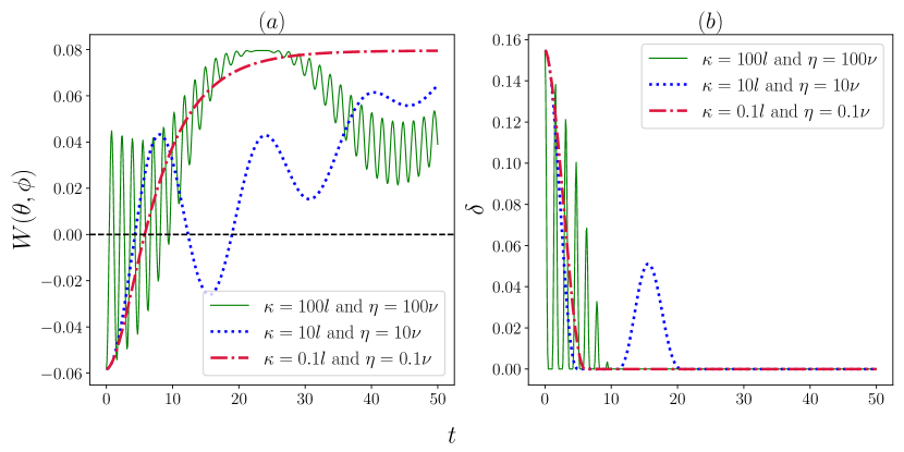
Figure 1: Variation of (a) Wigner function $W(\theta,\phi)$ and (b) nonclassical volume $\delta$ with time for the evolution of a single-qubit system via phase covariant channel. In (a), $\theta=\frac{\pi}{3}$ and $\phi=\pi$. The initial state is taken to be $\frac{1}{2}\ket{0}+\frac{\sqrt{3}}{2}\ket{1}$. The solid and dotted lines in both subplots have $l=g=0.01$, dot-dashed lines in both subplots have $l=g=1$.

To quantify the nonclassicality of the system, we use the nonclassical volume given by Eq. (6). Figure 1(b) illustrates the temporal evolution of the nonclassical volume $\delta$ for the intiale state $\frac{1}{2}\ket{0}+\frac{\sqrt{3}}{2}\ket{1}$ under the phase-covariant channel [Eq. (10)]. We observe that the nonclassical volume is non-zero during evolution but decreases over time. As shown in the figure, the nonclassical volume goes to zero. However, due to non-Markovian effects, it revives, indicating a temporary return of quantum coherence and interference effects. Here, we have taken a combination of NMAD and NMRTN channels. For the NMAD channel, the conditions for non-Markovian behavior is $l<2\kappa$, and for the NMRTN channel, the conditions for non-Markovian behavior is $\left(\frac{2\nu}{\eta}\right)^{2}>1$. The time evolution of the Wigner function, Fig. 1(a), clearly demonstrates that in the non-Markovian regime (as indicated by dotted blue and solid green lines), the Wigner function becomes negative multiple times. The frequency of oscillations is very high when $\kappa,\nu\gg l,\eta$. Additionally, the time evolution of nonclassical volume, Fig. 1(b), shows that the system’s memory effects can revive its nonclassicality. In the Markovian regime (dot-dashed red line), the nonclassical volume decays sharply.

Next, we study the speed of evolution of the single-qubit system evolving under the phase covariant channel. To this end, we use the QSL time $\tau^{W}_{QSL}$, henceforth denoted by $\tau_{QSL}$ for simplicity, defined using the Wasserstein-1-distance. The form of $\tau_{QSL}$ is given in Eq. (9). We take the initial state of the single qubit system to be $\frac{1}{\sqrt{2}}\left(\ket{0}+\ket{1}\right)$ and feed this and its time-evolved counterpart’s Wigner function into Eq. (II.3) to calculate the numerator in the expression of $\tau_{QSL}$. Further, we take the time average of the Wasserstein-1-norm of the time derivative of the Wigner function for the above state at any time $t$, using Eq. (13). This time average is the average velocity of the system’s evolution for the given driving time, and it constitutes the denominator of $\tau_{QSL}$.

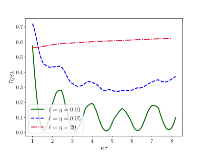
Figure 2: Variation of QSL time $\tau_{QSL}$ with qubit-environment coupling strength $\kappa$ for the system’s evolution under phase-covariant channel in the non-Markovian regime. Here, $\nu=\kappa$. The driving time $\tau$ is taken to be one. The initial state is taken to be $\frac{1}{\sqrt{2}}\left(\ket{0}+\ket{1}\right)$.

The variation of $\tau_{QSL}$ with qubit-environment coupling strength $\kappa$ for the evolution of the single-qubit system under phase covariant channel using Wasserstein-1-distance is plotted in Fig. 2. In the non-Markovian regime (depicted by solid green and dotted blue lines), when $2\kappa,2\nu\gg l,\eta$, the system’s speed of evolution is very fast and oscillatory in nature, as the $\tau_{QSL}$ oscillates near the lowest value. Upon increasing the value of $\eta$ and $l$, the speed of evolution slows down, which increases as we increase the $\kappa$. Further, in the Markovian regime (depicted by the dot-dashed red line), the system’s speed of evolution decreases monotonically. This brings out that non-Markovianity aids in speeding up the evolution.

III.2 QSL time for the evolution of the two-qubit dissipative model using Wigner function

Here, we analyze the Wigner function, non-classical volume, and the evolution of the QSL time for a two-qubit initial separable state evolving under a squeezed thermal bath, as discussed above. We take the squeezing angle to be $\phi=0$, and $k_{0}=1$, $\omega_{0}=1$, $\Gamma_{j}=0.05$ and $\mu.r_{ij}=0$.

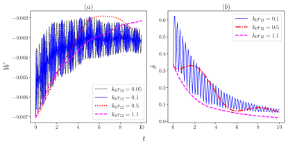
Figure 3: Variation of the (a) Wigner function $W(t)$ and (b) nonclassical volume $\delta$ with time $t$ for a two-qubit state ($\ket{01}$) under a squeezed thermal bath. Here, we have taken $\theta_{1}=\frac{\pi}{4}$, $\theta_{2}=\frac{\pi}{6}$, $\phi_{1}=\frac{\pi}{8}$, $\phi_{2}=\frac{\pi}{6}$ for (a). For both (a) and (b), temperature $T=1$, bath squeezing parameters $r=-0.2$ and $\phi=0$. Further, $\omega_{1}=\omega_{2}=1$ and $\Gamma_{1}=\Gamma_{2}=0.05$.

Figure 3(a) illustrates the time-dependent variation of the Wigner function for a two-qubit initial state $\ket{01}$ under the influence of a squeezed thermal bath at different inter-qubit distances. We observe that the Wigner function exhibits negative and oscillatory behavior at small inter-qubit distances (collective regime). However, as the inter-qubit distance increases, the Wigner function oscillations cease, though still remaining negative. Figure 3(b) depicts the variation of the nonclassical volume $\delta$ as a function of time for the evolution of a two-qubit initial separable state mentioned above. The plot reveals that the nonclassical volume oscillates and decreases over time. However, as the inter-qubit distance increases, these oscillations diminish. This behavior is similar to the behavior of the Wigner function under similar conditions. This shows that the behavior in the collective regime is non-Markovian in nature.

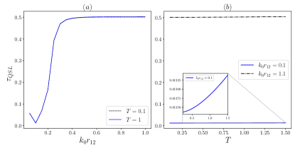
Figure 4: Variation of QSL time $\tau_{QSL}$ with (a) $k_{0}r_{12}$ at two different temperatures $T=0.1$ and $T=1$ and (b) $T$ for two inter-qubit distances $k_{0}r_{12}=0.1$ and $k_{0}r_{12}=1.1$. The initial two-qubit state ($\ket{01}$) is evolved under a squeezed thermal bath with bath squeezing parameters $r=-0.2$ and $\phi=0$. The actual driving time is $\tau=0.5$. The other parameters are taken to be $\omega_{1}=\omega_{2}=1$ and $\Gamma_{1}=\Gamma_{2}=0.05$.

In Fig. 4(a), we plot the variation of the QSL time as a function of the inter-qubit distance for an initial state $\ket{01}$ under a squeezed thermal bath at different temperatures. The QSL time shows a similar pattern of peaks and valleys for different temperatures. However, the values of QSL time are slightly higher for higher temperatures. The corresponding variation as a function of temperature for different inter-qubit distances is plotted in Fig. 4(b). As evident, the evolution is faster in the collective regime (bold curve) as compared to that in the independent regime (dot-dashed curve). It is known that entanglement is generated from the separable state in this model in the collective regime [59, 61]. The above plots benchmark the fact that due to the generation of the entanglement, the speed of the evolution is faster [30].

To study the impact of the evolution on the correlation between the two qubits, we study the quantum discord together with the QSL time. To this end, we take the Werner state as the system’s initial state. The two-qubit Werner state is given by [66]

$$\rho_{W_{AB}}=P|\psi\rangle\langle\psi|+\frac{1-P}{4}\mathbb{I},$$ (26)

where $|\psi\rangle=\sqrt{\frac{1}{2}}\left(|00\rangle+|11\rangle\right)$ and $P$ is the mixing probability such that $0\leq P\leq 1$. Furthermore, we study the quantum correlations using quantum discord [67], which is defined as

$$\mathit{D}\left(A:B\right)=S\left(B\right)-S\left(A,B\right)+S\left(A|B\right),$$ (27)

where $S(A)$ and $S(B)$ are the von Neumann entropies of the subsystem states $\rho_{A}$ and $\rho_{B}$, respectively. The terms $S(A,B)$ and $S(A|B)$ are the joint von Neumann entropy and the quantum conditional entropy of the system, respectively. The quantum conditional entropy $S(A|B)$ is given by

$$S\left(A|B\right)=\min_{\{\prod_{k}\}}\sum_{k=1}^{\mathit{H}_{B}}p_{k}S(\rho_{A|\prod_{k}}),$$ (28)

where $\mathit{H}_{B}$ is the Hilbert space dimension of subsystem $B$. $\rho_{A|\Pi_{k}}$ is the post-measurement state for the subsystem $A$ when a measurement is performed on the subsystem $B$ and $p_{k}=\text{Tr}({\Pi_{k}}^{\dagger}\Pi_{k}\rho_{AB})$ is the probability associated with the measurement operators $\Pi_{k}$. $\rho_{A|\Pi_{k}}$ can be explicitly written as

$$\rho_{A|\prod_{k}}=\frac{1}{p_{k}}\text{Tr}_{B}\left(\Pi_{k}\rho_{AB}\Pi_{k}\right).$$ (29)

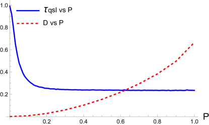
Figure 5: Variation of QSL time $\tau_{QSL}$ and quantum discord $D$ with mixing parameter $P$ for the Werner state under a squeezed thermal bath with bath squeezing parameters $r=0.5$ and $\phi=0$ for inter-atomic distances $k_{0}r_{ij}=0.05$, $T=1$ and $\tau=1$.

We calculate the quantum discord and QSL time as a function of the mixing probability $P$ and plot them in Fig. 5. An initial rapid decay in the QSL time is observed as we increase the value of the $P$. The QSL time saturates for values of $P$ greater than 0.2. It has the highest value when the state is a separable maximally mixed state and the lowest when it is maximally entangled ($P=1$). This reiterates that the speed of evolution is faster when quantum correlations increase, which is consistent with what was observed in [30]. Quantum discord shows a monotonically increasing behavior. At $P=1$, the Werner state becomes the Bell state, which should have the maximum value of discord, that is, one. However, due to the interaction of the thermal bath with the two-qubit system, the value of quantum discord is lower than one at $P=1$.

IV Conclusions

Here, we focused on the quantum speed limit using the Wigner function. This had the advantage of computational simplicity and provided a visualization of quantum to classical transition. The scenarios examined were a single-qubit system evolving under the phase covariant channel and a two-qubit system interacting with a squeezed thermal bath with position-dependent coupling. We investigated the Wigner function, non-classical volume, and speed limit for both models. The negative values of the Wigner function and non-zero nonclassical volume depicted the quantumness of the above systems. The non-Markovian region in the phase covariant model was found to favor the rebirth of nonclassicality in the system as well as the system’s speed of evolution. The oscillations of the Wigner function and the nonclassical volume observed in the collective regime of the two-qubit model point to the non-Markovian behavior there. The inter-qubit distance in the two-qubit dissipative model had an interesting role in the system’s evolution. It was observed for the two-qubit model that the collective regime was conducive to speeding up the evolution. This could be attributed to the generation of quantum correlations in this regime, such as entanglement and quantum discord. Further, with an increment in the temperature, the system slowed down.

References

- Banerjee [2018] S. Banerjee, Open Quantum Systems: Dynamics of Nonclassical Evolution, Texts and Readings in Physical Sciences (Springer Nature Singapore, 2018).
- Breuer and Petruccione [2002] H.-P. Breuer and F. Petruccione, The theory of open quantum systems (OUP Oxford, 2002).
- Breuer et al. [2016] H.-P. Breuer, E.-M. Laine, J. Piilo, and B. Vacchini, Reviews of Modern Physics 88, 021002 (2016).
- Zhang et al. [2012] W.-M. Zhang, P.-Y. Lo, H.-N. Xiong, M. W.-Y. Tu, and F. Nori, Physical review letters 109, 170402 (2012).
- Carmichael [2009] H. Carmichael, An open systems approach to quantum optics: lectures presented at the Université Libre de Bruxelles, October 28 to November 4, 1991, Vol. 18 (Springer Science & Business Media, 2009).
- Daley [2014] A. J. Daley, Advances in Physics 63, 77 (2014).
- Sieberer et al. [2016] L. M. Sieberer, M. Buchhold, and S. Diehl, Reports on Progress in Physics 79, 096001 (2016).
- Kosloff [2013] R. Kosloff, Entropy 15, 2100 (2013).
- de Vega and Alonso [2017] I. de Vega and D. Alonso, Rev. Mod. Phys. 89, 015001 (2017).
- Kumar et al. [2018] N. P. Kumar, S. Banerjee, R. Srikanth, V. Jagadish, and F. Petruccione, Open Systems & Information Dynamics 25, 1850014 (2018).
- Acín et al. [2018] A. Acín, I. Bloch, H. Buhrman, T. Calarco, C. Eichler, J. Eisert, D. Esteve, N. Gisin, S. J. Glaser, F. Jelezko, et al., New Journal of Physics 20, 080201 (2018).
- Kurizki et al. [2015] G. Kurizki, P. Bertet, Y. Kubo, K. Mølmer, D. Petrosyan, P. Rabl, and J. Schmiedmayer, Proceedings of the National Academy of Sciences 112, 3866 (2015).
- Koch [2016] C. P. Koch, Journal of Physics: Condensed Matter 28, 213001 (2016).
- Robertson [1929] H. P. Robertson, Physical Review 34, 163 (1929).
- Hegerfeldt [2013] G. C. Hegerfeldt, Physical review letters 111, 260501 (2013).
- Mandelstam [1945] L. Mandelstam, J. Phys.(USSR) 9, 249 (1945).
- Margolus and Levitin [1998] N. Margolus and L. B. Levitin, Physica D: Nonlinear Phenomena 120, 188 (1998).
- Sun et al. [2019] S. Sun, Y. Zheng, et al., Physical Review Letters 123, 180403 (2019).
- Ness et al. [2022] G. Ness, A. Alberti, and Y. Sagi, Physical Review Letters 129, 140403 (2022).
- Haseli and Salimi [2020] S. Haseli and S. Salimi, Laser Physics Letters 17, 105201 (2020).
- Anandan and Aharonov [1990] J. Anandan and Y. Aharonov, Phys. Rev. Lett. 65, 1697 (1990).
- Pati [1991] A. K. Pati, Physics Letters A 159, 105 (1991).
- Anandan and Pati [1997] J. S. Anandan and A. K. Pati, Physics Letters A 231, 29 (1997).
- Giovannetti et al. [2003] V. Giovannetti, S. Lloyd, and L. Maccone, Phys. Rev. A 67, 052109 (2003).
- Deffner and Campbell [2017] S. Deffner and S. Campbell, Journal of Physics A: Mathematical and Theoretical 50, 453001 (2017).
- del Campo et al. [2013] A. del Campo, I. L. Egusquiza, M. B. Plenio, and S. F. Huelga, Physical review letters 110, 050403 (2013).
- Deffner and Lutz [2013] S. Deffner and E. Lutz, Physical review letters 111, 010402 (2013).
- Aggarwal et al. [2022] S. Aggarwal, S. Banerjee, A. Ghosh, and B. Mukhopadhyay, New Journal of Physics 24, 085001 (2022).
- Baruah et al. [2023] R. Baruah, K. Paulson, and S. Banerjee, Annalen der Physik 535, 2200199 (2023).
- Tiwari et al. [2023] D. Tiwari, K. G. Paulson, and S. Banerjee, Annalen der Physik 535, 2200452 (2023), https://onlinelibrary.wiley.com/doi/pdf/10.1002/andp.202200452 .
- Campo et al. [2014] A. d. Campo, J. Goold, and M. Paternostro, Scientific Reports 4 (2014), 10.1038/srep06208.
- Julià-Farré et al. [2020] S. Julià-Farré, T. Salamon, A. Riera, M. N. Bera, and M. Lewenstein, Phys. Rev. Res. 2, 023113 (2020).
- Mohan and Pati [2021] B. Mohan and A. K. Pati, Phys. Rev. A 104, 042209 (2021).
- Tiwari and Banerjee [2023] D. Tiwari and S. Banerjee, Frontiers in Quantum Science and Technology 2 (2023), 10.3389/frqst.2023.1207552.
- Bouri et al. [2024] S. Bouri, A. K. Jha, and S. Banerjee, “Probing cp violation and mass hierarchy in neutrino oscillations in matter through quantum speed limits,” (2024), arXiv:2405.13114 [hep-ph] .
- Banerjee and Paulson [2023] S. Banerjee and K. G. Paulson, The European Physical Journal Plus 138 (2023), 10.1140/epjp/s13360-023-04228-2.
- Ashhab et al. [2012] S. Ashhab, P. C. de Groot, and F. Nori, Phys. Rev. A 85, 052327 (2012).
- Bekenstein [1981] J. D. Bekenstein, Phys. Rev. Lett. 46, 623 (1981).
- Paulson et al. [2022] K. G. Paulson, S. Banerjee, and R. Srikanth, Quantum Information Processing 21 (2022), 10.1007/s11128-022-03675-7.
- Lloyd [2000] S. Lloyd, Nature 406, 1047–1054 (2000).
- Zwierz et al. [2010] M. Zwierz, C. A. Pérez-Delgado, and P. Kok, Phys. Rev. Lett. 105, 180402 (2010).
- Giovannetti et al. [2011] V. Giovannetti, S. Lloyd, and L. Maccone, Nature Photonics 5, 222–229 (2011).
- Caneva et al. [2009] T. Caneva, M. Murphy, T. Calarco, R. Fazio, S. Montangero, V. Giovannetti, and G. E. Santoro, Phys. Rev. Lett. 103, 240501 (2009).
- Liegener and Łukasz Rudnicki [2022] K. Liegener and Łukasz Rudnicki, Classical and Quantum Gravity 39, 12LT01 (2022).
- Wei et al. [2023] Z.-D. Wei, W. Han, Y.-J. Zhang, S.-J. Du, Y.-J. Xia, and H. Fan, Phys. Rev. D 108, 126011 (2023).
- Stratonovich [1956] R. L. Stratonovich, Soviet Physics JETP 31, 1012 (1956).
- Agarwal [2012] G. S. Agarwal, Quantum Optics (Cambridge University Press, 2012).
- Thapliyal et al. [2015] K. Thapliyal, S. Banerjee, A. Pathak, S. Omkar, and V. Ravishankar, Annals of Physics 362, 261 (2015).
- Thapliyal et al. [2016] K. Thapliyal, S. Banerjee, and A. Pathak, Annals of Physics 366, 148 (2016).
- Hillery et al. [1984] M. Hillery, R. O’Connell, M. Scully, and E. Wigner, Physics Reports 106, 121 (1984).
- Wigner [1932a] E. Wigner, Physical Review 40, 749 – 759 (1932a), cited by: 7763.
- Arkhipov et al. [2018] I. I. Arkhipov, A. Barasiński, and J. Svozilík, Scientific reports 8, 16955 (2018).
- Semenov et al. [2006] A. Semenov, D. Y. Vasylyev, and B. Lev, Journal of Physics B: Atomic, Molecular and Optical Physics 39, 905 (2006).
- Genoni et al. [2013] M. G. Genoni, M. L. Palma, T. Tufarelli, S. Olivares, M. Kim, and M. G. Paris, Physical Review A 87, 062104 (2013).
- Deffner [2017] S. Deffner, New Journal of Physics 19, 103018 (2017).
- Smirne et al. [2016] A. Smirne, J. Kołodyński, S. F. Huelga, and R. Demkowicz-Dobrzański, Phys. Rev. Lett. 116, 120801 (2016).
- Teittinen et al. [2018] J. Teittinen, H. Lyyra, B. Sokolov, and S. Maniscalco, New Journal of Physics 20, 073012 (2018).
- Filippov et al. [2020] S. N. Filippov, A. N. Glinov, and L. Leppäjärvi, Lobachevskii Journal of Mathematics 41, 617–630 (2020).
- Banerjee et al. [2010] S. Banerjee, V. Ravishankar, and R. Srikanth, Annals of Physics 325, 816 (2010).
- Ficek and Tanaś [2002] Z. Ficek and R. Tanaś, Physics Reports 372, 369 (2002).
- Banerjee et al. [2009] S. Banerjee, V. Ravishankar, and R. Srikanth, The European Physical Journal D 56, 277–290 (2009).
- Wigner [1932b] E. Wigner, Phys. Rev. 40, 749 (1932b).
- Varshalovich et al. [1988] D. A. Varshalovich, A. N. Moskalev, and V. K. Khersonskii, Quantum theory of angular momentum (World Scientific, 1988).
- Kenfack and Życzkowski [2004] A. Kenfack and K. Życzkowski, Journal of Optics B: Quantum and Semiclassical Optics 6, 396 (2004).
- Wasserstein [1969] L. N. Wasserstein, Problems Inf. Transm. 5, 47 (1969).
- Werner [1989] R. F. Werner, Phys. Rev. A 40, 4277 (1989).
- Ollivier and Zurek [2001] H. Ollivier and W. H. Zurek, Phys. Rev. Lett. 88, 017901 (2001).