Repeating Partial Tidal Encounters of Sun-like Stars Leading to their Complete Disruption

Abstract

Stars grazing supermassive black holes (SMBHs) on bound orbits may produce periodic flares over many passages, known as repeating partial tidal disruption events (TDEs). Here we present 3D hydrodynamic simulations of sun-like stars over multiple tidal encounters. The star is significantly restructured and becomes less concentrated as a result of mass loss and tidal heating. The vulnerability to mass loss depends sensitively on the stellar density structure, and the strong correlation between the fractional mass loss $\Delta M/M_{*}$ and the ratio of the central and average density $\rho_{\mathrm{c}}/\bar{\rho}$, which was initially derived in disruption simulations of main-sequence stars, also applies for stars strongly reshaped by tides. Over multiple orbits, the star loses progressively more mass in each encounter and is doomed to a complete disruption. Throughout its lifetime, the star may produce numerous weak flares (depending on the initial impact parameter), followed by a couple of luminous flares whose brightness increases exponentially. Flux-limited surveys are heavily biased towards the brightest flares, which may appear similar to the flare produced by the same star undergoing a full disruption on its first tidal encounter. This places new challenges on constraining the intrinsic TDE rates, which needs to take repeating TDEs into account. Other types of stars with different initial density structure (e.g., evolved stars with massive cores) follow distinct evolution tracks, which might explain the diversity of the long-term luminosity evolution seen in recently uncovered repeaters.

1 Introduction

The principal way in which supermassive black holes (SMBHs) have been studied observationally is via the emission of gas that slowly inspirals onto the SMBH. These steady-state active galactic nuclei (AGN) are typically fed by gas that originates far from the SMBH itself, resulting in a feeding rate that varies little over decades (e.g., Auchettl et al., 2017, 2018; Frederick et al., 2019; Dodd et al., 2021; Gezari, 2021). While they are magnificent laboratories to study the behavior of matter in extreme environments, as the environmental conditions (e.g., accretion rates) of each system are fixed in time, we typically require demographic study on an ensemble of AGNs (e.g., Merloni et al., 2003; Falcke et al., 2004; Wang et al., 2006). It can also be challenging to disentangle variations due to external quantities from variations due to SMBH properties. Furthermore, for the nearest SMBHs, including the one at the center of our own galaxy (e.g., Narayan et al., 1998), the paucity of gas in the local universe results in a tepid release of energy, hindering study on these dormant SMBHs.

This behavior is in stark contrast to the frantic evolution experienced by an SMBH that has recently disrupted a star through tides (Hills, 1975; Rees, 1988; Guillochon & Ramirez-Ruiz, 2013). When a star comes within a critical distance to a BH, immense tidal forces can remove a significant fraction, if not all, of the star’s mass, resulting in a stream of debris that falls back onto the BH and powers a luminous flare lasting for months. The disruption of stars by SMBHs has been linked to more than a dozen optical/X-ray transients (tidal disruption events; TDEs) in the cores of galaxies out to $z\approx 1$ (Gezari, 2021; van Velzen et al., 2021; Andreoni et al., 2022; Yao et al., 2023). The relatively short evolution timescale enables the study of the same SMBH subjected to different external conditions, which may transition between different modes of accretion (Abramowicz & Fragile, 2013; Wevers et al., 2021).

In the standard picture, the star is disrupted on a relatively weakly bound (nearly parabolic) orbit. Approximately half of the material removed from the star becomes bound to the SMBH (Rees, 1988), which is distributed into many different orbits, and falls back to the SMBH over a range of times (Evans & Kochanek, 1989; Phinney, 1989; De Colle et al., 2012; Guillochon & Ramirez-Ruiz, 2013). The rate that the material returns to the SMBH is characterized by three phases: a rapid rise to peak over a period of days, followed by relatively constant feeding over a period of weeks, and finally a power-law decay that can persist for decades – these timescales mainly depend on the mass of the SMBH (Mockler et al., 2019).

This picture can be dramatically altered if disrupted stars are placed on highly bound orbits (Hayasaki et al., 2018; Kıroğlu et al., 2023; Liu et al., 2023a), especially if they are not completely destroyed in the first pericenter passage. Such periodic encounters can give rise to repeating flares, which have been recently uncovered in synoptic surveys, such as ASASSN-14ko (Payne et al., 2021, 2022); eRASSt J045650.3–203750 (Liu et al., 2023b); AT 2018fyk (Wevers et al., 2019, 2023); RX J133157.6–324319.7 (Hampel et al., 2022; Malyali et al., 2023); AT 2020vdq (Somalwar et al., 2023); Swift J023017.0+283603 (Evans et al., 2023; Guolo et al., 2024), and AT 2022dbl (Lin et al., 2024). All these candidates repeat/rebrighten at a timescale from months to years, and our ability to detect longer-period repeaters is strongly limited by the span of surveys.

While most numerical work has focused on a single tidal encounter, the multiple-passage simulation space remains largely uncharacterized. Previous attempts to model a star surviving multiple tidal encounters rely on analytical recipes (MacLeod et al., 2013, 2014; Liu et al., 2023a) or fitting formula from hydrodynamic stellar libraries of single encounters (Broggi et al., 2024) for the star’s response to tidal interaction. These approaches cannot characterize the star’s tidal deformation and the mass loss coherently over time. In this Letter, we present 3D hydrodynamic simulations of multi-orbit encounters between a sun-like star and an SMBH, in which we track the structural evolution of the star and the long-term trend of mass loss over multiple encounters.

The Letter is organized as follows. In Section 2 we elaborate the necessity of hydrodynamic simulations and our model setups. In Section 3 we present the evolution of the star’s density structure over time, and the amount of mass removed in each tidal encounter. This is followed by our implications on the long-term trend of luminosity in these repeaters in Section 4. Finally in Section 5 we discuss how the initial structure of the star affects the behavior of the observed repeater, and address the challenges of inferring the TDE rates both theoretically and observationally, with the existence of an underlying population of repeating partial TDEs. We draw our conclusions in Section 6.

2 Simulating Multiple Tidal Encounters

2.1 Hydrodynamic Simulations

In both full and partial TDEs, the mass fallback rate $\dot{M}$ onto the SMBH depends on the distribution of the orbital energy, $\mathrm{d}M/\mathrm{d}E$, within the debris tail bound to the SMBH (Rees, 1988; Evans & Kochanek, 1989; Phinney, 1989; Guillochon & Ramirez-Ruiz, 2013),

$$\dot{M}=\frac{2}{3}\frac{\mathrm{d}M}{\mathrm{d}E}\left(\frac{\pi^{2}G^{2}M_{\mathrm{BH}}^{2}}{2}\right)^{1/3}t^{-5/3}.$$ (1)

The energy distribution in the debris, and thus $\dot{M}$, depend sensitively on the mass and age of the star as well on its pre-disruption orbital properties (e.g, Law-Smith et al., 2019, 2020). Hydrodynamic simulations are required to handle both the fluid dynamics within the debris tail and the gravitational interaction with the surviving core (Rosswog et al., 2008, 2009; Ramirez-Ruiz & Rosswog, 2009; Lodato et al., 2009; Coughlin & Nixon, 2019; Miles et al., 2020). The structure of the surviving star is also strongly deformed, which governs its behavior in subsequent encounters. Hydrodynamic simulations have to be employed to model the star’s response to mass loss (MacLeod et al., 2013; Ryu et al., 2020a), tidal excitation which deposits energy to the stellar interior (Li & Loeb, 2013; Manukian et al., 2013), and the re-accretion of marginally bound material as the star recedes from the pericenter to a region with a weaker tidal field (Faber et al., 2005; Guillochon et al., 2011; Antonini et al., 2011). In this work, our simulations focus on the evolution of the star’s structure following a series of tidal encounters.

We follow the approach of Liu et al. (2023a) and Law-Smith et al. (2019, 2020) to simulate a sun-like star over multiple orbits. The initial density profiles of a sun-like star are modeled with the Modules for Experiments in Stellar Astrophysics (MESA; Paxton et al., 2011), using the same setup presented in Law-Smith et al. (2019). As an outcome the stellar radius $R$ is 1.03 $\mathrm{R_{\odot}}$ at an age of 44.5 Gyr. The profile is then mapped to a 3D adaptive-mesh refinement (AMR) hydrodynamics code FLASH (Fryxell et al., 2000). The adiabatic index of the gas is $\Gamma=5/3$. We adopt a $10^{6}\,\mathrm{M_{\odot}}$ SMBH, but the results are scalable to other $M_{\mathrm{BH}}$. The major difference in the setups from Liu et al. (2023a) and Law-Smith et al. (2019, 2020) is the much smaller domain size adopted (100 $\mathrm{R_{\odot}}$ v.s. 1000 $\mathrm{R_{\odot}}$). Our zoom-in simulations prioritize the resolution within the star at the expense of not modeling the extended tidal tails.

We study orbits with three initial impact parameters, $\beta_{\mathrm{init}}=0.5$, 0.6, and 1.0, where $\beta$, the ratio of the tidal radius $r_{\mathrm{T}}\equiv R_{*}(M_{\mathrm{BH}}/M_{*})^{1/3}$ and the pericenter distance $r_{\mathrm{p}}$, characterizes how deep the star penetrates the tidal radius. These values are well below the critical $\beta_{\mathrm{crit}}$ for a full disruption (Mainetti et al., 2017a; Law-Smith et al., 2020; Ryu et al., 2020b), so the star can survive at least a couple of orbits. We also ensure that all the encounters are non-relativistic ($r_{\mathrm{p}}\gtrsim 50\,r_{\mathrm{g}}$, whereas we expect non-negligible relativistic effects when $r_{\mathrm{p}}\lesssim 10\,r_{\mathrm{g}}$; e.g., Laguna et al., 1993; Cheng & Bogdanović, 2014; Servin & Kesden, 2017; Tejeda et al., 2017; Gafton & Rosswog, 2019; Stone et al., 2019; Ryu et al., 2020c). We begin the simulation by relaxing the star onto the grid for 5 dynamical timescales ($t_{\mathrm{dyn}}=1664$ s), $10\,r_{\mathrm{T}}$ away from the SMBH before starting the eccentric orbital evolution. For the $\beta_{\mathrm{init}}=0.6$ and $1.0$ models the eccentricity $e$ is set to be 0.9, so the orbital periods $P_{\mathrm{orb}}$ are $\approx$400 $t_{\mathrm{dyn}}$ and $\approx$200 $t_{\mathrm{dyn}}$ each, corresponding to a couple of days. For the $\beta=0.5$ model we adopt a smaller $e=0.8$ for efficiency, and the period is same as that of the $\beta=1.0$ model. Liu et al. (2023a) have shown that $\mathrm{d}M/\mathrm{d}E$ is not significantly different for disruption on highly eccentric ($e\gtrsim 0.9$) or parabolic orbits ($e=1$). In reality $P_{\mathrm{orb}}$ is usually much longer ($e$ closer to unity), which brings the caveat that the star in the $\beta_{\mathrm{init}}=0.5$ model would suffer stronger tidal effects than the same star on an orbit with the same $\beta_{\mathrm{init}}$ but a longer $P_{\mathrm{orb}}$.

We stop the simulations when (i) $\Delta M/M_{*}>50\%$, when we usually expect the orbit of the remnant to be strongly altered (Gafton et al., 2015); or (ii) the star survives 10 orbits around the SMBH. We calculate the specific self binding energy $E_{*}$ in an iterative approach following Equations (2) and (3) in Guillochon & Ramirez-Ruiz (2013). The remaining stellar mass $M_{*}$ is the sum of mass in cells with $E_{*}<0$. The mass loss $\Delta M$ in each passage is defined as the decrease in $M_{*}$ in one orbit (as the star returns to $r=10\,r_{\mathrm{T}}$), unless $M_{*}\to 0$ beforehand. In practice we find $\Delta M$ stabilizes within $\approx$100 $t_{\mathrm{dyn}}$ after the previous encounter, and the variation in $\Delta M$ afterwards is $\lesssim$$10^{-6}\,\mathrm{M_{\odot}}$ per $t_{\mathrm{dyn}}$ before the next encounter.

At the end of our simulations, we find that the $\beta_{\mathrm{init}}=0.5$ model still retains $\approx$0.9 $\mathrm{M_{\odot}}$ of bound mass, while the $\beta_{\mathrm{init}}=0.6$ and 1.0 models are fully disrupted after 6 and 3 passages. The stellar parameters at each passage are listed in Table 1. In Figure 1 we show snapshots of the star in the $\beta_{\mathrm{init}}=0.6$ model, when the orbital separation is $10\,r_{\mathrm{T}}$ before each of its 6 pericenter passages. The central density $\rho_{\mathrm{c}}$ of the star decreases over time as a result of tidal energy injection, and the star expands. A diffuse envelope of marginally bound material is developed after the first encounter, which also keeps heating the stellar surface via re-accretion (Guillochon et al., 2011; MacLeod et al., 2013). But as the mass of this marginally bound envelope is tiny ($\lesssim$$10^{-3}\,\mathrm{M_{\odot}}$), it cannot influence the regeneration of the star.

Table 1: Stellar parameters in each encounter and the corresponding mass loss.

$\beta_{\mathrm{init}}$	$N_{\mathrm{passage}}$	$R_{*}$	$\rho_{\mathrm{c}}$	$\rho_{\mathrm{c}}/\bar{\rho}$	$\exp[(\beta/\beta_{\mathrm{crit}})^{\alpha}-1]$	$\Delta M$
		$(\mathrm{R_{\odot}})$	($\mathrm{g\,cm^{-3}}$)			$(10^{-2}\,\mathrm{M_{\odot}})$
0.5	1†	$1.03\pm 0.01$	143.7	$109\pm 3$	$0.758\pm 0.001$	$0.001\pm 0.015$
	2†	$1.21\pm 0.01$	56.9	$71\pm 2$	$0.774\pm 0.001$	$0.14\pm 0.05$
	3†	$1.33\pm 0.03$	42.7	$70\pm 4$	$0.787\pm 0.003$	$0.37\pm 0.09$
	4	$1.40\pm 0.05$	35.8	$70\pm 8$	$0.795\pm 0.006$	$0.57\pm 0.13$
	5	$1.43\pm 0.05$	31.2	$65\pm 6$	$0.798\pm 0.005$	$0.77\pm 0.17$
	6	$1.45\pm 0.05$	27.8	$61\pm 6$	$0.801\pm 0.006$	$0.99\pm 0.20$
	7	$1.47\pm 0.05$	25.0	$57\pm 6$	$0.804\pm 0.005$	$1.31\pm 0.23$
	8	$1.50\pm 0.06$	22.6	$56\pm 6$	$0.808\pm 0.006$	$1.66\pm 0.26$
	9	$1.53\pm 0.07$	20.6	$55\pm 8$	$0.812\pm 0.007$	$2.09\pm 0.29$
	10	$1.55\pm 0.07$	18.7	$53\pm 8$	$0.817\pm 0.007$	$2.71\pm 0.29$
0.6	1†	$1.03\pm 0.01$	143.7	$109\pm 3$	$0.779\pm 0.001$	$0.19\pm 0.07$
	2	$1.34\pm 0.02$	41.9	$71\pm 4$	$0.815\pm 0.002$	$1.32\pm 0.35$
	3	$1.51\pm 0.06$	29.9	$74\pm 9$	$0.836\pm 0.005$	$3.05\pm 0.62$
	4	$1.59\pm 0.09$	23.1	$69\pm 11$	$0.849\pm 0.007$	$5.41\pm 0.64$
	5	$1.90\pm 0.05$	9.5	$51\pm 4$	$0.895\pm 0.003$	$25.36\pm 0.81$
	6∗	$2.59\pm 0.15$	2.1	$39\pm 7$	$1.022\pm 0.001$	$65.97\pm 0.72$
1.0	1	$1.03\pm 0.01$	143.7	$109\pm 3$	$0.846\pm 0.001$	$8.10\pm 0.08$
	2	$1.72\pm 0.13$	50.4	$199\pm 44$	$0.920\pm 0.005$	$21.55\pm 0.19$
	3∗	$1.97\pm 0.15$	19.9	$153\pm 35$	$0.965\pm 0.003$	$56.74\pm 0.30$

Note. — Passages where there is unresolved numerical tidal dissipation are labeled by $\dagger$. Full disruptions are indicated by $*$.

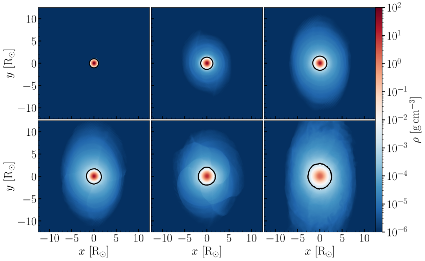
Figure 1: Density maps of the star on the $\beta_{\mathrm{init}}=0.6$ orbit before each of its 6 pericenter passages ($10\,r_{\mathrm{T}}$ from the SMBH). The black contour denotes the density threshold $\rho=10^{-3}$ g cm^-3, which we define as the stellar surface. The star expands over time and $\rho_{\mathrm{c}}$ drops. The stellar surface is continuously heated by the re-accretion of the marginally bound materials, which has a much greater $r_{\mathrm{T}}$ and will be easily removed in the subsequent encounter.

2.2 Adiabatic Mass Loss Approximation

Characterizing a star’s response to mass loss is critical in understanding the stability of mass transfer in binary systems. When the mass loss occurs at a timescale much shorter than the thermal timescale at the stellar surface, a common assumption is that the the star would react adiabatically within $t_{\mathrm{dyn}}$ (e.g., Hjellming & Webbink, 1987; Soberman et al., 1997). As a generalized interacting binary system, the long-term evolution of a star undergoing repeating partial TDEs has also been explored assuming adiabatic mass loss (MacLeod et al., 2013, 2014; Liu et al., 2023a). In this work, we also set up an adiabatic mass loss model in comparison with the fully hydrodynamic treatment, in order to quantify the importance of tides.

We start with the same MESA sun-like star model and remove a total mass of $0.1\,\mathrm{M_{\odot}}$ from its envelope via stellar wind at a constant rate of $10^{-6}\,\mathrm{M_{\odot}}\,\mathrm{yr^{-1}}$. The corresponding mass loss timescale is $10^{5}\,$yr, significantly lower than the thermal (Kelvin-Helmholtz) timescale ($\approx$$10^{7}$ yr) but much longer than the dynamical timescale ($\approx$hr). Throughout the evolution, the entropy profile remains nearly unchanged, except for that in the super-adiabatic stellar surface (see also Woods & Ivanova, 2011). While the mass loss rate seems to be specified here, the result is not sensitive to it – bumping up the mass loss rate ($10^{-5}\,\mathrm{M_{\odot}}\,\mathrm{yr^{-1}}$) has a minimal impact on the stellar structure when the same amount of total mass is removed.

2.3 Tidal Dissipation

Tidal forces alter the structure of the star by converting orbital energy into mechanical energy stored in oscillations. The energy deposited into these oscillations is roughly proportional to the square of their amplitude (Guillochon et al., 2011), $|{\delta E_{*}}/{E_{*}}|\approx(\delta R/R)^{2}$, where $|E_{*}|\simeq GM^{2}/R$ is the magnitude of the gravitational binding energy of the star. For weak tidal encounters in which $\delta R$ is below the resolution of the simulations, tides will be dissipated numerically, puffing up the star in an artificial way. In our simulations the typical cell size within the star is $\Delta L=0.025\,\mathrm{R_{\odot}}$. The energy deposition during a single passage is (Press & Teukolsky, 1977)

$$\delta E_{*}=\left(\frac{GM^{2}}{R}\right)\beta^{6}T(\beta),$$ (2)

where $T(\beta)$ also depends on the stellar structure. For a $\gamma=4/3$ polytrope, a good approximation of sun-like stars, $T(\beta)\approx 10^{-2}$–$10^{-1}$ for $\beta\approx 0.5$–1.0 (Ivanov & Novikov, 2001). For $\beta_{\mathrm{init}}=0.5$, in the first passage we have $|\delta E_{*}/E_{*}|\approx 10^{-4}$, requiring a cell size finer than $\approx$$0.01\,\mathrm{R_{\odot}}$, beyond our computational ability in multi-orbit simulations. This means we inevitably overestimate the energy deposition at the beginning of the simulation.

As star expands during subsequent passages, both $R_{*}$ and $\beta$ increase, easing the resolution requirement to resolve the tides. When a sun-like star has expanded to $R_{*}$ over multiple passages, our cell size $\Delta L$ must satisfy

$$\frac{\Delta L}{\mathrm{R_{\odot}}} \lesssim\beta^{3}\left(\frac{R_{*}}{\mathrm{R_{\odot}}}\right)T^{1/2}(\beta)$$

$$\simeq\beta_{\mathrm{init}}^{3}\left(\frac{R_{*}}{\mathrm{R_{\odot}}}\right)^{4}T\left[\beta_{\mathrm{init}}\left(\frac{R_{*}}{\mathrm{R_{\odot}}}\right)\right].$$

By adopting the analytical fit to $T(\beta)$ in Generozov et al. (2018), we solve $R_{\Delta L}$, the minimum $R_{*}$ to which the star must expand such that $\Delta L\simeq\delta R$, to be $\approx$1.4 $\mathrm{R_{\odot}}$, 1.2 $\mathrm{R_{\odot}}$, and 0.75 $\mathrm{R_{\odot}}$ for $\beta_{\mathrm{init}}=0.5$, 0.6, and 1.0. In Table 1 we mark the corresponding orbits with insufficient resolution. We will discuss this further in Section 3.

We note that numerical dissipation of the hydrodynamic scheme is the only dissipation mechanism in our simulations. Once $R_{*}$ exceeds $R_{\Delta L}$, we do not observe significant decay of the $l=2$ modes between pericenter passages. Consequently, the tidal modes remain excited and interfere with newly excited modes in the subsequent encounter (Mardling, 1995a, b). The response of the star during the following passage depends on the phase of the oscillations at pericenter, leading to a chaotic behavior. Therefore it is impossible to predict the exact number of orbits a star could survive before the complete disruption, which can be sensitive to small perturbations of orbital parameters (e.g., $\beta_{\mathrm{init}}$ and eccentricity; Guillochon et al., 2011). In realistic stars, the oscillation energy can be transferred from the primary $l=2$ mode to higher-order daughter modes via non-linear coupling (Kumar & Goodman, 1996; Weinberg et al., 2012), which can then be efficiently damped (e.g., via microscopic viscosity or turbulence) within the realistic orbital timescale ($\gtrsim$yr) of repeating TDEs, reducing the degree of chaos. Nevertheless, tidal dissipation remains an open problem, and is a source of uncertainty in our calculations.

3 The Star’s Response to Repeating Partial Disruptions

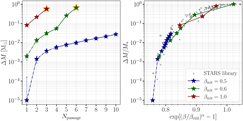
Figure 2: The mass $\Delta M$ unbound by the SMBH for 3 different $\beta_{\mathrm{init}}$. Left: $\Delta M$ at each passage. The uncertainty is given by the mass that is marginally bound to the star ($E_{*}<0$, $\rho<10^{-3}\mathrm{g\,cm^{-3}}$). Orange markers indicate full disruptions. Dash-dotted lines indicate that numerical tidal dissipation dominates the stellar evolution in the corresponding orbits. Right: fractional mass loss $\Delta M/M_{*}$ as a function of $\exp[(\beta/\beta_{\mathrm{crit}})^{\alpha}-1]$ (see text for the definition). Over-plotted are the results from the STARS library in Law-Smith et al. (2020), suggesting $\exp[(\beta/\beta_{\mathrm{crit}})^{\alpha}-1]$ well quantifies the vulnerability of the star to mass loss.

In partial TDEs, the fractional mass loss $\Delta M/M_{*}$ depends on the stellar structure. Ryu et al. (2020a) showed that $\Delta M/M_{*}$ can be quantified with $\beta$ and a physical tidal radius, $\mathcal{R}_{\mathrm{t}}$. Unlike $r_{\mathrm{T}}$ that depends on the average density of the star $\bar{\rho}$, $\mathcal{R}_{\mathrm{t}}$ depends on the ratio of the central density and the average, $\rho_{\mathrm{c}}/\bar{\rho}$ (Ryu et al., 2020d, b). Similarly, Law-Smith et al. (2020) defined

$$x\equiv\exp[(\beta/\beta_{\mathrm{crit}})^{\alpha}-1],$$ (3)

which also strongly correlates with $\Delta M/M_{*}$. Here $\alpha\equiv\left(\rho_{\mathrm{c}}/\bar{\rho}\right)^{-1/3}$, and $\beta_{\mathrm{crit}}$ is the critical impact parameter for full disruption, again depending on $\rho_{\mathrm{c}}/\bar{\rho}$,

$$\beta_{\mathrm{crit}}\simeq\left\{\begin{array}[]{cc}0.5(\rho_{\mathrm{c}}/\bar{\rho})^{1/3},&\rho_{\mathrm{c}}/\bar{\rho}\lesssim 500,\\ 0.39(\rho_{\mathrm{c}}/\bar{\rho})^{1/2.3},&\rho_{\mathrm{c}}/\bar{\rho}\gtrsim 500.\end{array}\right.$$ (4)

Here we show the relation between $\exp[(\beta/\beta_{\mathrm{crit}})^{\alpha}-1]$ and $\Delta M/M_{*}$ still holds even if the star has a profound tidal interaction history with its density structure being substantially perturbed.

Definitions of $R_{*}$ and $\bar{\rho}$ become tricky with the existence of the extended, thin envelope bound to the star. We find that at the end of relaxation phase, the density at the original surface $R=1.03\,\mathrm{R_{\odot}}$ is $\approx$$10^{-3}$ g cm^-3. We therefore define $R_{*}$ as the radius at which the average density is $10^{-3}$ g cm^-3 and evaluate $\bar{\rho}$ correspondingly. Additionally, tidal oscillations break the spherical symmetry of the star, and Ryu et al. (2020a) found that the surviving star can be substantially oblate. To account for the fluctuation at the surface, we evaluate both the mean and standard deviation of $\rho$ at a sequence of distances from the center, so we can define a confident interval of $R_{*}$ within which the density profile is in 1-$\sigma$ consistence with $10^{-3}$ g cm^-3.

In Figure 2 we show the mass loss $\Delta M$ during each passage for all three models. The uncertainty of $\Delta M$ is given by the marginally bound mass (typically $\approx$$10^{-4}$–$10^{-3}$ $\mathrm{M_{\odot}}$), which we define as bound material ($E_{*}<0$) outside $R_{*}$ ($\rho<10^{-3}\,\mathrm{g\,cm^{-3}}$). In all three models, as the star is continuously tidally heated, $\exp[(\beta/\beta_{\mathrm{crit}})^{\alpha}-1]$ increases over time, and the star gets progressively more vulnerable to disruption with $\Delta M$ going up roughly exponentially. On the right panel of Figure 2 we over-plot targets in the Stellar Tidal Disruption Events with Abundances and Realistic Structures (STARS) library from MESA main-sequence models of a wide range of stellar masses, ages, and orbital parameters (Law-Smith et al., 2020). Despite some chaos due to tidal modes excited in previous passages that have not been fully damped, our results still agree well with the trace of the STARS main-sequence stars. This confirms that $\rho_{\mathrm{c}}/\bar{\rho}$ is an ideal summary quantity in evaluating the $\Delta M/M_{*}$, regardless of the star’s mass loss and/or tidal interaction history.

In Figure 3 we show the evolution of $\exp[(\beta/\beta_{\mathrm{crit}})^{\alpha}-1]$ as the star loses mass in our hydrodynamic simulations and in the MESA model which only takes into account adiabatic mass loss. On the left panels we show the adiabatic evolution of $R_{*}$, $\rho_{\mathrm{c}}$, and $\bar{\rho}$ of the sun-like star. $R_{*}$ shrinks as the star is adiabatically stripped and $\rho_{\mathrm{c}}/\bar{\rho}$ drops over time, consistent with analytical results (e.g., Hjellming & Webbink, 1987; Dai et al., 2013). The net effect is a decreasing $\exp[(\beta/\beta_{\mathrm{crit}})^{\alpha}-1]$, meaning that while the star is getting less concentrated, its tidal radius shrinks even more rapidly. When $\exp[(\beta/\beta_{\mathrm{crit}})^{\alpha}-1]$ drops below $\approx$0.75, the star is effectively detached from the SMBH and the mass loss is ceased. This trend is opposite to what we find in hydrodynamic simulations, suggesting that tides play an critical role in injecting energy and reshaping the density structure of the star.

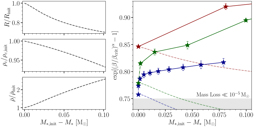
Figure 3: Models assuming adiabatic mass loss dramatically underestimate the vulnerability of the star to upcoming tidal disruptions. Left: the evolution of the stellar radius $R_{*}$, central density $\rho_{c}$, and average density $\bar{\rho}$ in a MESA model, when we adiabatically remove 0.1 $M_{\odot}$ from a sun-like star via a constant stellar wind. Right: $\exp[(\beta/\beta_{\mathrm{crit}})^{\alpha}-1]$ as a function of the total mass loss. Results from our hydrodynamic simulations are plotted again as pentagrams, while the dashed lines are how we expect the star to evolve on orbits of corresponding $\beta_{\mathrm{init}}$ using results from the adiabatic model. Dash-dotted lines again indicate overestimated tidal energy injection due to numerical dissipation in our simulations. These adiabatic tracks should not go below $\exp[(\beta/\beta_{\mathrm{crit}})^{\alpha}-1]\simeq 0.75$, when significant mass loss will not happen (see Figure 2).

In Section 2.3 we suggest that the number of orbits before a star reaches $R_{\Delta L}$ is chaotic, and dramatically underestimated in our simulations (indicated as dashed lines in Figure 2). For our $\beta_{\mathrm{init}}=0.5$ and 0.6 models, $R_{*}$ exceeds $R_{\Delta L}$ in 3 and 1 orbit(s). The number of actual orbits can be roughly estimated under an energy consideration. The mass loss when the star reaches $R_{\Delta L}$ is still minimal ($\lesssim$1%). Neglecting order unity coefficients, the increase in the total energy is

$$\Delta E_{*}\simeq\frac{G\mathrm{M^{2}_{\odot}}}{\mathrm{R_{\odot}}}\left(1-\frac{\mathrm{R_{\odot}}}{R_{\Delta L}}\right).$$ (5)

Assuming the tidal oscillations are damped efficiently, the number of orbits it requires to inject this amount of tidal energy is

$$N_{\mathrm{orb}}(R_{\Delta L})\simeq\frac{\Delta E_{*}}{\delta E_{*}}\approx\beta^{-6}T^{-1}(\beta)\left(1-\frac{\mathrm{R_{\odot}}}{R_{\Delta L}}\right).$$ (6)

This corresponds to $\approx$$10^{3}$ and $\approx$$10^{2}$ orbits for $\beta_{\mathrm{init}}=0.5$ and 0.6, respectively. As the star expands beyond $R_{\mathrm{\Delta L}}$, we are able to model the last few orbits when we expect most of the mass loss and the strongest flares. In Section 4 we will draw a sketch of the repeating flares as the stars step to the end of their lives.

4 Implications on Flare Evolution

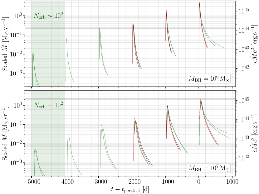
Figure 4: An illustration of mass fallback rates $\dot{M}(t)$ over flares for the $\beta_{\mathrm{init}}=0.6$ and 1.0 models, assuming two different $M_{\mathrm{BH}}$. The time is measured with respect to the last pericenter passage, which fully disrupts the star and produces the strongest flare. For each passage, we adopt fallback curves from their $\leq$3 nearest neighbors in the $\log(\Delta M/M)$ - $\exp[(\beta/\beta_{\mathrm{crit}})^{\alpha}-1]$ space from the STARS library (grey circles in Figure 2). When adopting those mass fallback curves, we assume neighbors would show similar $\dot{M}/M_{*}$, then scale $\dot{M}$ using the mass of the star before each passage in the hydrodynamic simulations. We overlay the mock luminosity assuming a radiation efficiency $\epsilon=10^{-2}$ on the right. The horizontal dashed lines mark the Eddington luminosity of SMBHs of corresponding masses. We note that the tidal heating in the first passage of the $\beta_{\mathrm{init}}=0.6$ model is overestimated, and there could be $\sim$$10^{2}$ progressively stronger flares (luminosity increases roughly by a factor of 10).

In our zoom-in simulations, debris tails, which can expand up to $\gtrsim$$10^{2}\,\mathrm{R_{\odot}}$ from the surviving star before $\mathrm{d}M/\mathrm{d}E$ settles down, are not modeled. We thus cannot produce $\dot{M}$ directly from our simulations. Nevertheless, it has been shown that similar to $\Delta M/M_{*}$, the normalized mass fallback rate at peak $\dot{M}_{\mathrm{peak}}/M_{*}$ is also strongly correlated with $\exp[(\beta/\beta_{\mathrm{crit}})^{\alpha}-1]$ for main-sequence stars (Law-Smith et al., 2020). We therefore expect the same relation should apply for strongly perturbed stars. As an illustration of last few flares as the star approaches the full disruption, in Figure 4 we show the corresponding mass fallback curves from $\leq$3 nearest neighbors in the $\log(\Delta M/M_{*})$ - $\exp[(\beta/\beta_{\mathrm{crit}})^{\alpha}-1]$ space from the STARS library for each of our passage. For neighbors, we allow deviations in $\log(\Delta M/M)$ and $\exp[(\beta/\beta_{\mathrm{crit}})^{\alpha}-1]$ no more than 0.15 and 0.02, respectively. We expect the $\dot{M}/M_{*}$ of these objects adjacent to the tidally reshaped star in the phase space should appear similar themselves, and mimic the actual mass fallback curve. Simulations with low $\beta$ are rare in the STARS library, and the $\beta_{\mathrm{init}}=0.5$ model do not have sufficiently nearby neighbors in phase space. We thus do not present them in the plot.

We consider two SMBH masses ($10^{6}$ and $10^{7}\,\mathrm{M_{\odot}}$) and an orbital period $P_{\mathrm{orb}}=1000$ days, comparable with AT 2020vdq which has one of the longest periods among repeating TDE candidates. While results in STARS library use simulations on an parabolic orbit around a $10^{6}\,\mathrm{M_{\odot}}$ SMBH, the $\mathrm{d}M/\mathrm{d}E$ distribution can be scaled to disruptions on highly eccentric ($e\gtrsim 0.9$; Liu et al., 2023a) orbits around a wide range of SMBHs (Ramirez-Ruiz & Rosswog, 2009; Lodato et al., 2009; Haas et al., 2012; Guillochon & Ramirez-Ruiz, 2013), as long as the encounter is non-relativistic. Following the approach illustrated in Liu et al. (2023a), we scale the $\mathrm{d}M/\mathrm{d}E$ in the STARS library and calculate $\dot{M}$.

For each passage of both $\beta_{\mathrm{init}}$, the mock mass fallback curves of their neighbors indeed show similar $\dot{M}_{\mathrm{peak}}$. This suggests that with similar $\exp[(\beta/\beta_{\mathrm{crit}})^{\alpha}-1]$, a similar fractional of bulk mass falls back at a comparable timescale. The shape of the curves, which depends sensitively on the fine structure of $\mathrm{d}M/\mathrm{d}E$, appear heterogeneous, so we cannot constrain the long-term evolution of, e.g., rise and decay timescales in repeating TDEs.

We expect an approximately exponential growth of $\dot{M}_{\mathrm{peak}}$ in the last few flares. If the radiation efficiency $\epsilon$ does not significantly change, the repeated disruption of a sun-like star on a $\beta_{\mathrm{init}}=1$ orbit would brighten by a factor of $\approx$10 in its last $\approx$3 flares, and a factor of $\approx$50 in the last $\approx$5 flares for the same star on a $\beta_{\mathrm{init}}=0.6$ orbit. On the other hand, early on in the evolution of a star on a low $\beta_{\mathrm{init}}$ orbit, tides excited by the SMBH are much weaker so $\Delta M$ and $\dot{M}$ should evolve much slower. If $\beta_{\mathrm{init}}\lesssim 0.6$, a star could produce over $10^{2}$ weak flares peaking below $\approx$$10^{-2}\,\mathrm{M_{\odot}}\,\mathrm{yr^{-1}}$, losing $\lesssim$$10^{-3}\,\mathrm{M_{\odot}}$ in each orbit. By adopting a typical $\epsilon=10^{-2}$ (Jiang et al., 2016; Dai et al., 2013, 2018; Mockler & Ramirez-Ruiz, 2021), the corresponding peak luminosity of these flares are well below the Eddington luminosity $L_{\mathrm{Edd}}$ ($\approx$$10^{-1}$ or $10^{-2}\,L_{\mathrm{Edd}}$ for $M_{\mathrm{BH}}=10^{6}$ or $10^{7}\,\mathrm{M_{\odot}}$; Figure 4). We note that a significantly shorter $P_{\mathrm{orb}}\ll 1\,$yr would squeeze the fallback timescale and boost the $\dot{M}_{\mathrm{peak}}$, producing sharper, brighter flares (Liu et al., 2023a).

Interestingly, in the last 3 passages, both models show a similar evolution trend, despite their very different $\rho_{\mathrm{c}}/\bar{\rho}$ (see Table 1). As $\exp[(\beta/\beta_{\mathrm{crit}})^{\alpha}-1]$ approaches $\approx$0.85 ($\Delta M/M_{*}\approx 10^{-1}$), the perturbation on the density structure is sufficiently strong to turn on a runaway mass loss over the next few orbits. Since we are biased towards this last flare in flux-limited surveys (see Section 5.3 for more discussion), with the luminosity of one flare only, we cannot constrain either the orbital parameter $\beta$ or the stellar structure – the star can be an unperturbed one on its first (and last) encounter with $\beta_{\mathrm{init}}\gtrsim\beta_{\mathrm{crit}}$, or a strongly perturbed one after a couple of, dozens of, or even hundreds of weaker encounters. An underlying population of repeating TDEs could thus add to the difficulty of probing progenitor properties using light curves of a single TDE. Future large-scale simulations are needed to characterize the shapes of mass fallback curves in repeating TDEs.

5 Discussion

5.1 Diverse Evolution Tracks from the Zoo of Disrupted Stars

In this work we focus on the structure of a sun-like star over partial tidal encounters. Similar to sun-like stars, upper main-sequence stars $\gtrsim$1 $\mathrm{M_{\odot}}$ have a deep radiative zone with a positive entropy gradient, and would contract in response to adiabatic mass loss (e.g., Soberman et al., 1997). Low-mass stars, which should dominate the stellar population by number in the initial mass function, are fully convective and react to mass loss by adiabatic expansion. Consequently they quickly become much more vulnerable in the consecutive tidal encounter. The amplitude of tidal perturbation also depends sensitively on the stellar structure, and fully convective stars gain much more tidal energy in a tidal encounter at the same distance (Lee & Ostriker, 1986; Ivanov & Novikov, 2001). In combination, low-mass stars have a much smaller $\beta_{\mathrm{crit}}$ for full disruptions than upper main-sequence stars (Guillochon & Ramirez-Ruiz, 2013; Mainetti et al., 2017b; Law-Smith et al., 2020; Ryu et al., 2020b), and, as repeaters, should survive fewer orbits with a more dramatic increase of $\Delta M$.

As stars evolve, a condense core is developed, which helps the star to retain more mass in tidal encounters (Liu et al., 2013). In response to mass loss, the tenuous envelope of an evolved star would first inflate as a $\gamma=5/3$ polytrope until a substantial amount of mass is lost, such that the gravity of the core takes over. Consequently, $\Delta M$ would start to decrease following the contraction of envelope (with a nearly constant mass loss rate around the turning point), and the star could survive substantially more tidal encounters (MacLeod et al., 2013; Liu et al., 2023a), potentially leaving a hydrogen-depleted core behind (Bogdanović et al., 2014).

A diverse stellar diet for SMBHs could lead to miscellaneous flare properties. We have shown the episodic disruption of a sun-like star would produce a series of exponentially brighter flares – the subsequent flare is $\approx$2–4 brighter than the previous one – following many weaker flares that only mildly increase in luminosity. For a low-mass star we expect more dramatic leaps over flares. A giant increase in luminosity over flares is observed in AT 2020vdq (Somalwar et al., 2023), in which the second flare is a factor $\gtrsim$10 more luminous, consistent with the picture of a repeating disruption of a main-sequence star. For evolved stars with a massive core, we expect slower evolution over flares or even a decreasing luminosity. ASASSN-14ko, the only repeating TDE with more than a handful of flares observed, shows no significant long-term trend in over 20 outbursts (Payne et al., 2021, 2022), and is more consistent with an evolved star. Future hydrodynamic simulations will quantify the different evolution tracks for a variety of stellar masses and ages.

5.2 The Edge of the Loss Cone

An underlying assumption in our analysis is that the stellar orbit does not significantly change over multiple orbits, which is only possible in the empty loss cone regime, when the relaxation timescale $t_{\mathrm{relax}}$ of the orbital angular momentum is much greater than $P_{\mathrm{orb}}$ (Stone et al., 2020). In this limit, stars are nearly adiabatically scattered to an orbit of the smallest possible $\beta_{\mathrm{init}}$ leading to a full disruption following a series of weak disruptions (Bortolas et al., 2023), where $\beta_{\mathrm{init}}$ can be significantly less than 1. We expect most of the repeating TDEs occur at this boundary $\beta_{\mathrm{init}}$, thus it is critical in evaluating TDE rates. Given the diverse stellar diet for SMBHs, it also depends on stellar types.

Within $t_{\mathrm{relax}}$, two other effects dominate the orbital variation: tidal excitation converts the orbital energy of the star to its internal energy, pulling it to a tighter orbit, whereas asymmetric mass loss kicks the star away (Gafton et al., 2015; Kremer et al., 2022). Broggi et al. (2024) studied these competitive effects jointly while neglecting the change in the stellar structure, and showed that mass loss kicks always dominate in a $\gamma=4/3$ polytrope (upper main sequence), pushing the star to a less bound orbit. As the angular momentum is nearly fixed, the star migrates towards a lower $r_{\mathrm{p}}$. Consequently in the empty loss cone regime, for upper main-sequence stars the edge of the loss cone is roughly set by the smallest $\beta$ with $\Delta M/M_{*}\simeq q$, where $q\simeq P_{\mathrm{orb}}/t_{\mathrm{relax}}$ is the loss cone filling factor, which guarantees a full disruption within $t_{\mathrm{relax}}$. For $\gamma=5/3$ polytropes (low-mass stars), the orbital variation is dominated by tidal excitation instead, so they would migrate to orbits with larger $r_{\mathrm{p}}$. As a result, the minimal $\beta_{\mathrm{init}}$ typically needs a $\Delta M/M_{*}>q$. We note that evolution of the structure and orbit of a star driven by both the mass loss and tidal excitation has never been studied coherently. More realistic simulations of the star’s response to weak tidal encounters are of particular importance.

5.3 Constraining the Population of Repeating TDEs

The volumetric event rate and population level properties (e.g., $P_{\mathrm{orb}}$ and $\beta_{\mathrm{init}}$) for repeating partial TDEs are highly uncertain. Nevertheless, partial TDEs on long-period orbits could dominate the entire TDE population with two-body relaxation only (Bortolas et al., 2023) or aided by eccentric Kozai-Lidov effects in SMBH binaries (Mockler et al., 2023; Melchor et al., 2024). Other mechanisms will be needed to produce the population of the observed repeaters with ultra-short $P_{\mathrm{orb}}\lesssim 1\,\mathrm{yr}$ (e.g., Hills mechanism; Cufari et al., 2022; Lu & Quataert, 2023).

For long-period repeating TDEs where $P_{\mathrm{orb}}$ is beyond the lifetime of a survey (or we astronomers), they are likely not distinguishable from non-repeaters observationally. For these repeaters, our surveys can be heavily biased towards the last few flares. We have shown that a sun-like star could spend numerous orbits before any significant radius expansion or mass loss. In the case of $\beta_{\mathrm{init}}=0.6$ we expect the star to spend most of its $N_{\mathrm{orb}}\simeq 10^{2}$ orbits losing a minimal amount of mass, before releasing most of its energy in the last 2–4 flares that are $\gtrsim$$N_{\mathrm{orb}}$ times more energetic. In a flux-limited survey, the volume of the universe we could probe depends on the peak luminosity of a transient, $\mathcal{V}\propto L_{\mathrm{peak}}^{3/2}$. While the early-on weaker flares dominate in volumetric event rate by a factor of $\approx$$N_{\mathrm{orb}}$, the terminal flare dominates in the cumulative observed probability by a factor of $\approx$$N_{\mathrm{orb}}^{1/2}$. In evaluating TDE rates to reconcile with observations, the population of repeating TDEs will need to be carefully considered.

For short-period repeaters as the objects discovered so far, a systematic all-sky survey can help us constrain their population properties. Somalwar et al. (2023) performed a Monte-Carlo test of repeating partial TDEs with $P_{\mathrm{orb}}$ spanning 0.3–2.7 yr (between that of ASASSN-14ko and AT 2020vdq) by searching for rebrightening in an optical TDE sample (Yao et al., 2023) from the Zwicky Transient Facility (ZTF; Bellm et al., 2019). With AT 2020vdq being the only apparent repeater, an upper limit of event rate for repeaters is $<$30% the rate of the entire population, which will be less stringent if allowing for higher $P_{\mathrm{orb}}$. We note that an implicit hypothesis by looking for rebrightening is that the observed flare would not be the last one, which, given the observational bias we have addressed, leads to underestimation of rates. Searching for both faint pre-flares and rebrightening will alleviate the systematics, which requires a long, deep survey (readers are referred to Appendix A for a detailed study). The ten-year Rubin Observatory Legacy Survey of Space and Time (LSST), with extraordinary sensitivity, will provide a unique window of finding repeating partial TDEs systematically. Combining the legacy of Rubin with optical surveys of smaller aperture telescopes (e.g., BlackGEM, LS4), we will be able to explore both the luminous and the faint end of repeating TDEs to obtain a better understanding the population underground.

6 Conclusions

We have presented hydrodynamic simulations of a sun-like star over multiple tidal encounters with an SMBH, and provided observational implications. The star will be significantly reshaped at each pericenter passage due to both mass loss and tidal heating, becoming more vulnerable in subsequent encounters. Consequently the star is doomed to a full disruption after producing a (potentially) large number of weak flares, followed by a couple of luminous flares with an exponential increase in brightness. Stars with different initial density structure (e.g., evolved stars with a massive core) may follow distinct evolution tracks, which needs to be quantified in future numerical studies.

We confirm the correlation between $\Delta M/M_{*}$ and $\exp[(\beta/\beta_{\mathrm{crit}})^{\alpha}-1]$ (a function of $\rho_{\mathrm{c}}/\bar{\rho}$ and $\beta$) for main-sequence stars also applies for strongly perturbed stars surviving multiple tidal encounters. This degeneracy adds up to the difficulty of distinguishing full TDEs on the star’s first tidal encounter from the last dance after a series of weaker encounters, possibly limiting our ability of inferring the stellar properties using the light curve information of a single flare.

Repeating flares from weaker encounters can be systematically missed due to the limited instrumental sensitivity and the survey span (below the recurrence time). Rubin provides the chance to explore the faint end of the luminosity function of TDEs and the event rates of repeaters, which opens up a unique window for probing the dynamics in the vicinity of SMBHs.

Appendix A Constraining pre-flares of TDEs Using Archival Data

Here we show examples of two ZTF TDEs to illustrate the difficulties in constraining pre-flares with archival ZTF forced-photometry data (Masci et al., 2019). ZTF20acqoiyt is a bright TDE in ZTF’s bright transient survey (Perley et al., 2020), whereas ZTF21abxngcz is one of the most distant ($z=0.2860$) and luminous ($L\simeq 10^{45}\,\mathrm{erg\,s^{-1}}$) objects in the sample of Yao et al. (2023). Given that ZTF21abxngcz is over 5 times more distant than ZTF20acqoiyt, it is 1.2 mag fainter in $g$ at peak, despite its high luminosity. While the historical non-detections at the position of ZTF20acqoiyt are sufficiently deep to rule out a pre-flare that is 30% (typical from our simulations) or 10% (AT 2020vdq-like) as bright as the primary flare in the past 2.4 yr, for ZTF21abxngcz, an AT 2020vdq-like pre-flare could only be marginally ruled out. Seasonal observing gaps and variation in the detection limit (non-ideal airmass, weather, or the Moon) add additional difficulties in ruling out pre-flare existence. The sensitivity of Rubin/LSST is of particular importance in searching for these faint pre-flares.

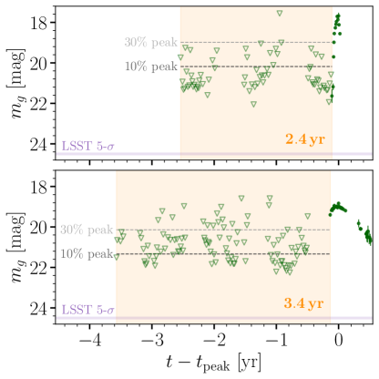
Figure 5: Forced-photometry light curves of two ZTF TDEs (ZTF20acqoiyt and ZTF21abxngcz) in $g$, where the green triangles indicate 5-$\sigma$ upper limits of 3-$\sigma$ non-detections, which have been stacked into 5-day bins to improve the signal to noise ratio. The orange shaded regions mark the span between the first ZTF observation and the first 3-$\sigma$ detection, setting the longest $P_{\mathrm{orb}}$ we could possibly constrain. Horizontal dashed lines indicate where a hypothetical pre-flare 30% (typical in our simulations) or 10% (AT 2020vdq-like) as bright as the primary flare would peak.

References

- Abramowicz & Fragile (2013) Abramowicz, M. A., & Fragile, P. C. 2013, Living Reviews in Relativity, 16, 1, doi: 10.12942/lrr-2013-1
- Andreoni et al. (2022) Andreoni, I., Coughlin, M. W., Perley, D. A., et al. 2022, Nature, 612, 430, doi: 10.1038/s41586-022-05465-8
- Antonini et al. (2011) Antonini, F., Lombardi, James C., J., & Merritt, D. 2011, ApJ, 731, 128, doi: 10.1088/0004-637X/731/2/128
- Auchettl et al. (2017) Auchettl, K., Guillochon, J., & Ramirez-Ruiz, E. 2017, ApJ, 838, 149, doi: 10.3847/1538-4357/aa633b
- Auchettl et al. (2018) Auchettl, K., Ramirez-Ruiz, E., & Guillochon, J. 2018, ApJ, 852, 37, doi: 10.3847/1538-4357/aa9b7c
- Bellm et al. (2019) Bellm, E. C., Kulkarni, S. R., Graham, M. J., et al. 2019, PASP, 131, 018002, doi: 10.1088/1538-3873/aaecbe
- Bogdanović et al. (2014) Bogdanović, T., Cheng, R. M., & Amaro-Seoane, P. 2014, ApJ, 788, 99, doi: 10.1088/0004-637X/788/2/99
- Bortolas et al. (2023) Bortolas, E., Ryu, T., Broggi, L., & Sesana, A. 2023, MNRAS, 524, 3026, doi: 10.1093/mnras/stad2024
- Broggi et al. (2024) Broggi, L., Stone, N. C., Ryu, T., et al. 2024, arXiv e-prints, arXiv:2404.05786, doi: 10.48550/arXiv.2404.05786
- Cheng & Bogdanović (2014) Cheng, R. M., & Bogdanović, T. 2014, Phys. Rev. D, 90, 064020, doi: 10.1103/PhysRevD.90.064020
- Coughlin & Nixon (2019) Coughlin, E. R., & Nixon, C. J. 2019, ApJ, 883, L17, doi: 10.3847/2041-8213/ab412d
- Cufari et al. (2022) Cufari, M., Coughlin, E. R., & Nixon, C. J. 2022, ApJ, 929, L20, doi: 10.3847/2041-8213/ac6021
- Dai et al. (2013) Dai, L., Blandford, R. D., & Eggleton, P. P. 2013, MNRAS, 434, 2940, doi: 10.1093/mnras/stt1208
- Dai et al. (2018) Dai, L., McKinney, J. C., Roth, N., Ramirez-Ruiz, E., & Miller, M. C. 2018, ApJ, 859, L20, doi: 10.3847/2041-8213/aab429
- De Colle et al. (2012) De Colle, F., Guillochon, J., Naiman, J., & Ramirez-Ruiz, E. 2012, ApJ, 760, 103, doi: 10.1088/0004-637X/760/2/103
- Dodd et al. (2021) Dodd, S. A., Law-Smith, J. A. P., Auchettl, K., Ramirez-Ruiz, E., & Foley, R. J. 2021, ApJ, 907, L21, doi: 10.3847/2041-8213/abd852
- Evans & Kochanek (1989) Evans, C. R., & Kochanek, C. S. 1989, ApJ, 346, L13, doi: 10.1086/185567
- Evans et al. (2023) Evans, P. A., Nixon, C. J., Campana, S., et al. 2023, Nature Astronomy, 7, 1368, doi: 10.1038/s41550-023-02073-y
- Faber et al. (2005) Faber, J. A., Rasio, F. A., & Willems, B. 2005, Icarus, 175, 248, doi: 10.1016/j.icarus.2004.10.021
- Falcke et al. (2004) Falcke, H., Körding, E., & Markoff, S. 2004, A&A, 414, 895, doi: 10.1051/0004-6361:20031683
- Frederick et al. (2019) Frederick, S., Gezari, S., Graham, M. J., et al. 2019, ApJ, 883, 31, doi: 10.3847/1538-4357/ab3a38
- Fryxell et al. (2000) Fryxell, B., Olson, K., Ricker, P., et al. 2000, ApJS, 131, 273, doi: 10.1086/317361
- Gafton & Rosswog (2019) Gafton, E., & Rosswog, S. 2019, MNRAS, 487, 4790, doi: 10.1093/mnras/stz1530
- Gafton et al. (2015) Gafton, E., Tejeda, E., Guillochon, J., Korobkin, O., & Rosswog, S. 2015, MNRAS, 449, 771, doi: 10.1093/mnras/stv350
- Generozov et al. (2018) Generozov, A., Stone, N. C., Metzger, B. D., & Ostriker, J. P. 2018, MNRAS, 478, 4030, doi: 10.1093/mnras/sty1262
- Gezari (2021) Gezari, S. 2021, ARA&A, 59, 21, doi: 10.1146/annurev-astro-111720-030029
- Guillochon & Ramirez-Ruiz (2013) Guillochon, J., & Ramirez-Ruiz, E. 2013, ApJ, 767, 25, doi: 10.1088/0004-637X/767/1/25
- Guillochon et al. (2011) Guillochon, J., Ramirez-Ruiz, E., & Lin, D. 2011, ApJ, 732, 74, doi: 10.1088/0004-637X/732/2/74
- Guolo et al. (2024) Guolo, M., Pasham, D. R., Zajaček, M., et al. 2024, Nature Astronomy, 8, 347, doi: 10.1038/s41550-023-02178-4
- Haas et al. (2012) Haas, R., Shcherbakov, R. V., Bode, T., & Laguna, P. 2012, ApJ, 749, 117, doi: 10.1088/0004-637X/749/2/117
- Hampel et al. (2022) Hampel, J., Komossa, S., Greiner, J., et al. 2022, Research in Astronomy and Astrophysics, 22, 055004, doi: 10.1088/1674-4527/ac5800
- Hayasaki et al. (2018) Hayasaki, K., Zhong, S., Li, S., Berczik, P., & Spurzem, R. 2018, ApJ, 855, 129, doi: 10.3847/1538-4357/aab0a5
- Hills (1975) Hills, J. G. 1975, Nature, 254, 295, doi: 10.1038/254295a0
- Hjellming & Webbink (1987) Hjellming, M. S., & Webbink, R. F. 1987, ApJ, 318, 794, doi: 10.1086/165412
- Ivanov & Novikov (2001) Ivanov, P. B., & Novikov, I. D. 2001, ApJ, 549, 467, doi: 10.1086/319050
- Jiang et al. (2016) Jiang, Y.-F., Guillochon, J., & Loeb, A. 2016, ApJ, 830, 125, doi: 10.3847/0004-637X/830/2/125
- Kıroğlu et al. (2023) Kıroğlu, F., Lombardi, J. C., Kremer, K., et al. 2023, ApJ, 948, 89, doi: 10.3847/1538-4357/acc24c
- Kremer et al. (2022) Kremer, K., Lombardi, J. C., Lu, W., Piro, A. L., & Rasio, F. A. 2022, ApJ, 933, 203, doi: 10.3847/1538-4357/ac714f
- Kumar & Goodman (1996) Kumar, P., & Goodman, J. 1996, ApJ, 466, 946, doi: 10.1086/177565
- Laguna et al. (1993) Laguna, P., Miller, W. A., Zurek, W. H., & Davies, M. B. 1993, ApJ, 410, L83, doi: 10.1086/186885
- Law-Smith et al. (2019) Law-Smith, J., Guillochon, J., & Ramirez-Ruiz, E. 2019, ApJ, 882, L25, doi: 10.3847/2041-8213/ab379a
- Law-Smith et al. (2020) Law-Smith, J. A. P., Coulter, D. A., Guillochon, J., Mockler, B., & Ramirez-Ruiz, E. 2020, ApJ, 905, 141, doi: 10.3847/1538-4357/abc489
- Lee & Ostriker (1986) Lee, H. M., & Ostriker, J. P. 1986, ApJ, 310, 176, doi: 10.1086/164674
- Li & Loeb (2013) Li, G., & Loeb, A. 2013, MNRAS, 429, 3040, doi: 10.1093/mnras/sts567
- Lin et al. (2024) Lin, Z., Jiang, N., Wang, T., et al. 2024, arXiv e-prints, arXiv:2405.10895, doi: 10.48550/arXiv.2405.10895
- Liu et al. (2023a) Liu, C., Mockler, B., Ramirez-Ruiz, E., et al. 2023a, ApJ, 944, 184, doi: 10.3847/1538-4357/acafe1
- Liu et al. (2013) Liu, S.-F., Guillochon, J., Lin, D. N. C., & Ramirez-Ruiz, E. 2013, ApJ, 762, 37, doi: 10.1088/0004-637X/762/1/37
- Liu et al. (2023b) Liu, Z., Malyali, A., Krumpe, M., et al. 2023b, A&A, 669, A75, doi: 10.1051/0004-6361/202244805
- Lodato et al. (2009) Lodato, G., King, A. R., & Pringle, J. E. 2009, MNRAS, 392, 332, doi: 10.1111/j.1365-2966.2008.14049.x
- Lu & Quataert (2023) Lu, W., & Quataert, E. 2023, MNRAS, 524, 6247, doi: 10.1093/mnras/stad2203
- MacLeod et al. (2014) MacLeod, M., Goldstein, J., Ramirez-Ruiz, E., Guillochon, J., & Samsing, J. 2014, ApJ, 794, 9, doi: 10.1088/0004-637X/794/1/9
- MacLeod et al. (2013) MacLeod, M., Ramirez-Ruiz, E., Grady, S., & Guillochon, J. 2013, ApJ, 777, 133, doi: 10.1088/0004-637X/777/2/133
- Mainetti et al. (2017a) Mainetti, D., Lupi, A., Campana, S., et al. 2017a, A&A, 600, A124, doi: 10.1051/0004-6361/201630092
- Mainetti et al. (2017b) —. 2017b, A&A, 600, A124, doi: 10.1051/0004-6361/201630092
- Malyali et al. (2023) Malyali, A., Liu, Z., Rau, A., et al. 2023, MNRAS, 520, 3549, doi: 10.1093/mnras/stad022
- Manukian et al. (2013) Manukian, H., Guillochon, J., Ramirez-Ruiz, E., & O’Leary, R. M. 2013, ApJ, 771, L28, doi: 10.1088/2041-8205/771/2/L28
- Mardling (1995a) Mardling, R. A. 1995a, ApJ, 450, 722, doi: 10.1086/176178
- Mardling (1995b) —. 1995b, ApJ, 450, 732, doi: 10.1086/176179
- Masci et al. (2019) Masci, F. J., Laher, R. R., Rusholme, B., et al. 2019, PASP, 131, 018003, doi: 10.1088/1538-3873/aae8ac
- Melchor et al. (2024) Melchor, D., Mockler, B., Naoz, S., Rose, S. C., & Ramirez-Ruiz, E. 2024, ApJ, 960, 39, doi: 10.3847/1538-4357/acfee0
- Merloni et al. (2003) Merloni, A., Heinz, S., & di Matteo, T. 2003, MNRAS, 345, 1057, doi: 10.1046/j.1365-2966.2003.07017.x
- Miles et al. (2020) Miles, P. R., Coughlin, E. R., & Nixon, C. J. 2020, ApJ, 899, 36, doi: 10.3847/1538-4357/ab9c9f
- Mockler et al. (2019) Mockler, B., Guillochon, J., & Ramirez-Ruiz, E. 2019, ApJ, 872, 151, doi: 10.3847/1538-4357/ab010f
- Mockler et al. (2023) Mockler, B., Melchor, D., Naoz, S., & Ramirez-Ruiz, E. 2023, ApJ, 959, 18, doi: 10.3847/1538-4357/ad0234
- Mockler & Ramirez-Ruiz (2021) Mockler, B., & Ramirez-Ruiz, E. 2021, ApJ, 906, 101, doi: 10.3847/1538-4357/abc955
- Narayan et al. (1998) Narayan, R., Mahadevan, R., Grindlay, J. E., Popham, R. G., & Gammie, C. 1998, ApJ, 492, 554, doi: 10.1086/305070
- Paxton et al. (2011) Paxton, B., Bildsten, L., Dotter, A., et al. 2011, ApJS, 192, 3, doi: 10.1088/0067-0049/192/1/3
- Payne et al. (2021) Payne, A. V., Shappee, B. J., Hinkle, J. T., et al. 2021, ApJ, 910, 125, doi: 10.3847/1538-4357/abe38d
- Payne et al. (2022) —. 2022, ApJ, 926, 142, doi: 10.3847/1538-4357/ac480c
- Perley et al. (2020) Perley, D. A., Fremling, C., Sollerman, J., et al. 2020, ApJ, 904, 35, doi: 10.3847/1538-4357/abbd98
- Phinney (1989) Phinney, E. S. 1989, in The Center of the Galaxy, ed. M. Morris, Vol. 136, 543
- Press & Teukolsky (1977) Press, W. H., & Teukolsky, S. A. 1977, ApJ, 213, 183, doi: 10.1086/155143
- Ramirez-Ruiz & Rosswog (2009) Ramirez-Ruiz, E., & Rosswog, S. 2009, ApJ, 697, L77, doi: 10.1088/0004-637X/697/2/L77
- Rees (1988) Rees, M. J. 1988, Nature, 333, 523, doi: 10.1038/333523a0
- Rosswog et al. (2008) Rosswog, S., Ramirez-Ruiz, E., & Hix, W. R. 2008, ApJ, 679, 1385, doi: 10.1086/528738
- Rosswog et al. (2009) —. 2009, ApJ, 695, 404, doi: 10.1088/0004-637X/695/1/404
- Ryu et al. (2020a) Ryu, T., Krolik, J., Piran, T., & Noble, S. C. 2020a, ApJ, 904, 100, doi: 10.3847/1538-4357/abb3ce
- Ryu et al. (2020b) —. 2020b, ApJ, 904, 99, doi: 10.3847/1538-4357/abb3cd
- Ryu et al. (2020c) —. 2020c, ApJ, 904, 101, doi: 10.3847/1538-4357/abb3cc
- Ryu et al. (2020d) —. 2020d, ApJ, 904, 98, doi: 10.3847/1538-4357/abb3cf
- Servin & Kesden (2017) Servin, J., & Kesden, M. 2017, Phys. Rev. D, 95, 083001, doi: 10.1103/PhysRevD.95.083001
- Soberman et al. (1997) Soberman, G. E., Phinney, E. S., & van den Heuvel, E. P. J. 1997, A&A, 327, 620, doi: 10.48550/arXiv.astro-ph/9703016
- Somalwar et al. (2023) Somalwar, J. J., Ravi, V., Yao, Y., et al. 2023, arXiv e-prints, arXiv:2310.03782, doi: 10.48550/arXiv.2310.03782
- Stone et al. (2019) Stone, N. C., Kesden, M., Cheng, R. M., & van Velzen, S. 2019, General Relativity and Gravitation, 51, 30, doi: 10.1007/s10714-019-2510-9
- Stone et al. (2020) Stone, N. C., Vasiliev, E., Kesden, M., et al. 2020, Space Sci. Rev., 216, 35, doi: 10.1007/s11214-020-00651-4
- Tejeda et al. (2017) Tejeda, E., Gafton, E., Rosswog, S., & Miller, J. C. 2017, MNRAS, 469, 4483, doi: 10.1093/mnras/stx1089
- Turk et al. (2011) Turk, M. J., Smith, B. D., Oishi, J. S., et al. 2011, ApJS, 192, 9, doi: 10.1088/0067-0049/192/1/9
- van Velzen et al. (2021) van Velzen, S., Gezari, S., Hammerstein, E., et al. 2021, ApJ, 908, 4, doi: 10.3847/1538-4357/abc258
- Wang et al. (2006) Wang, R., Wu, X.-B., & Kong, M.-Z. 2006, ApJ, 645, 890, doi: 10.1086/504401
- Weinberg et al. (2012) Weinberg, N. N., Arras, P., Quataert, E., & Burkart, J. 2012, ApJ, 751, 136, doi: 10.1088/0004-637X/751/2/136
- Wevers et al. (2019) Wevers, T., Pasham, D. R., van Velzen, S., et al. 2019, MNRAS, 488, 4816, doi: 10.1093/mnras/stz1976
- Wevers et al. (2021) —. 2021, ApJ, 912, 151, doi: 10.3847/1538-4357/abf5e2
- Wevers et al. (2023) Wevers, T., Coughlin, E. R., Pasham, D. R., et al. 2023, ApJ, 942, L33, doi: 10.3847/2041-8213/ac9f36
- Woods & Ivanova (2011) Woods, T. E., & Ivanova, N. 2011, ApJ, 739, L48, doi: 10.1088/2041-8205/739/2/L48
- Yao et al. (2023) Yao, Y., Ravi, V., Gezari, S., et al. 2023, ApJ, 955, L6, doi: 10.3847/2041-8213/acf216