An efficient Wasserstein-distance approach for reconstructing jump-diffusion processes using parameterized neural networks

Mingtao Xia1111corresponding author, Xiangting Li2, Qijing Shen3, Tom Chou4 1 Courant Institute of Mathematical Sciences, New York University, New York, NY 10012, USA
2 Department of Computational Medicine, UCLA, Los Angeles, CA 90095, USA
3 Nuffield Department of Medicine, University of Oxford, Oxford OX2 6HW, UK
4 Department of Mathematics, UCLA, Los Angeles, CA 90095, USA
xiamingtao@nyu.edu, xiangting.li@ucla.edu,qijing.shen@ndm.ox.ac.uk, tomchou@ucla.edu
(July 6, 2024)
Abstract

We analyze the Wasserstein distance ($W$-distance) between two probability distributions associated with two multidimensional jump-diffusion processes. Specifically, we analyze a temporally decoupled squared $W_{2}$-distance, which provides both upper and lower bounds associated with the discrepancies in the drift, diffusion, and jump amplitude functions between the two jump-diffusion processes. Then, we propose a temporally decoupled squared $W_{2}$-distance method for efficiently reconstructing unknown jump-diffusion processes from data using parameterized neural networks. We further show its performance can be enhanced by utilizing prior information on the drift function of the jump-diffusion process. The effectiveness of our proposed reconstruction method is demonstrated across several examples and applications.

Keywords: Jump-diffusion process, Inverse problem, Wasserstein distance, Neural Network

1 Introduction

Jump-diffusion processes are widely used across many disciplines such as finance [1, 2, 3], biology [4], epidemiology [5], and so on. A $d$-dimensional jump-diffusion process may be written in the following form [6]:

$$\text{d}\bm{X}(t)=\bm{f}(\bm{X}(t),t)\text{d}t+\bm{\sigma}(\bm{X}(t),t)\text{d}\bm{B}_{t}+\int_{U}\bm{\beta}(\bm{X}(t),\xi,t)\tilde{N}(\text{d}t,\nu(\text{d}\xi))$$ (1)

Here, $\bm{X}(t)\in\mathbb{R}^{d}$ is a $d$-dimensional jump-diffusion process and $\bm{B}_{t}\coloneqq(B_{1,t},...,B_{m,t})$ is a standard $m$-dimensional white noise; $\tilde{N}$ is a compensated Poisson process of intensity $\nu(\text{d}\xi)\text{d}t$ independent of $\bm{B}_{t}$:

$$\tilde{N}(\text{d}t,\nu(\text{d}\xi))\coloneqq N(\nu(\text{d}\xi),\text{d}t)-\nu(\text{d}\xi)\text{d}t,$$ (2)

where $N(\nu(\text{d}\xi),\text{d}t)$ is a Poisson process with intensity $\nu(\text{d}\xi)\text{d}t$ and $\nu(\text{d}\xi)$ is a measure defined on $U\subseteq\mathbb{R}$, the measure space of the Poisson process. $N(A,B)$ and $N(C,D)$ are independent if $(A\times B)\cap(C\times D)=\emptyset,A,C\subseteq\mathcal{B}(U)$ and $B,D\subseteq\mathcal{B}([0,T])$. $\mathcal{B}(U)$ and $\mathcal{B}([0,T])$ denote the $\sigma$-algebra associated with $U$ and $[0,T]$, respectively. The drift, diffusion, and jump functions are defined by

$\displaystyle\bm{f}\coloneqq$ $\displaystyle\big{(}f_{1}(\bm{X},t),...,f_{d}(\bm{X},t)\big{)}\in C(\mathbb{R}^{d}\times[0,T],\mathbb{R}^{d}),$ (3)
$\displaystyle\bm{\sigma}\coloneqq$ $\displaystyle\big{(}\sigma_{i,j}(\bm{X},t)\big{)}\in C(\mathbb{R}^{d}\times[0,T],\mathbb{R}^{d\times m}),$
$\displaystyle\bm{\beta}\coloneqq$ $\displaystyle\big{(}\beta_{i}(\bm{X},\xi,t)\big{)}\in C(\mathbb{R}^{d}\times U\times[0,T],\mathbb{R}^{d}),$

respectively. Specifically, if $U=\{1,...,n\}$, then Eq. (1) becomes

$$\text{d}X_{i}(t)=f_{i}(\bm{X}(t),t)\text{d}t+\sum_{j=1}^{m}\sigma_{i,j}(\bm{X}(t),t)\text{d}(B_{j})_{t}+\sum_{s=1}^{n}\beta_{i,s}(\bm{X}(t),s,t)\tilde{N}_{s}(\text{d}t,\nu(s))$$ (4)

for $i=1,..,d$. Here, each $\tilde{N}_{s}$ is a compensated Poisson process with intensity $\nu(s)\text{d}t$. $\tilde{N}_{s_{1}}$ and $\tilde{N}_{s_{2}}$ are independent if $s_{1}\neq s_{2}$. When $\bm{\beta}\equiv 0$, Eq. (1) reduces to the pure diffusion process.

In this paper, we study the problem of reconstructing a jump-diffusion process Eq. (1) or Eq. (4) from observed data $\bm{X}(t)$ at different time points by using a different jump-diffusion process

$\displaystyle\text{d}\hat{\bm{X}}(t)=\hat{\bm{f}}(\bm{X}(t),t)\text{d}t+\hat{\bm{\sigma}}(\hat{\bm{X}}(t),t)\text{d}\hat{\bm{B}}_{t}+\!\int_{U}\hat{\bm{\beta}}(\hat{\bm{X}}(t),\xi,t)\hat{N}\big{(}\text{d}t,\nu(\text{d}\xi)\big{)}$ (5)

to approximate Eq. (1). In Eq. (5), $\hat{\bm{B}}_{t}$ is a $m$-dimensional standard Brownian motion that is independent of $\bm{B}_{t}$ and $\tilde{N}$ in Eq. (1); $\hat{N}(\text{d}t,\nu(\text{d}\xi))$ is a compensated Poisson process of intensity $\text{d}\nu(\xi)\text{d}t$ and independent of $\bm{B}_{t}$, $\tilde{N}$ in Eq. (1) as well as $\hat{\bm{B}}_{t}$. Specifically, we are interested in reconstructing the jump-diffusion process Eq. (1) with little or no prior information on the drift, diffusion, and jump functions $\bm{f},\bm{\sigma}$, and $\bm{\beta}$. To reconstruct or approximate Eq. (1) using Eq. (5), we wish to find small errors in the drift, diffusion, and jump functions, i.e., to find $\hat{\bm{f}},\hat{\bm{\sigma}}$, and $\hat{\bm{\beta}}$ such that $\bm{f}-\hat{\bm{f}}$, $\bm{\sigma}-\hat{\bm{\sigma}}$, and $\bm{\beta}-\hat{\bm{\beta}}$ are small.

Thus far, most studies related to jump-diffusion processes have focused on the forward-type problem of efficient simulation of a jump-diffusion process given coefficients [7, 8]. There are also several studies on the statistical properties of jump-diffusion processes such as their first passage times [9, 10]. While there has been some research into the inverse problem of reconstructing a general pure diffusion process, there has been little work on reconstructing unknown jump-diffusion processes from sample trajectories although two main strategies have been proposed. First, regression methods are applied to determine unknown parameters if the forms of drift, diffusion, and jump functions ($\bm{f}$, $\bm{\sigma}$ and $\bm{\beta}$ in Eq. (1)) are known. Unknown parameters in these functions can then be determined from data [11, 12]. Another strategy for reconstructing a jump-diffusion process is to calculate the empirical probability density function $p(\bm{X},t)$ from observation data $\bm{X}(t)$ and then reconstruct the integrodifferential equation satisfied by $p(\bm{X},t)$ [13]. Yet, this method requires a large number of observations at different time points to obtain a good empirical approximation of the density function $p(\bm{X},t)$. Recently, a Wasserstein-generative-adversarial-network(WGAN)-based method was proposed to reconstruct the jump-diffusion process Eq. (1) [4]. However, training a WGAN can be intricate and computationally expensive.

Recent advancements in machine learning make it possible to use parameterized neural networks (NNs) for representing $\hat{\bm{f}},\hat{\bm{\sigma}}$, and $\hat{\bm{\beta}}$ in Eq. (5) which approximate $\bm{f},\bm{\sigma}$, and $\bm{\beta}$ in Eq. (1). For example, a recent torchsde package in Python [14] models pure diffusion processes (SDEs with Brownian noise) by using parameterized neural networks. These methods have been used in the reconstruction of diffusion processes. For example, in [15], a deep Gaussian latent model has been applied for reconstructing a pure diffusion process; [16] uses the neural SDE model to reconstruct a stochastic differential equation with Brownian noise by minimizing a KL-divergence-based loss function. In [17, 18], generative adversarial networks were used to reconstruct general stochastic differential equations including a Brownian motion noise term without requiring prior knowledge of the specific forms of the drift or diffusion functions.

Another recent work analyzes the upper bound for a smooth Wasserstein distance between two distributions associated with two 1D jump-diffusion processes at a given time [19]. Since the $W$-distance can effectively measure discrepancies between probability measures over a metric space [20, 21], an efficient squared-Wasserstein-distance-based method for reconstructing pure diffusion processes from data, without the need to specify forms for the drift and diffusion, was recently proposed [22]. General jump-diffusion processes are distinct from pure diffusion processes because the trajectories of jump-diffusion processes are discontinuous. Thus, it remains unclear whether the Wasserstein distance can also be employed to reconstruct an unknown jump-diffusion process from data.

1.1 Contribution

In this paper, we analyze the $W$-distance between two probability distributions associated with two multidimensional jump-diffusion processes Eqs. (1) and  (5). We then show that a temporally decoupled squared Wasserstein distance can serve as effective upper and lower error bounds on the errors in the drift, diffusion, and jump functions $\bm{f}-\hat{\bm{f}}$, $\bm{\sigma}-\hat{\bm{\sigma}}$, and $\bm{\beta}-\hat{\bm{\beta}}$ in Eqs. (1) and (5), respectively. This temporally decoupled squared Wasserstein distance can be effectively evaluated using finite-sample observations at discrete time points. Thus, we propose using this temporally decoupled squared $W_{2}$-distance to reconstruct general jump-diffusion processes with the help of parameterized neural networks. Furthermore, we explore how prior information on the drift function enhances the performance of our temporally decoupled squared Wasserstein distance method. Our results greatly extend the results in [22] (reconstructing 1D pure diffusion processes) to allow for the reconstruction of multidimensional jump-diffusion processes. Specifically, we

  1. 1.

    prove that the $W$-distance is a lower bound for the errors $\bm{f}-\hat{\bm{f}},\bm{\sigma}-\hat{\bm{\sigma}}$, and $\bm{\beta}-\hat{\bm{\beta}}$. Thus, minimizing the $W$-distance is necessary for reconstructing the multidimensional jump-diffusion process Eq. (1).

  2. 2.

    analyze a temporally decoupled squared $W$-distance defined in [22] and show that it can be efficiently evaluated by finite-sample empirical distributions. Thus, it is suitable to serve as a loss function to minimize for reconstructing Eq. (1) using parameterized neural networks.

  3. 3.

    conduct numerical experiments to demonstrate the efficacy of using the temporally decoupled squared Wasserstein distance to reconstruct jump-diffusion processes. Our temporally decoupled squared Wasserstein method performs better than some other benchmark methods. Additionally, we propose incorporating prior information on the drift function, which greatly improves the accuracy of reconstructed diffusion and jump functions.

1.2 Organization

In Section 2, we analyze how the $W$-distance between the probability measures associated with solutions to two jump-diffusion processes Eqs. (1) and (5) can be a lower bound of the errors in the reconstructed drift, diffusion, and jump functions $\bm{f}-\hat{\bm{f}}$, $\bm{\sigma}-\hat{\bm{\sigma}}$, and $\bm{\beta}-\hat{\bm{\beta}}$. In Section 3, we analyze a temporally decoupled squared $W_{2}$-distance and show how it can be more effectively evaluated than the squared $W_{2}$ distance. Specifically, the temporally decoupled squared $W_{2}$ distance is smaller than the $W_{2}$ distance analyzed in Section 2 while providing an upper bound of the errors in the reconstructed drift, diffusion, and jump functions. Thus, Sections 2 and  3 together show that our temporally decoupled squared $W_{2}$ distance provides both upper and lower error bounds. In Section 4, numerical experiments are carried out to compare our proposed jump-diffusion process reconstruction methods with other methods for reconstructing different jump-diffusion processes. Additionally, we show how prior information on the drift function of the ground truth jump-diffusion process Eq. (1) improves the reconstruction of the diffusion and jump functions in Eq. (1). In Section 5, we summarize our proposed jump-diffusion process reconstruction approach and suggest potential future directions.

2 The $W$-distance between the probability measures associated with the jump-diffusion processes in Eqs. (1) and (5)

In this section, we shall show how the $W$-distance between the probability measures associated with the two jump-diffusion processes Eqs. (1) and (5) can serve as a lower bound for the errors $\bm{f}-\hat{\bm{f}}$, $\bm{\sigma}-\hat{\bm{\sigma}}$, and $\bm{\beta}-\hat{\bm{\beta}}$. First, we specify the assumptions on the jump-diffusion processes in Eqs. (1) and (5).

Assumption 2.1.

We assume that the jump-diffusion processes defined in Eq. (1) satisfy the following conditions:

  1. 1.

    For each non-increasing sequence $A_{i}\subseteq U$ converging to the empty set $\emptyset$, $\mathbb{E}\big{[}|\tilde{N}(t,A)|^{2}\big{]}\rightarrow 0,\forall t\geq 0$.

  2. 2.

    $\tilde{N}(t,A)$ is a càdlàg martingale for all $A\subseteq U,t>0$, and $\mathbb{E}[|\tilde{N}(t,U)|^{2}]<\infty$.

  3. 3.

    $\tilde{N}\big{(}\text{d}t,\nu(\text{d}\xi)\big{)}$ is an orthogonal martingale measure with intensity $\text{d}t\cdot\nu(\text{d}\xi)$, i.e., for any $A,B\subseteq U$ and $t_{1}<t_{2},t_{3}\leq t_{4}$ and any $\beta_{1}(\xi,t),\beta_{2}(\xi,t)\in L^{2}([0,T]\times U)$ (the measure on $U$ is $\nu$), we have

    $\displaystyle\mathbb{E}\bigg{[}\!\medint\int_{t_{1}}^{t_{2}}\!\!\!\medint\int_{A}\beta_{1}(\xi,t)\tilde{N}\big{(}\text{d}t,\nu(\text{d}\xi)\big{)}\medint\int_{t_{3}}^{t_{4}}\!\!\!\medint\int_{B}\beta_{2}(\xi,t)\tilde{N}\big{(}\text{d}t,\nu(\text{d}\xi)\big{)}\bigg{]}=\!\!\!\!\!\medint\int\limits_{[t_{1},t_{2}]\cap[t_{3},t_{4}]}\!\!\!\!\medint\int_{A\cap B}\beta_{1}(\xi,t)\beta_{2}(\xi,t)\nu(\text{d}\xi)\text{d}{t}.$ (6)
  4. 4.

    Trajectories generated from both jump-diffusion processes, Eqs. (1) and (5), reside in the space $L^{2}([0,T],\mathbb{R}^{d})$.

  5. 5.

    The drift, diffusion, and jump functions are all uniformly Lipschtiz continuous, i.e., there exists three positive constants $\overline{f},\overline{\sigma},\overline{\beta}<\infty$ such that $\forall\bm{X}^{1}=(X^{1}_{1},...,X^{1}_{d}),\forall\bm{X}^{2}=(X^{2}_{1},...,X^{2}_{d})\in\mathbb{R}^{d}$,

    $\displaystyle\big{|}f_{i}(\bm{X}^{1},t)-f_{i}(\bm{X}^{2},t)\big{|}$ $\displaystyle\leq\frac{\overline{f}}{d}\sum_{i=1}^{d}\big{|}X_{i}^{1}-X_{i}^{2}\big{|},\,\,\,\forall i=1,...,d$ (7)
    $\displaystyle\big{|}\sigma_{i,j}(\bm{X}^{1},t)-\sigma_{i,j}(\bm{X}^{2},t)\big{|}$ $\displaystyle\leq\frac{\overline{\sigma}}{d}\sum_{i=1}^{d}\big{|}X_{i}^{1}-X_{i}^{2}\big{|},\,\,\forall i=1,...,d,\,\,\forall j=1,...,m,$
    $\displaystyle\big{|}\beta_{i}(\bm{X}^{1},\xi,t)-\beta_{i}(\bm{X}^{2},\xi,t)\big{|}$ $\displaystyle\leq\frac{\overline{\beta}}{d}\sum_{i=1}^{d}\big{|}X_{i}^{1}-X_{i}^{2}\big{|},\,\,\,\forall i=1,...,d.$

Furthermore, we assume that conditions (i)-(iv) also hold for the compensated Poisson process $\hat{N}$ in Eq. (5), and that condition (v) holds for the drift, diffusion, and jump functions in Eq. (5).

Now consider the $W$-distance between the distributions associated with solutions generated from the target jump-diffusion process Eq. (1) and the approximate jump-diffusion process Eq. (5), as defined below.

Definition 2.1.

For two $d$-dimensional jump-diffusion processes

$$\bm{X}(t)=(X_{1}(t),...,X_{d}(t)),\,\,\,\hat{\bm{X}}(t)=(\hat{{X}}_{1}(t),...,\hat{X}_{d}(t)),\,\,t\in[0,T],$$ (8)

in the separable space $\big{(}L^{2}([0,T];\mathbb{R}^{d}),\|\cdot\|\big{)}$ with two associated probability distributions $\mu,\hat{\mu}$, respectively, the $W_{p}$-distance $W_{p}(\mu,\hat{\mu})$ for $1\leq p\leq 2$ is defined as

$$W_{p}(\mu,\hat{\mu})\coloneqq\inf_{\pi(\mu,\hat{\mu})}\mathbb{E}_{(\bm{X},\hat{\bm{X}})\sim\pi(\mu,\hat{\mu})}\big{[}\|{\bm{X}}-\hat{{\bm{X}}}\|^{p}\big{]}^{\frac{1}{p}}.$$ (9)

In Eq. (9), the norm $\|\cdot\|$ is defined as $\|\bm{X}\|\coloneqq\Big{(}\int_{0}^{T}\sum_{i=1}^{d}|X_{i}(t)|^{2}\text{d}t\Big{)}^{\frac{1}{2}}$ and $\pi(\mu,\hat{\mu})$ iterates over all coupled distributions of $\bm{X}(t),\hat{\bm{X}}(t)$, defined by the condition

$$\begin{cases}{\bm{P}}_{\pi(\mu,\hat{\mu})}\left(A\times L^{2}([0,T];\mathbb{R}^{d})\right)={\bm{P}}_{\mu}(A),\\ {\bm{P}}_{\pi(\mu,\hat{\mu})}\left(L^{2}([0,T];\mathbb{R}^{d})\times A\right)={\bm{P}}_{\hat{\mu}}(A),\end{cases}\forall A\in\mathcal{B}\Big{(}L^{2}([0,T];\mathbb{R}^{d})\Big{)},$$ (10)

where $\mathcal{B}\Big{(}L^{2}([0,T];\mathbb{R}^{d})\Big{)}$ denotes the Borel $\sigma$-algebra associated with the space of $d$-dimensional functions in $L^{2}([0,T];\mathbb{R}^{d})$.

To prove that $W_{p}(\mu,\hat{\mu})$ defined in Eq. (9) is a lower bound for the errors in the drift, diffusion, and jump functions $\bm{f}-\hat{\bm{f}}$, $\bm{\sigma}-\hat{\bm{\sigma}}$, and $\bm{\beta}-\hat{\bm{\beta}}$, we first prove the following theorem.

Theorem 2.1.

Suppose $\bm{X}(t)$ and $\hat{\bm{X}}(t)$ are two $d$-dimensional jump-diffusion processes that are determined by Eq. (1) and Eq. (5). We denote

$$\text{d}\tilde{\bm{X}}(t)=\hat{\bm{f}}\big{(}\tilde{\bm{X}}(t),t\big{)}+\hat{\bm{\sigma}}\big{(}\tilde{\bm{X}}(t),t\big{)}\text{d}\bm{B}_{t}+\!\int_{U}\hat{\bm{\beta}}\big{(}\tilde{\bm{X}}(t),\xi,t\big{)}\tilde{N}\big{(}\text{d}t,\nu(\text{d}\xi)\big{)}$$ (11)

and assume that

$$\int_{0}^{t}\big{(}X_{i}(s^{-})-\tilde{X}_{i}(s^{-})\big{)}\big{(}\sigma_{i,j}-\hat{\sigma}_{i,j}\big{)}\text{d}B_{j,t},\,\,\,\int_{0}^{t}\!\int_{U}\big{(}X_{i}(s^{-})-\tilde{X}_{i}(s^{-})\big{)}\big{(}\beta_{i}-\hat{\beta}_{i}\big{)}\text{d}\tilde{N}\big{(}\text{d}t,\nu(\text{d}\xi)\big{)},$$ (12)

are martingales for all $i,j$. Then, the following inequality holds:

$$\mathbb{E}\Big{[}\big{|}\bm{X}(t)-\tilde{\bm{X}}(t)\big{|}_{2}^{2}\Big{]}\leq\mathbb{E}\big{[}H(T)|\bm{X}(0)\big{]}\exp\Big{(}\big{(}2\overline{f}+1+(2\overline{\sigma}+1)m+(2\overline{\beta}+1)\nu(U)\big{)}T\Big{)},$$ (13)

where $|\cdot|_{2}$ denotes the $2$-norm of a $d$-dimensional vector, $\bm{X}(0)$ is the initial condition, and $H(t)$ is defined as

$\displaystyle H(t)\coloneqq$ $\displaystyle\mathbb{E}\bigg{[}\sum_{i=1}^{d}\int_{0}^{t}\big{(}f_{i}(\bm{X}(s^{-}),s^{-})-\hat{f}_{i}(\bm{X}(s^{-}),s^{-})\big{)}^{2}\text{d}s\bigg{]}$ (14)
$\displaystyle\quad+\mathbb{E}\bigg{[}\sum_{i=1}^{d}\int_{0}^{t}\sum_{j=1}^{m}\big{(}\sigma_{i,j}(\bm{X}(s^{-}),s^{-})-\hat{\sigma}_{i,j}(\bm{X}(s^{-}),s^{-})\big{)}^{2}\text{d}s\bigg{]}$
$\displaystyle\qquad+\mathbb{E}\bigg{[}\sum_{i=1}^{d}\int_{0}^{t}\int_{U}\big{(}\beta_{i}(\bm{X}(s^{-}),\xi,s^{-})-\hat{\beta}_{i}(\bm{X}(s^{-}),\xi,s^{-})\big{)}^{2}\nu(\text{d}\xi)\text{d}s\bigg{]}$

The proof to Theorem 2.1 is similar to the proof of the stochastic Gronwall lemma (Theorem 2.2 in [6]) and is given in A. Theorem 2.1 greatly generalizes the results of Theorem 1 in [22], which was developed for analyzing the $W_{2}$-distance between two one-dimensional pure diffusion processes. Now, with Theorem 2.1, we can analyze the $W$-distance between two multi-dimensional jump-diffusion processes.

The following corollary establishes the upper bound of the $W$-distance $W_{p}(\mu,\hat{\mu}),1\leq p\leq 2$ between $\mu$ and $\hat{\mu}$, the two probability distributions associated with jump-diffusion processes Eqs. (1) and  (5).

Corollary 2.1.

(Upper error bound for the $W$-distance) The following bound holds for $W_{p}(\mu,\hat{\mu})$, where $\mu$ and $\hat{\mu}$ are the two probability distributions associated with jump-diffusion processes Eqs. (1) and  (5)

$$W_{p}(\mu,\hat{\mu})\leq\sqrt{\,T\mathbb{E}\big{[}H(T)\big{|}\bm{X}(0)\big{]}}\times\exp\Big{(}\big{(}\overline{f}+\tfrac{1}{2}+(\overline{\sigma}+\tfrac{1}{2})m+(\overline{\beta}+\tfrac{1}{2})\nu(U)\big{)}T\Big{)},$$ (15)

where $H(T)$ is defined in Eq. (14).

Proof.

The proof of Corollary 2.1 is a direct application of Theorem 2.1. We denote $\tilde{\mu}$ to be the distribution of $\tilde{\bm{X}}$ defined in Eq. (11). Since $\tilde{\bm{X}}$ has the same distribution as $\hat{\bm{X}}$, we have, by the Hölder’s inequality

$$W_{p}^{p}(\mu,\hat{\mu})=W_{p}^{p}(\mu,\tilde{\mu})\leq\mathbb{E}\bigg{[}\!\int_{0}^{T}\!\big{|}\bm{X}(s)-\tilde{\bm{X}}(s)\big{|}_{2}^{2}\text{d}s\,\Big{|}\,\bm{X}(0)\bigg{]}^{\frac{p}{2}},\,\,\,1\leq p\leq 2.$$ (16)

Using Eq. (13) and the fact that $H(t)$ is non-decreasing w.r.t. $t$, we have

$$W_{p}(\mu,\hat{\mu})\leq\sqrt{\,T\mathbb{E}\big{[}H(T)\big{|}\bm{X}(0)\big{]}}\times\exp\Big{(}\big{(}(\overline{f}+\tfrac{1}{2})+(\overline{\sigma}+\tfrac{1}{2})m+(\overline{\beta}+\tfrac{1}{2})\nu(E)\big{)}T\Big{)},\,\,\,1\leq p\leq 2.$$ (17)

which proves Eq. (15).

From Corollary 2.1, it is necessary to have a small $W_{p}(\mu,\hat{\mu})$ in Eq. (15) such that the errors in the drift, diffusion, and jump functions $\bm{f}-\hat{\bm{f}}$, $\bm{\sigma}-\hat{\bm{\sigma}}$, and $\bm{\beta}-\hat{\bm{\beta}}$ can be small. Note that Corollary 2.1 analyzes the classic $W_{p}$-distance $W_{p}(\mu,\hat{\mu})$, which is different from the smooth Wasserstein distance in [19] (the classical Wasserstein distance is an upper bound for the smooth Wasserstein distance used in [23]).

$W_{p}(\mu,\hat{\mu}),1\leq p\leq 2$ cannot be directly used as a loss function to minimize as we cannot directly evaluate $\|\bm{X}-\hat{\bm{X}}\|^{p}$ in Eq. (9) since this term requires evaluation of the integral $\int_{0}^{T}\sum_{i=1}^{d}|X_{i}(t)-\hat{X}_{i}(t)|^{2}\text{d}t$. However, when $p=2$ ($W_{2}(\mu,\hat{\mu})$), we shall show that we can efficiently estimate $W_{2}(\mu,\hat{\mu})$ by using finite-time-point observations of the two jump-diffusion processes $\bm{X}(t)$ and $\hat{\bm{X}}(t)$.

Let $0=t_{0}<t_{1}<...<t_{N}=T$ to be a mesh grid in the time interval $[0,T]$, and we define the following projection operator $I_{N}$

$$\bm{X}_{N}(t)\coloneqq I_{N}\bm{X}(t)=\begin{cases}&\bm{X}(t_{i}),t\in[t_{i},t_{i+1}),\quad i<N-1,\\ &\bm{X}(t_{i}),t\in[t_{i},t_{i+1}],\quad i=N-1.\end{cases}$$ (18)

The projected $\bm{X}_{N}(t)$ in Eq. (18) is piecewise constant and is thus in the space $L^{2}([0,T])$. We denote the distributions of $\bm{X}_{N}(t)$ and $\hat{\bm{X}}_{N}(t)\coloneqq I_{N}\hat{\bm{X}}_{N}$ in Eq. 18 by $\mu_{N}$ and $\hat{\mu}_{N}$, respectively. We will prove the following theorem for bounding the error $|W_{2}(\mu,\hat{\mu})-W_{2}\left(\mu_{N},\hat{\mu}_{N}\right)|$.

Theorem 2.2.

(Finite-time-point approximation for $W_{2}$ distance) The following triangular inequality for $W_{2}(\mu,\hat{\mu})$ holds:

$\displaystyle W_{2}(\mu_{N},\hat{\mu}_{N})-W_{2}(\mu,\mu_{N})-W_{2}(\hat{\mu},\hat{\mu}_{N})\leq W_{2}(\mu,\hat{\mu})\leq W_{2}(\mu_{N},\hat{\mu}_{N})+W_{2}(\mu,\mu_{N})+W_{2}(\hat{\mu},\hat{\mu}_{N}).$ (19)

In Eq. (19), $\mu_{N},\hat{\mu}_{N}$ are the probability distributions associated with $\bm{X}_{N}$ and $\hat{\bm{X}}_{N}$ defined in Eq. (18), respectively. Furthermore, we assume that

$\displaystyle F\coloneqq$ $\displaystyle\mathbb{E}\Big{[}\medint\int_{0}^{T}{\small\sum}_{i=1}^{d}f_{i}^{2}(\bm{X}(t^{-}),t^{-})\text{d}t\Big{]}<\infty,$ $\displaystyle\hat{F}\coloneqq\mathbb{E}\Big{[}\medint\int_{0}^{T}\sum_{i=1}^{d}\hat{f}_{i}^{2}(\hat{\bm{X}}(t^{-}),t^{-})\text{d}t\Big{]}<\infty$ (20)
$\displaystyle\Sigma\coloneqq$ $\displaystyle\mathbb{E}\Big{[}\medint\int_{0}^{T}\sum_{\ell=1}^{d}\sum_{j=1}^{m}\sigma_{i,j}^{2}(\bm{X}(t^{-}),t^{-})\text{d}t\Big{]}<\infty,$ $\displaystyle\hat{\Sigma}\coloneqq\mathbb{E}\Big{[}\medint\int_{0}^{T}\sum_{\ell=1}^{d}\sum_{j=1}^{m}\hat{\sigma}_{i,j}^{2}(\hat{\bm{X}}(t^{-}),t^{-})\text{d}t\Big{]}<\infty,$
$\displaystyle B\coloneqq$ $\displaystyle\mathbb{E}\Big{[}\medint\int_{0}^{T}\sum_{\ell=1}^{d}\medint\int_{U}\beta_{i}^{2}(\bm{X}(t^{-}),\xi,t^{-})\nu(\text{d}\xi)\text{d}t\Big{]}<\infty,$ $\displaystyle\hat{B}\coloneqq\mathbb{E}\Big{[}\medint\int_{0}^{T}\sum_{\ell=1}^{d}\medint\int_{U}\hat{\beta}_{i}^{2}(\hat{\bm{X}}(t^{-}),\xi,t^{-})\nu(\text{d}\xi)\text{d}t\Big{]}<\infty,$

where $\bm{X}(t)$ and $\hat{\bm{X}(t)}$ solve Eqs. (1) and (5), respectively. Then, we have the following bound

$$\big{|}W_{2}(\mu_{N},\hat{\mu}_{N})-W_{2}(\mu,\hat{\mu})\big{|}\leq\sqrt{\Delta t}\left(\sqrt{F\Delta t+\Sigma+B}+\sqrt{\hat{F}\Delta t+\hat{\Sigma}+\hat{B}}\right).$$ (21)

where $\Delta t\coloneqq\max_{i=0,...,N-1}|t_{i+1}-t_{i}|$.

The proof to Theorem 2.2, given in  B, uses the Itô isometry as well as the orthogonal assumption of the compensated Poisson process in Assumption 2.1. Theorem 2.2 indicates that $W_{2}(\mu,\hat{\mu})$ can be approximated by the finite-time-point projections $\bm{X}_{N}$ and $\hat{\bm{X}}_{N}$. Specifically, Theorem 2.2 is a generalization to Theorem 2 in [22], developed for the pure diffusion. Note that Eq. (21) holds for $|W_{2}(\mu,\hat{\mu})-W_{2}(\mu_{N},\hat{\mu}_{N})|$ but Eq. (21) might not hold for $|W_{p}(\mu,\hat{\mu})-W_{p}(\mu_{N},\hat{\mu}_{N})|,\,1\leq p<2$ as we cannot directly apply the Itô isometry to the compensated Poisson process for $1\leq p<2$.

It has been shown in [22] that for reconstructing pure diffusion processes, minimizing a temporally decoupled squared $W_{2}$ distance can yield more accurate reconstructions of the drift and diffusion functions than direct minimization of the squared $W_{2}$ distance $W_{2}^{2}(\mu,\hat{\mu})$ defined in Eq. (9). Additionally, the squared $W_{2}$ distance $W_{2}(\mu,\hat{\mu})$ is an upper bound of the temporally decoupled squared $W_{2}$ distance that will be discussed in Section 3. Thus, Corollary 2.1 also applies to the temporally decoupled squared $W_{2}$ distance.

3 A temporally decoupled squared $W_{2}$ distance

In this section, we propose and analyze a temporally decoupled squared $W_{2}$ distance, which could help effectively approximate the jump-diffusion process Eq. (1) by the reconstructed jump-diffusion process Eq. (5). Specifically, we show why this temporally decoupled squared $W_{2}$ distance can be more effectively evaluated using empirical distributions, making it a more appealing choice than the squared $W_{2}$ distance $W_{2}^{2}(\mu,\hat{\mu})$ discussed in Section 2. The temporally decoupled squared $\bm{W_{2}}$ distance is defined as

$$\tilde{W}_{2}^{2}(\mu,\hat{\mu})\coloneqq\int_{0}^{T}\!W_{2}^{2}\big{(}\mu(t),\hat{\mu}(t)\big{)}\text{d}t,$$ (22)

where $\mu(t),\hat{\mu}(t)$ are the distributions of $d$-dimensional random variables $\bm{X}(t)$ and $\bm{X}(t)$ at time $t$, respectively:

$$W_{2}^{2}(\mu(t),\hat{\mu}(t))\coloneqq\!\inf_{\pi(\mu(t),\hat{\mu}(t))}\!\mathbb{E}_{(\bm{X}(t),\hat{\bm{X}(t)})\sim\pi(\mu,\hat{\mu})}\big{[}|{\bm{X}}(t)-\hat{{\bm{X}}}(t)|_{2}^{2}\big{]},$$ (23)

where the joint distribution $\pi(\mu(t),\hat{\mu}(t))$ satisfies

$$\pi(\mu(t),\hat{\mu}(t))(A,\mathbb{R}^{d})=\mu(t)(A),\,\,\,\,\pi(\mu(t),\hat{\mu}(t))(\mathbb{R}^{d},B)=\hat{\mu}(t)(B),\,\,\,\,A,B\in\mathcal{B}(\mathbb{R}^{d}).$$ (24)

The integration on the RHS of Eq. (22) is defined as the limit

$$\int_{0}^{T}\!W_{2}^{2}(\mu(t),\hat{\mu}(t))\text{d}t=\lim\limits_{\max_{i}(t_{i+1}-t_{i})\rightarrow 0}\sum_{i=0}^{N-1}W_{2}^{2}(\mu(t_{i}),\hat{\mu}(t_{i}))\Delta t_{i},$$ (25)

where $0=t_{0}<t_{1}<...<t_{N}=T$ is a grid mesh on the time interval $[0,T]$ and $\Delta t_{i}\coloneqq t_{i+1}-t_{i}$ in the following. Here, we shall prove that the temporally decoupled squared $W_{2}$ distance $\tilde{W}_{2}^{2}(\mu,\hat{\mu})$ is well defined and can be a more effective loss function when seeking to reconstruct multidimensional jump-diffusion processes than the original squared $W_{2}^{2}(\mu_{N},\hat{\mu}_{N})$. Two features make this so: i) numerically evaluating the temporally decoupled squared $W_{2}$ distance Eq. (22) using finite-sample empirical distributions can be more accurate than evaluating the original squared $W_{2}$ distance $W_{2}^{2}(\mu,\hat{\mu})$ when the number of training samples becomes larger, and ii) the temporally decoupled squared $W_{2}$ distance Eq. (22) provides upper error bounds for $\bm{f}-\hat{\bm{f}},\bm{\sigma}-\hat{\bm{\sigma}}$, and $\bm{\beta}-\hat{\bm{\beta}}$ when reconstructing jump-diffusion processes.

We denote $\bm{\mu}_{i}$ and $\hat{\bm{\mu}}_{i}$ to be the distributions for $\bm{X}(t),t\in[t_{i},t_{i+1})$ and $\hat{\bm{X}}(t),t\in[t_{i},t_{i+1})$, respectively. We can prove the following theorem that shows the limit on the RHS of Eq. (25) exists and thus the temporally decoupled squared $W_{2}$ in Eq. (22) distance is well defined.

Theorem 3.1.

(The temporally decoupled squared $W_{2}$ distance is well-defined) We assume the conditions in Theorem 2.2 hold. Furthermore, we assume that for any $0<t<t^{\prime}<T$, as $t^{\prime}-t\rightarrow 0$, the following conditions are satisfied

$\displaystyle\mathbb{E}\bigg{[}\medint\int_{t}^{t^{\prime}}\!\sum_{i=1}^{d}f_{i}^{2}(\bm{X}(t),t)\text{d}t\bigg{]}\rightarrow 0,$ $\displaystyle\mathbb{E}\bigg{[}\medint\int_{t}^{t^{\prime}}\sum_{i=1}^{d}\hat{f}_{i}^{2}(\hat{\bm{X}}(s^{-}),s^{-})\text{d}s\bigg{]}\rightarrow 0,$ (26)
$\displaystyle\mathbb{E}\bigg{[}\medint\int_{t}^{t^{\prime}}\!\sum_{\ell=1}^{d}\sum_{j=1}^{m}\sigma_{i,j}^{2}(\bm{X}(s^{-}),s^{-})\text{d}s\bigg{]}\rightarrow 0,$ $\displaystyle\mathbb{E}\bigg{[}\medint\int_{t}^{t^{\prime}}\!\sum_{\ell=1}^{d}\sum_{j=1}^{m}\hat{\sigma}_{i,j}^{2}(\hat{\bm{X}}(s^{-}),s^{-})\text{d}s^{-}\bigg{]}\rightarrow 0,$
$\displaystyle\mathbb{E}\bigg{[}\medint\int_{t}^{t^{\prime}}\!\sum_{\ell=1}^{d}\!\medint\int_{U}\beta_{\ell}^{2}(\bm{X}(s^{-}),\xi,s^{-})\nu(\text{d}\xi)\text{d}s\bigg{]}\rightarrow 0,$ $\displaystyle\mathbb{E}\bigg{[}\medint\int_{t}^{t^{\prime}}\!\sum_{\ell=1}^{d}\!\medint\int_{U}\hat{\beta}_{\ell}^{2}(\hat{\bm{X}}(s^{-}),\xi,s^{-})\nu(\text{d}\xi)\text{d}s\bigg{]}\rightarrow 0.$

Additionally, we assume that there is a uniform upper bound

$$M\coloneqq\max_{t\in[0,T]}W_{2}\big{(}\mu(t),\hat{\mu}(t)\big{)}\leq\infty.$$ (27)

Suppose $\Delta t\coloneqq\max_{0\leq i\leq N-1}\Delta t_{i}$, then

$$\lim\limits_{\Delta t\rightarrow 0}\Big{(}\sum_{i=0}^{N-1}W_{2}^{2}\big{(}\mu(t_{i}),\hat{\mu}(t_{i})\big{)}\Delta t_{i}-\sum_{i=0}^{N-1}W_{2}(\bm{\mu}_{i},\hat{\bm{\mu}}_{i})\Big{)}=0.$$ (28)

Furthermore, the limit

$$\lim\limits_{\Delta t\rightarrow 0}\sum_{i=0}^{N-1}W_{2}^{2}\big{(}\mu(t_{i}),\hat{\mu}(t_{i})\big{)}\Delta t_{i}=\lim\limits_{N\rightarrow\infty}\sum_{i=0}^{N-1}W_{2}^{2}\Big{(}\mu(t_{i}),\hat{\mu}(t_{i})\Big{)}\Delta t_{i}$$ (29)

is simply $\tilde{W}_{2}^{2}(\mu,\hat{\mu})$ defined in Eq. (22). Denoting $\pi_{i}$ to be the coupling probability distribution of $(\bm{X}(t_{i}),\hat{\bm{X}}(t_{i}))$, whose marginal distributions coincide with $\mu(t_{i})$ and $\hat{\mu}(t_{i})$, we have the following bound:

$$\Big{|}\sum_{i=0}^{N-1}\inf_{\pi_{i}}\mathbb{E}_{\pi_{i}}\big{[}|\bm{X}(t_{i})-\hat{\bm{X}}(t_{i})|_{2}^{2}\big{]}\Delta t_{i}-\tilde{W}_{2}^{2}(\mu,\hat{\mu})\Big{|}\leq 2MT\max_{i}\Big{(}\sqrt{F_{i}\Delta t+\Sigma_{i}+B_{i}}+\!\sqrt{\hat{F}_{i}\Delta t+\hat{\Sigma}_{i}+\hat{B}_{i}}\Big{)},$$ (30)

where

$\displaystyle F_{i}\coloneqq$ $\displaystyle\mathbb{E}\bigg{[}\medint\int_{t_{i}}^{t_{i+1}}\sum_{i=1}^{d}f_{i}^{2}(\bm{X}(t^{-}),t^{-})\text{d}t\bigg{]},$ $\displaystyle\hat{F}_{i}\coloneqq\mathbb{E}\bigg{[}\medint\int_{t_{i}}^{t_{i+1}}\sum_{i=1}^{d}\hat{f}_{i}^{2}(\hat{\bm{X}}(t^{-}),t^{-})\text{d}t\bigg{]},$ (31)
$\displaystyle\Sigma_{i}\coloneqq$ $\displaystyle\mathbb{E}\bigg{[}\medint\int_{t_{i}}^{t_{i+1}}\sum_{\ell=1}^{d}\sum_{j=1}^{m}\sigma_{\ell,j}^{2}(\bm{X}(t^{-}),t^{-})\text{d}t\bigg{]},$ $\displaystyle\hat{\Sigma}_{i}\coloneqq\mathbb{E}\bigg{[}\medint\int_{t_{i}}^{t_{i+1}}\sum_{\ell=1}^{d}\sum_{j=1}^{m}\hat{\sigma}_{\ell,j}^{2}(\hat{\bm{X}}(t^{-}),t^{-})\text{d}t\bigg{]},$
$\displaystyle B_{i}\coloneqq$ $\displaystyle\mathbb{E}\bigg{[}\medint\int_{t_{i}}^{t_{i+1}}\sum_{\ell=1}^{d}\medint\int_{U}\beta_{\ell}^{2}(\bm{X}(t^{-}),\xi,t^{-})\nu(\text{d}\xi)\text{d}t\bigg{]},$ $\displaystyle\hat{B}_{i}\coloneqq\mathbb{E}\bigg{[}\medint\int_{t_{i}}^{t_{i+1}}\sum_{\ell=1}^{d}\medint\int_{U}\hat{\beta}_{\ell}^{2}(\hat{\bm{X}}(t^{-}),\xi,t^{-})\nu(\text{d}\xi)\text{d}t\bigg{]}.$

Theorem 3.1 generalizes Theorem 3 in [22] from pure diffusion processes to jump-diffusion processes. The proof to Theorem 3.1 is in  C. Specifically, from Eq. (30), if $\max_{i}(F_{i}\Delta t+\Sigma_{i}+B_{i}+\hat{F}_{i}\Delta t+\hat{\Sigma}_{i}+\hat{B}_{i})$ is of order $\Delta t$, then the convergence rate of $\sum_{i=1}^{N-1}\inf_{\pi_{i}}\mathbb{E}_{\pi_{i}}[|\bm{X}(t_{i})-\hat{\bm{X}}(t_{i})|_{2}^{2}]\Delta t_{i}$ to $\tilde{W}_{2}^{2}(\mu,\hat{\mu})$ is $O(\sqrt{\Delta t})$. Specifically, we have

$$\big{|}W_{2}^{2}(\mu,\hat{\mu})-W_{2}^{2}(\mu_{N},\hat{\mu}_{N})\big{|}=\big{|}W_{2}(\mu,\hat{\mu})-W_{2}(\mu_{N},\hat{\mu}_{N})\big{|}\cdot\big{|}W_{2}(\mu,\hat{\mu})+W_{2}(\mu_{N},\hat{\mu}_{N})\big{|}.$$ (32)

From Eq. (21), the error bound of $|W_{2}(\mu,\hat{\mu})-W_{2}(\mu_{N},\hat{\mu}_{N})|$ is $O\big{(}\sqrt{\Delta t}\big{)}$. Therefore, the upper error bounds of using the finite-time distributions $\mu_{N},\hat{\mu}_{N}$ to approximate both $W_{2}^{2}(\mu,\hat{\mu})$ or $\tilde{W}_{2}^{2}(\mu,\hat{\mu})$ are both of order $O(\sqrt{\Delta t})$.

Next, we shall show that using the finite-sample empirical distribution to estimate

$$\sum_{i=0}^{N-1}\inf_{\pi_{i}}\mathbb{E}_{\pi_{i}}\left[|\bm{X}(t_{i})-\hat{\bm{X}}(t_{i})|_{2}^{2}\right]\Delta t_{i},$$ (33)

where $\pi_{i}$ is the coupling distribution of $(\bm{X}(t_{i}),\hat{\bm{X}}(t_{i}))$ such that its marginal distributions are $\mu(t_{i})$ and $\hat{\mu}(t_{i})$, is more accurate than using the finite-sample empirical distribution to estimate $W_{2}^{2}(\mu_{N},\hat{\mu}_{N})$ (where $\mu_{N}$ and $\hat{\mu}_{N}$ are the distributions of $\bm{X}_{N}(t)$ and $\hat{\bm{X}}_{N}(t)$ defined in Eq. (18)).

Theorem 3.2.

(Finite sample empirical distribution error bound) We assume that

$$\mathbb{E}\big{[}|\bm{X}(t)|_{6}^{6}\big{]}\leq\infty,\,\,\,\mathbb{E}\big{[}|\hat{\bm{X}}(t)|_{6}^{6}\big{]}\leq\infty,\,\,\,\forall t\in[0,T],$$ (34)

where $|\cdot|_{6}$ is the $l^{6}$ norm of a vector in $\mathbb{R}^{d}$. We denote $\mu_{N}^{\text{e}},\hat{\mu}_{N}^{\text{e}}$ to be empirical distributions of $\bm{X}_{N}$ and $\hat{\bm{X}}_{N}$, respectively; we denote $\mu_{N}^{\text{e}}(t_{i}),\hat{\mu}_{N}^{\text{e}}(t_{i})$ to be the empirical distributions of $\bm{X}(t_{i})$ and $\hat{\bm{X}}(t_{i}),i=0,1,...,N-1$. Suppose $M_{s}$ is the number of observed trajectories $\bm{X}_{N}(t_{i})$ and the number of reconstructed trajectories $\hat{\bm{X}}_{N}(t_{i})$. We find the following error bound for estimating $W_{2}^{2}(\mu_{N},\hat{\mu}_{N})$ using the empirical distributions:

$\displaystyle\mathbb{E}\big{[}|W_{2}^{2}(\mu_{N}^{\text{e}},\hat{\mu}_{N}^{\text{e}})-W_{2}^{2}(\mu_{N},\hat{\mu}_{N})|\big{]}\leq E_{1}(M_{s}),\quad\mbox{where}$ (35)
$\displaystyle E_{1}(M)\coloneqq 2\sqrt{C_{0}}W_{2}(\mu_{N},\hat{\mu}_{N})h(M_{s},Nd)\sum_{i=0}^{N-1}\Big{(}\mathbb{E}\Big{[}|\bm{X}(t_{i})|_{6}^{6}\Big{]}^{\frac{1}{6}}+\mathbb{E}\Big{[}|\hat{\bm{X}}(t_{i})|^{6}_{6}\Big{]}^{\frac{1}{6}}\Big{)}\sqrt{\Delta t_{i}}$
$\displaystyle\hskip 73.97733pt+2C_{0}h^{2}(M_{s},Nd)\sum_{i=0}^{N-1}\Big{(}\mathbb{E}\Big{[}\big{|}\bm{X}(t_{i})\big{|}_{6}^{6}\Big{]}^{\frac{1}{3}}+\mathbb{E}\Big{[}\big{|}\hat{\bm{X}}(t_{i})\big{|}_{6}^{6}\Big{]}^{\frac{1}{3}}\Big{)}\Delta t_{i},$

where $C_{0}$ is a constant and

$$h(M_{s},n)\coloneqq\left\{\begin{aligned} &M_{s}^{-\frac{1}{4}}\log(1+M_{s})^{\frac{1}{2}},\,\,\,n\leq 4,\\ &M_{s}^{-\frac{1}{n}},\quad n>4\end{aligned}\right.$$ (36)

We also have the empirical error bound for estimating $\sum_{i=1}^{N-1}W_{2}^{2}(\mu_{N}(t_{i}),\mu_{N}(t_{i}))\Delta t_{i}$ using the empirical distributions $\sum_{i=1}^{N-1}W_{2}^{2}(\mu_{N}^{\text{e}}(t_{i}),\mu_{N}^{\text{e}}(t_{i}))\Delta t_{i}$:

$\displaystyle\mathbb{E}\Big{[}\big{|}\sum_{i=0}^{N-1}W_{2}^{2}(\mu_{N}^{\text{e}}(t_{i}),\mu_{N}^{\text{e}}(t_{i}))\Delta t_{i}-W_{2}^{2}(\mu_{N}(t_{i}),\mu_{N}(t_{i}))\Delta t_{i}\big{|}\Big{]}\hskip 113.81102pt$ (37)
$\displaystyle\qquad\leq\mathbb{E}\Big{[}\sum_{i=0}^{N-1}\big{|}W_{2}^{2}(\mu_{N}^{\text{e}}(t_{i}),\mu_{N}^{\text{e}}(t_{i}))-W_{2}^{2}(\mu_{N}(t_{i}),\mu_{N}(t_{i}))\big{|}\Delta t_{i}\Big{]}\leq E_{2}(M_{s}),\quad\mbox{where}$
$\displaystyle E_{2}(M_{s})\coloneqq 2\sqrt{C_{1}}h(M_{s},d)\sum_{i=0}^{N-1}\Big{(}\mathbb{E}\Big{[}\big{|}\bm{X}(t_{i})\big{|}_{6}^{6}\Big{]}^{\frac{1}{6}}\!+\mathbb{E}\Big{[}\big{|}\hat{\bm{X}}(t_{i})\big{|}_{6}^{6}\Big{]}^{\frac{1}{6}}\Big{)}\Delta t_{i}W_{2}\big{(}\mu_{N}(t_{i}),\hat{\mu}_{N}(t_{i})\big{)}$
$\displaystyle\qquad\hskip 99.58464pt+2C_{1}h^{2}(M_{s},d)\sum_{i=0}^{N-1}\Big{(}\mathbb{E}\Big{[}\big{|}\bm{X}(t_{i})\big{|}_{6}^{6}\Big{]}^{\frac{1}{3}}\!+\mathbb{E}\Big{[}\big{|}\hat{\bm{X}}(t_{i})\big{|}_{6}^{6}\Big{]}^{\frac{1}{3}}\Big{)}\Delta t_{i},$

where $C_{1}$ is a constant different from $C_{0}$. Furthermore, there exists a constant $C$ such that

$$E_{1}(M_{s})\geq CE_{2}(M_{s})\cdot\frac{h(M_{s},Nd)}{h(M_{s},d)}N^{-\frac{2}{3}}.$$ (38)

The proof of Theorem 3.2 is given in  D and utilizes the upper bound of the $W$-distance between the ground truth distribution and the empirical distribution in [24]. Specifically, if $N\geq 5$, then $h(M_{s},Nd)=2M_{s}^{-\frac{1}{Nd}}$, and

$$\frac{h(M_{s},Nd)}{h(M_{s},d)}\geq\min\Big{\{}M_{s}^{\frac{1}{4}-\frac{1}{Nd}}\log(1+M_{s}),M_{s}^{\frac{N-1}{Nd}}\Big{\}}.$$ (39)

Therefore, Theorem 3.2 indicates that as the number of observed trajectories of the jump-diffusion process $M_{s}$ increases, the upper bound of $\mathbb{E}\Big{[}\big{|}\sum_{i=0}^{N-1}W_{2}^{2}(\mu_{N}^{\text{e}}(t_{i}),\mu_{N}^{\text{e}}(t_{i}))\Delta t_{i}-\sum_{i=0}^{N-1}W_{2}^{2}\big{(}\mu_{N}(t_{i}),\mu_{N}(t_{i})\big{)}\Delta t_{i}\big{|}\Big{]}$ converges faster to 0 than the upper bound of $\mathbb{E}\Big{[}\big{|}W_{2}^{2}(\mu_{N}^{\text{e}},\hat{\mu}_{N}^{\text{e}})-W_{2}^{2}(\mu_{N},\hat{\mu}_{N})\big{|}\Big{]}$ does when $N\geq 5$. Thus,

$$\sum_{i=0}^{N-1}W_{2}^{2}\big{(}\mu_{N}(t_{i}),\mu_{N}(t_{i})\big{)}\Delta t_{i}$$ (40)

can be more accurately evaluated by the finite-sample empirical distributions than the squared $W_{2}$ distance $W_{2}^{2}(\mu_{N},\hat{\mu}_{N})$ when $M_{s}$ is large.

For any coupled distribution $\pi(\bm{X}_{N},\hat{\bm{X}}_{N})$ such that its marginal distributions are $\mu_{N}$ and $\hat{\mu_{N}}$, its marginal distributions w.r.t $\bm{X}(t_{i})$ and $\hat{\bm{X}}(t_{i})$ are $\mu(t_{i})$ and $\hat{\mu}(t_{i})$, respectively. Thus,

$$\sum_{i=0}^{N-1}\inf_{\pi_{i}}\mathbb{E}_{\pi_{i}}\Big{[}\big{|}\bm{X}(t_{i})-\hat{\bm{X}}(t_{i})\big{|}_{2}^{2}\Big{]}\Delta t_{i}\leq\!\!\inf_{\pi(\bm{X}_{N},\hat{\bm{X}}_{N})}\!\sum_{i=0}^{N-1}\mathbb{E}_{\pi(\bm{X}_{N},\hat{\bm{X}}_{N})}\Big{[}\big{|}\bm{X}(t_{i})-\hat{\bm{X}}(t_{i})\big{|}_{2}^{2}\Big{]}\Delta t_{i}=\!W_{2}^{2}(\mu_{N},\hat{\mu}_{N}).$$ (41)

Letting $N\rightarrow\infty$ in Eq. (41), from Theorems 2.2 and 3.1, we conclude that

$$\tilde{W}_{2}^{2}(\mu,\hat{\mu})\leq W_{2}^{2}(\mu,\hat{\mu}).$$ (42)

Thus, Corollary 2.1 also provides an upper error bound for the temporally decoupled $\tilde{W}_{2}^{2}(\mu,\hat{\mu})$. Next, we show that there is a lower bound for $\tilde{W}_{2}^{2}(\mu,\hat{\mu})$ and this lower bound depends on drift, diffusion, and jump functions of the ground truth jump-diffusion process Eq. (1) and the approximate jump-diffusion process Eq. (5).

Theorem 3.3.

(Lower error bound for the temporally decoupled squared $W_{2}$-distance) We have the following lower bound:

$$\tilde{W}_{2}^{2}(\mu,\hat{\mu})\geq\!\medint\int_{0}^{T}\!\sum_{i=1}^{d}\bigg{(}\mathbb{E}\Big{[}\!\medint\int_{0}^{t}\!\big{[}f_{i}(\bm{X}(s^{-}),s^{-})-\hat{f}_{i}(\hat{\bm{X}}(s^{-}),s^{-})\big{]}\text{d}s\Big{]}\bigg{)}^{2}\text{d}t+\!\medint\int_{0}^{T}\!\!\text{Tr}\Big{(}\bm{S}_{t}+\hat{\bm{S}}_{t}-2(\bm{S}_{t}\hat{\bm{S}}_{t})^{\frac{1}{2}}\Big{)}\text{d}t,$$ (43)

where $\bm{S}_{t},\hat{\bm{S}}_{t}$ are two matrices in $\mathbb{R}^{d\times d}$ with their elements defined by

$\displaystyle(\bm{S}_{t})_{i,j}\coloneqq$ $\displaystyle\mathbb{E}\Big{[}\sum_{\ell=1}^{m}\medint\int_{0}^{t}\sigma_{i,\ell}(\bm{X}(s^{-}),s^{-})\cdot\sigma_{j,\ell}(\bm{X}(s^{-}),s^{-})\text{d}s\Big{]}$ (44)
$\displaystyle\qquad\quad+\mathbb{E}\Big{[}\medint\int_{0}^{t}\!\medint\int_{U}\beta_{i}(\bm{X}(s^{-}),\xi,s^{-})\cdot\beta_{j}(\bm{X}(s^{-}),\xi,s^{-})\nu(\text{d}\xi)\text{d}s\Big{]},$
$\displaystyle(\hat{\bm{S}}_{t})_{i,j}\coloneqq$ $\displaystyle\mathbb{E}\Big{[}\sum_{\ell=1}^{m}\medint\int_{0}^{t}\hat{\sigma}_{i,\ell}(\hat{\bm{X}}(s^{-}),s^{-})\cdot\hat{\sigma}_{j,\ell}(\hat{\bm{X}}(s^{-}),s^{-})\text{d}s\Big{]}$
$\displaystyle\qquad\quad+\mathbb{E}\Big{[}\medint\int_{0}^{t}\!\medint\int_{U}\beta_{i}(\bm{X}(s^{-}),\xi,s^{-})\cdot\beta_{j}(\bm{X}(s^{-}),\xi,s^{-})\nu(\text{d}\xi)\text{d}s\Big{]}.$

The square roots $(\bm{S}_{t})^{\frac{1}{2}}$ and $(\hat{\bm{S}}_{t})^{\frac{1}{2}}$ are the positive roots.

Proof.

First, we denote

$$\bm{X}_{0}(t)\coloneqq\bm{X}(t)-\mathbb{E}[\bm{X}(t)],\,\,\,\hat{\bm{X}}_{0}(t)\coloneqq\hat{\bm{X}}(t)-\mathbb{E}[\hat{\bm{X}}(t)]$$ (45)

and let $\mu_{0}(t)$ and $\hat{\mu}_{0}(t)$ to be the probability distributions of $\bm{X}_{0}(t)$ and $\hat{\bm{X}}_{0}(t)$, respectively. From Theorem 1 in [25], we have

$$W_{2}^{2}(\mu_{0}(t),\hat{\mu}_{0}(t))\geq\text{Tr}(\bm{S}_{t}+\hat{\bm{S}}_{t}-2(\bm{S}_{t}\hat{\bm{S}}_{t})^{\frac{1}{2}}).$$ (46)

Because

$$W_{2}^{2}\big{(}\mu(t),\hat{\mu}(t)\big{)}=W_{2}^{2}(\mu_{0}(t),\hat{\mu}_{0}(t))+\sum_{i=1}^{d}\left(\mathbb{E}\bigg{[}\int_{0}^{t}\Big{(}f_{i}\big{(}\bm{X}(s^{-}),s^{-}\big{)}-\hat{f}_{i}\big{(}\hat{\bm{X}}(s^{-}),s^{-}\big{)}\Big{)}\text{d}s\bigg{]}\right)^{2},$$ (47)

Eq. (43) holds, proving Theorem 3.3.

Theorem 3.3 gives a lower bound for the temporally decoupled $\tilde{W}(\mu,\hat{\mu})$. Specifically, if $d=1$, Eq. (43) can be further simplified to

$\displaystyle\tilde{W}_{2}^{2}(\mu,\hat{\mu})\geq$ $\displaystyle\int_{0}^{T}\bigg{(}\mathbb{E}\Big{[}\medint\int_{0}^{t}f_{1}(X(s^{-}),s^{-})\text{d}s\Big{]}-\mathbb{E}\Big{[}\medint\int_{0}^{t}\hat{f}_{1}(\hat{X}(s^{-}),s^{-})\text{d}s\Big{]}\bigg{)}^{2}\text{d}s$ (48)
$\displaystyle\,\,+\int_{0}^{T}\bigg{(}\mathbb{E}\Big{[}\medint\int_{0}^{t}\sigma^{2}(X(s^{-}),s^{-})\text{d}s+\medint\int_{U}\beta^{2}\big{(}X(s^{-}),\xi,s^{-}\big{)}\nu(\text{d}\xi)\text{d}s\bigg{]}^{\frac{1}{2}}$
$\displaystyle\qquad\qquad-\mathbb{E}\Big{[}\medint\int_{0}^{t}\hat{\sigma}^{2}\big{(}\hat{X}(s^{-}),s^{-}\big{)}\text{d}s+\medint\int_{U}\hat{\beta}^{2}\big{(}\hat{X}(s^{-}),\xi,s^{-}\big{)}\nu(\text{d}\xi)\text{d}s\Big{]}^{\frac{1}{2}}\bigg{)}^{2}\text{d}t.$

Thus, if the jump-diffusion process to be reconstructed is one-dimensional (Eq. (1)), then we conclude that, as $\tilde{W}_{2}^{2}(\mu,\hat{\mu})\rightarrow 0$,

$\displaystyle\mathbb{E}\Big{[}\medint\int_{0}^{t}f_{1}(X_{1}(s^{-}),s^{-})\text{d}s\Big{]}-\mathbb{E}\Big{[}\medint\int_{0}^{t}\hat{f}_{1}(\hat{X}(s^{-}),s^{-})\text{d}s\Big{]}\rightarrow 0,\,\,\,\text{a.s.}\quad\mbox{and}$ (49)
$\displaystyle\mathbb{E}\Big{[}\medint\int_{0}^{t}\sigma^{2}(X_{1}(s^{-}),s^{-})\text{d}s+\medint\int_{U}\beta^{2}(X_{1}(s^{-}),\xi,s^{-})\nu(\text{d}\xi)\big{)}\text{d}s\Big{]}^{\frac{1}{2}}$
$\displaystyle\qquad\quad-\mathbb{E}\Big{[}\medint\int_{0}^{t}\hat{\sigma}^{2}\big{(}\hat{X}_{1}(s^{-}),s^{-}\big{)}\text{d}s+\medint\int_{U}\hat{\beta}^{2}\big{(}\hat{X}_{1}(s^{-}),\xi,s^{-}\big{)}\nu(\text{d}\xi)\text{d}s\Big{]}^{\frac{1}{2}}\rightarrow 0,\,\,\,\text{a.s.}$

However, Eq. (49) does not imply that either

$$\mathbb{E}\Big{[}\medint\int_{0}^{t}\hat{\sigma}^{2}(\hat{X}_{1}(s^{-}),s^{-})\text{d}s\Big{]}-\mathbb{E}\Big{[}\medint\int_{0}^{t}\hat{\sigma}^{2}(\hat{X}_{1}(s^{-}),s^{-})\text{d}s\Big{]}\rightarrow 0$$ (50)

or

$$\mathbb{E}\Big{[}\medint\int_{0}^{t}\!\medint\int_{U}\hat{\beta}^{2}(X_{1}(s^{-}),\xi,s^{-})\nu(\text{d}\xi)\text{d}s\Big{]}-\mathbb{E}\Big{[}\medint\int_{0}^{t}\!\medint\int_{U}\hat{\beta}^{2}(X_{1}(s^{-}),\xi,s^{-})\nu(\text{d}\xi)\text{d}s\Big{]}\rightarrow 0.$$ (51)

A lower bound for the temporally decoupled squared $W_{2}$ distance between two jump-diffusion processes that depends on the expectation of the summation of the error in the jump and the error in the diffusion functions is worth further investigation. Such an intricate analysis is beyond the scope of this paper but could imply that minimizing the $W_{2}$ distance is necessary for a good reconstruction of both the diffusion function and the jump function. Moreover, when $d>1$, it is not easy to make further simplifications to Eq. (43). Analysis of the properties of the matrix $\bm{S}_{t}+\hat{\bm{S}}_{t}-2(\bm{S}_{t}\hat{\bm{S}}_{t})^{\frac{1}{2}}$ in Eq. (43) can be quite difficult. Nonetheless, we shall show in our numerical examples that our temporally decoupled squared $W_{2}$-distance $\tilde{W}(\mu,\hat{\mu})$ method can accurately reconstruct both the diffusion and the jump functions in several examples of one-dimensional and multidimensional jump-diffusion processes especially when the drift function can be provided as prior information.

4 Numerical experiments

In this section, we implement our methods through numerical examples and investigate the effectiveness of the temporally decoupled squared $W_{2}$-distance method for reconstructing the jump-diffusion process Eq. (1). We also compare our results with those derived from using other commonly used losses in uncertainty quantification and methods for jump-diffusion process reconstruction. Additionally, we explore how prior knowledge on the ground truth jump-diffusion process Eq. (1) helps in its reconstruction. All experiments are carried out using Python 3.11 on a desktop with a 32-core Intel® i9-13900KF CPU (when comparing runtimes, we train each model on just one core).

In all experiments, we use three feed-forward neural networks to parameterize the drift, diffusion, and jump functions in the approximate jump-diffusion process Eq. (5), i.e.,

$$\hat{f}\coloneqq\hat{f}(X,t;\Theta_{1}),\,\,\,\hat{\sigma}\coloneqq\hat{\sigma}(X,t;\Theta_{2}),\,\,\,\hat{\beta}\coloneqq\hat{\sigma}(X,\xi,t;\Theta_{3}).$$ (52)

$\Theta_{1},\Theta_{2},\Theta_{3}$ are the parameter sets in the three parameterized neural networks, respectively. We modified the torchsde Python package in [14] to implement the Euler-Maruyama scheme for generating trajectories of the two jump-diffusion processes Eqs. (1) and  (5). Details of the training settings and hyperparameters for all examples are given in  E. In Examples 4.1 and  4.2, the reconstruction errors are the relative $L^{2}$ errors:

$\displaystyle\text{drift error}\coloneqq$ $\displaystyle\frac{\sum_{i=0}^{N}\sum_{j=1}^{M_{s}}\big{|}f(x_{j}(t_{i}),t_{i})-\hat{f}(x_{j}(t_{i}),t_{i})\big{|}}{\sum_{i=0}^{N}\sum_{j=1}^{M_{s}}|f(x_{j}(t_{i}),t_{i})|},$ (53)
$\displaystyle\text{diffusion error}\coloneqq$ $\displaystyle\frac{\sum_{i=0}^{N}\sum_{j=1}^{M_{s}}\big{|}|\sigma(x_{j}(t_{i}),t_{i})|-|\hat{\sigma}(x_{j}(t_{i}),t_{i})|\big{|}}{\sum_{i=0}^{N}\sum_{j=1}^{M_{s}}\big{|}\sigma(x_{j}(t_{i}),t_{i})\big{|}}$ (54)
$\displaystyle\text{jump error}\coloneqq$ $\displaystyle\frac{\sum_{i=0}^{N}\sum_{j=1}^{M_{s}}\int_{U}\big{|}\beta(x_{j}(t_{i}),\xi,t_{i})-\hat{\beta}(x_{j}(t_{i}),\xi,t_{i})\big{|}\text{d}\nu(\xi)}{\sum_{i=0}^{N}\sum_{j=1}^{M_{s}}\int_{D}\big{|}\beta(x_{j}(t_{i}),t_{i})\big{|}\text{d}\nu(\xi)},$ (55)

where $N$ is the number of time steps and $M_{s}$ is the number of training trajectories.

Example 4.1.

For our first example, we reconstruct the following 1D jump-diffusion process for describing the non-defaultable zero-coupon bond pricing [2]:

$$\text{d}X_{t}=(b+aX_{t})\text{d}t+\sigma_{0}\sqrt{|X_{t}|}\text{d}B_{t}+\text{d}C_{t},\,\,\,a,b,\sigma_{0}\in\mathbb{R},t\in[0,T]$$ (56)

where $C_{t}=\sum_{i=1}^{N_{t}}Y_{i}$, $Y_{i}$ are independently identically distributed, and $N_{t}$ obeys the Poisson distribution with intensity $t$. We take $Y_{i}\equiv y_{0}$ so that Eq. (56) can be rewritten as

$$\text{d}X_{t}=(b+y_{0}+aX_{t})\text{d}t+\sigma_{0}\sqrt{|X_{t}|}\text{d}B_{t}+y_{0}\text{d}\tilde{N}_{t},\,\,\,t\in[0,T],$$ (57)

with $\tilde{N}_{t}$ a 1D compensated Poisson process with intensity $t$. We define ground truth by $b=4,a=-1,\sigma_{0}=0.4,y_{0}=1$ in Eq. (57) and take $T=20.2$ and initial condition $X_{0}=2$. We reconstruct Eq. (57) by minimizing the temporally decoupled $W$-distance Eq. (40).

Refer to caption
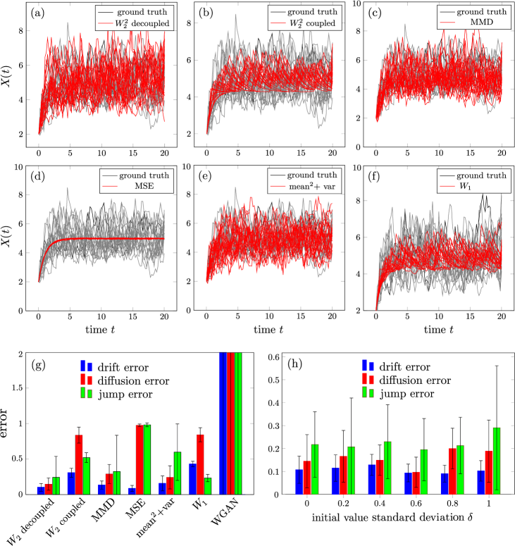
Figure 1: Reconstruction of trajectories and model functions. We define ground truth as $b=4,a=-1,\sigma_{0}=0.4,y_{0}=1$ in Eq. (57), with $T=20.2$ and initial condition $X_{0}=2$. (a-f) ground truth (black) and reconstructed trajectories (red) generated from the learned jump-diffusion process by minimizing different loss functions or using different methods. (g) The reconstruction errors of the drift, diffusion, and jump functions defined in Eqs. (53), (54), and (55). We compare errors from minimizing our temporally decoupled squared $W_{2}$-distance versus those from minimizing the MSE, MMD, mean2+var, the $W_{1}$-distance $W_{1}(\mu,\hat{\mu})$, the squared $W_{2}$-distance $W_{2}^{2}(\mu_{N},\hat{\mu}_{N})$, and the error of results obtained using the WGAN method. The mean and standard deviation of the error for different methods are obtained by repeating the experiment 10 times. (h) The reconstruction errors in the drift, diffusion, and jump functions defined in Eqs. (53), (54), and (55) w.r.t. the standard deviation $\delta$ of the initial condition (Eq. (58)).

We compare our temporally decoupled squared $W_{2}$ distance loss function with the WGAN method and other loss functions (MSE, MMD, mean2+var, $W_{1}$ distance, and the squared $W_{2}$ distance $W_{2}^{2}(\mu_{N},\hat{\mu}_{N})$. The definitions of the other loss functions are given in  F). As shown in Fig. 1(a-f), the trajectories we obtained by minimizing our temporally decoupled squared $W_{2}$-distance accurately match the ground truth trajectories generated by Eq. (57). When using $W_{1}(\mu,\hat{\mu})$, $W_{2}^{2}(\mu,\hat{\mu})$, and MSE loss functions, the reconstructed trajectories deviate qualitatively from those of the ground truth. The solutions of the reconstructed jump-diffusion process generated by the WGAN method are also qualitatively incorrect and are thus not shown here. From Fig. 1(g), minimizing our temporally decoupled squared $W_{2}$-distance gives the smallest reconstruction errors $f-\hat{f},\sigma-\hat{\sigma}$, and $\beta-\hat{\beta}$. The average errors in the reconstructed drift, diffusion, and jump are kept below 0.25. Thus, minimizing our temporally decoupled squared $W_{2}$ distance is found to be more accurate in reconstructing the jump-diffusion process Eq. (57) than other benchmark methods. We also list the average runtime per training iteration as well as the memory usage of different methods in Table 1. The runtime of the WGAN method is significantly longer than that of other methods. Furthermore, the computational cost of using our temporally decoupled squared $W_{2}$ is similar to the cost of using other loss functions while our temporally decoupled squared $W_{2}$ method can accurately reconstruct Eq. (57).

Table 1: The runtime and memory usage of different methods (loss functions) to reconstruct the jump-diffusion process Eq. (57).
Method (loss) temporally
decoupled $W_{2}^{2}$ $W_{2}^{2}$ MMD MSE mean2+var $W_{1}$ WGAN
Average time/iteration (s) 44.5 48.2 59.4 29.8 48.7 39.2 346.3
Average memory use (Gb) 2.61 3.52 2.59 5.00 2.61 2.60 3.34

We test the numerical performance of our temporally decoupled squared $W_{2}$ method when reconstructing Eq. (57) under different initial conditions. Instead of using the same initial condition for all solutions, we sample the initial value from

$$X_{0}\sim\mathcal{N}(2,\delta^{2}),$$ (58)

where $\mathcal{N}(2,\delta^{2})$ is the 1D normal distribution of mean 2 and variance $\delta^{2}$. Using the same hyperparameters in the neural networks and for training (in Table E) as in Example 4.1, we varied the standard deviation $\delta=0,0.2,0.4,0.6,0.8,1$ and implemented the temporally decoupled squared $W_{2}$ distance as a loss function. The results shown in Fig. 1(h) indicate that the reconstruction of Eq. (57) using the squared $W_{2}$ loss function is rather insensitive to “noise”, i.e., the standard deviation $\delta$ in the distribution of the initial condition.

Finally, we also use different values of the parameters $\sigma_{0}$ and $y_{0}$ in the diffusion and drift functions. The reconstructed drift functions $\hat{f}$ remain accurate when $\sigma_{0}$ and $y_{0}$ are varied. When $\sigma_{0},y_{0}$ are small, the corresponding diffusion and jump functions can also be accurately reconstructed; however, when $\sigma_{0},y_{0}$ are large, the reconstruction of the diffusion function can be less accurate because the trajectories for training are more sparsely distributed. Details of the results are given in G.

It was shown in [22] that the accuracy of reconstructing a pure-diffusion process ($\bm{\beta}=0$ in Eq. (1)) can deteriorate if trajectories for training are too sparsely distributed (too few trajectories/too high noise). However, we find that prior information on the drift function in Eq. (1) enables efficient reconstruction even if the number of training trajectories is limited, when the temporally decoupled squared $W_{2}$ method for reconstructing jump-diffusion processes without prior information would otherwise fail. In the next example, we demonstrate enhanced reconstruction performance after incorporating prior information on the drift function of Eq. (1), greatly improving the accuracy of reconstructed diffusion and jump functions.

Example 4.2.

Consider the following 1D jump-diffusion process

$$\text{d}X_{t}=\alpha(X_{t},t)\text{d}t+\sigma(X_{t},t)\text{d}B_{t}+\beta(X_{t},t)\text{d}\tilde{N}_{t},\,\,\,t\in[0,T],$$ (59)

where $\tilde{N}_{t}$ is a 1D compensated Poisson process with intensity $t$. This model, if we set $S_{t}\equiv e^{X_{t}}$, can describe the posited stock returns under a deterministic jump ratio [1]. To test the efficiency of our temporally decoupled squared $W_{2}$-distance method, we set $\alpha\equiv r_{0}=0.05$ (i.e., the drift function to be a constant risk-free interest rate [26]), the initial condition $X_{0}=1$, and $T=5.1$ and explore different forms of the diffusion and jump functions $\sigma(X,t)$ and $\beta(X,t)$. We then input the drift, diffusion, or the jump function $\alpha,\sigma$, or $\beta$ in Eq. (59) as prior information to test how well our method can reconstruct the other terms.

Summarizing, i) we first give no prior information and reconstruct all three functions $\alpha,\sigma$, and $\beta$; ii) we specify the risk-free interest rate $\alpha\equiv r_{0}$ and reconstruct $\sigma$, and $\beta$; iii) we provide the diffusion function $\sigma$ and reconstruct $\alpha$ and $\beta$; iv) we provide the jump function $\beta$ and reconstruct $f$, and $\sigma$. In this example, “const” refers to using a constant diffusion or jump function:

$$\sigma(X,t)\equiv\sigma_{0}\,\,\,\text{or}\,\,\,\beta(X,t)\equiv\beta_{0},$$ (60)

“linear” refers to using a linear diffusion or jump function

$$\sigma(X,t)\equiv\sigma_{0}X\,\,\,\text{or}\,\,\,\beta(X,t)\equiv\beta_{0}X,$$ (61)

and “langevin” refers to using a diffusion or jump function of the following form

$$\sigma(X,t)\equiv\sigma_{0}\sqrt{|X|}\,\,\,\text{or}\,\,\,\beta(X,t)\equiv\beta_{0}\sqrt{|X|}.$$ (62)
Refer to caption
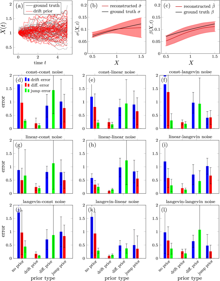
Figure 2: (a) The trajectories generated by the ground truth (black) jump-diffusion process with $\sigma(X,t)\equiv 0.1\sqrt{|X|}\leavevmode\nobreak\ \text{and}\leavevmode\nobreak\ \beta(X,t)\equiv 0.1\sqrt{|X|}$ and given drift function in Eq. (59), plotted against reconstructed trajectories (red) using the same drift function prior. (b-c) The ground truth diffusion and jump functions $\sigma(X,t)\equiv\sigma_{0}\sqrt{|X|}$ and $\beta(X,t)\equiv\beta_{0}\sqrt{|X|}$) shown against the reconstructed functions $\hat{\sigma}(X,t)$ and $\hat{\beta}(X,t)$. (with drift function given as prior). The red curves are the mean $\hat{\sigma}(X,t)$ and $\hat{\beta}(X,t)$ while the shaded bands show their standard deviations, calculated over 5 independent experiments). (d-k) The reconstruction errors of the drift, diffusion, and jump functions without prior information on Eq. (59) or with one of the drift, diffusion, and jump functions given. When the drift function is given, errors in the reconstructed diffusion and jump functions are the smallest in all cases (error bars under “drift prior.”)

To illustrate the reconstruction, we set $\sigma_{0}=\beta_{0}=0.1$ in Eqs. (60),  (61), and (62), and plot in Fig. 2(a) the ground truth solutions (black) generated from Eq. (59) with a given drift function. Using the same drift function, trajectories of the reconstructed jump-diffusion process are shown in red and exhibit a distribution that matches well with that of the ground truth solutions. Moreover, as shown in Fig. 2(b,c), the differences between the learned diffusion and jump functions $\hat{\sigma}(X,t)$ and $\hat{\beta}(X,t)$ and the ground truth diffusion and jump functions $\sigma(X,t)=0.1\sqrt{|X|},\beta(X,t)=0.1\sqrt{|X|}$ are small.

If no prior information on Eq. (59) is given, the average errors for the reconstructed drift, diffusion, and jump functions are 1.412, 0.790, and 0.347, respectively. This high error might arise from training set trajectories that are too noisy or sparsely distributed. However, if the drift function is given, the diffusion and jump functions can be much more accurately reconstructed, leading to relative errors below 0.2 for all three forms of $\sigma(X_{t},t)$ and $\beta(X_{t},t)$ used to define the ground truth [see Fig. 2 (d-k)]. On the other hand, providing the diffusion or jump function does not improve the accuracy of the reconstruction of the other unknown functions in Eq. (59). The average errors of the reconstructed diffusion and jump functions, when different prior information is given, are listed in Table 2.

In  H, we carry out an additional numerical experiment by varying the number of trajectories in the training set. The errors in the reconstructed drift, diffusion, and jump function decrease when the number of trajectories for training increases without any prior information. This indicates that our temporally decoupled squared $W_{2}$ method has the potential to accurately reconstruct Eq. (59) even without prior information provided there are a sufficient number of training trajectories. On the other hand, if the drift function is given as prior information, the errors of the reconstructed diffusion and jump functions are around 0.2 even when only 100 trajectories are used. Therefore, information on the drift function can significantly boost the performance of our temporally decoupled squared $W_{2}$ method, allowing accurate reconstruction of Eq. (59) even when the number of observed trajectories is limited.

In real physical systems, the drift function can often be obtained by measurements over a macroscopic ensemble of trajectories, such as mass-action kinetics if the $X(t)$ in Eq. (1) denotes some physical quantity, e.g., the number density of molecules [27, 28]. Thus, after independently measuring the drift function and inputting it as a prior knowledge, our temporally decoupled squared $W_{2}$-distance method can be used to reconstruct the diffusion and jump functions efficiently.

Table 2: Average errors in the reconstructed drift, diffusion, and jump functions when using the temporally decoupled squared $W_{2}$ distance to reconstruct Eq. (59). The error is taken over 9 possible combinations of different forms of diffusion and jump functions (constant, Langevin, and linear in Eqs. (60), (62), and (61)) in Fig. 2.
Prior info error of reconstructed $\hat{f}$ Error of reconstructed $\hat{\sigma}$ Error of reconstructed $\hat{\beta}$
No prior $1.412(\pm 1.520)$ $0.790(\pm 0.714)$ $0.347(\pm 0.356)$
Given $\alpha(x,t)$ 0 $0.189(\pm 0.124)$ $0.150(\pm 0.080)$
Given $\sigma(x,t)$ $0.771(\pm 0.333)$ 0 $0.939(\pm 0.854)$
Given $\beta(x,t)$ $0.769(\pm 0.520)$ $0.556(\pm 0.393)$ 0

We carry out an extra numerical experiment reconstructing Eq. (59) by varying $\sigma_{0},\beta_{0}$ in Eqs. (60), (61), and (62). With the drift function provided, our temporally decoupled squared $W_{2}$-distance method can accurately reconstruct the diffusion and the jump functions for different values of $\sigma_{0}$ and $\beta_{0}$ in Eqs. (60), (61), and (62). The results are shown in I.

In our last example, we test whether our temporally decoupled squared $W_{2}$-distance can accurately reconstruct a 2D jump-diffusion process with correlated Brownian-type and compensated-Poisson-type noise across the two stochastic variables.

Example 4.3.

We reconstruct the following 2D jump-diffusion process, which is obtained by superimposing a 2D compensated Poisson process $\tilde{\bm{N}}_{t}\coloneqq(\tilde{N}_{1}(t),\tilde{N}_{2}(t))$ onto the pure diffusion process that describes the dynamics of a synthetic data set [4, 29]:

$$\text{d}\bm{X}(t)=-\bm{g}(\bm{X}(t))\text{d}t+\bm{\sigma}(\bm{X}(t))\text{d}\bm{W}_{t}+\bm{\beta}(\bm{X}(t))\text{d}\tilde{\bm{N}}_{t},\,\,\,\bm{X}(t=0)=\bm{X}_{0},\,\,t\in[0,T].$$ (63)

$\tilde{N}_{1}(t)$ and $\tilde{N}_{2}(t)$ are independent and both have intensity $t$. Here, $\bm{X}(t)=(X_{1}(t),X_{2}(t))\in\mathbb{R}^{2}$, $\bm{g}(\bm{X}):\mathbb{R}^{2}\rightarrow\mathbb{R}^{2}$ is the drift function, and $\bm{\sigma},\bm{\beta}:\mathbb{R}^{2}\rightarrow\mathbb{R}^{2\times 2}$ are the diffusion and jump functions, respectively. The drift function $\bm{g}$ is given by

$\displaystyle\bm{g}(\bm{X})=$ $\displaystyle\bigg{(}\frac{1}{\sigma_{1}}\frac{N_{1}}{N_{1}+N_{2}}(X_{1}-\mu_{11})+\frac{1}{\sigma_{2}}\frac{N_{2}}{N_{1}+N_{2}}(X_{1}-\mu_{21}),$ (64)
$\displaystyle\qquad\quad\frac{1}{\sigma_{1}}\frac{N_{1}}{N_{1}+N_{2}}(X_{2}-\mu_{21})+\frac{1}{\sigma_{2}}\frac{N_{2}}{N_{1}+N_{2}}(X_{2}-\mu_{22})\bigg{)}^{T},$
$\displaystyle N_{1}\coloneqq$ $\displaystyle N_{1}(\bm{X})=\frac{1}{\sqrt{2\pi}\sigma_{1}}\exp\Big{(}-\tfrac{(X_{1}-\mu_{11})^{2}}{2\sigma_{1}^{2}}-\tfrac{(X_{2}-\mu_{12})^{2}}{2\sigma_{1}^{2}}\Big{)},$
$\displaystyle N_{2}\coloneqq$ $\displaystyle N_{2}(\bm{X})=\frac{1}{\sqrt{2\pi}\sigma_{2}}\exp\Big{(}-\tfrac{(X_{1}-\mu_{21})^{2}}{2\sigma_{2}^{2}}-\tfrac{(X_{2}-\mu_{22})^{2}}{2\sigma_{2}^{2}}\Big{)}.$

The parameters are set as $\sigma_{1}=1,\sigma_{2}=0.95,\mu_{11}=1.6,\mu_{12}=1.2,\mu_{21}=1.8,\mu_{22}=1.0$. We set $T=10.2$ and an initial condition $\bm{X}_{0}=(1.7,1.1)$. We take the correlated diffusivity as

$$\bm{\sigma}=\begin{bmatrix}\sigma_{0}\sqrt{|X_{1}|}&c_{1}\sigma_{0}\sqrt{|X_{2}|}\\ c_{1}\sigma_{0}\sqrt{|X_{1}|}&\sigma_{0}\sqrt{|X_{2}|}\end{bmatrix},$$ (65)

and the jump function of the compensated Poisson process as

$$\bm{\beta}=\begin{bmatrix}\beta_{0}&c_{2}\beta_{0}\\ c_{2}\beta_{0}&\beta_{0}\\ \end{bmatrix}.$$ (66)

Here, $c_{1}$ and $c_{2}$ determine the correlations of Brownian noise and compensated Poisson process across the two dimensions, respectively. Specifically, when $c_{1}=0$ (or $c_{2}=0$), the Brownian (or compensated Poisson) noise in each variable is independent of the other; when $c_{1}=1$ (or $c_{2}=1$), the Brownian-type (or compensated-Poisson-type) noise across the two dimensions are linearly dependent; when $c_{1}=-1$ (or $c_{2}=-1$), the Brownian-type (or compensated-Poisson-type) noise across the two dimensions are perfectly negatively correlated.

From Example 4.2, imposing a prior on the drift function can greatly improve the accuracy of the reconstructed diffusion and jump functions. Thus, we input $\bm{g}(\bm{X})$ defined in Eq. (64) as prior information. Since the jump-diffusion process described by Eq. (63) is two-dimensional, we use the following error metric to measure the errors in the diffusion and jump functions:

$$\text{diffusion error}=\frac{\sum_{i=0}^{N}\sum_{j=1}^{M_{s}}\|\bm{\sigma}\bm{\sigma}^{T}(x_{j}(t_{i}),t_{i})-\hat{\bm{\sigma}}\hat{\bm{\sigma}}^{T}(x_{j}(t_{i}),t_{i})\|^{2}_{F}}{\sum_{i=0}^{N}\sum_{j=1}^{M_{s}}\|\hat{\bm{\sigma}}\hat{\bm{\sigma}}^{T}(x_{j}(t_{i}),t_{i})\|_{F}^{2}};$$ (67)
$$\text{jump error}=\frac{\sum_{i=0}^{N}\sum_{j=1}^{M_{s}}\|\bm{\beta}\bm{\beta}^{T}(x_{j}(t_{i}),t_{i})-\hat{\bm{\beta}}\hat{\bm{\beta}}^{T}(x_{j}(t_{i}),t_{i})\|^{2}_{F}}{\sum_{i=0}^{N}\sum_{j=1}^{M_{s}}\|\hat{\bm{\beta}}\hat{\bm{\beta}}^{T}(x_{j}(t_{i}),t_{i})\|_{F}^{2}}.$$ (68)

Here, $\|\cdot\|_{F}$ denotes the Frobenius norm of a matrix. We set $\sigma_{0}=0.1,\beta_{0}=0.1$ in Eqs. (65) and (66). Different values of $c_{1},c_{2}$ are used to tune the correlations to explore how they affect the reconstruction of the jump-diffusion process.

Refer to caption
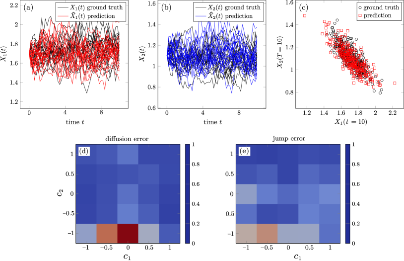
Figure 3: (a-b) Solutions generated by the reconstructed jump-diffusion process using our temporally decoupled squared $W_{2}$ method versus solutions generated by the ground truth Eq. (63). (c) The reconstructed $\hat{\bm{X}}(t=10)$ versus the ground truth $\bm{X}(t=10)$. In (a-c), $c_{1}=c_{2}=-0.5$. (d) The error (Eq. (67)) between the ground truth diffusion function $\bm{\sigma}$ and the reconstructed diffusion function $\hat{\bm{\sigma}}$. (e) The error (Eq. (68)) between the ground truth jump function $\bm{\beta}$ and the reconstructed diffusion function $\hat{\bm{\beta}}$. In (d-e), the errors are averaged over 5 independent experiments.

Figs. 3(a-c) show that solutions generated by our reconstructed jump-diffusion process with the temporally decoupled squared $W_{2}$ loss function match well with solutions generated by the 2D jump-diffusion process Eq. (63) ($c_{1}=c_{2}=-0.5$ in Eqs. (65) and (66)). Figs. (3)(d-e) indicate that when the drift function $\bm{g}(\bm{X}(t))$ is given, our temporally decoupled squared $W_{2}$ method can accurately reconstruct the diffusion and jump functions for most combinations of $c_{1},c_{2}$ The average errors in the diffusion and jump functions averaged over all combinations of $c_{1},c_{2}$ are 0.197 and 0.210, respectively. Also, the final distribution of the reconstructed $\hat{\bm{X}}(t)$ aligns well with the ground truth $\bm{X}(t)$.

In  J, we implement our reconstruction method by using different numbers of hidden layers and different numbers of neurons in each layer for the neural-network-parameterized approximation to the diffusion and jump functions $\bm{\sigma}$ and $\bm{\beta}$. We find that with the drift function given as prior information, increasing the number of neurons per layer can improve the accuracy of the reconstructed diffusion and the jump function of the 2D jump-diffusion process Eq. (63). Increasing the number of hidden layers also leads to a more accurate reconstruction of the diffusion and jump function when the number of hidden layers is smaller than three; however, after three hidden layers, increasing their number leads to less accuracy of the reconstructed $\bm{\sigma}$ and $\bm{\beta}$. Setting the number of hidden layers to three and the number of neurons per layer to about 400 leads to excellent reconstruction of $\bm{\sigma}$ and $\bm{\beta}$. However, larger numbers of hidden layers or neurons per hidden layer demand more memory usage and lead to longer runtimes. The optimal network architecture for reconstructing the diffusion and jump functions is worth further investigation.

5 Summary & conclusions

In this paper, we proposed and analyzed Wasserstein-distance-based loss functions for reconstructing jump-diffusion processes. Specifically, we showed that a temporally decoupled squared $W_{2}$-distance $\tilde{W}_{2}^{2}(\mu,\hat{\mu})$ defined in Eq. (22) provides both upper and lower bounds for errors in the drift, diffusion, and jump functions $\bm{f}-\hat{\bm{f}}$, $\bm{\sigma}-\hat{\bm{\sigma}}$, and $\bm{\beta}-\hat{\bm{\beta}}$ when approximating a jump-diffusion process Eq. (1) by another jump-diffusion process 5. Moreover, the temporally decoupled squared $W_{2}$-distance can be efficiently evaluated using finite-sample finite-time-point observations, which yields an easy-to-calculate loss function for reconstructing jump-diffusion processes.

Through several numerical experiments, we showed that minimizing our proposed temporally decoupled squared $W_{2}$-distance loss performs much better than other commonly used loss functions and methods for jump-diffusion process reconstruction using parameterized neural networks. Furthermore, we showed that if we imposed prior knowledge on the drift function of the jump-diffusion process, then the diffusion and jump functions could be more accurately reconstructed.

Although we analyzed a 2D stochastic jump-diffusion process, investigating how our temporally decoupled squared $W_{2}$ method performs in higher dimensional jump-diffusion processes with more general noise correlation matrices should be further explored. Such analyses would inform how our approach can be directly applied to real-world multi-dimensional jump-diffusion models with applications in finance, biology, physics, and other disciplines. Similarly, how the Wasserstein distance can be adapted to reconstruct other stochastic processes such as Lévy walks involving compound Poisson process [30, 31] is a potentially fruitful area of further investigation. Reconstructing such processes could require inferring the intensity of the Poisson process, which is nontrivial and would require consideration of differentiation w.r.t. “discrete randomness” [32].

Data availability statement

No data was used during this study. All code will be published upon acceptance of this manuscript.

Conflict of interest

The authors declare that they have no conflicts of interest to report regarding the present study.

References

References

  • [1] Robert C Merton. Option pricing when underlying stock returns are discontinuous. Journal of Financial Economics, 3(1-2):125–144, 1976.
  • [2] Jiwook Jang. Jump diffusion processes and their applications in insurance and finance. Insurance: Mathematics and Economics, 41(1):62–70, 2007.
  • [3] Koichi Maekawa, Sangyeol Lee, Takayuki Morimoto, and Ken-ichi Kawai. Jump diffusion model with application to the Japanese stock market. Mathematics and Computers in Simulation, 78(2-3):223–236, 2008.
  • [4] Jia-Xing Gao, Zhen-Yi Wang, Michael Q Zhang, Min-Ping Qian, and Da-Quan Jiang. A data-driven method to learn a jump diffusion process from aggregate biological gene expression data. Journal of Theoretical Biology, 532:110923, 2022.
  • [5] Almaz Tesfay, Tareq Saeed, Anwar Zeb, Daniel Tesfay, Anas Khalaf, and James Brannan. Dynamics of a stochastic COVID-19 epidemic model with jump-diffusion. Advances in Difference Equations, 2021(1):1–19, 2021.
  • [6] Sima Mehri and Michael Scheutzow. A stochastic Gronwall lemma and well-posedness of path-dependent SDEs driven by martingale noise. arXiv preprint arXiv:1908.10646, 2019.
  • [7] Bruno Casella and Gareth O Roberts. Exact simulation of jump-diffusion processes with Monte Carlo applications. Methodology and Computing in Applied Probability, 13:449–473, 2011.
  • [8] Steve AK Metwally and Amir F Atiya. Using Brownian bridge for fast simulation of jump-diffusion processes and barrier options. The Journal of Derivatives, 10(1):43–54, 2002.
  • [9] Steven G Kou and Hui Wang. First passage times of a jump diffusion process. Advances in Applied Probability, 35(2):504–531, 2003.
  • [10] Di Zhang and Roderick VN Melnik. First passage time for multivariate jump-diffusion processes in finance and other areas of applications. Applied Stochastic Models in Business and Industry, 25(5):565–582, 2009.
  • [11] Leonardo Rydin Gorjão, Jan Heysel, Klaus Lehnertz, and M Reza Rahimi Tabar. Analysis and data-driven reconstruction of bivariate jump-diffusion processes. Physical Review E, 100(6):062127, 2019.
  • [12] Cyrus A Ramezani and Yong Zeng. Maximum likelihood estimation of asymmetric jump-diffusion processes: application to security prices. Available at SSRN 606361, 1998.
  • [13] Leonardo Rydin Gorjão, Dirk Witthaut, and Pedro G Lind. jumpdiff: A Python library for statistical inference of jump-diffusion processes in observational or experimental data sets. Journal of Statistical Software, 105:1–22, 2023.
  • [14] Xuechen Li, Ting-Kam Leonard Wong, Ricky TQ Chen, and David Duvenaud. Scalable gradients for stochastic differential equations. In International Conference on Artificial Intelligence and Statistics, pages 3870–3882. PMLR, 2020.
  • [15] Belinda Tzen and Maxim Raginsky. Neural stochastic differential equations: deep latent Gaussian models in the diffusion limit. arXiv preprint arXiv:1905.09883, 2019.
  • [16] Anh Tong, Thanh Nguyen-Tang, Toan Tran, and Jaesik Choi. Learning fractional white noises in neural stochastic differential equations. In Advances in Neural Information Processing Systems, volume 35, pages 37660–37675, 2022.
  • [17] Patrick Kidger, James Foster, Xuechen Li, and Terry J Lyons. Neural SDEs as infinite-dimensional GANs. In International Conference on Machine Learning, pages 5453–5463. PMLR, 2021.
  • [18] Yuan Chen and Dongbin Xiu. Learning stochastic dynamical system via flow map operator. arXiv preprint arXiv:2305.03874, 2023.
  • [19] Jean-Christophe Breton and Nicolas Privault. Wasserstein distance estimates for jump-diffusion processes. Stochastic Processes and their Applications, page 104334, 2024.
  • [20] Cédric Villani et al. Optimal transport: old and new, volume 338. Springer, 2009.
  • [21] Wenbo Zheng, Fei-Yue Wang, and Chao Gou. Nonparametric different-feature selection using Wasserstein distance. In 2020 IEEE 32nd International Conference on Tools with Artificial Intelligence (ICTAI), pages 982–988. IEEE, 2020.
  • [22] Mingtao Xia, Xiangting Li, Qijing Shen, and Tom Chou. Squared Wasserstein-2 distance for efficient reconstruction of stochastic differential equations. arXiv preprint arXiv:2401.11354, 2024.
  • [23] Benjamin Arras and Christian Houdré. On Stein’s method for infinitely divisible laws with finite first moment. Springer, 2019.
  • [24] Nicolas Fournier and Arnaud Guillin. On the rate of convergence in Wasserstein distance of the empirical measure. Probability Theory and Related Fields, 162(3-4):707–738, 2015.
  • [25] DC Dowson and BV Landau. The Fréchet distance between multivariate normal distributions. Journal of Multivariate Analysis, 12(3):450–455, 1982.
  • [26] John Hull. Options, futures, and other derivative securities, volume 7. Prentice Hall Englewood Cliffs, NJ, 1993.
  • [27] Andrei B Koudriavtsev, Reginald F Jameson, and Wolfgang Linert. The law of mass action. Springer Science & Business Media, 2011.
  • [28] Vijaysekhar Chellaboina, Sanjay P Bhat, Wassim M Haddad, and Dennis S Bernstein. Modeling and analysis of mass-action kinetics. IEEE Control Systems Magazine, 29(4):60–78, 2009.
  • [29] Shaojun Ma, Shu Liu, Hongyuan Zha, and Haomin Zhou. Learning stochastic behaviour from aggregate data. In International Conference on Machine Learning, pages 7258–7267. PMLR, 2021.
  • [30] Jean Bertoin. Lévy processes, volume 121. Cambridge university press Cambridge, 1996.
  • [31] Ole E Barndorff-Nielsen, Thomas Mikosch, and Sidney I Resnick. Lévy processes: theory and applications. Springer Science & Business Media, 2001.
  • [32] Gaurav Arya, Moritz Schauer, Frank Schäfer, and Christopher Rackauckas. Automatic differentiation of programs with discrete randomness. Advances in Neural Information Processing Systems, 35:10435–10447, 2022.
  • [33] Philippe Clement and Wolfgang Desch. An elementary proof of the triangle inequality for the Wasserstein metric. Proceedings of the American Mathematical Society, 136(1):333–339, 2008.
  • [34] Rémi Flamary, Nicolas Courty, Alexandre Gramfort, Mokhtar Z. Alaya, Aurélie Boisbunon, Stanislas Chambon, Laetitia Chapel, Adrien Corenflos, Kilian Fatras, Nemo Fournier, Léo Gautheron, Nathalie T.H. Gayraud, Hicham Janati, Alain Rakotomamonjy, Ievgen Redko, Antoine Rolet, Antony Schutz, Vivien Seguy, Danica J. Sutherland, Romain Tavenard, Alexander Tong, and Titouan Vayer. POT: Python optimal transport. Journal of Machine Learning Research, 22(78):1–8, 2021.
  • [35] Yujia Li, Kevin Swersky, and Rich Zemel. Generative moment matching networks. In International Conference on Machine Learning, pages 1718–1727. PMLR, 2015.
  • [36] Xavier Glorot and Yoshua Bengio. Understanding the difficulty of training deep feedforward neural networks. In Proceedings of the thirteenth international conference on artificial intelligence and statistics, pages 249–256. JMLR Workshop and Conference Proceedings, 2010.
  • [37] Kaiming He, Xiangyu Zhang, Shaoqing Ren, and Jian Sun. Deep residual learning for image recognition. In Proceedings of the IEEE conference on computer vision and pattern recognition, pages 770–778, 2016.

Appendix A Proof to Theorem 2.1

Here, we provide proof for Theorem 2.1. Our strategy is similar to that used in the proof of the stochastic Gronwall lemma (Theorem 2.2 in [6]). First, we apply the Ito’s lemma to

$\displaystyle\big{|}X_{i}(t)-\tilde{X}_{i}(t)\big{|}^{2}=$ $\displaystyle 2\int_{0}^{t}\big{(}X_{i}(s^{-})-\tilde{X}_{i}(s^{-})\big{)}\big{(}f_{i}(\bm{X}(s^{-}),s^{-})-\hat{f}_{i}(\tilde{\bm{X}}(s^{-}),s^{-})\big{)}\text{d}s$ (69)
$\displaystyle+2\int_{0}^{t}\sum_{j=1}^{m}\big{(}X_{i}(s^{-})-\tilde{X}_{i}(s^{-})\big{)}\big{(}\sigma_{i,j}(\bm{X}(s^{-}),s^{-})-\hat{\sigma}_{i,j}(\tilde{\bm{X}}_{i}(s^{-}),s^{-})\big{)}\text{d}B_{j,s}$
$\displaystyle+2\int_{0}^{t}\int_{U}\big{(}X_{i}(s^{-})-\tilde{X}_{i}(s^{-})\big{)}\big{(}\beta_{i}(\bm{X}(s^{-}),\xi,s^{-})-\hat{\beta}_{i}(\hat{\bm{X}}(s^{-}),\xi,s^{-})\big{)}\text{d}\tilde{N}\big{(}\text{d}s,\nu(\text{d}\xi)\big{)}$
$\displaystyle+\int_{0}^{t}\sum_{j=1}^{m}\big{(}\sigma_{i,j}(X_{i}(s^{-}),s^{-})-\hat{\sigma}_{i,j}(\tilde{X}_{i}(s^{-}),s^{-})\big{)}^{2}\text{d}s$
$\displaystyle+\int_{0}^{t}\int_{U}\big{(}\beta_{i}(X_{i}(s^{-}),\xi,s^{-})-\hat{\beta}_{i,j}(\tilde{X}_{i}(s^{-}),\xi,s^{-})\big{)}^{2}\nu(\text{d}\xi)\text{d}s.$

Note that

$\displaystyle f_{i}(\bm{X}(s^{-}),s^{-})-\hat{f}_{i}(\tilde{\bm{X}}(s^{-}),s^{-})=$ $\displaystyle\big{(}f_{i}(\bm{X}(s^{-}),s^{-})-\hat{f}_{i}(\bm{X}(s^{-}),s^{-})\big{)}$ (70)
$\displaystyle\qquad\quad+\big{(}\hat{f}_{i}(\bm{X}(s^{-}),s^{-})-\hat{f}_{i}(\tilde{\bm{X}}(s^{-}),s^{-})\big{)},$
$\displaystyle\sigma_{i,j}(\bm{X}(s^{-}),s^{-})-\hat{\sigma}_{i,j}(\tilde{\bm{X}}(s^{-}),s^{-})=$ $\displaystyle\big{(}\sigma_{i,j}(\bm{X}(s^{-}),s^{-})-\hat{\sigma}_{i,j}(\bm{X}(s^{-}),s^{-})\big{)}$
$\displaystyle\qquad\quad+\big{(}\hat{\sigma}_{i,j}(\bm{X}(s^{-}),s^{-})-\hat{\sigma}_{i,j}(\tilde{\bm{X}}(s^{-}),s^{-})\big{)},$
$\displaystyle\beta_{i}(\bm{X}(s^{-}),\xi,s^{-})-\hat{\beta}_{i}(\tilde{\bm{X}}(s^{-}),\xi,s^{-})=$ $\displaystyle\big{(}\beta_{i}(\bm{X}(s^{-}),\xi,s^{-})-\hat{\beta}_{i}(\bm{X}(s^{-}),\xi,s^{-})\big{)}$
$\displaystyle\qquad\quad+\big{(}\hat{\beta}_{i}(\bm{X}(s^{-}),\xi,s^{-})-\hat{\beta}_{i}(\tilde{\bm{X}}(s^{-}),\xi,s^{-})\big{)}.$

Using the Lipschitz conditions on the drift, diffusion, and jump functions $\hat{\bm{f}},\hat{\bm{\sigma}}$, and $\hat{\bm{\beta}}$ in Assumption 2.1 as well as the Cauchy inequality, from Eq. (69) and 70, we find

$\displaystyle\big{|}\bm{X}(t)-\tilde{\bm{X}}(t)\big{|}_{2}^{2}$ $\displaystyle=\sum_{i=1}^{d}\big{(}X_{i}(t)-\hat{X}_{i}(t)\big{)}^{2}$ (71)
$\displaystyle\leq\big{(}2\overline{f}+2\overline{\sigma}m+2\nu(U)\overline{\beta}+1+m+\nu(U)\big{)}\sum_{i=1}^{d}\int_{0}^{t}\big{(}X_{i}(s^{-})-\tilde{X}_{i}(s^{-})\big{)}^{2}\text{d}s$
$\displaystyle\quad+\sum_{i=1}^{d}\int_{0}^{t}\big{|}f_{i}(\bm{X}(s^{-}),s^{-})-\hat{f}_{i}\bm{X}(s^{-}),s^{-})\big{|}^{2}\text{d}s$
$\displaystyle\quad+2\sum_{i=1}^{d}\int_{0}^{t}\sum_{j=1}^{m}\big{|}\sigma_{i,j}(\bm{X}(s^{-}),s^{-})-\hat{\sigma}_{i,j}(\bm{X}(s^{-}),s^{-})\big{|}^{2}\text{d}s$
$\displaystyle\quad+2\sum_{i=1}^{d}\int_{0}^{t}\int_{U}\big{|}\beta_{i}(\bm{X}(s^{-}),\xi,s^{-})-\hat{\beta}_{i}(\bm{X}(s^{-}),\xi,s^{-})\big{|}^{2}\nu(\text{d}\xi)\text{d}s$
$\displaystyle\quad+2\sum_{i=1}^{d}\int_{0}^{t}\sum_{j=1}^{m}\big{(}X_{i}(s^{-})-\tilde{X}_{i}(s^{-})\big{)}\big{(}\sigma_{i,j}(\bm{X}(s^{-}),s^{-})-\hat{\sigma}_{i,j}(\tilde{\bm{X}}_{i}(s^{-}),s^{-})\big{)}\text{d}B_{j,s}$
$\displaystyle\quad+2\sum_{i=1}^{d}\!\int_{0}^{t}\!\int_{U}\big{(}X_{i}(s^{-})-\tilde{X}_{i}(s^{-})\big{)}\big{(}\beta_{i}(\bm{X}(s^{-}),\xi,s^{-})-\hat{\beta}_{i}(\tilde{\bm{X}}(s^{-}),\xi,s^{-})\big{)}\text{d}\tilde{N}\big{(}\text{d}s,\nu(\text{d}\xi)\big{)}.$

From Assumption 2.1 and the conditions in Theorem 2.1, the second, third, and fourth terms on the RHS of Eq. (71) are adapted and non-decreasing w.r.t. $t$; the fifth and sixth terms on the RHS of Eq. (71) are martingales. Thus, by taking the expectation of both sides of Eq. (71), we find

$$\mathbb{E}\Big{[}\big{|}\bm{X}(t)-\tilde{\bm{X}}(t)\big{|}_{2}^{2}\Big{]}\leq\big{(}2\overline{f}+1+(2\overline{\sigma}+1)m+(2\overline{\beta}+1)\nu(U)\big{)}\int_{0}^{t}\mathbb{E}\Big{[}\big{|}\bm{X}(s)-\tilde{\bm{X}}(s)\big{|}_{2}^{2}\Big{]}\text{d}s+\mathbb{E}[H(t)],$$ (72)

where $H(t)$ is defined in Eq. (14). Applying Gronwall’s lemma to $u(t)\coloneqq\mathbb{E}\Big{[}\big{|}\bm{X}(t)-\tilde{\bm{X}}(t)\big{|}_{2}^{2}\Big{]}$ and noticing that $\mathbb{E}[H(t)]$ is non-decreasing w.r.t. $t$, we conclude that

$$u(t)\leq\mathbb{E}\Big{[}\big{|}\bm{X}(t)-\tilde{\bm{X}}(t)\big{|}^{2}\,\Big{|}\,\bm{X}(0)\Big{]}\leq\exp\Big{(}(2\overline{f}+1+(2\overline{\sigma}+1)m+(2\overline{\beta}+1)\nu(E))T\Big{)}\cdot\mathbb{E}\big{[}H(T)\,|\,\bm{X}(0)\big{]},$$ (73)

which proves Eq. (13).

Appendix B Proof to Theorem 2.2

Here, we shall provide proof of Theorem 2.2, which generalizes Theorem 2 in [22] for pure diffusion processes. Denote

$$\Omega_{N}\coloneqq\{\bm{Y}(t)|\bm{Y}(t)=\bm{Y}(t_{i})\,\,\,t\in[t_{i},t_{i+1}),i<N-1;\,\,\bm{Y}(t)=\bm{Y}(t_{i}),\,\,\,t\in[t_{i},t_{i+1}]\}$$ (74)

to be the space of piecewise functions. Clearly, it is a subspace of $L^{2}([0,T];\mathbb{R}^{d})$. Also, the embedding map from $\Omega_{N}$ to $L^{2}([0,T];\mathbb{R}^{d})$ preserves the $\|\cdot\|$ norm, which enables us to define the measures on $\mathcal{B}(L^{2}([0,T];\mathbb{R}^{d}))$ induced by the measures $\mu_{N},\hat{\mu}_{N}$. For simplicity, we shall still denote those induced measures by $\mu_{N},\hat{\mu}_{N}$.

Suppose $\bm{X}(t),\hat{\bm{X}}(t)$ are generated by two jump-diffusion processes defined by Eq. (1) and Eq. (5). The inequality Eq. (19) is a direct result of the triangular inequality for the Wasserstein distance [33] because $\bm{X},\bm{X}_{N},\hat{\bm{X}},\hat{\bm{X}}_{N}\in L^{2}([0,T];\mathbb{R}^{d})$.

Next, we prove Eq. (21). Because $\bm{X}_{N}(t)=I_{N}\bm{X}(t)$ (defined in Eq. (18)), we choose a specific coupling measure, i.e. the coupled distribution, $\pi$ of $\mu,\mu_{N}$ that is essentially the “original” probability distribution. To be more specific, for an abstract probability space $(\Omega,\mathcal{A},p)$ associated with ${\bm{X}}$, $\mu$ and $\mu_{N}$ can be characterized by the pushforward of $p$ via ${\bm{X}}$ and ${\bm{X}}_{N}$ respectively, i.e., $\mu={\bm{X}}_{*}p$, defined by $\forall A\in\mathcal{B}\big{(}\tilde{\Omega}_{N}\big{)}$, elements in the Borel $\sigma$-algebra of $\tilde{\Omega}_{N}$,

$$\mu(A)={\bm{X}}_{*}p(A)\coloneqq p\big{(}{\bm{X}}^{-1}(A)\big{)},$$ (75)

where $\bm{X}$ is interpreted as a measurable map from $\Omega$ to $\tilde{\Omega}_{N}$, and $\bm{X}^{-1}(A)$ is the preimage of $A$ under $\bm{X}$. Then, the coupling $\pi$ is defined by

$$\pi=({\bm{X}},{\bm{X}}_{N})_{*}p,$$ (76)

where $({\bm{X}},{\bm{X}}_{N})$ are interpreted as a measurable map from $\Omega$ to $\tilde{\Omega}_{N}\times\tilde{\Omega}_{N}$. One can readily verify that the marginal distributions of $\pi$ are $\mu$ and $\mu_{N}$ respectively. Therefore, the squared $W_{2}^{2}(\mu,\mu_{N})$ can be bounded by

$$W_{2}^{2}(\mu,\mu_{N})\leq\sum_{i=1}^{N}\int_{t_{i-1}}^{t_{i}}\!\mathbb{E}\Big{[}\big{|}\bm{X}(t)-\bm{X}_{N}(t)\big{|}_{2}^{2}\Big{]}\text{d}t=\sum_{i=1}^{N}\int_{t_{i-1}}^{t_{i}}\sum_{\ell=1}^{d}\mathbb{E}\Big{[}\big{(}X_{\ell}(t)-X_{N,\ell}(t)\big{)}^{2}\Big{]}\text{d}t$$ (77)

For each $\ell=1,...,d$, by using the Itô’s isometry and the orthogonality condition of the compensated Poisson process $\tilde{N}$ (in Assumption 2.1), we have

$\displaystyle\sum_{i=1}^{N}\int_{t_{i-1}}^{t_{i}}\!\mathbb{E}\big{[}\big{(}X_{\ell}(t)-X_{N,\ell}(t)\big{)}^{2}\big{]}\text{d}t\leq$ $\displaystyle\sum_{i=1}^{N}\int_{t_{i-1}}^{t_{i}}\mathbb{E}\bigg{[}\Big{(}\medint\int_{t_{i}}^{t}f_{\ell}(\bm{X}(r^{-}),r^{-})\text{d}r\Big{)}^{2}\bigg{]}\text{d}t$ (78)
$\displaystyle+\sum_{i=1}^{N}\int_{t_{i-1}}^{t_{i}}\mathbb{E}\bigg{[}\Big{(}\medint\int_{t_{i}}^{t}\sum_{j=1}^{m}\sigma_{\ell,j}(\hat{X}(r^{-}),r^{-})\text{d}B_{j,r}\Big{)}^{2}\bigg{]}\text{d}t$
$\displaystyle+\sum_{i=1}^{N}\int_{t_{i-1}}^{t_{i}}\mathbb{E}\bigg{[}\Big{(}\medint\int_{t_{i}}^{t}\medint\int_{U}\beta_{\ell}(\bm{X}(r^{-}),\xi,r^{-})\tilde{N}(\text{d}r,\nu(\text{d}\xi))\Big{)}^{2}\bigg{]}\text{d}t$
$\displaystyle\leq$ $\displaystyle\sum_{i=1}^{N}\big{(}\Delta t_{i-1}\big{)}^{2}\mathbb{E}\Big{[}\medint\int_{t_{i-1}}^{t_{i}}\!f_{\ell}^{2}\text{d}t\Big{]}+\sum_{i=1}^{N}\big{(}\Delta t_{i-1}\big{)}^{2}\sum_{j=1}^{m}\mathbb{E}\Big{[}\medint\int_{t_{i-1}}^{t_{i}}\!\sigma_{\ell,j}^{2}\text{d}t\Big{]}$
$\displaystyle+\sum_{i=1}^{N}\Delta t_{i-1}\mathbb{E}\Big{[}\medint\int_{t_{i-1}}^{t_{i}}\medint\int_{U}\beta_{\ell}^{2}\nu(\text{d}\xi)\text{d}t\Big{]},$

where $\Delta t_{i-1}\coloneqq t_{i}-t_{i-1}$. Summing over $\ell$, we have

$$\sqrt{\sum_{i=1}^{N}\medint\int_{t_{i-1}}^{t_{i}}\mathbb{E}\Big{[}\big{|}\bm{X}(t)-\bm{X}_{N}(t)\big{|}_{2}^{2}\Big{]}\text{d}t}\leq\sqrt{F\Delta t^{2}+\Sigma\Delta t+B\Delta t},$$ (79)

where $\Delta t\coloneqq\max_{0\leq i\leq N-1}(t_{i+1}-t_{i})$. Similarly, we can show that

$$W_{2}(\hat{\mu},\hat{\mu}_{N})\leq\sqrt{\hat{F}\Delta t^{2}+{\hat{\Sigma}}\Delta t+{\hat{B}}\Delta t}.$$ (80)

Plugging Eq. (79) and Eq. (80) into Eq. (19), we have proved Eq. (21).

Appendix C Proof to Theorem 3.1

Here, we provide proof to Theorem 3.1. The proof builds upon and generalizes the proof of Theorem 3 in [22] for pure diffusion processes to jump-diffusion processes. First, notice that

$$\mathbb{E}\Big{[}\big{|}\bm{X}(t)-\hat{\bm{X}}(t)\big{|}_{2}^{2}\Big{]}\leq 2(FT+\hat{F}T+\Sigma+\hat{\Sigma}+B+\hat{B})<\infty,\,\,\,\forall t\in[0,T]$$ (81)

where $F,\hat{F},\Sigma,\hat{\Sigma},B,\hat{B}$ are defined in Eq. (20). By applying Theorem 2.2, for any $t_{i},i=1,2,...,N$, denoting $\Delta t_{i}\coloneqq t_{i}-t_{i-1}$ , we have

$\displaystyle\inf_{\pi_{i}}\sqrt{\mathbb{E}_{\pi_{i}}\big{[}|\bm{X}(t_{i})-\hat{\bm{X}}(t_{i})|_{2}^{2}\big{]}\Delta t_{i}}$ $\displaystyle-\sqrt{F_{i}(\Delta t_{i})^{2}+\Sigma_{i}\Delta t_{i}+B_{i}\Delta t_{i}}-\sqrt{\hat{F}_{i}(\Delta t_{i})^{2}+\hat{\Sigma}_{i}\Delta t_{i}+\hat{B}_{i}\Delta t_{i}}$ (82)
$\displaystyle\leq W_{2}\big{(}\bm{\mu}_{i},\hat{\bm{\mu}}_{i}\big{)}$
$\displaystyle\leq\inf_{\pi_{i}}\sqrt{\mathbb{E}_{\pi_{i}}\big{[}|\bm{X}(t_{i})-\hat{\bm{X}}(t_{i})|_{2}^{2}\big{]}\Delta t_{i}}+\!\sqrt{F_{i}(\Delta t_{i})^{2}+\Sigma_{i}\Delta t_{i}+B_{i}\Delta t_{i}}$
$\displaystyle\hskip 119.50148pt+\!\sqrt{\hat{F}_{i}(\Delta t_{i})^{2}+\hat{\Sigma}_{i}\Delta t_{i}+\hat{B}_{i}\Delta t_{i}},$

where $\bm{\mu}_{i},\hat{\bm{\mu}}_{i}$ are the distributions for $\bm{X}(t),t\in[t_{i},t_{i+1})$ and $\hat{\bm{X}}(t),t\in[t_{i},t_{i+1})$, respectively. Additionally, from Eq. (30), we have

$\displaystyle\sum_{i=0}^{N-1}F_{i}=$ $\displaystyle F<\infty,\,\,\,\sum_{i=0}^{N-1}\Sigma_{i}=\Sigma<\infty,\,\,\sum_{i=0}^{N-1}B_{i}=B<\infty$ (83)
$\displaystyle\sum_{i=0}^{N-1}\hat{F}_{i}=$ $\displaystyle\hat{F}<\infty,\,\,\,\sum_{i=0}^{N-1}\hat{\Sigma}_{i}=\hat{\Sigma}<\infty,\,\,\,\sum_{i=0}^{N-1}\hat{B}_{i}=\hat{B}<\infty.$

From the inequality 82, we have

$\displaystyle W_{2}^{2}(\bm{\mu}_{i},\hat{\bm{\mu}}_{i})\leq$ $\displaystyle\inf_{\pi_{i}}\mathbb{E}_{\pi_{i}}\big{[}|\bm{X}(t_{i})-\hat{\bm{X}}(t_{i})|_{2}^{2}\big{]}\Delta t_{i}$ (84)
$\displaystyle\,\,+2\inf_{\pi_{i}}\sqrt{\mathbb{E}_{\pi_{i}}\big{[}|\bm{X}(t_{i})-\hat{\bm{X}}(t_{i})|_{2}^{2}\big{]}}\,\Delta t_{i}\Big{[}\sqrt{F_{i}\Delta t_{i}+\Sigma_{i}+B_{i}}+\!\sqrt{\hat{F}\Delta t_{i}+\hat{\Sigma}_{i}+\hat{B}_{i}}\Big{]}$
$\displaystyle\qquad+2\Delta t_{i}\Big{(}F_{i}\Delta t_{i}+\Sigma_{i}+B_{i}+\hat{F}_{i}\Delta t_{i}+\hat{\Sigma}_{i}+\hat{B}_{i}\Big{)}$
$\displaystyle W_{2}^{2}(\bm{\mu}_{i},\hat{\bm{\mu}}_{i})\geq$ $\displaystyle\inf_{\pi_{i}}\mathbb{E}_{\pi_{i}}\big{[}|\bm{X}(t_{i})-\hat{\bm{X}}(t_{i})|_{2}^{2}\big{]}\Delta t_{i}$
$\displaystyle\quad-2W_{2}(\bm{\mu}_{i},\hat{\bm{\mu}}_{i})\Delta t_{i}\Big{[}\sqrt{F_{i}\Delta t_{i}+\Sigma_{i}+B_{i}}+\!\sqrt{\hat{F}\Delta t_{i}+\hat{\Sigma}_{i}+\hat{B}_{i}}\Big{]}$
$\displaystyle\qquad\,-2\Delta t_{i}\Big{(}F_{i}\Delta t_{i}+\Sigma_{i}+B_{i}+\hat{F}_{i}\Delta t_{i}+\hat{\Sigma}_{i}+\hat{B}_{i}\Big{)}$

Specifically, from the assumption given in Eq. (81) and Eq. (82), we conclude that

$$W_{2}(\bm{\mu}_{i},\hat{\bm{\mu}}_{i})\leq\sqrt{\Delta t_{i}}\Big{(}M+\sqrt{F\Delta t_{i}+\Sigma_{i}+B_{i}}+\sqrt{\hat{F}\Delta t_{i}+\hat{\Sigma}_{i}+\hat{B}_{i}}\Big{)}\coloneqq\tilde{M}\sqrt{\Delta t_{i}},\,\,\,\tilde{M}<\infty.$$ (85)

Summing over $i=1,...,N-1$ for both inequalities in Eq. (84) and noting that $\Delta t=\max_{i}|t_{i+1}-t_{i}|$, we conclude

$\displaystyle\sum_{i=0}^{N-1}W_{2}^{2}(\bm{\mu}_{i},\hat{\bm{\mu}}_{i})\leq$ $\displaystyle\sum_{i=0}^{N-1}\inf_{\pi_{i}}\mathbb{E}_{\pi_{i}}\Big{[}\big{|}\bm{X}(t_{i})-\hat{\bm{X}}(t_{i})\big{|}_{2}^{2}\Big{]}\Delta t_{i}+2\Delta t\big{(}F\Delta t+\Sigma+\hat{F}\Delta t+\hat{\Sigma}+B+\hat{B}\big{)}$ (86)
$\displaystyle\qquad\quad+2M\sum_{i=1}^{N-1}\Delta t_{i}\Big{(}\sqrt{F_{i}\Delta t_{i}+\Sigma_{i}+B_{i}}+\!\sqrt{\hat{F}_{i}\Delta t_{i}+\hat{\Sigma}_{i}+\hat{B}_{i}}\Big{)},$
$\displaystyle\leq$ $\displaystyle\sum_{i=0}^{N-1}\inf_{\pi_{i}}\mathbb{E}_{\pi_{i}}\Big{[}\big{|}\bm{X}(t_{i})-\hat{\bm{X}}(t_{i})\big{|}_{2}^{2}\Big{]}\Delta t_{i}+2\Delta t\Big{(}F\Delta t+\Sigma+\hat{F}\Delta t+\hat{\Sigma}+B+\hat{B}\Big{)}$
$\displaystyle\qquad\quad+M\sqrt{\Delta t}\,\Big{(}\big{(}F+\hat{F}\big{)}\Delta t+\Sigma+\hat{\Sigma}+B+\hat{B}+2T\Big{)}$

and

$\displaystyle\sum_{i=0}^{N-1}W_{2}^{2}(\bm{\mu}_{i},\hat{\bm{\mu}}_{i})\geq$ $\displaystyle\sum_{i=0}^{N-1}\inf_{\pi_{i}}\mathbb{E}_{\pi_{i}}\Big{[}\big{|}\bm{X}(t_{i})-\hat{\bm{X}}(t_{i})\big{|}_{2}^{2}\Big{]}\Delta t_{i}$ (87)
$\displaystyle\quad-2\tilde{M}\sum_{i=0}^{N-1}\Delta t_{i}\Big{(}\sqrt{F_{i}\Delta t_{i}+\Sigma_{i}+B_{i}}+\sqrt{\hat{F}_{i}\Delta t_{i}+\hat{\Sigma}_{i}+\hat{B}_{i}}\Big{)}$
$\displaystyle\qquad-2\Delta t(F\Delta t+\Sigma+B+\hat{F}\Delta t+\hat{\Sigma}+\hat{B}),$
$\displaystyle\geq$ $\displaystyle\sum_{i=0}^{N-1}\inf_{\pi_{i}}\mathbb{E}_{\pi_{i}}\Big{[}\big{|}\bm{X}(t_{i})-\hat{\bm{X}}(t_{i})\big{|}_{2}^{2}\Big{]}\Delta t_{i}-2\Delta t\big{(}F\Delta t+\Sigma+B+\hat{F}\Delta t+\hat{\Sigma}+\hat{B}\big{)}$
$\displaystyle\qquad-\tilde{M}\sqrt{\Delta t}\,\Big{(}(F+\hat{F})\Delta t+\Sigma+\hat{\Sigma}+B+\hat{B}+2T\Big{)}$

Eqs. (86) and (87) indicate that as $N\rightarrow\infty$,

$$\sum_{i=0}^{N-1}\inf_{\pi_{i}}\mathbb{E}_{\pi_{i}}\Big{[}\big{|}\bm{X}(t_{i})-\hat{\bm{X}}(t_{i})\big{|}_{2}^{2}\Big{]}\Delta t_{i}-\sum_{i=0}^{N-1}W_{2}^{2}(\bm{\mu}_{i},\hat{\bm{\mu}}_{i})\rightarrow 0,$$ (88)

which proves Eq. (29).

Now, suppose $0=t_{0}^{1}<t_{1}^{1}<...<t_{N_{1}}^{1}=T$; $0=t_{0}^{2}<t_{1}^{2}<...<t_{N_{2}}^{2}=T$ to be two sets of grids on $[0,T]$. We define a third set of grids $0=t_{0}^{3}<...<t_{N_{3}}^{3}=T$ such that $\{t_{0}^{1},...,t_{N_{1}}^{1}\}\cup\{t_{0}^{2},...,t_{N_{2}}^{2}\}=\{t_{0}^{3},...,t_{N_{3}}^{3}\}$. Let $\delta t\coloneqq\max\{\max_{i}(t_{i+1}^{1}-t_{i}^{1}),\max_{j}(t_{j+1}^{2}-t_{j}^{2}),\max_{k}(t_{k+1}^{3}-t_{k}^{3})\}$. We denote $\mu_{i}^{s}(t_{i}^{1})$ and $\hat{\mu}_{i}^{s}(t_{i}^{1})$ to be the probability distribution of $\bm{X}(t_{i}^{s})$ and $\hat{\bm{X}}(t_{i}^{s})$, $s=1,2,3$, respectively. We now prove that

$$\bigg{|}\sum_{i=0}^{N_{1}-1}W_{2}^{2}\big{(}\mu(t_{i}^{1}),\hat{\mu}(t_{i}^{1})\big{)}(t_{i+1}^{1}-t_{i}^{1})-\sum_{i=0}^{N_{3}-1}W_{2}^{2}\big{(}\mu(t_{i}^{3}),\hat{\mu}(t_{i}^{3})\big{)}(t_{i+1}^{3}-t_{i}^{3})\bigg{|}\rightarrow 0,$$ (89)

as $\Delta t\rightarrow 0$.

First, suppose in the interval $(t_{i}^{1},t_{i+1}^{1})$, we have $t_{i}^{1}=t_{\ell}^{3}<t_{\ell+1}^{3}<...<t_{\ell+s}^{3}=t_{i+1}^{1},s\geq 1$, then for $s>1$, since $t_{i+1}^{1}-t_{i}^{1}=\sum_{k=\ell}^{\ell+s-1}(t_{k+1}^{3}-t_{k}^{3})$, we have

$\displaystyle\bigg{|}W_{2}^{2}\big{(}\mu(t_{i}^{1}),\hat{\mu}(t_{i}^{1})\big{)}$ $\displaystyle(t_{i+1}^{1}-t_{i}^{1})-\sum_{k=\ell}^{\ell+s-1}W_{2}^{2}\big{(}\mu(t_{k}^{3})),\hat{\mu}(t_{i}^{3})\big{)}(t_{k+1}^{3}-t_{k}^{3})\bigg{|}$ (90)
$\displaystyle\leq\sum_{k=\ell+1}^{\ell+s-1}\Big{(}W_{2}\big{(}\mu(t_{i}^{1}),\hat{\mu}(t_{i}^{1})\big{)}+W_{2}\big{(}\hat{\mu}(t_{i}^{3}),\hat{\mu}(t_{k}^{3})\big{)}\Big{)}$
$\displaystyle\qquad\quad\times\Big{(}W_{2}\big{(}\mu(t_{i}^{1}),\hat{\mu}(t_{i}^{1})\big{)}-W_{2}\big{(}\mu(t_{k}^{3}),\hat{\mu}(t_{k}^{3})\big{)}\Big{)}(t_{k+1}^{3}-t_{k}^{3}).$

On the other hand, because we can take a specific coupling $\pi^{*}$ to be the joint distribution of $(\bm{X}(t_{i}^{1}),\bm{X}(t_{k}^{3}))$,

$\displaystyle W_{2}(\mu(t_{i}^{1}),\mu(t_{k}^{3}))\leq$ $\displaystyle\sqrt{\mathbb{E}\big{[}|\bm{X}(t_{k}^{3})-\bm{X}(t_{i}^{1})|_{2}^{2}\big{]}}$ (91)
$\displaystyle\leq$ $\displaystyle\mathbb{E}\bigg{[}\medint\int_{t_{i}^{1}}^{t_{i+1}^{1}}\!\sum_{i=1}^{d}f_{i}^{2}(\bm{X}(t^{-}),t^{-})\text{d}t+\medint\int_{t_{i}^{1}}^{t_{i+1}^{1}}\sum_{\ell=1}^{d}\sum_{j=1}^{m}\sigma_{\ell,j}^{2}(\bm{X}(t^{-}),t^{-})\text{d}t$
$\displaystyle\hskip 113.81102pt+\!\medint\int_{t_{i}^{1}}^{t_{i+1}^{1}}\sum_{\ell=1}^{d}\int_{U}\beta_{\ell}^{2}(\bm{X}(t^{-}),\xi,t^{-})\nu(\text{d}\xi)\text{d}t\bigg{]}^{\frac{1}{2}}.$

Similarly, we have

$\displaystyle W_{2}\big{(}\hat{\mu}(t_{i}^{1}),\hat{\mu}(t_{k}^{3})\big{)}\leq$ $\displaystyle\,\mathbb{E}\bigg{[}\medint\int_{t_{i}}^{t_{i+1}}\sum_{\ell=1}^{d}\hat{f}_{\ell}^{2}(\bm{X}(t^{-}),t^{-})\text{d}t+\medint\int_{t_{i}^{1}}^{t_{i+1}^{1}}\sum_{\ell=1}^{d}\sum_{j=1}^{m}\hat{\sigma}_{\ell,j}^{2}(\bm{X}(t^{-}),t^{-})\text{d}t$ (92)
$\displaystyle\hskip 113.81102pt+\medint\int_{t_{i}^{1}}^{t_{i+1}^{1}}\sum_{\ell=1}^{d}\medint\int_{U}\hat{\beta}_{\ell}^{2}(\hat{\bm{X}}(t^{-}),\xi,t^{-})\nu(\text{d}\xi)\text{d}t\bigg{]}^{\frac{1}{2}}$

Using the triangular inequality of the Wasserstein distance as well as the Cauchy inequality, we have

$\displaystyle\Big{|}W_{2}\big{(}\mu(t_{i}^{1}),\hat{\mu}(t_{i}^{1})\big{)}-W_{2}\big{(}\mu(t_{k}^{3}),\hat{\mu}(t_{k}^{3})\big{)}\Big{|}$ $\displaystyle\leq\Big{|}W_{2}\big{(}\mu(t_{i}^{1}),\hat{\mu}(t_{i}^{1})\big{)}-W_{2}\big{(}\mu(t_{k}^{3}),\hat{\mu}(t_{k}^{1})\big{)}\Big{|}$ (93)
$\displaystyle\quad\quad+\Big{|}W_{2}\big{(}\mu(t_{i}^{3}),\hat{\mu}(t_{i}^{1})\big{)}-W_{2}\big{(}\mu(t_{k}^{3}),\hat{\mu}(t_{k}^{3})\big{)}\Big{|}$
$\displaystyle\leq W_{2}\big{(}\mu(t_{i}^{1}),\mu(t_{k}^{3})\big{)}+W_{2}\big{(}\hat{\mu}(t_{i}^{1}),\hat{\mu}(t_{k}^{3})\big{)}.$

Substituting Eqs. (91), (92), (81), and (93) into Eq. (90), we conclude that

$\displaystyle\bigg{|}W_{2}^{2}\big{(}\mu(t_{i}^{1}),\hat{\mu}(t_{i}^{1})\big{)}$ $\displaystyle(t_{i+1}^{1}-t_{i}^{1})-\sum_{k=\ell}^{\ell+s-1}W_{2}^{2}\big{(}(\mu(t_{k}^{3}),\hat{\mu}(t_{k}^{3})\big{)}(t_{k+1}^{3}-t_{k}^{3})\bigg{|}$ (94)
$\displaystyle\quad\leq 2M(t_{i+1}^{1}-t_{i}^{1})\big{(}\sqrt{F_{i}\Delta t+\Sigma_{i}+B_{i}}+\sqrt{\hat{F}_{i}\Delta t+\hat{\Sigma}_{i}+\hat{B}_{i}}\big{)}.$

Using Eq. (94) in Eq. (89), when the conditions in Eq. (26) hold true, we have

$\displaystyle\lim_{\delta t\rightarrow 0}\bigg{|}\sum_{i=0}^{N_{1}-1}W_{2}^{2}\big{(}\mu(t_{i}^{1}),\hat{\mu}(t_{i}^{1})\big{)}$ $\displaystyle(t_{i+1}^{1}-t_{i}^{1})-\sum_{i=0}^{N_{3}-1}W_{2}^{2}\big{(}\mu(t_{i}^{3}),\hat{\mu}(t_{i}^{3})\big{)}(t_{i+1}^{3}-t_{i}^{3})\bigg{|}$ (95)
$\displaystyle\leq$ $\displaystyle 2MT\max_{i}\big{(}\sqrt{F_{i}\Delta t+\Sigma_{i}+B_{i}}+\sqrt{\hat{F}_{i}\Delta t+\hat{\Sigma}_{i}+\hat{B}_{i}}\big{)}\rightarrow 0.$

Similarly,

$\displaystyle\lim_{\delta t\rightarrow 0}\bigg{|}\sum_{i=0}^{N_{2}-1}W_{2}^{2}\big{(}\mu(t_{i}^{2}),\hat{\mu}(t_{i}^{2})\big{)}$ $\displaystyle(t_{i+1}^{2}-t_{i}^{2})-\sum_{i=0}^{N_{3}-1}W_{2}^{2}\big{(}\mu(t_{i}^{3}),\hat{\mu}(t_{i}^{3})\big{)}(t_{i+1}^{3}-t_{i}^{3})\bigg{|}$ (96)
$\displaystyle\leq$ $\displaystyle 2MT\max_{i}\Big{(}\sqrt{F_{i}\Delta t+\Sigma_{i}+B_{i}}+\!\sqrt{\hat{F}_{i}\Delta t+\hat{\Sigma}_{i}+\hat{B}_{i}}\,\Big{)}\rightarrow 0.$

Thus, as $\Delta t\rightarrow 0$,

$$\bigg{|}\sum_{i=0}^{N_{1}-1}W_{2}^{2}\big{(}\mu(t_{i}^{1}),\hat{\mu}(t_{i}^{1})\big{)}(t_{i+1}^{1}-t_{i}^{1})-\sum_{i=0}^{N_{2}-1}W_{2}^{2}\big{(}\mu(t_{i}^{2}),\hat{\mu}(t_{i}^{2})\big{)}(t_{i+1}^{2}-t_{i}^{2})\bigg{|}\rightarrow 0,$$ (97)

which implies the limit

$$\lim\limits_{N\rightarrow\infty}\sum_{i=0}^{N-1}\inf_{\pi_{i}}\mathbb{E}_{\pi_{i}}\Big{[}\big{|}\bm{X}(t_{i}^{1})-\hat{\bm{X}}(t_{i}^{1})\big{|}_{2}^{2}\Big{]}(t_{i}^{1}-t_{i-1}^{1})=\lim\limits_{N\rightarrow\infty}\sum_{i=0}^{N-1}W_{2}^{2}\big{(}\mu(t_{i}^{1}),\hat{\mu}(t_{i}^{1})\big{)}(t_{i}^{1}-t_{i-1}^{1})$$ (98)

exists. From Eq. (25), the limit

$$\lim\limits_{N\rightarrow\infty}\sum_{i=1}^{N-1}\inf_{\pi_{i}}\mathbb{E}_{\pi_{i}}\Big{[}\big{|}\bm{X}(t_{i}^{1})-\hat{\bm{X}}(t_{i}^{1})\big{|}_{2}^{2}\Big{]}(t_{i}^{1}-t_{i-1}^{1})=\tilde{W}_{2}^{2}(\mu,\hat{\mu})$$ (99)

Specifically, by letting $\max_{i=0}^{n_{2}-1}(t_{i+1}^{2}-t_{i}^{2})\rightarrow 0$ in Eq. (97), we have

$\displaystyle\bigg{|}\sum_{i=0}^{N_{1}-1}W_{2}^{2}\big{(}\mu(t_{i}^{1}),\hat{\mu}(t_{i}^{1})\big{)}$ $\displaystyle(t_{i+1}^{1}-t_{i}^{1})-\tilde{W}_{2}^{2}(\mu,\hat{\mu})\bigg{|}$ (100)
$\displaystyle\leq$ $\displaystyle 2MT\max_{i}\Big{(}\sqrt{F_{i}\Delta t+\Sigma_{i}+B_{i}}+\sqrt{\hat{F}_{i}\Delta t+\hat{\Sigma}_{i}+\hat{B}_{i}}\,\Big{)}.$

This completes the proof of Theorem 3.1.

Appendix D Proof of Theorem 3.2

Below, we provide proof for Theorem 3.2. First, note that

$\displaystyle\mathbb{E}\Big{[}\big{|}W_{2}^{2}(\mu_{N}^{\text{e}},\hat{\mu}_{N}^{\text{e}})-W_{2}^{2}(\mu_{N},\hat{\mu}_{N})\big{|}\Big{]}\leq\mathbb{E}\Big{[}\big{(}W_{2}(\mu_{N}^{\text{e}},\hat{\mu}_{N}^{\text{e}})-W_{2}(\mu_{N},\hat{\mu}_{N})\big{)}^{2}\Big{]}$
$\displaystyle\hskip 142.26378pt\quad\quad+2\mathbb{E}\Big{[}\big{|}W_{2}(\mu_{N}^{\text{e}},\hat{\mu}_{N}^{\text{e}})-W_{2}(\mu_{N},\hat{\mu}_{N})\big{|}\Big{]}W_{2}(\mu_{N},\hat{\mu}_{N}).$ (101)

Using the triangular inequality for the Wasserstein distance [33], we have

$\displaystyle\mathbb{E}\Big{[}\big{|}W_{2}(\mu_{N}^{\text{e}},\hat{\mu}_{N}^{\text{e}})-W_{2}(\mu_{N},\hat{\mu}_{N})\big{|}\Big{]}\leq$ $\displaystyle\mathbb{E}\big{[}W_{2}(\mu_{N}^{\text{e}},\mu_{N})\big{]}+\mathbb{E}\big{[}W_{2}(\hat{\mu}_{N}^{\text{e}},\hat{\mu}_{N})\big{]},$ (102)
$\displaystyle\mathbb{E}\Big{[}\big{(}W_{2}^{2}(\mu_{N}^{\text{e}},\hat{\mu}_{N}^{\text{e}})-W_{2}^{2}(\mu_{N},\hat{\mu}_{N})\big{)}^{2}\Big{]}\leq$ $\displaystyle 2\mathbb{E}\big{[}W_{2}^{2}(\mu_{N}^{\text{e}},\mu_{N})+W_{2}^{2}(\hat{\mu}_{N}^{\text{e}},\hat{\mu}_{N})\big{]}.$

From Theorem 1 in [24], there exists a constant $C_{0}$ depending on the dimensionality $Nd$

$\displaystyle\mathbb{E}\big{[}W_{2}^{2}(\mu_{N}^{\text{e}},\mu_{N})\big{]}\leq$ $\displaystyle C_{0}h^{2}(M_{s},{Nd})\mathbb{E}\Big{[}\sum_{i=0}^{N-1}|\bm{X}(t_{i})|_{6}^{6}\Delta t_{i}^{3}\Big{]}^{\frac{1}{3}},$ (103)
$\displaystyle\mathbb{E}\big{[}W_{2}^{2}(\hat{\mu}_{N}^{\text{e}},\hat{\mu}_{N})\big{]}\leq$ $\displaystyle C_{0}h^{2}(M_{s},{Nd})\mathbb{E}\Big{[}\sum_{i=0}^{N-1}|\hat{\bm{X}}(t_{i})|_{6}^{6}\Delta t_{i}^{3}\Big{]}^{\frac{1}{3}},$

where the function $h$ is defined in Eq. (36) and $\Delta t_{i}\coloneqq(t_{i+1}-t_{i}),i=0,...,N-1$. Substituting Eqs. (103) and (102) into Eq. (101), we conclude that

$\displaystyle\mathbb{E}\Big{[}\big{(}W_{2}^{2}(\mu_{N}^{\text{e}},\mu_{N})-W_{2}^{2}(\hat{\mu}_{N}^{\text{e}},\hat{\mu}_{N}^{\text{e}})\big{)}^{2}\Big{]}$ (104)
$\displaystyle\hskip 22.76228pt\leq 2C_{0}h^{2}(M_{s},{Nd})\bigg{(}\mathbb{E}\Big{[}\sum_{i=0}^{N-1}\big{|}\bm{X}(t_{i})\big{|}_{6}^{6}\Delta t_{i}^{3}\Big{]}^{\frac{1}{3}}+\mathbb{E}\Big{[}\sum_{i=0}^{N-1}\big{|}\hat{\bm{X}}(t_{i})\big{|}_{6}^{6}\Delta t_{i}^{3}\Big{]}^{\frac{1}{3}}\bigg{)}$
$\displaystyle\hskip 42.67912pt+2\sqrt{C_{0}}W_{2}(\mu_{N},\hat{\mu}_{N})h(M_{s},{Nd})\bigg{(}\mathbb{E}\Big{[}\sum_{i=0}^{N-1}\big{|}\bm{X}(t_{i})\big{|}_{6}^{6}\Delta t_{i}^{3}\Big{]}^{\frac{1}{6}}+\mathbb{E}\Big{[}\sum_{i=0}^{N-1}\big{|}\hat{\bm{X}}(t_{i})\big{|}_{6}^{6}\Delta t_{i}^{3}\Big{]}^{\frac{1}{6}}\bigg{)}$

which proves the inequality 35. Similarly, for each $i=0,1,...,N-1$, there exists a constant $C_{1}$ depending on the dimensionality $d$ such that

$\displaystyle\mathbb{E}\Big{[}\big{|}W_{2}^{2}(\mu^{\text{e}}_{N}(t_{i}),$ $\displaystyle\,\hat{\mu}_{N}^{\text{e}}(t_{i}))-W_{2}^{2}(\mu_{N}(t_{i}),\hat{\mu}_{N}(t_{i}))\big{|}\Big{]}\Delta t_{i}$ (105)
$\displaystyle\leq 2\sqrt{C_{1}}h(M_{s},d)\Big{(}\mathbb{E}\Big{[}\big{|}\hat{\bm{X}}(t_{i})\big{|}_{6}^{6}\Big{]}^{\frac{1}{6}}+\mathbb{E}\Big{[}\big{|}\bm{X}(t_{i})\big{|}_{6}^{6}\Big{]}^{\frac{1}{6}}\Big{)}W_{2}(\mu(t_{i}),\hat{\mu}(t_{i}))\Delta t_{i}$
$\displaystyle\qquad\qquad+2C_{1}h^{2}(M_{s},d)\Big{(}\mathbb{E}\Big{[}\big{|}\hat{\bm{X}}(t_{i})\big{|}_{6}^{6}\Big{]}^{\frac{1}{3}}+\mathbb{E}\Big{[}\big{|}\bm{X}(t_{i})\big{|}_{6}^{6}\Big{]}^{\frac{1}{3}}\Big{)}\Delta t_{i}.$

Summing over $i$ in the inequalities 105, we find

$\displaystyle\mathbb{E}\bigg{[}\Big{|}\sum_{i=0}^{N-1}\Big{(}W_{2}^{2}(\mu_{N}^{\text{e}}(t_{i}),\hat{\mu}_{N}^{\text{e}}(t_{i}))\Delta t_{i}-W_{2}^{2}(\mu_{N}(t_{i}),\hat{\mu}_{N}(t_{i}))\Delta t_{i}\Big{)}\Big{|}\bigg{]}$ (106)
$\displaystyle\qquad\leq\sum_{i=0}^{N-1}\mathbb{E}\Big{[}\big{|}W_{2}^{2}(\mu_{N}^{\text{e}}(t_{i}),\hat{\mu}_{N}^{\text{e}}(t_{i}))-W_{2}^{2}(\mu_{N}(t_{i}),\hat{\mu}_{N}(t_{i}))\big{|}\Delta t_{i}\Big{]}$
$\displaystyle\qquad\leq 2\sqrt{C_{1}}\sum_{i=0}^{N-1}\Bigg{(}\Big{(}\mathbb{E}\Big{[}\big{|}\bm{X}(t_{i})\big{|}_{6}^{6}\Big{]}^{\frac{1}{6}}+\mathbb{E}\Big{[}\big{|}\hat{\bm{X}}(t_{i})\big{|}_{6}^{6}\Big{]}^{\frac{1}{6}}\Big{)}W_{2}(\mu_{N}(t_{i}),\hat{\mu}_{N}(t_{i}))\Delta t_{i}h(M_{s},d)$
$\displaystyle\hskip 128.0374pt+\sqrt{C_{1}}\Big{(}\mathbb{E}\Big{[}\big{|}\bm{X}(t_{i})\big{|}_{6}^{6}\Big{]}^{\frac{1}{3}}+\mathbb{E}\Big{[}\big{|}\hat{\bm{X}}(t_{i})\big{|}_{6}^{6}\Big{]}^{\frac{1}{3}}\Big{)}\Delta t_{i}h^{2}(M_{s},d)\Bigg{)},$

which proves the inequality 37. Furthermore, using the Hölder’s inequality, we have

$$\mathbb{E}\Big{[}\sum_{i=0}^{N-1}\big{|}\bm{X}(t_{i})\big{|}_{6}^{6}\Delta t_{i}^{3}\Big{]}^{\frac{1}{3}}\cdot\mathbb{E}\Big{[}\sum_{i=0}^{N-1}1\Big{]}^{\frac{2}{3}}\geq\sum_{i=0}^{N-1}\mathbb{E}\Big{[}\big{|}\bm{X}(t_{i})\big{|}_{6}^{6}\Big{]}^{\frac{1}{3}}\Delta t_{i}$$ (107)

and

$$\mathbb{E}\Big{[}\sum_{i=0}^{N-1}\big{|}\hat{\bm{X}}(t_{i})\big{|}_{6}^{6}\Delta t_{i}^{3}\Big{]}^{\frac{1}{3}}\cdot\mathbb{E}\Big{[}\sum_{i=0}^{N-1}1\Big{]}^{\frac{2}{3}}\geq\sum_{i=0}^{N-1}\mathbb{E}\Big{[}\big{|}\hat{\bm{X}}(t_{i})\big{|}_{6}^{6}\Big{]}^{\frac{1}{3}}\Delta t_{i}$$ (108)

Furthermore, for any coupled distribution $\pi(\bm{X}_{N},\hat{\bm{X}}_{N})$ whose marginal distributions are $\mu_{N}$ and $\hat{\mu}_{N}$, we have, by using the Cauchy inequality,

$\displaystyle 2\sum_{i=0}^{N-1}$ $\displaystyle\Big{(}\mathbb{E}\Big{[}\big{|}\hat{\bm{X}}(t_{i})\big{|}_{6}^{6}\Delta t_{i}^{3}\Big{]}^{\frac{1}{6}}+\mathbb{E}\Big{[}\big{|}\hat{\bm{X}}(t_{i})\big{|}_{6}^{6}\Delta t_{i}^{3}\Big{]}^{\frac{1}{6}}\Big{)}\cdot\mathbb{E}_{\pi(\bm{X}_{N},\hat{\bm{X}}_{N})}\Big{[}\big{|}\hat{\bm{X}}(t_{i})-\bm{X}(t_{i})|_{2}^{2}\Delta t_{i}\Big{]}^{\frac{1}{2}}$ (109)
$\displaystyle\leq 2\mathbb{E}\Big{[}\sum_{i=0}^{N-1}1\Big{]}^{\frac{1}{3}}\cdot\bigg{(}\mathbb{E}\Big{[}\sum_{i=0}^{N-1}\big{|}\hat{\bm{X}}(t_{i})\big{|}_{6}^{6}\Delta t_{i}^{3}\Big{]}^{\frac{1}{6}}+\mathbb{E}\Big{[}\sum_{i=0}^{N-1}\big{|}\hat{\bm{X}}(t_{i})\big{|}_{6}^{6}\Delta t_{i}^{3}\Big{]}^{\frac{1}{6}}\bigg{)}$
$\displaystyle\hskip 128.0374pt\times\mathbb{E}_{\pi(\bm{X}_{N},\hat{\bm{X}}_{N})}\Big{[}\sum_{i=0}^{N-1}\big{|}\hat{\bm{X}}(t_{i})-\bm{X}(t_{i})\big{|}_{2}^{2}\Delta t_{i}\Big{]}^{\frac{1}{2}}$

Therefore, by taking the infimum over all coupling distributions $\pi(\bm{X}_{N},\hat{\bm{X}}_{N})$, we conclude that

$\displaystyle 2\sum_{i=0}^{N-1}$ $\displaystyle\Big{(}\mathbb{E}\Big{[}\big{|}\hat{\bm{X}}(t_{i})\big{|}_{6}^{6}\Delta t_{i}^{3}\Big{]}^{\frac{1}{6}}+\mathbb{E}\Big{[}\big{|}\hat{\bm{X}}(t_{i})\big{|}_{6}^{6}\Delta t_{i}^{3}\Big{]}^{\frac{1}{6}}\Big{)}W_{2}(\mu(t_{i}),\hat{\mu}(t_{i}))\sqrt{\Delta t_{i}}$ (110)
$\displaystyle\leq 2\sum_{i=0}^{N-1}\Big{(}\mathbb{E}\Big{[}\big{|}\hat{\bm{X}}(t_{i})\big{|}_{6}^{6}\Delta t_{i}^{3}\Big{]}^{\frac{1}{6}}+\mathbb{E}\Big{[}\big{|}\hat{\bm{X}}(t_{i})\big{|}^{6}_{6}\Delta t_{i}^{3}\Big{]}^{\frac{1}{6}}\Big{)}\inf_{\pi(\bm{X}_{N},\hat{\bm{X}}_{N})}\!\!\mathbb{E}_{\pi(\mu_{N},\hat{\mu}_{N})}\Big{[}\big{|}\hat{\bm{X}}(t_{i})-\bm{X}(t_{i})\big{|}_{2}^{2}\Delta t_{i}\Big{]}^{\frac{1}{2}}$
$\displaystyle\quad\leq\bigg{(}\mathbb{E}\Big{[}\sum_{i=0}^{N-1}\big{|}\hat{\bm{X}}(t_{i})\big{|}_{6}^{6}\Delta t_{i}^{3}\Big{]}^{\frac{1}{6}}+\mathbb{E}\Big{[}\sum_{i=0}^{N-1}\big{|}\hat{\bm{X}}(t_{i})\big{|}_{6}^{6}\Delta t_{i}^{3}\Big{]}^{\frac{1}{6}}\bigg{)}W_{2}(\mu_{N},\hat{\mu}_{N})N^{\frac{1}{3}}.$

After combining the five inequalities Eqs. (107), (108),  (104), (106), and (110), we conclude that

$$E_{1}(M_{s})\geq CE_{2}(M_{s})\frac{h(M_{s},Nd)}{h(M_{s},d)}N^{-\frac{2}{3}},$$ (111)

where $C\coloneqq\min\Big{\{}\sqrt{\frac{C_{0}}{C_{1}}},\frac{C_{0}}{C_{1}}\Big{\}}\cdot\max_{x\geq 1}\frac{h(x,4)}{h(x,5)}\leq 20\min\Big{\{}\sqrt{\frac{C_{0}}{C_{1}}},\frac{C_{0}}{C_{1}}\Big{\}}$.

Appendix E Default training settings

We list the training hyperparameters and gradient descent methods for each example in Table 3.

Table 3: Training settings for each example.
Loss Example 4.1 Example 4.2 Example 4.3
Gradient descent method AdamW AdamW AdamW
Learning rate 0.002 0.003 0.002
Weight decay 0.005 0.02 0.005
No. of epochs 1000 500 400
No. of training trajectories $M_{s}$ 100 400 300
Hidden layers in $\Theta_{1}$ 2 2 $\backslash$
Hidden layers in $\Theta_{2}$ 2 2 3
Hidden layers in $\Theta_{3}$ 2 2 3
Activation function ReLu ReLu ReLu
Neurons in each layer in $\Theta_{1}$ 150 150 $\backslash$
Neurons in each layer in $\Theta_{2}$ 150 150 400
Neurons in each layer in $\Theta_{3}$ 150 150 400
$\Delta t$ 0.2 0.1 0.2
Number of timesteps $N$ 101 51 51
Initialization torch.nn default torch.nn default 0 for biases
$\mathcal{N}(0,10^{-4})$ for weights
repeat times 10 5 5

Appendix F Definitions of different loss metrics

Here, we provide definitions of loss functions used in our numerical examples (the definitions of the MSE, mean2+var, and the MMD loss functions are the same as Appendix E in [22]). Since we are using a uniform mesh grid ($t_{i+1}-t_{i}=\Delta t,\forall i=0,...,N-1$), for simplicity, we shall omit $\Delta t$ in the calculation of our loss functions:

  1. 1.

    The squared Wasserstein-2 distance

    $$W_{2}^{2}(\mu_{N},\hat{\mu}_{N})\approx W_{2}^{2}(\mu_{N}^{\text{e}},\hat{\mu}_{N}^{\text{e}}),$$

    where $\mu_{N}^{\text{e}}$ and $\hat{\mu}_{N}^{\text{e}}$ are the empirical distributions of the vector $(\bm{X}(t_{0}),...\bm{X}(t_{N-1}))$ and $(\hat{\bm{X}}(t_{0}),...,\hat{\bm{X}}(t_{N-1}))$, respectively. In numerical examples, we use the following scaled squared Wasserstein-2 distance:

    $$\frac{1}{\Delta t}W_{2}^{2}(\mu_{N}^{\text{e}},\hat{\mu}_{N}^{\text{e}})\approx\texttt{ot.emd2}\bigg{(}\frac{1}{M_{s}}\bm{I}_{M_{s}},\frac{1}{M_{s}}\bm{I}_{M_{s}},\bm{C}\bigg{)},$$ (112)

    where ot.emd2 is the function for solving the earth movers distance problem in the ot package of Python [34], $M_{s}$ is the number of ground truth and predicted trajectories, $\bm{I}_{\ell}$ is an $M_{s}$-dimensional vector whose elements are all 1, and $\bm{C}\in\mathbb{R}^{M_{s}\times M_{s}}$ is a matrix with entries $(\bm{C})_{ij}=|\bm{X}_{N}^{i}-\hat{\bm{X}}^{j}_{N}|_{2}^{2}$. $|\cdot|_{2}$ is the 2-norm of a vector. $\bm{X}^{i}_{N}$ is the vector of the values of the $i^{\text{th}}$ ground truth trajectory at time points $t_{0},...,t_{N-1}$, and $\hat{\bm{X}}^{j}_{N}$ is the vector of the values of the $j^{\text{th}}$ predicted trajectory at time points $t_{0},...,t_{N-1}$.

  2. 2.

    The temporally decoupled squared Wasserstein-2 distance (Eq. (40)). In numerical examples, we use the following scaled temporally decoupled squared Wasserstein-2 distance:

    $$\frac{1}{\Delta t}\tilde{W}^{2}_{2}(\mu_{N},\hat{\mu}_{N})\approx\sum_{i=1}^{N-1}W^{2}_{2}(\mu^{\text{e}}(t_{i}),\hat{\mu}^{\text{e}}(t_{i})),$$

    where $\Delta t$ is the time step and $W_{2}$ is the Wasserstein-2 distance between two empirical distributions of $\bm{X}(t_{i})$ and $\hat{\bm{X}}(t_{i})$, denoted by $\mu^{\text{e}}(t_{i}),\hat{\mu}^{\text{e}}(t_{i})$, respectively. These distributions are calculated by the samples of the trajectories of $\bm{X}(t),\hat{\bm{X}}(t)$ at a given time step $t=t_{i}$, respectively. $W^{2}_{2}(\mu_{N}^{\text{e}}(t_{i}),\hat{\mu}^{\text{e}}_{N}(t_{i}))$ is calculated using the ot.emd2 function, i.e.,

    $$W_{2}^{2}(\mu^{\text{e}}(t_{i}),\hat{\mu}^{\text{e}}(t_{i}))\approx\texttt{ot.emd2}\Big{(}\frac{1}{M_{s}}\bm{I}_{M_{s}},\frac{1}{M_{s}}\bm{I}_{M_{s}},\bm{C}(t_{i})\Big{)},$$ (113)

    where $\bm{I}_{\ell}$ is an $M$-dimensional vector whose elements are all 1, and $\bm{C}\in\mathbb{R}^{M_{s}\times M_{s}}$ is a matrix with entries $(\bm{C})_{sj}=|\bm{X}^{s}(t_{i})-\hat{\bm{X}}^{j}(t_{i})|_{2}^{2}$. $\bm{X}^{s}(t_{i})$ is the vector of values of the $s^{\text{th}}$ ground truth trajectory at time $t_{i}$ and $\hat{\bm{X}}^{s}(t_{i})$ is the vector of values of the $s^{\text{th}}$ trajectory generated by the reconstructed jump-diffusion process at time $t_{i}$.

  3. 3.

    The Wasserstein-1 distance

    $$W_{1}(\mu_{N},\hat{\mu}_{N})\approx W_{1}(\mu_{N}^{\text{e}},\hat{\mu}_{N}^{\text{e}}),$$

    where $\mu_{N}^{\text{e}}$ and $\hat{\mu}_{N}^{\text{e}}$ are the empirical distributions of the vector $(\bm{X}(t_{0}),...\bm{X}(t_{N-1}))$ and $(\hat{\bm{X}}(t_{0}),...,\hat{\bm{X}}(t_{N-1}))$, respectively. In numerical examples, we use the following scaled $W_{1}$ distance:

    $$\frac{1}{\Delta t}W_{1}(\mu_{N}^{\text{e}},\hat{\mu}_{N}^{\text{e}})\approx\texttt{ot.emd2}\bigg{(}\frac{1}{M_{s}}\bm{I}_{M_{s}},\frac{1}{M_{s}}\bm{I}_{M_{s}},\bm{C}\bigg{)},$$ (114)

    where ot.emd2 is the function for solving the earth movers distance problem in the ot package of Python, $M_{s}$ is the number of ground truth and predicted trajectories, $\bm{I}_{\ell}$ is an $M_{s}$-dimensional vector whose elements are all 1, and $\bm{C}\in\mathbb{R}^{M_{s}\times M_{s}}$ is a matrix with entries $(\bm{C})_{ij}=|\bm{X}_{N}^{i}-\hat{\bm{X}}^{j}_{N}|_{2}$. $\bm{X}^{i}_{N}$ is the vector of the values of the $i^{\text{th}}$ ground truth trajectory at time points $t_{0},...,t_{N-1}$, and $\hat{\bm{X}}^{j}_{N}$ is the vector of the values of the $j^{\text{th}}$ predicted trajectory at time points $t_{0},...,t_{N-1}$.

  4. 4.

    Mean squared error (MSE) between the trajectories, where $M_{s}$ is the total number of the ground truth and predicted trajectories. $\bm{X}_{i,j}$ and $\hat{\bm{X}}_{i,j}$ are the values of the $j^{\text{th}}$ ground truth and prediction trajectories at time $t_{i}$, respectively:

    $$\operatorname{MSE}(\bm{X},\widehat{\bm{X}})=\frac{1}{M_{S}N}\sum_{i=0}^{N-1}\sum_{j=1}^{M_{s}}(\bm{X}_{i,j}-\hat{\bm{X}}_{i,j})^{2}.$$
  5. 5.

    The summation of squared distance between mean trajectories and absolute values of the discrepancies in variances of trajectories, which is a common practice for estimating the parameters of an SDE. We shall denote this loss function by

    $\displaystyle(\operatorname{mean}^{2}+\operatorname{var})({\bm{X}},\hat{\bm{X}})=\sum_{i=0}^{N-1}\left[\bigg{(}\frac{1}{M_{s}}\sum_{j=1}^{M_{s}}\big{(}\bm{X}_{i,j}-\hat{\bm{X}}_{i,j}\big{)}\bigg{)}^{2}+\left|\operatorname{var}(\bm{X}_{i})-\operatorname{var}(\hat{\bm{X}}_{i})\right|\right].$

    Here $M_{s}$ and $\bm{X}_{i,j}$ and $\hat{\bm{X}}_{i,j}$ have the same meaning as in the MSE definition. $\operatorname{var}(\bm{X}_{i})$ and $\operatorname{var}(\hat{\bm{X}}_{i})$ are the variances of the empirical distributions of $\bm{X}(t_{i}),\hat{\bm{X}}(t_{i})$, respectively.

  6. 6.

    MMD (maximum mean discrepancy) In our numerical examples, we use the following MMD loss function [35]:

    $$\text{MMD}(X,\hat{X})=\sum_{i=1}^{N-1}\Big{(}\mathbb{E}\big{[}K(\bm{X}_{i},\bm{X}_{i})\big{]}-2\mathbb{E}\big{[}K(\bm{X}_{i},\hat{\bm{X}}_{i})\big{]}+\mathbb{E}\big{[}K(\hat{\bm{X}}_{i},\hat{\bm{X}}_{i})\big{]}\Big{)},$$

    where $K$ is the standard radial basis function (or Gaussian kernel) with multiplier $2$ and number of kernels $5$. $\bm{X}_{i}$ and $\hat{\bm{X}}_{i}$ are the values of the ground truth and predicted trajectories at time $t_{i}$, respectively.

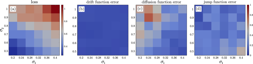
Appendix G Varying the coefficients that determine diffusion and jump functions

Here, we consider changing the two parameters $\sigma_{0},y_{0}$ in Eq. (57) of Example 4.1. With larger $\sigma_{0},y_{0}$, the trajectories generated by Eq. (57) will be subject to greater fluctuations. We use the temporally squared $W_{2}$ distance as the loss function. We vary $\sigma_{0}$ to range from 0.2 to 0.4 and vary $y_{0}$ from 0.5 to 1. We repeat our experiments 10 times, and we plot the temporally squared $W_{2}$ distance as well as the errors of the reconstructed $\hat{f},\hat{\sigma},\hat{\beta}$.

Refer to caption
Figure 4: (a) The temporally decoupled squared Wasserstein distance $\tilde{W}_{2}^{2}(\mu_{N},\hat{\mu}_{N})$. (b) the average relative errors in the reconstructed drift function $\hat{f}(x)$; (c) the average relative errors in the reconstructed diffusion function $\hat{\sigma}(x)$; (d) the average relative errors in the reconstructed jump functions $\hat{\beta}(x)$.

From Fig. 4(a), larger $\sigma_{0},y_{0}$ lead to larger $\tilde{W}_{2}^{2}(\mu_{N},\hat{\mu}_{N})$. This could be because larger $\sigma_{0},y_{0}$ lead to ground truth trajectories with larger fluctuations, rendering the underlying dynamics harder to reconstruct. Fig. 4(b) implies that the drift function can be accurately reconstructed and is insensitive to different $\sigma_{0},y_{0}$. As seen in Fig. 4(c), if $\sigma_{0}$ is small, the relative error in the reconstructed diffusion function can be well controlled around $0.1$; when $\sigma_{0}$ is larger, it is harder to reconstruct the diffusion function and the relative error in the reconstructed diffusion function $\hat{\sigma}$ will be larger. Fig. 4(d) shows that the reconstruction of the jump function $\hat{\beta}$ is not very sensitive to different values of $\sigma_{0}$ and $y_{0}$.

Appendix H Reconstructing Eq. (59) in Example 4.2 with different numbers of trajectories in the training set

Here, we carry out an additional numerical experiment of reconstructing Eq. (59) by changing the number of trajectories in the training set. We define the ground truth jump-diffusion process by the drift function $\alpha(X,t)\coloneqq r$, and the diffusion function and jump functions $\sigma(X,t)=\beta(X,t)=0.1\sqrt{|X|}$. We consider four scenarios: i) provide no prior information and reconstruct drift, diffusion, and jump functions, ii) provide the drift function $\alpha(X,t)$ as prior information and reconstruct the diffusion and jump functions, iii) provide the diffusion function $\sigma(X,t)$ as prior information and reconstruct the drift and jump functions, and iv) provide the jump function $\beta(X,t)$ as prior information and reconstruct the drift and diffusion functions.

Refer to caption
Figure 5: The reconstruction errors in the drift, diffusion, and jump functions defined in Eqs. 54 and 55 as a function of the number of trajectories $M_{s}$ when different prior information is provided. The results are averaged over 5 independent experiments. Training hyperparameters are the same as those used in Example 4.2 listed in Table 3.

As seen in Figs. 5(b-c), providing the drift function as prior information greatly boosts the efficiency of our temporally decoupled squared $W_{2}$ method allowing it to accurately reconstructing the unknown diffusion and jump functions even with as few as 100 trajectories for training. Also, even with no prior information, the errors in the reconstructed drift, diffusion, or jump function decrease when the number of trajectories in the training set increases (Figs. 5(a-c)). This indicates that even without prior information, our temporally decoupled squared $W_{2}$ method can accurately reconstruct Eq. (59) when provided a sufficient number of training trajectories.

When the diffusion or jump function is given as prior information, the errors of the reconstructed unknown functions do not decrease much as the number of trajectories for training $M_{s}$ increases. Even with the correct diffusion or jump function, different realizations of the Brownian motion or the compensated Poisson process yield very different trajectories so that providing the diffusion or jump function may provide little information in discriminating trajectories.

Appendix I Reconstructing Eq. (59) in Example 4.2 with different parameters in the diffusion and jump functions when providing the drift function

Here, given the drift function $\alpha(X,t)\coloneqq r$, we carry out an additional numerical experiment of reconstructing Eq. (59) by varying the parameters $\sigma_{0},\beta_{0}$ that determine the strength of the Brownian-type and compensated-Poisson-type noise in Eqs. (60),  (61), and  (62).

Refer to caption
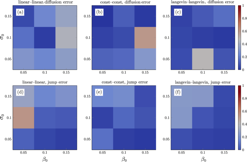
Figure 6: The reconstruction errors in the diffusion, and jump functions defined in Eqs. 54 and 55 w.r.t. the two parameters that determine the strength of noise $\sigma_{0}$ and $\beta_{0}$ in Eqs. (60),  (61), and  (62). Here, const-const indicates we are using Eq. (60) for both the diffusion and jump functions; linear-linear indicates we are using Eq. (61) for both the diffusion and jump functions; langevin-langevin indicates we are using Eq. (62) for both the diffusion and jump functions. The results are averaged over 5 independent experiments. Training hyperparameters are the same as Example 4.2 in Table 3.

Fig. 6 shows our temporally decoupled squared $W_{2}$-distance loss function can be used to accurately reconstruct the diffusion function and the jump function $\sigma(X,t),\beta(X,t)$ in Eq. (59), even when different forms of $\sigma(X,t),\beta(X,t)$ in Eqs. (60),  (61), and  (62) and different noise strengths $\sigma_{0},\beta_{0}$ are given. The average errors (averaged over all choices of $\sigma_{0},\beta_{0}$) in the reconstructed diffusion function $\hat{\sigma}$ are 0.171 (const-const), 0.217 (linear-linear), and 0.176 (langevin-langevin). The average errors (averaged over all choices of $\sigma_{0},\beta_{0}$) in the reconstructed jump function $\hat{\sigma}$ are 0.173 (const-const), 0.188 (linear-linear), and 0.184 (langevin-langevin).

Appendix J Neural Network Architecture

Here, we investigate how the neural network architecture, i.e., the number of hidden layers and the number of neurons in each layer, influence the accuracy of reconstructing the 2D jump-diffusion process (Eq. (63)). We vary only the number of hidden layers and the number of neurons per layer for the parameterized neural networks that we use to approximate the diffusion and jump functions $\bm{\sigma}$ and $\bm{\beta}$ in Eq. (63). We set the parameters to be $c_{1}=-0.5,c_{2}=-1$ and $\sigma_{0}=\beta_{0}=0.1$ in Eqs. (65) and (66), and consider 200 trajectories.

Table 4: Reconstructing the jump-diffusion process Eq. (63) when using neural networks with different numbers of hidden layers and neurons per layer to parameterize $\hat{f},\hat{\sigma}$. Other training hyperparameters are the same as those used in Table 3 of Example 4.3.
Width Layer Relative Errors in $\hat{\bm{\sigma}}$ Relative Errors in $\hat{\bm{\beta}}$ $N_{\rm repeats}$
25 3 $0.6836(\pm 0.5177)$ $0.5554(\pm 0.4024)$ 5
50 3 $0.8051(\pm 0.4756)$ $0.7413(\pm 0.3515)$ 5
100 3 $0.6376(\pm 0.3261)$ $0.5085(\pm 0.2841)$ 5
200 3 $0.6101(\pm 0.2435)$ $0.5280(\pm 0.2038)$ 5
400 3 $0.2619(\pm 0.1859)$ $0.2837(\pm 0.1961)$ 5
200 1 $0.7143(\pm 0.8451)$ $0.6178(\pm 0.2925)$ 5
200 2 $0.6984(\pm 0.4989)$ $0.6326(\pm 0.4445)$ 5
200 4 $0.7605\pm 0.3837)$ $0.6750\pm 0.2761)$ 5

From Table 4, we see that increasing the number of hidden layers and increasing the number of neurons per hidden layer can both increase the accuracy of the reconstructed $\hat{\bm{\sigma}}$ and $\hat{\bm{\beta}}$. However, with a fixed number of neurons per hidden layer (200), when the number of hidden layers in the feed-forward neural network is greater than 3, the errors in the reconstructed $\bm{\sigma}$ and $\bm{\beta}$ increase. This behavior may be due to vanishing gradients during training of deep neural networks [36]; in this case, the ResNet technique [37] can be considered if deep neural networks are used. On the other hand, using a deeper or wider network requires more memory usage and longer run times. For reconstructing Eq. (63), we find an optimal neural network architecture consisting of about three hidden layers containing $\sim 400$ neurons each. How optimal architectures evolve when reconstructing different multidimensional jump-diffusion processes requires further exploration.