TimeCMA: Towards LLM-Empowered Time Series Forecasting via Cross-Modality Alignment

Abstract.

The widespread adoption of scalable mobile sensing has led to large amounts of time series data for real-world applications. A fundamental application is multivariate time series forecasting (MTSF), which aims to predict future time series values based on historical observations. Existing MTSF methods suffer from limited parameterization and small-scale training data. Recently, Large language models (LLMs) have been introduced in time series, which achieve promising forecasting performance but incur heavy computational costs. To solve these challenges, we propose TimeCMA, an LLM-empowered framework for time series forecasting with cross-modality alignment. We design a dual-modality encoding module with two branches, where the time series encoding branch extracts relatively low-quality yet pure embeddings of time series through an inverted Transformer. In addition, the LLM-empowered encoding branch wraps the same time series as prompts to obtain high-quality yet entangled prompt embeddings via a Pre-trained LLM. Then, we design a cross-modality alignment module to retrieve high-quality and pure time series embeddings from the prompt embeddings. Moreover, we develop a time series forecasting module to decode the aligned embeddings while capturing dependencies among multiple variables for forecasting. Notably, we tailor the prompt to encode sufficient temporal information into a last token and design the last token embedding storage to reduce computational costs. Extensive experiments on real data offer insight into the accuracy and efficiency of the proposed framework.

1. Introduction

With the proliferation of scalable mobile sensing, large amounts of time series data have been collected in various domains, such as electricity (Trindade, 2015; Karatzoglidi et al., 2021), economics (McCracken and Ng, 2016), health (Lai et al., 2018), and the environment (Wu et al., 2021a). These data form the foundation for various applications (Campos et al., 2023, 2021; Schmidl et al., 2022), such as multivariate time series forecasting (MTSF), which aims to mine temporal dynamics and correlations among different variables from historical data to predict future time series (Liu et al., 2023; Cheng et al., 2023; Zhao et al., 2023). In this way, users can make decisions in advance, for example, weather forecasting makes it possible to better prepare for severe weather conditions (Hettige et al., 2024).

Existing time series forecasting methods can be roughly divided into statistical methods (Smith and Demetsky, 1997), shallow model-based methods (Zeng et al., 2023; Wu et al., 2023; Zhou et al., 2022; Nie et al., 2023), and large language model (LLM)-based methods (Jin et al., 2024a; Liu et al., 2024a; Zhou et al., 2023; Liu et al., 2024b). For statistical and shallow model-based methods, despite their success, the limited number of learnable parameters and the small-scale training data prevents them from achieving better performance (Jin et al., 2024b). Therefore, some recent advances (Zhou et al., 2023; Liu et al., 2024b) have incorporated pre-trained LLM (Radford et al., 2019, 2018) into MTSF to benefit from the high-quality embeddings learned from abundant language data, and set new state-of-the-arts on various MTSF benchmarks.

According to the types of input data, existing LLM-based methods for time series forecasting include: (1) Time series-based LLMs (Zhou et al., 2023; Liu et al., 2024b). They replace LLM’s tokenizer with a randomly initialized embedding layer to obtain the initial embeddings of the input time series data, which are then processed by the Transformer blocks for embedding enhancement. Unfortunately, the newly introduced embedding layer is still trained with limited data, and a domain gap exists between time series and language data. Therefore, the obtained time series embeddings may still be suboptimal; (2) Prompt-based LLMs (Jin et al., 2024a; Liu et al., 2024a): to tackle them, prompt-based LLMs wrap the original time series with some text descriptions to achieve the data-to-text transformation (Xue and Salim, 2023), and sequentially forward the wrapped sentences to the pre-trained tokenizer and LLM blocks to obtain high-quality embeddings. In this way, prompt-based LLMs can show better performance than time series-based methods (some evidence is included in Section 5.2).

Figure 1. Prompt-based LLMs. (a) Existing methods use LLM or deep learning models as text embedder. They calculate embeddings separately for each variable, preventing these methods from learning dependencies between multiple variables. (b) Our LLM-empowered method captures dependencies among multiple variables. A frozen LLM acts as an enhancer. The last token embeddings are stored for fast inference, while pure time series embeddings are aligned for efficient forecasting.

Although appealing performance can be achieved by prompt-based LLMs, they suffer from the data entanglement issue, as shown in Figure 1 (a). For instance, each text prompt consists of some words and the numeric in the original time series, and it would then be converted into tokens, where each token corresponds to either part of the words or time series. After that, Transformer blocks in the LLM would fuse each token with other embeddings. Specifically, word token embedding would inevitably be aggregated into time series tokens (refer to attention map in Figure 7) , they might degrade the performance, as the words information acts like noises for a forecasting task. In addition, in most existing prompt-based LLMs, each univariate time series is calculated separately for each variable, which prevents the methods from learning dependencies between multiple variables. In this paper, we aim to separate the time series information from the entangled embeddings (obtained from the prompt-based LLMs) while capturing dependencies among multiple variables for better MTSF, as depicted in Figure 1 (b).

Overall, we present an LLM-empowered framework for multivariate time series forecasting with cross-modality alignment, called TimeCMA. It includes a dual-modality encoding module with a time series encoding branch and an LLM-empowered encoding branch, a cross-modality alignment module, and a time series forecasting module. The time series encoding branch extracts relatively low-quality yet pure embeddings from historical time series data. At the same time, the LLM-empowered prompt encoding branch wraps the same time series as text prompts for obtaining high-quality yet entangled embeddings. Then, the cross-modality alignment module is designed to integrate the two groups of embeddings. Intuitively, the low-quality time series embeddings would naturally have stronger correspondences to the time series values in the entangled embeddings. Therefore, the high-quality and pure time series embeddings can be retrieved and aggregated into the low-quality time series embeddings for enhancement, leading to robust forecasting.

Nonetheless, the heavy computational burden of prompt-based LLMs leads to large training costs and quite slow inference speeds, which are mainly raised by: (i) The characteristics of multivariate time series (MTS) data: unlike with 1D prompt data (with $N$ tokens), MTS data has variable and temporal 2 dimensions (with $N$ variables and $T$ timestamps). Since self-attention is the primary component of LLM-based methods, this often results in substantial computational burdens. (ii) Repetitive computations with the frozen LLM: during training, most of existing prompt-based LLMs (Jin et al., 2024a) would perform online inference with the frozen LLM. Consequently, each training sample would be repetitively processed by the LLM in each training epoch, though the obtained embeddings remain unchanged due to the frozen parameters. Therefore, the re-training and inference time cost would be much larger.

To solve the above challenges, we further propose the last token embedding storage in the prompt encoding branch. First, the prompts are transformed MTS data and incorporate temporal information on each variable to maintain the characteristics of the MTS data. Then, we tailor a last token embedding of prompt from the frozen LLM, as the last token embedding encapsulates the most comprehensive knowledge due to the masked multi-self attention within the LLM. In this way, we condense sufficient temporal information into the last token embedding to reduce further computational costs. Moreover, we store the last token embedding to contend with the repetitive computations of frozen LLM, thereby accelerating the inference speed. Finally, the time series forecasting module decodes the aligned embeddings based on time series and last token embeddings, which captures high-quality temporal dependencies among multiple variables for future forecasting.

The major contributions are summarized as follows.

• We propose an LLM-empowered multivariate time series forecasting framework called TimeCMA, that comprises a time series branch and an LLM-empowered prompt branch in dual-modality module to capture temporal dependencies among multiple variables and to generate well-knowledge embeddings, respectively.

• We design a cross-modality alignment module to retrieve high-quality and pure time series embeddings from the knowledgeable prompt embeddings for more effective multivariate time series forecasting.

• TimeCMA stores the last token embeddings of the prompt to facilitate time series forecasting, which largely reduces computational costs and accelerates the inference speed.

• Extensive experiments on eight real datasets demonstrate the accuracy and efficiency of the proposed TimeCMA framework.

Figure 2. TimeCMA framework overview.

2. Related Work

Time series forecasting (Wu et al., 2021b; Zhao et al., 2023; Qiu et al., 2024) attracts increasing interest due to the increasing availability of time series data and rich downstream applications in real-world scenarios, such as human mobility prediction (Xue et al., 2022) and financial forecasting (Niu et al., 2020).

In this paper, we focus on multivariate time series forecasting, whereas recent methods focus more on designing various deep learning-based models (Wu et al., 2021b; Zhao et al., 2023; Cheng et al., 2023). Transformers have achieved excellent performance due to their powerful learning capabilities (Zhou et al., 2022; Liu et al., 2022). However, the self-attention in Transformers introduces high computational overhead and memory consumption. To improve efficiency, simplified Transformer-based models, e.g., Reformer (Kitaev et al., 2020), Informer (Zhang et al., 2021), CrossFormer (Zhang and Yan, 2023), and iTransformer (Liu et al., 2023), have been developed to reduce the computational overhead from the input or network architecture perspective. Nonetheless, these methods are often trained for a specific domain while failing to adapt to various scenarios and thus suffer from scalability.

Large Language Models (LLMs) have seen significant advancement in natural language processing and computer vision. Recent work has shown that LLMs present a significant potential for time series analysis (Jin et al., 2024b). In the early stage, a line of studies, such as AuxMobLCast (Xue et al., 2022) and PromptCast (Xue and Salim, 2023), utilize LLMs for general human mobility forecasting through prompting techniques. Subsequently, more advanced approaches emerge, involving fine-tuning based LLMs for specific downstream tasks (Zhou et al., 2023; Liu et al., 2024b). Later, several works have shown that aligning time series features with LLM representations can enhance the model’s understanding of temporal patterns (Gruver et al., 2023; Cao et al., 2024; Jin et al., 2024a; Liu et al., 2024a). These alignments involve mapping time series features to the corresponding linguistic elements within the model (Jin et al., 2024b).

However, existing LLM-based methods face issues such as slow inference speed and large memory usage. In contrast to these methods, we leverage the last token embedding of text prompts driven by LLM to align time series embeddings and develop an efficient LLM-empowered cross-modality alignment framework for multivariate time series forecasting.

3. Preliminaries

In this section, we present some definitions used throughout this paper and then formulate the problem of multivariate time series forecasting.

Definition 3.1 (Multivariate Time Series).

Multivariate time series is denoted as $\mathbf{X}=\left\{\mathbf{x}_{1},\ldots,\mathbf{x}_{L}\right\}\in\mathbb{R}^{L\times N}$, where $T$ is the number of time steps and $N$ is the number of variables. Each $\mathbf{x}_{l}$ is a $N$-dimensional vector, which indicates several $N$ variables (e.g., load or temperature) at time step $l$, where we use $v_{i}$ to denote the value of $i$-$th$ variable.

Definition 3.2 (Prompt).

We convert the original time series $\mathbf{X}\in\mathbb{R}^{L\times N}$ into $N$ prompts $\mathbf{P}_{S}=\left\{\mathbf{p}_{1},\ldots,\mathbf{p}_{N}\right\}\in\mathbb{R}^{S\times N}$ along with variables according to a template, which is as shown in Figure 2. In $\mathbf{P}_{S}$, each prompt $\mathbf{p}_{i}$ has $S$ elements containing text and numeric values. In the template, the $<\textit{italic}>$ elements represent time information, such as timestamps and frequency. The $<{\color[rgb]{0.90234375,0.61328125,0.6328125}color}>$ elements denote time series values. The overall trend within a prompt is quantified by the total trend value $\Delta_{T}$, defined as:

(1) $$\Delta_{T}=\sum_{i=1}^{T-1}\delta v_{i},$$

where $\delta v_{i}=v_{i+1}-v_{i}$ represents the incremental change between consecutive measurements.

Problem Definition. Given an observation in a multivariate time series $\mathbf{x}_{t}\in\mathbb{R}^{N}$, where $t$ is a time step and $N$ indicates the number of variables. Our goal is to learn a function using historical multivariate time series $\mathbf{X}_{T}=\{\mathbf{x}_{t-T+1:t}\}\in\mathbb{R}^{T\times N}$ to forecast future time series $\widehat{\mathbf{X}}_{M}=\left\{\widehat{\mathbf{x}}_{t+1:t+M}\right\}\in\mathbb{R}^{M\times N}$ over $M$ timesteps.

4. Methodology

In this section, we propose TimeCMA, an LLM-empowered framework for multivariate time series forecasting with cross-modality alignment. We first provide an overview of the framework and then provide specifics on each module in the framework.

4.1. Framework Overview

The framework consists of three major modules: dual-modality encoding, cross-modality alignment, and time series forecasting, as shown in Figure 2.

Dual-Modality Encoding. In this module, we design two complicated encoding branches, including a time series encoding branch and an LLM-empowered encoding branch, aiming at effective learn embeddings for input time series and text prompts, respectively. Through this module, we can separate the time series and text prompt embeddings to enhance more effective feature learning.

Time Series Encoding Branch. The time series encoding branch consists of an inverted embedding layer and a time series encoder, that is used in Pre-LN Transformer (Xiong et al., 2020). The inverted embedding layer embeds the original time series into a single vector to capture its long-term temporal dependencies. We then input the embedded vector into the encoder, aiming to capture the complex temporal dependencies between multiple variables.

LLM-Empowered Encoding Branch. The LLM-empowered encoding branch comprises a pre-trained LLM and a prompt encoder with the same architecture as that in time series encoder. The frozen LLM extracts high-quality prompt embeddings with the sufficient information extracted from the original times series, and the prompt encoder enhances these embeddings between multiple variables.

Cross-Modality Alignment. In this module, we propose a novel cross-modality alignment to aggregate the learned time series and prompt embeddings. The purpose of the cross-modality method is to retrieve high-quality time series embeddings from prompt embeddings.

Time Series Forecasting. In this module, we utilize the decoder, which is similar to that in Pre-LN Transformer to decode the aligned time series embeddings, which are learned from the cross-modality alignment module. The decoder aims to facilitate further long-term temporal dependencies learning between multiple variables. Finally, the decoded embeddings are input into a projection function for future forecasting.

Next, we will elaborate on the technical details of each module, respectively.

4.2. Dual-Modality Encoding

4.2.1. Time Series Encoding Branch

Previous time series forecasters regard multiple variates simultaneously as the temporal token, further embedding multiple variables of the same timestamp (Zhou et al., 2023). These methods frequently exhibit suboptimal performance, as they conflate the representations of multiple unrelated variables. Later, channel independence has been proposed to address this problem. However, due to the longer training times associated with channel independence, it is unsuitable for time series data involving more variables. Additionally, channel independence overlooks the dependencies between multiple variables, making it challenging to achieve good performance on data with closely related variables. In this section, the time series branch employs the inverted embedding (Liu et al., 2023, 2024b), which defines the entire time series of a variable token.

Embedding. Given the time series data $\mathbf{X}_{T}\in\mathbb{R}^{T\times N}$, the inverted embedding aims to convert $\mathbf{X}_{T}$ into learnable matrices to capture the temporal dependencies of variables. Specifically, the $\mathbf{X}_{T}$ is normalized to have zero mean and unit standard deviation via reversible instance normalization to mitigate the time series distribution shift (Kim et al., 2022). Then, the normalized $\mathbf{X}_{T}$ is embedded by a linear layer:

(2) $$\mathbf{H}_{T}=\mathbf{W}_{e}\mathbf{X}_{T}+\mathbf{b}_{e},$$

where $\mathbf{H}_{T}=\left\{\mathbf{h}_{1},\ldots,\mathbf{h}_{T}\right\}\in\mathbb{R}^{C\times N}$ is the output of the embedding layer. $C$ indicates the hidden dimension of the embedded time series. $\mathbf{W}_{e}$ and $\mathbf{b}_{e}$ are the learnable parameters.

Time Series Encoder. The time series embeddings $\mathbf{H}_{T}$ are fed into a time series encoder $\mathit{TSEncoder(\cdot)}$. Inspired by the structure of LLM in Figure 2, we apply layer normalization first in the encoder, meaning it occurs before both the multi-head attention and feed-forward layers. Compared with the original Transformer, the Pre-LN Transformer has the advantages of being more stable and converging faster (Huang et al., 2023). In $\mathit{TSEncoder(\cdot)}$, the embeddings $\mathbf{H}_{T}^{i}$ undergo $i_{\text{th}}$ layer normalization $\mathit{LN}(\cdot)$:

(3) $$\widetilde{\mathbf{H}}_{T}^{i} =\mathit{LN}(\mathbf{H}^{i}_{T}),$$

(4) $$\mathit{LN}(\mathbf{H}^{i}_{T}) =\gamma\odot\frac{\mathbf{H}^{i}_{T}-\mu}{\sigma}+\beta,$$

where $\widetilde{\mathbf{H}}^{i}_{T}$ represents the intermediate embedding after the $i_{\text{th}}$ layer normalization. $\gamma$ and $\beta$ are learnable scaling and translation parameters. $\mu$ and $\sigma$ represent the mean and standard deviation, respectively. $\odot$ denotes element-wise multiplication.

Then, they are processed by the multi-head self-attention mechanism, denoted as $\mathit{MHSA}(\cdot)$. The output, $\overline{\mathbf{H}}_{T}^{i}$, is combined with $\mathbf{H}_{T}^{i}$ through a residual connection:

(5) $$\overline{\mathbf{H}}_{T}^{i} =\mathit{MHSA}(\widetilde{\mathbf{H}}_{T}^{i})+\mathbf{H}^{i}_{T},$$

(6) $$\mathit{MHSA}(\mathbf{H}^{i}_{T}) =\rho_{o}(\mathit{Attention}(\rho_{q}\mathbf{H}^{i}_{T},\rho_{k}\mathbf{H}^{i}_{T},\rho_{v}\mathbf{H}^{i}_{T})),$$

(7) $$\mathit{Attention}(\mathbf{H}^{i}_{T}) =\mathit{softmax}\left(\frac{\mathbf{H}^{i}_{T}\mathbf{H}^{iT}_{T}}{\sqrt{d_{k}}}\right)\mathbf{H}^{i}_{T},$$

where $\mathbf{\overline{H}}^{i}_{T}$ is output of the $i_{\text{th}}$ layer after the $\mathit{MHSA}(\cdot)$. $\rho_{o}$, $\rho_{q}$, $\rho_{k}$, and $\rho_{v}$ are the linear projections.

Followed by another $\mathit{LN}(\cdot)$. The normalized $\grave{\mathbf{H}}_{T}^{i+1}$ are then passed through a feed-forward network $\mathit{FFN}(\cdot)$ of fully connected layers that further process the embeddings, then combined with the $\overline{\mathbf{H}}_{T}^{i}$ through another residual connection. The process can be formulated:

(8) $$\grave{\mathbf{H}}_{T}^{i+1} =\mathit{LN}(\overline{\mathbf{H}}^{i}_{T}),$$

(9) $$\mathbf{H}_{T}^{i+1} =\mathit{FFN}(\mathit{LN}(\grave{\mathbf{H}}^{i}_{T}))+\overline{\mathbf{H}}^{i}_{T},$$

(10) $$\mathit{FFN}(\overline{\mathbf{H}}^{i}_{T}) =\max(0,\mathbf{W}_{1}\mathbf{H}^{i}_{T}+\mathbf{b}_{1})\mathbf{W}_{2}+\mathbf{b}_{2},$$

where $\mathbf{\grave{H}}^{i}_{T}$ represents the intermediate embedding of the $i_{\text{th}}$ layer after the second $\mathit{LN}(\cdot)$. $\mathbf{H}^{i+1}_{T}$ symbolizes the output of $\mathit{TSEncoder(\cdot)}$.

4.2.2. LLM-Empowered Encoding Branch

Pre-trained LLMs learn from all input tokens, making them much more sample-efficient than encoder-only models given the same training data (BehnamGhader et al., 2024). In this study, we selected GPT2 as the pre-trained LLM to generate the prompt embeddings for enhancing the time series embeddings. The pre-trained LLM comprises a GPT2 tokenizer and a GPT2 model.

Figure 3. LLM structure.

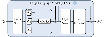
Pre-trained LLM. The GPT2 tokenizer is responsible for converting prompt input $\mathbf{P}_{S}\in\mathbb{R}^{S\times N}$ into a series of token IDs $\mathbf{P}_{G}\in\mathbb{R}^{G\times N}$, where $G$ represents the token ID number in a prompt. Subsequently, these prompt tokens are fed into the GPT2 model to generate prompt embeddings. The forward process is as follows:

(11) $$\overline{\mathcal{P}}_{G}^{i} =\mathit{MMSA}(\mathit{LN}(\mathbf{P}^{i}_{G}))+\mathbf{P}^{i}_{G},$$

(12) $$\mathcal{P}_{G}^{i+1} =\mathit{FFN}(\mathit{LN}(\overline{\mathcal{P}}^{i}_{G}))+\overline{\mathcal{P}}^{i}_{G},$$

(13) $$\mathit{MMSA}(\mathbf{P}^{i}_{G}) =\phi_{o}(\mathit{Attention}(\phi_{q}\mathbf{P}^{i}_{G},\phi_{k}\mathbf{P}^{i}_{G},\phi_{v}\mathbf{P}^{i}_{G})),$$

where $\mathcal{\overline{P}}^{i}_{G}\in\mathbb{R}^{G\times N\times E}$ represents the intermediate representation of the $i_{\text{th}}$ layer after applying the $\mathit{MMSA}(\cdot)$ and the $\mathit{LN}(\cdot)$. $E$ denotes the hidden dimension of the GPT2. $\phi_{o}$, $\phi_{q}$, $\phi_{k}$, and $\phi_{v}$ are the linear projections. $\mathcal{P}^{i+1}_{G}\in\mathbb{R}^{G\times N\times E}$ symbolizes the output embeddings of the GPT2 model .

Last Token Embedding Storage. Recent studies have verified that not all tokens are equally important for language model training (Lin et al., 2024; BehnamGhader et al., 2024). As depicted in Figure 3, the last token in a prompt holds the most comprehensive knowledge (shown in blue cubes) due to the masked multi-self attention within the LLM. Specifically, the representation of the last token at position $G$ is influenced exclusively by the representations of its previous tokens at positions $\{1,2,\cdots,G-1\}$. Therefore, we store the well-trained last token embeddings $\mathbf{L}_{N}=\left\{\mathbf{l}_{1},\ldots,\mathbf{l}_{N}\right\}\in\mathbb{R}^{N\times E}$ from the $\mathcal{P}^{i+1}_{G}\in\mathbb{R}^{G\times N\times E}$, to reduce computational cost. To maintain consistent sample embedding lengths under a variable, we repeatedly append the last token as padding until the number of tokens in the variable is the same for convenient storage.

Prompt Encoder. We define prompt encoder as $\mathit{PromptEncoder(\cdot)}$. Its structure follows the decoder in Pre-LN Transformer, identical to $\mathit{TSEncoder(\cdot)}$. We denote the output of $\mathit{PromptEncoder(\cdot)}$ as $\overline{\mathbf{L}}_{N}$.

4.3. Cross-Modality Alignment

To aggregate the dual modality features, we design a novel cross-modality alignment module to align time series and prompt embeddings, i.e., $\overline{\mathbf{H}}_{C}$ and $\overline{\mathbf{L}}_{N}$. It aims at using relatively low-quality time series embeddings $\mathbf{H}_{T}$ to retrieve relevant high-quality embeddings $\overline{\mathbf{H}}_{C}$ from prompt embeddings $\overline{\mathbf{L}}_{N}$.

First, we employ three linear layer $\psi_{q},\psi_{v},\psi_{k}$ to transform $\overline{\mathbf{H}}_{T}$ and $\overline{\mathbf{L}}_{N}$ to three compact embeddings: $\psi_{q}(\overline{\mathbf{H}}_{T})$, $\psi_{v}(\overline{\mathbf{L}}_{N})$, and $\psi_{k}(\overline{\mathbf{L}}_{N})$. Then, we compute the channel-wise similarity matrix $\mathbf{M}_{T}\in\mathbb{R}^{C\times E}$ by matrix multiplication followed by softmax:

(14) $$\mathbf{M}_{T}=\mathit{F}_{\text{softmax}}\left(\psi_{q}\left(\overline{\mathbf{H}}_{T}\right)\otimes\psi_{k}\left(\overline{\mathbf{L}}_{N}\right)\right),$$

where $\otimes$ is element-wise product.

We aggregate the channel-wise embeddings by restoring the channel dimension by the matrix multiplication of $\psi_{v}(\overline{\mathbf{L}}_{N})$ and $\overline{\mathbf{M}}_{T}$. Then, linear layer $\omega^{c}$ is applied to transform the size of the above feature maps to that of $\overline{\mathbf{H}}_{T}$. Finally, we get the output by adding $\overline{\mathbf{H}}_{T}$ to it by matrix addition:

(15) $$\overline{\mathbf{H}}_{C}=\omega^{c}\left(\psi_{v}\left(\overline{\mathbf{L}}_{N}\right)\otimes\mathbf{M}_{T}\right)+\overline{\mathbf{H}}_{T},$$

where $\overline{\mathbf{H}}_{C}\in\mathbb{R}^{C\times N}$.

Through cross-modality alignment, we transfer the knowledge learned from the powerful pre-trained LLM into time series embeddings, which thus improves the model performance.

4.4. Time Series Forecasting

We design a time series forecasting module including a temporal decoder and a projection function. In particular, we input the aggregated features $\overline{\mathbf{H}}_{C}$ into temporal decoder $\mathit{TemporalDecoder(\cdot)}$ to map the latent embeddings into the original data space. Finally, we use a projection function based on feed-forward networks for prediction.

The temporal decoder is based on Pre-LN Transformers. Specifically, we first feed the aggregated features $\overline{\mathbf{H}}_{C}$ into a layer normalization layer $LN(\cdot)$ to obtain normalized embeddings $\widetilde{\mathbf{H}}_{C}^{i}$. Then, we employ a masked multi-head self-attention layer $MMSA(\cdot)$ with residual connection to obtain $\overline{\mathbf{H}}_{C}^{i}$. Subsequently, $\overline{\mathbf{H}}_{C}^{i}$ is fed to a layer normalization $LN(\cdot)$ followed by a multi-head cross-attention layer $MHCA(\cdot)$, which can be formulated as follows,

(16) $$\mathit{MHSA}(\mathbf{H}^{i}_{C})=\varsigma_{o}(\mathit{Attention}(\varsigma_{q}\mathbf{H}^{i}_{C},\varsigma_{k}\mathbf{H}^{i}_{C},\varsigma_{v}\mathbf{H}^{i}_{C})),$$

where $\varsigma_{o}$, $\varsigma_{q}$, $\varsigma_{k}$, and $\varsigma_{v}$ are the linear projections. In addition, we apply the residual connection to obtain the output $\overline{\mathbf{H}}_{C}^{i}$ of $\mathit{TemporalDecoder(\cdot)}$.

(17) $$\overline{\mathbf{H}}_{C}^{i}=\mathit{MHCA}(\widetilde{\mathbf{H}}_{C}^{i})+\mathbf{H}^{i}_{C}.$$

Finally, the learned features $\overline{\mathbf{H}}_{C}^{i}$ are input into a projection function for future prediction. It can be formulated as follows.

(18) $$\widehat{\mathbf{X}}_{M}=\mathbf{W}_{p}\mathbf{H}_{C}+\mathbf{b}_{p},$$

where $\widehat{\mathbf{X}}_{M}\in\mathbb{R}^{M\times N}$ represents the projected forecasts. $\mathbf{W}_{p}$ and $\mathbf{b}_{p}$ are the learnable parameters. Finally, we normalize the $\widehat{\mathbf{X}}_{M}$.

4.5. Overall Objective Function

The final loss of TimeCMA contains two parts: a prediction loss $L_{pre}$ and a regularization loss $L_{reg}$. We combine them together and the overall loss is as follows,

(19) $$L_{task}=L_{pre}+\lambda L_{reg},$$

where $\lambda$ is a weight to trade off the prediction and regularization losses. Specifically, we use Mean Squared Error (MSE) as the prediction loss, which is formulated as follows,

(20) $$L_{pre}=\frac{1}{\mathcal{M}}\sum_{M=1}^{\mathcal{M}}|\mathbf{\widehat{X}}_{M}-\mathbf{X}_{M}|,$$

where $\mathcal{M}$ is the training sample size. In addition, we use L2 regularization  (Hastie et al., 2009) as the regularization loss $L_{reg}$.

Table 1. Statistics of time series and prompt.

Dataset	Dim	Frequency	Instance	Prompt Token	Split
ETTm1	7	15 min	57,600	483	6:2:2
ETTm2	7	15 min	57,600	493	6:2:2
ETTh1	7	1 hour	14,400	444	6:2:2
ETTh2	7	1 hour	14,400	505	6:2:2
ECL	321	1 hour	26,304	369	7:1:2
FRED-MD	107	1 month	728	230	7:1:2
ILI	7	1 week	966	232	7:1:2
Weather	21	10 min	52,696	508	7:1:2

5. Experiments

Table 2. Forecasting performance comparisons. The input sequence length is configured as follows: 36 for the Illness and FRED-MD datasets and 96 for others. Predictive lengths vary based on the dataset, set to {24, 36, 48, 60} for Illness and FRED-MD datasets, and {96, 192, 336, 720} for others. Note that we bold the best performance and underline the second best performance.

Models		TimeCMA (Ours)		Time-LLM 2024		UniTime 2024		OFA 2023		iTransformer 2024		PatchTST 2023		TimesNet 2023		Dlinear 2023		FEDformer 2022
Metric		MSE	MAE	MSE	MAE	MSE	MAE	MSE	MAE	MSE	MAE	MSE	MAE	MSE	MAE	MSE	MAE	MSE	MAE
ETTm1	96	0.317	0.359	0.356	0.382	0.322	0.363	0.335	0.369	0.334	0.368	0.344	0.373	0.338	0.375	0.345	0.372	0.379	0.419
	192	0.364	0.383	0.388	0.393	0.366	0.387	0.374	0.385	0.377	0.391	0.367	0.386	0.374	0.387	0.380	0.389	0.426	0.441
	336	0.403	0.405	0.419	0.414	0.398	0.407	0.407	0.406	0.426	0.420	0.392	0.407	0.410	0.411	0.413	0.413	0.445	0.459
	720	0.469	0.445	0.476	0.444	0.454	0.440	0.469	0.442	0.491	0.459	0.464	0.442	0.478	0.450	0.474	0.453	0.543	0.490
	Ave	0.388	0.398	0.410	0.408	0.385	0.399	0.396	0.401	0.407	0.410	0.392	0.402	0.400	0.406	0.403	0.407	0.448	0.452
ETTm2	96	0.177	0.259	0.185	0.272	0.183	0.266	0.190	0.275	0.180	0.264	0.177	0.260	0.187	0.267	0.193	0.292	0.203	0.287
	192	0.243	0.303	0.253	0.315	0.251	0.310	0.253	0.313	0.250	0.309	0.246	0.305	0.249	0.309	0.284	0.362	0.269	0.328
	336	0.307	0.342	0.314	0.351	0.319	0.351	0.321	0.360	0.311	0.348	0.305	0.343	0.321	0.351	0.369	0.427	0.325	0.366
	720	0.409	0.401	0.411	0.405	0.420	0.410	0.411	0.406	0.412	0.407	0.410	0.405	0.408	0.403	0.554	0.522	0.421	0.415
	Ave	0.284	0.326	0.291	0.336	0.293	0.334	0.294	0.339	0.288	0.332	0.285	0.328	0.291	0.333	0.350	0.401	0.305	0.349
ETTh1	96	0.383	0.398	0.404	0.414	0.397	0.418	0.398	0.424	0.386	0.405	0.404	0.413	0.384	0.402	0.386	0.400	0.376	0.419
	192	0.433	0.434	0.442	0.435	0.434	0.439	0.449	0.427	0.441	0.436	0.454	0.430	0.434	0.429	0.437	0.432	0.420	0.448
	336	0.458	0.448	0.473	0.451	0.468	0.457	0.492	0.466	0.487	0.458	0.497	0.462	0.491	0.469	0.481	0.459	0.459	0.465
	720	0.464	0.465	0.469	0.470	0.469	0.477	0.487	0.483	0.503	0.491	0.496	0.481	0.521	0.500	0.519	0.516	0.506	0.507
	Ave	0.440	0.436	0.447	0.443	0.442	0.448	0.457	0.450	0.454	0.447	0.463	0.449	0.458	0.450	0.456	0.452	0.440	0.460
ETTh2	96	0.292	0.343	0.295	0.345	0.296	0.345	0.312	0.360	0.297	0.349	0.312	0.358	0.340	0.374	0.333	0.387	0.358	0.397
	192	0.377	0.395	0.381	0.397	0.374	0.394	0.387	0.405	0.380	0.400	0.397	0.408	0.402	0.414	0.477	0.476	0.429	0.439
	336	0.417	0.434	0.419	0.429	0.415	0.427	0.424	0.437	0.428	0.432	0.435	0.440	0.452	0.452	0.594	0.541	0.496	0.487
	720	0.426	0.443	0.425	0.442	0.425	0.444	0.433	0.453	0.427	0.445	0.436	0.449	0.462	0.468	0.831	0.657	0.463	0.474
	Ave	0.378	0.403	0.380	0.403	0.378	0.403	0.389	0.414	0.383	0.407	0.395	0.414	0.414	0.427	0.559	0.515	0.437	0.449
ECL	96	0.143	0.241	0.172	0.265	0.196	0.287	0.197	0.290	0.148	0.240	0.186	0.269	0.168	0.272	0.197	0.282	0.193	0.308
	192	0.162	0.259	0.182	0.279	0.199	0.291	0.201	0.292	0.162	0.253	0.190	0.273	0.184	0.289	0.196	0.285	0.201	0.315
	336	0.169	0.261	0.195	0.288	0.214	0.305	0.217	0.309	0.178	0.269	0.206	0.290	0.198	0.300	0.209	0.301	0.214	0.329
	720	0.220	0.315	0.233	0.320	0.254	0.335	0.253	0.339	0.225	0.317	0.247	0.322	0.220	0.320	0.245	0.333	0.246	0.355
	Ave	0.174	0.269	0.195	0.288	0.216	0.306	0.217	0.308	0.178	0.270	0.207	0.289	0.192	0.295	0.212	0.300	0.214	0.327
FRED-MD	24	22.702	0.864	27.285	0.875	31.178	0.931	28.317	0.947	28.017	0.893	35.777	1.014	43.268	1.266	37.898	1.070	66.09	1.623
	36	41.792	1.169	48.730	1.172	54.172	1.223	59.520	1.306	50.837	1.274	61.034	1.345	69.514	1.533	71.047	1.477	94.359	1.863
	48	64.364	1.459	73.494	1.460	83.836	1.518	74.808	1.516	78.018	1.793	93.482	1.667	89.913	1.742	118.579	2.002	129.798	2.135
	60	77.792	1.611	108.221	1.758	118.429	1.830	83.613	1.641	90.212	1.693	133.444	2.011	116.187	1.976	156.844	2.221	173.616	2.435
	Ave	51.662	1.275	64.433	1.316	75.771	1.465	61.565	1.353	61.771	1.413	80.934	1.509	79.721	1.629	96.092	1.693	115.966	2.014
ILI	24	1.996	0.917	2.383	1.004	2.346	0.954	2.732	1.100	2.347	1.731	2.335	0.989	2.317	0.934	2.398	1.040	3.228	1.260
	36	1.946	0.940	2.390	0.993	1.998	0.912	2.664	1.063	2.468	0.998	2.561	1.035	1.972	0.920	2.646	1.088	2.679	1.080
	48	1.940	0.923	2.394	1.003	1.979	0.912	2.617	1.041	2.489	1.016	2.465	1.022	2.238	0.940	2.614	1.086	2.622	1.078
	60	2.114	0.926	2.562	1.049	2.109	0.938	2.478	1.035	2.471	1.065	2.189	0.997	2.027	0.928	2.804	1.146	2.857	1.157
	Ave	1.999	0.927	2.432	1.012	2.108	0.929	2.623	1.060	2.444	1.203	2.388	1.011	2.139	0.931	2.616	1.090	2.847	1.144
Weather	96	0.167	0.211	0.198	0.235	0.171	0.214	0.203	0.244	0.174	0.214	0.177	0.218	0.172	0.220	0.196	0.255	0.217	0.296
	192	0.212	0.253	0.240	0.269	0.217	0.254	0.247	0.277	0.221	0.254	0.222	0.259	0.219	0.261	0.237	0.296	0.276	0.336
	336	0.270	0.294	0.295	0.308	0.274	0.293	0.297	0.311	0.278	0.296	0.277	0.297	0.280	0.306	0.283	0.335	0.339	0.380
	720	0.350	0.348	0.368	0.353	0.351	0.343	0.368	0.356	0.358	0.349	0.352	0.347	0.365	0.359	0.345	0.381	0.403	0.428
	Ave	0.250	0.276	0.275	0.291	0.253	0.276	0.279	0.297	0.258	0.279	0.257	0.280	0.259	0.287	0.265	0.317	0.309	0.360

5.1. Experimental Setup

5.1.1. Datasets.

We conduct our experiments with eight scalable datasets, which include ETTm1, ETTm2, ETTh1, ETTh2 (Zeng et al., 2023), ECL (Asuncion and Newman, 2007), FRED-MD (McCracken and Ng, 2016), ILI, and Weather (Wu et al., 2021a). We removed variables with missing values in the FRED-MD dataset (Qiu et al., 2024). Prompts are derived from the original time series data. We calculate the average token number of a prompt for each dataset as the Prompt Token. Details of these datasets are provided in Table 1.

5.1.2. Baselines and evaluation metrics.

We select eight forecasting methods as our baselines with four categorizations: (1) LLM-based methods, i.e., Time-LLM (Jin et al., 2024a), UniTime (Liu et al., 2024a), and OFA (Zhou et al., 2023). Time-LLM and UniTime are prompt-based LLMs, while OFA is the time series-based LLM. (2) Transformer-based methods, i.e., iTransformer (Liu et al., 2023), PatchTST (Nie et al., 2023), and FEDformer (Zhou et al., 2022). (3) Linear-based model, i.e., Dlinear (Zeng et al., 2023). (4) CNN-based model, i.e., TimesNet (Wu et al., 2023). The evaluation metrics contain mean square error (MSE) and mean absolute error (MAE) (Eichinger et al., 2015).

5.1.3. Implementation Details.

To ensure fairness and conserve general computational cost for MTSF, all LLM-based methods use GPT-2 as the backbone. Most importantly, the test batch size is set to 1 for all methods to guarantee consistency in the testing phase (Qiu et al., 2024). The lookback window length is fixed at 36 for the ILI and FRED-MD, and 96 for the others. We train our method using the AdamW optimizer and select the trained model with the lowest average validation loss for testing. Each experiment is repeated at least three times with different seeds on an NVIDIA A100 GPU.

5.2. Main Results

Our main results are shown in Table 2, where TimeCMA outperforms all baselines in most cases and significantly in most of them. (1) LLM-based methods perform better than traditional methods. These results verify our motivation to use LLMs for time series forecasting. (2) Inverted embedding is essential for datasets with more variables. TimeCMA performs better on datasets with more variables, such as ECL, FRED-MD, and Weather. iTransformer shows similar results since it also takes an inverted view of the time series. While other methods perform better on datasets with fewer variables, TimeCMA still outperforms those methods. (3) Prompt-based LLMs outperform time series-based LLM. The prompt-based LLM such as TimeCMA has approximately 19.1% better performance in terms of MSE and 11.3% better performance in terms of MAE compared to the time series-based LLM OFA. The improvement is attributed to the enhanced time series embeddings through prompt embeddings, which are not used in OFA. Among prompt-based LLMs, TimeCMA is the best, followed by UniTime. Compared to UniTime, TimeCMA achieves an average improvement of approximately 13.9% in MSE and 12.6% in MAE across all datasets. It is noteworthy that UniTime is trained on all datasets and tested a dataset, while TimeCMA is trained on a dataset and tested on a dataset. Combining this with the subsequent experimental results in Table 4. Additionally, TimeCMA performs better than Time-LLM. This is because our prompt can learn better temporal trends than the prompt in Time-LLM, and the cross-modality alignment module is superior to direct concatenation embeddings in the Time-LLM.

5.3. Ablation Studies

5.3.1. Results of model design.

To better understand the effectiveness of the model designs in TimeCMA, we construct five variants of the TimeCMA and conduct ablation studies across ILI and FRED-MD datasets. The experimental results are average values from all predictive lengths, summarized in Figure 4. These results demonstrate the importance of each component in achieving optimal performance.

(a) ILI.

(b) FRED-MD.

Figure 4. Ablation study of model design. We report the average value over all predictive lengths.

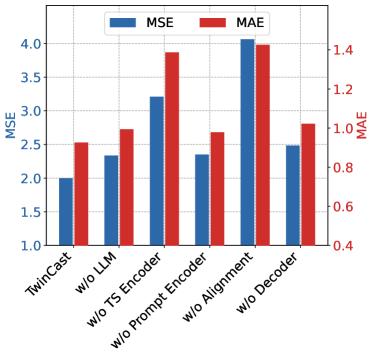
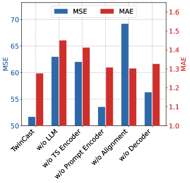
The results in Figure 4 indicate that ablating either pre-trained LLM or cross-modality alignment hurts knowledge transfer in the LLM for time series forecasting. The ablation of pre-trained LLM ($w/o~{}LLM$) signifies that the TS-LLM branches have better prediction results than only the TS branch. In the absence of time series encoder ($w/o~{}TS~{}Encoder$), the degradation results indicate that extracting better time series embeddings is fundamental for forecasting. We find that removing the prompt encoder has the least impact, as the previous pre-trained LLM captures the dependencies between variables, and the prompt encoder’s role is to better prepare for the subsequent cross-modality alignment. The variant with the most significant impact on the model is $w/o~{}alignment$, which means correctly aligning the time series and text modalities is crucial to retrieving time series embeddings from prompt embeddings. Furthermore, $w/o~{}Decoder$ shows that decoding long-term temporal dependencies between multiple variables is also crucial.

Figure 5. Examples of different prompt designs. The example of Prompt 5 is depicted in Figure 2.

(a) ILI.

(b) FRED-MD.

Figure 6. Forecasting performance of prompt designs.

5.3.2. Results of prompt design.

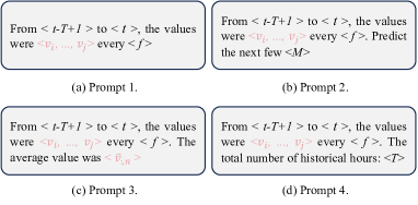
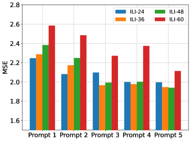
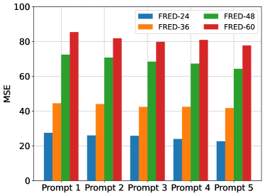
We design five prompts in this study, as illustrated in Figures 2 and 5. First, we extract time and value information directly in Prompt 1. Since we use the last token in the prompt to assist in time series forecasting, we carefully design it so that its last token is a numerical value to contain more time-related information. Prompt 2 contains the forecasting guidance for the next few timestamps. We summarize the average value of a variable over a given period in Prompt 3. Historical time information is derived in Prompt 4. Finally, we calculate the trend value in Prompt 5. The forecasting performance of different prompt designs is shown in Figure 6. We observe that prompts where the last token is a numerical value generally have better prediction performance, such as Prompts 3, 4, and 5. Among these numeric last-token prompts, Prompt 5 is the best. The Prompt 5 abstracts the time series trends, which is useful for forecasting. The second best is prompt 3, which averages the time series but may introduce noise, making the prediction less optimal. Following this is Prompt 2, which emphasizes the historical time information. Compared with time, values are more important for forecasting.

5.4. Zero-shot forecasting

In this section, we delve into the transferability of our TimeCMA and LLM baselines from the source domains to the target domains. Specifically, we train the models on ETTh1, ETTh2, and ILI datasets. Then, we assess their performance in both intra-domain transfer and inter-domain transfer scenarios through zero-shot forecasting. This testing is conducted on ETTh1 and ETTh2. The results are shown in Table 3. In these experiments, the parameters in LLM are frozen in TimeCMA and Unitime, unfrozen in UniTime, and partially frozen in OFA.

Table 3. Zero-shot forecasting on intra-domain and inter-domain scenarios.

Parameters in LLM	Frozen				Unfrozen		Partial Frozen
Method	TimeCMA		Time-LLM		UniTime		OFA
Metric	MSE	MAE	MSE	MAE	MSE	MAE	MSE	MAE
ETTh1 $\longrightarrow$ ETTh2	0.298	0.341	0.300	0.346	0.287	0.346	0.301	0.349
ETTh2 $\longrightarrow$ ETTh1	0.518	0.483	0.522	0.479	0.521	0.487	0.381	0.394
ILI $\longrightarrow$ ETTh1	0.709	0.556	0.802	0.572	0.847	0.603	0.923	0.673
ILI $\longrightarrow$ ETTh2	0.354	0.388	0.404	0.417	0.443	0.445	0.231	0.333

The table illustrates that TimeCMA consistently outperforms the baselines across most cases, especially in inter-domain scenarios, affirming the effectiveness of our prompt design and inter-domain alignment. OFA is the second best based on its partial frozen parameters. UniTime and Time-LLM are better at inter-domain transfer.

5.5. Model Analysis

5.5.1. Model Efficiency Analysis.

Table 4. Efficiency analysis of TimeCMA and LLM-based baselines.

Dataset	ETTh1-96			ILI-24			FRED-MD-24
Metric	Param. (M)	Mem. (MiB)	Speed(s/iter)	Param. (M)	Mem. (MiB)	Speed(s/iter)	Param. (M)	Mem. (MiB)	Speed(s/iter)
TimeCMA	17.030	814	0.120	16.237	622	0.031	17.269	744	0.023
Time-LLM	304.830	23944	9.190	302.366	14616	0.429	302.366	14616	0.432
OFA	81.084	6272	0.177	78.874	1048	0.023	78.874	1048	0.017

Table 4 provides an efficiency analysis of TimeCMA, Time-LLM, and OFA. UniTime cannot be fairly compared in terms of efficiency because it is trained on all datasets. The speed refers to the inference speed. Note that Time-LLM uses the accelerator in its code. OFA uses six-layer GPT2, while TimeCMA and Time-LLM use twelve layers. The results show that TimeCMA has the smallest parameters and memory usage. Conversely, Time-LLM has the largest parameters, memory usage, and slowest speed.

The number of parameters and memory usage of OFA is second only to TimeCMA. The inference speed is slower than TimeCMA on ETTh1 but faster than TimeCMA on ILI and FRED-MD. There are two reasons: (1) OFA only uses six layers of GPT2, while TimeCMA uses twelve layers; (2) OFA is a time series-based LLM, meaning prompts are not used, resulting in slightly faster speeds. Although OFA’s inference speed is slightly faster, its prediction results are the worst among the LLM-based baselines.

Figure 7. Last token attention visualization.

5.5.2. Last token attention analysis.

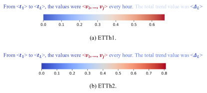
We visualize the last token attention from the last layer of GPT2. First, we segment the words and values in the prompt into nine segments. Then, we visualize the attention of the last segment to the previous eight segments to verify which part of the last token receives the most attention. The results are shown in Figure 7, where we visualize the last token attention on ETTh1 and ETTh2. The last token pays the highest attention to the fifth segment on both datasets, corresponding to the values in our prompt. Therefore, the last token in our designed prompt can save computing costs while maximizing value information for efficient and accurate time series forecasting.

5.5.3. Encoder attention analysis.

(a) Time series encoder attention.

(b) Prompt encoder attention.

Figure 8. Encoder attention visualization.

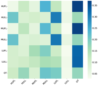
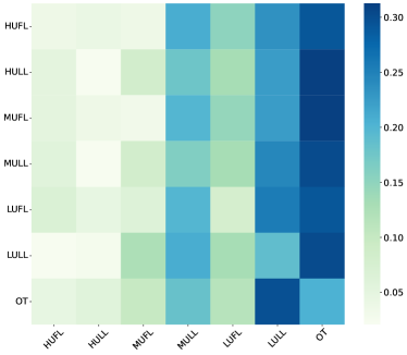
We visualize the variable attention from the time series and prompt encoders, as shown in Figure 8. The time series encoder attention is acquired by a Pre-LN Transformer encoder, while the prompt encoder attention is generated by a frozen LLM. The LLM attention is universal and captures global dependencies between variables, enhancing the model’s ability to understand data relationships. Specifically, in Figure 8 (a), the attention map shows how the Transformer encoder distributes its attention across different variables. This localized attention helps capture the intricate temporal dependencies within the time series data. In Figure 8 (b), The attention map illustrates how the frozen LLM encoder allocates attention. Unlike the time series encoder, the LLM simultaneously focuses on a broader range of variables, indicating its capability to capture global dependencies effectively. Additionally, the prompt encoder attention helps identify which variables are relatively important, offering insights into the key drivers of the data. These visualizations demonstrate that integrating a frozen LLM with a time series encoder enables the model to leverage local and global dependencies, thereby improving its overall forecasting performance.

5.5.4. T-SNE visualization.

(a) Time series embeddings.

(b) Prompt embeddings.

(c) Aligned embeddings.

(d) Forecasted time series embeddings.

Figure 9. T-SNE visualization. (a) Time series embeddings from time series encoder. (b) Prompt embeddings from prompt encoder. (c) Aligned embedding from cross-modality alignment. (d) Forecasted embeddings from projection.

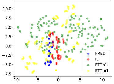
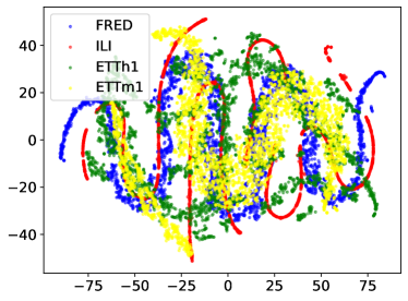
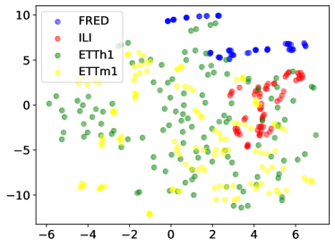
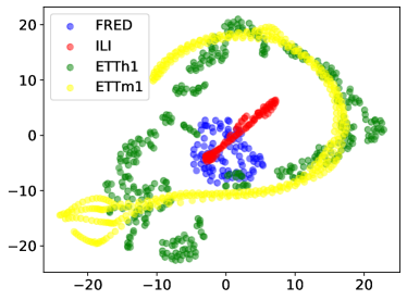
Figure 9 presents a T-SNE visualization of different stages in a multi-modal learning process involving time series and prompt embeddings on ETTh1, ETTm1, ILI, and Fred-MD datasets. In Figure 9 (a), the points are clustered by dataset, indicating that the time series encoder can capture the distinct characteristics of each dataset. In contrast, prompt embeddings in Figure 9 (b) show more complex inter-relations. The alignment in Figure  9 (c) brings similar types of data points (across modalities) closer together, which improves the clustering, indicating effective integration of time series and prompt embeddings. Finally, Figure 9 (d) illustrates that the forecasted time series embeddings form well-separated clusters for each dataset. This suggests that the projection effectively utilizes the aligned embeddings to generate accurate forecasts. Overall, the step-by-step refinement shows how the TimeCMA improves understanding and representation of the data through each stage, culminating in a high-quality output.

6. conclusion

In this paper, we develop TimeCMA, an LLM-empowered framework with cross-modality alignment for multivariate time series forecasting. In our TimeCMA, a dual-modality encoding is implemented in that the time series encoding branch extracts numerical embeddings while the LLM-empowered encoding branch derives high-quality prompt embeddings. Additionally, a cross-modality alignment module is employed to retrieve relevant high-quality and pure time series embedding from the prompt embeddings. Furthermore, TimeCMA shows promise in using the last token embedding of the prompt to reduce the computational cost and enhance the time series forecasting robustly. Sufficient evaluations demonstrate the accuracy and efficiency of TimeCMA compared to existing solutions.

References

- (1)
- Asuncion and Newman (2007) Arthur Asuncion and David Newman. 2007. UCI machine learning repository.
- BehnamGhader et al. (2024) Parishad BehnamGhader, Vaibhav Adlakha, Marius Mosbach, Dzmitry Bahdanau, Nicolas Chapados, and Siva Reddy. 2024. Llm2vec: Large language models are secretly powerful text encoders. arXiv (2024).
- Campos et al. (2021) David Campos, Tung Kieu, Chenjuan Guo, Feiteng Huang, Kai Zheng, Bin Yang, and Christian S. Jensen. 2021. Unsupervised Time Series Outlier Detection with Diversity-Driven Convolutional Ensembles. VLDB 15, 3 (2021), 611–623.
- Campos et al. (2023) David Campos, Miao Zhang, Bin Yang, Tung Kieu, Chenjuan Guo, and Christian S. Jensen. 2023. LightTS: Lightweight Time Series Classification with Adaptive Ensemble Distillation. SIGMOD 1, 2 (2023), 171:1–171:27.
- Cao et al. (2024) Defu Cao, Furong Jia, Sercan O Arik, Tomas Pfister, Yixiang Zheng, Wen Ye, and Yan Liu. 2024. TEMPO: Prompt-based Generative Pre-trained Transformer for Time Series Forecasting. In ICLR.
- Cheng et al. (2023) Yunyao Cheng, Peng Chen, Chenjuan Guo, Kai Zhao, Qingsong Wen, Bin Yang, and Christian S. Jensen. 2023. Weakly Guided Adaptation for Robust Time Series Forecasting. VLDB 17, 4 (2023), 766–779.
- Eichinger et al. (2015) Frank Eichinger, Pavel Efros, Stamatis Karnouskos, and Klemens Böhm. 2015. A time-series compression technique and its application to the smart grid. The VLDB Journal 24 (2015), 193–218.
- Gruver et al. (2023) Nate Gruver, Marc Finzi, Shikai Qiu, and Andrew Gordon Wilson. 2023. Large Language Models Are Zero-Shot Time Series Forecasters. In NeurIPS.
- Hastie et al. (2009) Trevor Hastie, Robert Tibshirani, and Jerome H. Friedman. 2009. The Elements of Statistical Learning: Data Mining, Inference, and Prediction, 2nd Edition.
- Hettige et al. (2024) Kethmi Hirushini Hettige, Jiahao Ji, Shili Xiang, Cheng Long, Gao Cong, and Jingyuan Wang. 2024. AirPhyNet: Harnessing Physics-Guided Neural Networks for Air Quality Prediction. In ICLR.
- Huang et al. (2023) Lei Huang, Jie Qin, Yi Zhou, Fan Zhu, Li Liu, and Ling Shao. 2023. Normalization Techniques in Training DNNs: Methodology, Analysis and Application. IEEE Trans. Pattern Anal. Mach. Intell. 45, 8 (2023), 10173–10196.
- Jin et al. (2024a) Ming Jin, Shiyu Wang, Lintao Ma, Zhixuan Chu, James Y Zhang, Xiaoming Shi, Pin-Yu Chen, Yuxuan Liang, Yuan-Fang Li, Shirui Pan, and Qingsong Wen. 2024a. Time-LLM: Time series forecasting by reprogramming large language models. In ICLR.
- Jin et al. (2024b) Ming Jin, Yifan Zhang, Wei Chen, Kexin Zhang, Yuxuan Liang, Bin Yang, Jindong Wang, Shirui Pan, and Qingsong Wen. 2024b. Position Paper: What Can Large Language Models Tell Us about Time Series Analysis. In ICML.
- Karatzoglidi et al. (2021) Mary Karatzoglidi, Paraskevas Kerasiotis, and Verena Kantere. 2021. Automated energy consumption forecasting with EnForce. VLDB 14, 12 (2021), 2771–2774.
- Kim et al. (2022) Taesung Kim, Jinhee Kim, Yunwon Tae, Cheonbok Park, Jang-Ho Choi, and Jaegul Choo. 2022. Reversible Instance Normalization for Accurate Time-Series Forecasting against Distribution Shift. In ICLR.
- Kitaev et al. (2020) Nikita Kitaev, Lukasz Kaiser, and Anselm Levskaya. 2020. Reformer: The Efficient Transformer. In ICLR.
- Lai et al. (2018) Guokun Lai, Wei-Cheng Chang, Yiming Yang, and Hanxiao Liu. 2018. Modeling Long- and Short-Term Temporal Patterns with Deep Neural Networks. In SIGIR. 95–104.
- Lin et al. (2024) Zhenghao Lin, Zhibin Gou, Yeyun Gong, Xiao Liu, Yelong Shen, Ruochen Xu, Chen Lin, Yujiu Yang, Jian Jiao, Nan Duan, et al. 2024. Rho-1: Not All Tokens Are What You Need. arXiv (2024).
- Liu et al. (2024b) Chenxi Liu, Sun Yang, Qianxiong Xu, Zhishuai Li, Cheng Long, Ziyue Li, and Rui Zhao. 2024b. Spatial-temporal large language model for traffic prediction. In MDM.
- Liu et al. (2024a) Xu Liu, Junfeng Hu, Yuan Li, Shizhe Diao, Yuxuan Liang, Bryan Hooi, and Roger Zimmermann. 2024a. UniTime: A Language-Empowered Unified Model for Cross-Domain Time Series Forecasting. In WWW.
- Liu et al. (2023) Yong Liu, Tengge Hu, Haoran Zhang, Haixu Wu, Shiyu Wang, Lintao Ma, and Mingsheng Long. 2023. iTransformer: Inverted Transformers Are Effective for Time Series Forecasting. In ICLR.
- Liu et al. (2022) Yong Liu, Haixu Wu, Jianmin Wang, and Mingsheng Long. 2022. Non-stationary Transformers: Exploring the Stationarity in Time Series Forecasting. In NeurIPS.
- McCracken and Ng (2016) Michael W McCracken and Serena Ng. 2016. FRED-MD: A monthly database for macroeconomic research. Journal of Business & Economic Statistics 34, 4 (2016), 574–589.
- Nie et al. (2023) Yuqi Nie, Nam H. Nguyen, Phanwadee Sinthong, and Jayant Kalagnanam. 2023. A Time Series is Worth 64 Words: Long-term Forecasting with Transformers. In ICLR.
- Niu et al. (2020) Tong Niu, Jianzhou Wang, Haiyan Lu, Wendong Yang, and Pei Du. 2020. Developing a deep learning framework with two-stage feature selection for multivariate financial time series forecasting. Expert Syst. Appl. 148 (2020), 113237.
- Qiu et al. (2024) Xiangfei Qiu, Jilin Hu, Lekui Zhou, Xingjian Wu, Junyang Du, Buang Zhang, Chenjuan Guo, Aoying Zhou, Christian S. Jensen, Zhenli Sheng, and Bin Yang. 2024. TFB: Towards Comprehensive and Fair Benchmarking of Time Series Forecasting Methods. VLDB (2024).
- Radford et al. (2018) Alec Radford, Karthik Narasimhan, Tim Salimans, Ilya Sutskever, et al. 2018. Improving language understanding by generative pre-training. (2018).
- Radford et al. (2019) Alec Radford, Jeffrey Wu, Rewon Child, David Luan, Dario Amodei, Ilya Sutskever, et al. 2019. Language models are unsupervised multitask learners. OpenAI blog 1, 8 (2019), 9.
- Schmidl et al. (2022) Sebastian Schmidl, Phillip Wenig, and Thorsten Papenbrock. 2022. Anomaly Detection in Time Series: A Comprehensive Evaluation. VLDB 15, 9 (2022), 1779–1797.
- Smith and Demetsky (1997) Brian L Smith and Michael J Demetsky. 1997. Traffic flow forecasting: comparison of modeling approaches. Journal of transportation engineering 123, 4 (1997), 261–266.
- Trindade (2015) Artur Trindade. 2015. Electricity load diagrams 2011–2014. UCI Machine Learning Repository.
- Wu et al. (2023) Haixu Wu, Tengge Hu, Yong Liu, Hang Zhou, Jianmin Wang, and Mingsheng Long. 2023. TimesNet: Temporal 2D-Variation Modeling for General Time Series Analysis. In ICLR.
- Wu et al. (2021a) Haixu Wu, Jiehui Xu, Jianmin Wang, and Mingsheng Long. 2021a. Autoformer: Decomposition Transformers with Auto-Correlation for Long-Term Series Forecasting. In AAAI. 22419–22430.
- Wu et al. (2021b) Xinle Wu, Dalin Zhang, Chenjuan Guo, Chaoyang He, Bin Yang, and Christian S. Jensen. 2021b. AutoCTS: Automated Correlated Time Series Forecasting. VLDB 15, 4 (2021), 971–983.
- Xiong et al. (2020) Ruibin Xiong, Yunchang Yang, Di He, Kai Zheng, Shuxin Zheng, Chen Xing, Huishuai Zhang, Yanyan Lan, Liwei Wang, and Tie-Yan Liu. 2020. On Layer Normalization in the Transformer Architecture. In ICML, Vol. 119. 10524–10533.
- Xue and Salim (2023) Hao Xue and Flora D. Salim. 2023. PromptCast: A New Prompt-Based Learning Paradigm for Time Series Forecasting. TKDE (2023), 1–14.
- Xue et al. (2022) Hao Xue, Bhanu Prakash Voutharoja, and Flora D. Salim. 2022. Leveraging language foundation models for human mobility forecasting. In SIGSPATIAL. 90:1–90:9.
- Zeng et al. (2023) Ailing Zeng, Muxi Chen, Lei Zhang, and Qiang Xu. 2023. Are Transformers Effective for Time Series Forecasting?. In AAAI.
- Zhang et al. (2021) Shanghang Zhang, Jieqi Peng, Shuai Zhang, Jianxin Li, Hui Xiong, and Wancai Zhang. 2021. Informer: Beyond Efficient Transformer for Long Sequence Time-Series Forecasting. In AAAI. 11106–11115.
- Zhang and Yan (2023) Yunhao Zhang and Junchi Yan. 2023. Crossformer: Transformer Utilizing Cross-Dimension Dependency for Multivariate Time Series Forecasting. In ICLR.
- Zhao et al. (2023) Kai Zhao, Chenjuan Guo, Yunyao Cheng, Peng Han, Miao Zhang, and Bin Yang. 2023. Multiple Time Series Forecasting with Dynamic Graph Modeling. VLDB 17, 4 (2023), 753–765.
- Zhou et al. (2022) Tian Zhou, Ziqing Ma, Qingsong Wen, Xue Wang, Liang Sun, and Rong Jin. 2022. FEDformer: Frequency Enhanced Decomposed Transformer for Long-term Series Forecasting. In ICML, Vol. 162. 27268–27286.
- Zhou et al. (2023) Tian Zhou, Peisong Niu, Xue Wang, Liang Sun, and Rong Jin. 2023. One Fits All: Power General Time Series Analysis by Pretrained LM. In NeurIPS.