Equivariant Amortized Inference of Poses for Cryo-EM
Abstract
Cryo-EM is a vital technique for determining 3D structure of biological molecules such as proteins and viruses. The cryo-EM reconstruction problem is challenging due to the high noise levels, the missing poses of particles, and the computational demands of processing large datasets. A promising solution to these challenges lies in the use of amortized inference methods, which have shown particular efficacy in pose estimation for large datasets. However, these methods also encounter convergence issues, often necessitating sophisticated initialization strategies or engineered solutions for effective convergence. Building upon the existing cryoAI pipeline, which employs a symmetric loss function to address convergence problems, this work explores the emergence and persistence of these issues within the pipeline. Additionally, we explore the impact of equivariant amortized inference on enhancing convergence. Our investigations reveal that, when applied to simulated data, a pipeline incorporating an equivariant encoder not only converges faster and more frequently than the standard approach but also demonstrates superior performance in terms of pose estimation accuracy and the resolution of the reconstructed volume. Notably, -equivariant encoders make the symmetric loss superfluous and, therefore, allow for a more efficient reconstruction pipeline.
1 Introduction
Cryo-electron microscopy (cryo-EM) has emerged as an crucial technique in molecular biology and chemistry, enabling the determination of macro-molecular structures such as proteins. In cryo-EM, particle samples are frozen in a thin layer of vitreous ice and exposed to an electron beam. The interaction between electrons and the sample’s electrostatic potential scatters electrons in patterns that reflect the molecular structure. This results in multiple noisy two-dimensional projections of the particles in random orientations, which are then used to reconstruct the molecular structure.
The reconstruction process presents significant challenges, including the estimation of unknown poses and the high noise levels Singer & Shkolnisky (2011); Singer & Sigworth (2020). Traditional methods employ iterative approaches that, in each step, require extensive searches over the space of poses for each datapoint and a refinement of the molecular structure estimate (e.g. maximum-likelihood expectation-maximization (ML-EM) implemented by SOTA softwares like RELION Scheres (2012) and cryoSPARC Punjani et al. (2017)); however, this per-image search doesn’t scale well with the increasing datasets sizes due its computational demand Levy et al. (2022a).
Recently, deep learning approaches have shown promise in addressing these challenges, giving rise to a new category of reconstruction methods based on amortized inference Giri et al. (2023). These methods learn a parametrized function, typically within a framework employing (variational) autoencoder architectures, to predict particle poses from images, shifting the computational burden to the learning phase. Although this reduces the need for per-image pose estimation, these solutions often face convergence issues, requiring careful engineering to achieve satisfactory performance.
Contributions
We introduce equivariant amortized inference of poses for cryo-EM. This method uses the property that images that differ by some in-plane rotation or mirroring have associated poses that undergo a similar transformation. In the amortized inference framework, we can exploit this prior knowledge of the geometry of the problem by making the parameterized function equivariant with respect to rotations and/or reflections. Using an equivariant function has the following benefits:
-
•
faster generalization faster reconstruction: once it learns to predict the pose of an image correctly, it immediately generalizes to rotations and reflection of that particular image. This typically also leads to faster convergence and, thus, to faster reconstruction here.
-
•
geometrical consistency = reduced convergence issues: it is forced from the start to represent subsets of datapoints according to the correct underlying geometric structure, potentially reducing or preventing the convergence issues discussed earlier.
2 Image formation model
We can model the electrostatic potential of a molecule as a 3D density, . Each molecule, frozen in ice, assumes a random orientations represented by a rotation . The image is formed by electrons that are scattered by interacting with this potential, hitting a detector. This is modeled as a projection:
| (1) |
Before the electrons hit the detector, they interact with the lens system of the microscope, represented by a convolution with a Point Spread Function (PSF) kernel . Additionally, we account for small translations by convolving with the translation kernel and add a Gaussian noise variable to model various noise sources. The resulting image formation model is:
| (2) |
We assume square integrable functions, i.e. and . The image formation model is usually formulated and implemented in Fourier space, which we describe in Apx. A.
3 Related work
Amortized inference of poses for cryo-EM
Recently, deep learning based methods have been applied to the cryo-EM reconstruction problem (Donnat et al., 2022; Giri et al., 2023). With this, a new approach has emerged: amortized inference over poses. Such methods learn a parametrized function that estimates a pose given an image, as opposed to estimating the pose for each image individually. Typically, (variational) autoencoder architectures are employed in this setting. For example, Rosenbaum et al. (2021) use a variational autoencoder architecture in a heterogeneous setting in which the encoder predicts both poses and conformations. CryoVAEGAN (Miolane et al., 2020) is a pipeline in which an encoder estimates rotations as well as parameters of the contrast transfer function (CTF). In the spatialVAE pipeline the encoder estimates translations and in-plane rotations Bepler et al. (2019). CryoPoseNet (Nashed et al., 2021), cryoAI (Levy et al., 2022a) and cryoFIRE (Levy et al., 2022b) demonstrate the efficacy of an autoencoder (AE) architecture in which the encoder learns to estimate poses. While promising, amortized inference methods may suffer from convergence issues. For example, in (Rosenbaum et al., 2021), a strong prior on the backbone of the molecule is needed for the pipeline to converge. CryoPoseNet tends to get stuck in local minima while cryoAI and cryoFIRE limit this issue by using an additional symmetric loss.
Homoemorphic Encoders and Equivariance
Falorsi et al. (2018) introduced homeomorphic encoders to describe a setting where the input data has a geometric structure associated with a symmetry group and the goal for the encoder is to learn a homeomorphic geometric representation of the data in the latent space. This is analogous the amortized inference of poses in cryo-EM, as each image is identified by an element of . Esmaeili et al. (2023) show that these models are prone to optimization challenges due to topological defects at initialization that cannot be resolved continuously, partially explaining the convergence issues observed in previous works employing amortized inference of poses. One can incorporate geometric inductive bias into neural networks via equivariance. For example, convolutional neural networks (CNNs) are translation-equivariant. This idea is generalized via group convolution (GCNNs) (Cohen & Welling, 2016a) and Steerable CNNs (Cohen & Welling, 2016b) to achieve equivariance with respect to more general symmetry groups. Cryo-EM images possess a number of symmetries (Cesa et al., 2022a) which can be exploited via an equivariant design. Previously, Nasiri & Bepler (2022); Cesa et al. (2023); Granberry et al. (2023) leveraged some of these planar symmetries. To the best of our knowledge, this is the first work to successfully leverage these symmetries in an end-to-end cryo-EM reconstruction pipeline.
4 Method
4.1 Equivariant amortized inference of poses
We can think of a 3D rotation as an element , where and are the columns of the matrix associated to the rotation. The vectors and form an orthonormal basis of . The operator defined in Eq. 1 first rotates the volume and then performs a
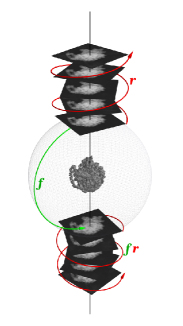
projection along the -axis. Rotating the volume by can be seen as transforming with the transformation that would align and with the standard basis vectors of . Therefore, alternatively, we can see the axis as the ‘direction’ along which the projection is performed. We shall call the axis the viewing direction. Note that two images that are generated by projecting along the same viewing direction can only differ by an in-plane rotation , whereas if they differ by a rotation and a reflection , they are obtained by projecting along opposite viewing directions and , see Fig. 1. In fact, given an element
| (3) |
with if two images and are related such that111 The left action of on an image yields a new image given by . , then we know that their associated poses are related by the following identity:
| (4) |
where is a three-dimensional representation of O; see Apx. D. Poses typically include also planar translations in , which follow an analogous equivariance rule; see Apx. E.1 for more details. In Sec. 4.3, we will exploit this knowledge in the amortized inference framework by restricting the parameterized function mapping images to their associated poses to be equivariant to a subgroup .
4.2 Pipeline overview
We build on the work by Levy et al. (2022a), adapting their autoencoder pipeline by incorporating an equivariant encoder. Given an input image , the encoder predicts a pose existing of a translation and a rotation . The decoder maintains an estimate of the reconstructed volume via an implicit neural representation , which models the Fourier transform of . The decoder simulates the image formation model in Fourier space by leveraging the Fourier Slice Theorem as in Apx. A. : it rotates a slice of three-dimensional coordinates by the rotation and, then, feeds them into . The result is translated by , convoluted with the contrast transfer function; see Apx. B for more details about the decoder. Finally, the output is compared to the input via a mean-squared error loss ( loss).
4.3 Equivariant encoder
We replicate the architecture of the original encoder of cryoAI (see Apx. B of Levy et al. (2022a)) using the escnn Python library Cesa et al. (2022b) to incorporate equivariance to a subgroup ; see Apx. E for more details. We can interpret the encoder as two separate functions: that outputs a rotation, and that outputs a translation. Equivariance ensures that, for any element and image :
| (5) |
In particular, we experimented with equivariance to the and subgroups of . contains the rotations by , while contains these rotations, and their combinations with a reflection. Note that these groups model the exact rotational symmetries of a pixel grid.
4.4 Symmetric loss function
The original pipeline is optimized using a symmetric loss function to reduce convergence issues Levy et al. (2022a). This loss function augments a batch with a duplicate of each image rotated by . For each image and its rotated duplicate, the model is only supervised on the one it reconstructs best. Formally, the symmetric loss is defined as follows:
| (6) |
where is the whole cryoAI pipeline, interpreted as a function and is the left action1 of the rotation by . In the equivariant pipeline, the loss function in Eq. 6 becomes trivial, as both and include the rotation by , and thus . When we use , which includes rotations but no reflections, we adapt the symmetric loss above by replacing by , where is the reflection in Eq. 3. If is used, we refer to the loss as ‘mirror loss’ .
5 Experiments
Simulated datasets with varying noise levels were generated as in Levy et al. (2022a) from the following Protein Data Bank structures: plasmodium falciparum 80S ribosome (PDB: 3J79 and 3J7A) Wong et al. (2014) (80S), and the pre-catalytic spliceosome (PDB: 5NRL) Plaschka et al. (2017) (spliceosome). See Apx. C for more details.
5.1 Convergence of original pipeline
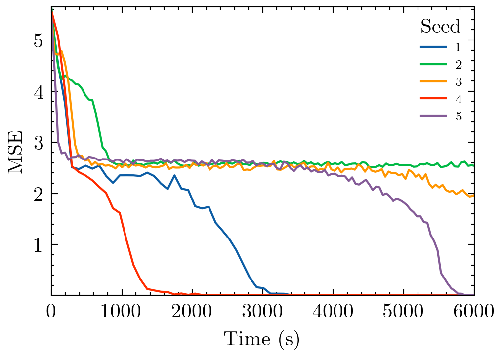
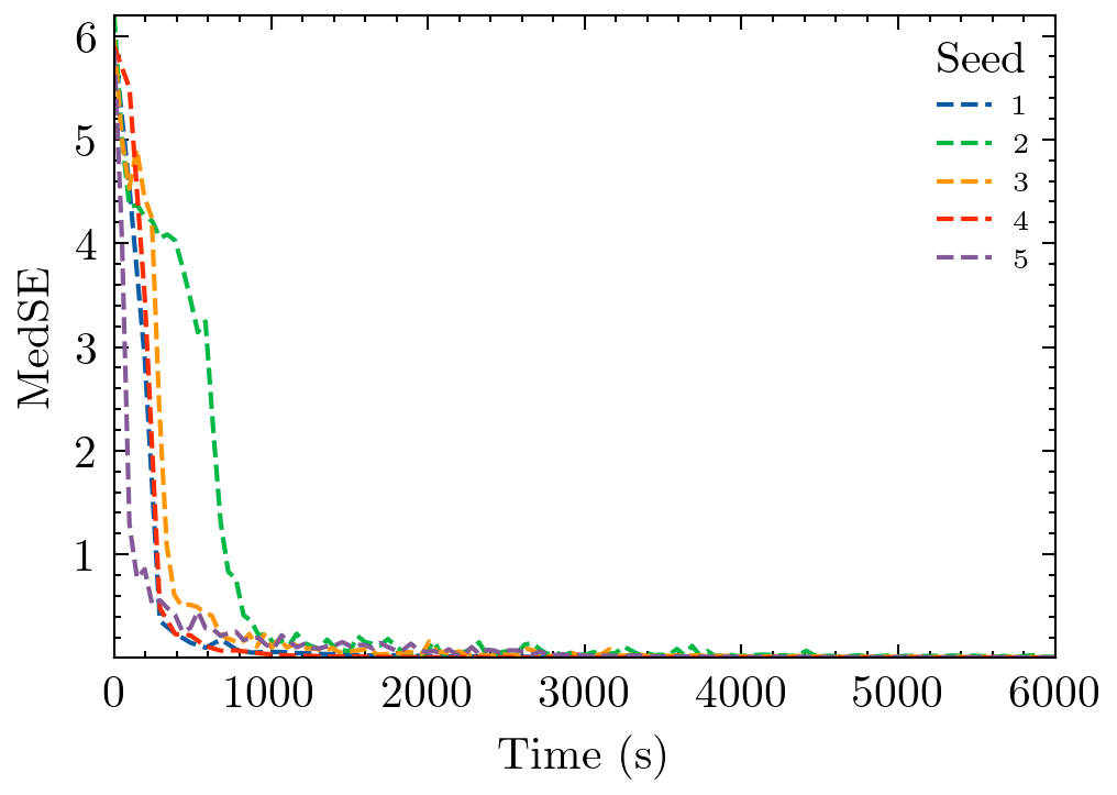
To examine the convergence progress of the original pipeline, cryoAI was trained with a non-equivariant encoder and across datasets for two structures - each with a noiseless and an version - using different seeds for 6000 seconds. Fig. 2 illustrates the trends of Mean Squared Error (MSE) and Median Squared Error (MedSE) for runs using a noiseless spliceosome dataset. The observed pattern shows an initial decline in both MedSE and MSE, with MedSE approaching zero fast and MSE plateauing, then sharply decreasing. This behavior, further analyzed in Apx. G, correlates with transient spurious planar symmetries in volume reconstructions, which resolve as MSE improves. While reduces the duration of such states, they still occur.
5.2 Impact of equivariance on convergence of pipeline
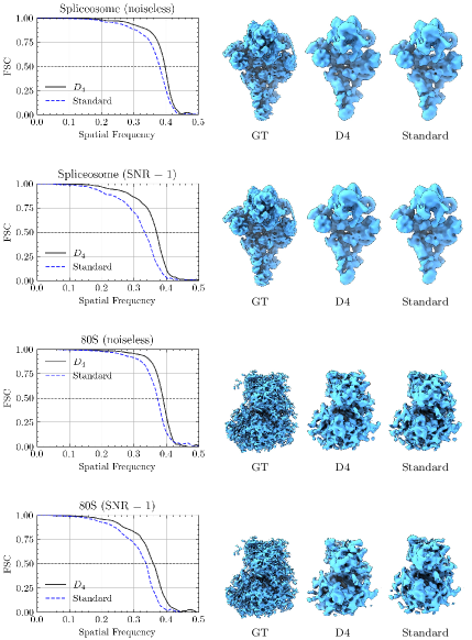
We evaluated - and -equivariant encoders against a standard model using or an loss across four simulated datasets (each for two structures, with and without noise), with seeds per dataset and a 6000-second training limit. Performance metrics including MSE, convergence rates, and volume resolution are summarized in Tab. 1, with metric definitions in Apx. F. Convergence is defined as MSE 0.1 based on experiments with the standard pipeline that showed that the volume escapes symmetric states after the MSE has decreased sufficiently. Our findings reveal that equivariance with loss rarely converges, but it significantly enhances convergence speed and accuracy when paired with . -equivariant encoders reliably converge without , outperforming all other models in speed of convergence and metric performance, as highlighted by the superior resolution and pose estimation accuracy. Moreover, we compare both the Fourier Shell Correlation (FSC) curves and the 3D reconstructions of some of the models in Fig. 3. The -equivariant models consistently yield higher FSC curves, indicating improved reconstruction quality. However, we note that the improved reconstruction quality might still not be enough to provide additional biological insights. Since we are not sufficiently expert to judge this aspect, we leave it for future exploration but emphasize the computational benefits of our method with respect to the standard cryoAI pipeline, particularly in terms of faster reconstruction.
| Dataset | Model | MSE | MedSE |
|
|
|
|
||||||||||
|---|---|---|---|---|---|---|---|---|---|---|---|---|---|---|---|---|---|
| Spliceosome noiseless | Standard () | 0.0040 0.0002 | 0.0030 0.0001 | 2818 286 | 5800 589 | 11.26 0.11 | 62.5 | ||||||||||
| (L2) | 2.5893 0.0322 | 0.0166 0.0090 | - | - | 12.18 0.13 | 0 | |||||||||||
| () | 0.0008 0.0001 | 0.0005 0.0000 | 1457 1001 | 1967 1347 | 11.11 0.19 | 100 | |||||||||||
| (L2) | 0.0004 0.0000 | 0.0003 0.0000 | 1239 782 | 2800 1766 | 10.88 0.18 | 87.5 | |||||||||||
| 80S noiseless | Standard () | 0.0041 0.0001 | 0.0030 0.0001 | 2564 394 | 5300 804 | 10.20 0.10 | 100 | ||||||||||
| (L2) | 0.8160 1.1520 | 0.0020 0.0016 | - | - | 10.35 0.28 | 25 | |||||||||||
| () | 0.0010 0.0000 | 0.0006 0.0000 | 791 195 | 1067 262 | 10.05 0.00 | 100 | |||||||||||
| (L2) | 0.0005 0.0001 | 0.0004 0.0000 | 774 143 | 1767 330 | 9.72 0.09 | 87.5 | |||||||||||
| Spliceosome SNR 1 | Standard () | 0.3232 0.3384 | 0.0077 0.0031 | - | - | 12.72 0.97 | 12.5 | ||||||||||
| (L2) | 2.6525 0.0104 | 0.0308 0.0273 | - | - | 13.06 0.15 | 0 | |||||||||||
| () | 0.0014 0.0001 | 0.0010 0.0001 | 1181 312 | 1600 432 | 11.33 0.00 | 87.5 | |||||||||||
| (L2) | 0.0010 0.0000 | 0.0007 0.0000 | 1624 426 | 3333 998 | 11.03 0.10 | 50 | |||||||||||
| 80S SNR 1 | Standard () | 0.0102 0.0003 | 0.0070 0.0009 | 3093 418 | 6400 909 | 11.22 0.00 | 75 | ||||||||||
| (L2) | 0.0055 0.0014 | 0.0037 0.0009 | 4080 999 | 10100 2491 | 10.97 0.20 | 37.5 | |||||||||||
| () | 0.0038 0.0002 | 0.0027 0.0001 | 1386 808 | 1867 1087 | 10.97 0.00 | 100 | |||||||||||
| (L2) | 0.0032 0.0001 | 0.0023 0.0000 | 1071 135 | 2433 309 | 10.65 0.22 | 100 |
Higher noise levels
To investigate if the convergence benefits of equivariance are maintained under higher noise conditions, we conducted an experiment focusing on the standard model and the -equivariant model. These models were trained on datasets generated using the 80S ribosome structure at various noise levels; see Apx. C. Each model is trained for 6 hours. We recorded the metrics for the best run out of for each model and dataset. The results in Tab. 2 show that the benefits of equivariance hold at higher noise levels. The equivariant encoder outperforms the standard encoder on all metrics for each noise level, except the highest (), although it should be noted that all seeds of both models didn’t converge at that noise level.
| SNR | Model | MSE | MedSE |
|
|
||
|---|---|---|---|---|---|---|---|
| 0.75 | (L2) | 0.0012 | 0.0009 | 1238.04 | 9.46 | ||
| Standard () | 0.0027 | 0.0021 | 3065.58 | 9.65 | |||
| 0.625 | (L2) | 0.0013 | 0.0011 | 1136.72 | 9.56 | ||
| Standard () | 0.0036 | 0.0025 | 2722.84 | 9.85 | |||
| 0.5 | (L2) | 0.0021 | 0.0014 | 1850.60 | 9.75 | ||
| Standard () | 0.0057 | 0.0039 | 3885.72 | 10.72 | |||
| 0.375 | (L2) | 0.0057 | 0.0033 | 6263.10 | 10.97 | ||
| Standard () | 0.0780 | 0.0096 | 12741.46 | 12.37 | |||
| 0.25 | (L2) | 1.4671 | 0.1627 | - | 22.98 | ||
| Standard () | 0.7455 | 0.0546 | - | 16.09 |
6 Final Discussions
Our experiments demonstrate the benefits of incorporating geometric priors in the Cryo-EM amortized inference framework. Indeed, equivariant models consistently show drastic improvements in convergence speed, convergence ratio and final resolution. In particular, -equivariance makes the expensive symmetric loss superfluous. These results indicate that apart from the symmetric loss, equivariant amortized inference can be a viable alternative solution to the convergence issues associated with symmetric reconstructions. Still, some runs with equivariant encoder did not convergence; in this context, Esmaeili et al. (2023) suggested that, while inductive biases like equivariance can guide models towards learning homeomorphic representations, they might also complicate the training process in practice. Inspired by their solution, we find encoders modeling a multimodal distribution, as opposed to our single-pose encoders, to be a promising direction of research.
References
- Bepler et al. (2019) Tristan Bepler, Ellen Zhong, Kotaro Kelley, Edward Brignole, and Bonnie Berger. Explicitly disentangling image content from translation and rotation with spatial-vae. Advances in Neural Information Processing Systems, 32, 2019.
- Cesa et al. (2022a) Gabriele Cesa, Arash Behboodi, Taco S Cohen, and Max Welling. On the symmetries of the synchronization problem in cryo-em: Multi-frequency vector diffusion maps on the projective plane. Advances in Neural Information Processing Systems, 35:5446–5458, 2022a.
- Cesa et al. (2022b) Gabriele Cesa, Leon Lang, and Maurice Weiler. A program to build E(N)-equivariant steerable CNNs. In International Conference on Learning Representations, 2022b. URL https://openreview.net/forum?id=WE4qe9xlnQw.
- Cesa et al. (2023) Gabriele Cesa, Kumar Pratik, and Arash Behboodi. Equivariant self-supervised deep pose estimation for Cryo EM. In Proceedings of 2nd Annual Workshop on Topology, Algebra, and Geometry in Machine Learning (TAG-ML), Proceedings of Machine Learning Research. PMLR, 28 Jul 2023.
- Cohen & Welling (2016a) Taco Cohen and Max Welling. Group equivariant convolutional networks. In International conference on machine learning, pp. 2990–2999. PMLR, 2016a.
- Cohen & Welling (2016b) Taco S Cohen and Max Welling. Steerable CNNs. arXiv preprint arXiv:1612.08498, 2016b.
- Donnat et al. (2022) Claire Donnat, Axel Levy, Frederic Poitevin, Ellen D Zhong, and Nina Miolane. Deep generative modeling for volume reconstruction in cryo-electron microscopy. Journal of Structural Biology, pp. 107920, 2022.
- Esmaeili et al. (2023) Babak Esmaeili, Robin Walters, Heiko Zimmermann, and Jan-Willem van de Meent. Topological obstructions and how to avoid them. arXiv preprint arXiv:2312.07529, 2023.
- Falorsi et al. (2018) Luca Falorsi, Pim De Haan, Tim R Davidson, Nicola De Cao, Maurice Weiler, Patrick Forré, and Taco S Cohen. Explorations in homeomorphic variational auto-encoding. arXiv preprint arXiv:1807.04689, 2018.
- Giri et al. (2023) Nabin Giri, Raj S Roy, and Jianlin Cheng. Deep learning for reconstructing protein structures from cryo-em density maps: Recent advances and future directions. Current Opinion in Structural Biology, 79:102536, 2023.
- Granberry et al. (2023) Darnell Granberry, Simons Machine Learning Center, Alireza Nasiri, Jiayi Shou, Alex J Noble, and Tristan Bepler. So (3)-equivariant representation learning in 2d images. In NeurIPS 2023 Workshop on Symmetry and Geometry in Neural Representations, 2023.
- Levinson et al. (2020) Jake Levinson, Carlos Esteves, Kefan Chen, Noah Snavely, Angjoo Kanazawa, Afshin Rostamizadeh, and Ameesh Makadia. An analysis of svd for deep rotation estimation. Advances in Neural Information Processing Systems, 33:22554–22565, 2020.
- Levy et al. (2022a) Axel Levy, Frédéric Poitevin, Julien Martel, Youssef Nashed, Ariana Peck, Nina Miolane, Daniel Ratner, Mike Dunne, and Gordon Wetzstein. Cryoai: Amortized inference of poses for ab initio reconstruction of 3d molecular volumes from real cryo-em images. In European Conference on Computer Vision, pp. 540–557. Springer, 2022a.
- Levy et al. (2022b) Axel Levy, Gordon Wetzstein, Julien NP Martel, Frederic Poitevin, and Ellen Zhong. Amortized inference for heterogeneous reconstruction in cryo-em. Advances in Neural Information Processing Systems, 35:13038–13049, 2022b.
- Meng et al. (2023) Elaine C Meng, Thomas D Goddard, Eric F Pettersen, Greg S Couch, Zach J Pearson, John H Morris, and Thomas E Ferrin. Ucsf chimerax: Tools for structure building and analysis. Protein Science, 32(11):e4792, 2023.
- Miolane et al. (2020) Nina Miolane, Frédéric Poitevin, Yee-Ting Li, and Susan Holmes. Estimation of orientation and camera parameters from cryo-electron microscopy images with variational autoencoders and generative adversarial networks. In Proceedings of the IEEE/CVF Conference on Computer Vision and Pattern Recognition Workshops, pp. 970–971, 2020.
- Nashed et al. (2021) Youssef SG Nashed, Frédéric Poitevin, Harshit Gupta, Geoffrey Woollard, Michael Kagan, Chun Hong Yoon, and Daniel Ratner. Cryoposenet: end-to-end simultaneous learning of single-particle orientation and 3d map reconstruction from cryo-electron microscopy data. In Proceedings of the IEEE/CVF International Conference on Computer Vision, pp. 4066–4076, 2021.
- Nasiri & Bepler (2022) Alireza Nasiri and Tristan Bepler. Unsupervised object representation learning using translation and rotation group equivariant vae. Advances in Neural Information Processing Systems, 35:15255–15267, 2022.
- Plaschka et al. (2017) Clemens Plaschka, Pei-Chun Lin, and Kiyoshi Nagai. Structure of a pre-catalytic spliceosome. Nature, 546(7660):617–621, 2017.
- Punjani et al. (2017) Ali Punjani, John L Rubinstein, David J Fleet, and Marcus A Brubaker. cryosparc: algorithms for rapid unsupervised cryo-em structure determination. Nature methods, 14(3):290–296, 2017.
- Rosenbaum et al. (2021) Dan Rosenbaum, Marta Garnelo, Michal Zielinski, Charlie Beattie, Ellen Clancy, Andrea Huber, Pushmeet Kohli, Andrew W Senior, John Jumper, Carl Doersch, et al. Inferring a continuous distribution of atom coordinates from cryo-em images using vaes. arXiv preprint arXiv:2106.14108, 2021.
- Scheres (2012) Sjors HW Scheres. Relion: implementation of a bayesian approach to cryo-em structure determination. Journal of structural biology, 180(3):519–530, 2012.
- Singer & Shkolnisky (2011) Amit Singer and Yoel Shkolnisky. Three-dimensional structure determination from common lines in cryo-em by eigenvectors and semidefinite programming. SIAM journal on imaging sciences, 4(2):543–572, 2011.
- Singer & Sigworth (2020) Amit Singer and Fred J Sigworth. Computational methods for single-particle electron cryomicroscopy. Annual review of biomedical data science, 3:163–190, 2020.
- Sitzmann et al. (2020) Vincent Sitzmann, Julien Martel, Alexander Bergman, David Lindell, and Gordon Wetzstein. Implicit neural representations with periodic activation functions. Advances in neural information processing systems, 33:7462–7473, 2020.
- Weiler & Cesa (2019) Maurice Weiler and Gabriele Cesa. General E(2)-equivariant steerable CNNs. Advances in neural information processing systems, 32, 2019.
- Wong et al. (2014) Wilson Wong, Xiao-chen Bai, Alan Brown, Israel S Fernandez, Eric Hanssen, Melanie Condron, Yan Hong Tan, Jake Baum, and Sjors HW Scheres. Cryo-em structure of the plasmodium falciparum 80s ribosome bound to the anti-protozoan drug emetine. Elife, 3:e03080, 2014.
Appendix A Image formation model in Fourier space
Implementing the image formation model in reconstruction algorithms can become computationally expensive due to the rotation of the volume and the integral in equation 1. Formulating the image formation in Fourier space allows for the application of the Fourier Slice Theorem, which makes rotating and integrating the volume redundant.
The theorem states that evaluating a volume on a plane (‘a slice of coordinates’) in Fourier space gives the Fourier transform of a projection of that volume along an axis perpendicular to that plane. In mathematical terms, this means that
| (7) |
where and are the two- and three dimensional Fourier transforms, and is an operator that performs the operation of evaluating a volume on a plane, and is defined such that
| (8) |
Using the Fourier Slice Theorem, we can formulate the entire image formation model in Fourier space as follows:
| (9) |
Here is the Fourier transform of the kernel, called the Contrast Transfer Function (CTF), is the translation operator performing in Fourier space (which corresponds to a phase shift) and is i.i.d. complex Gaussian noise at each frequency. The symbol stands for element-wise multiplication that replaces convolution in the real formulation, which follows from the Convolution Theorem.
Appendix B Decoder architecture
The decoder takes the rotation and the translation outputted by the encoder as an input. An array of three-dimensional coordinates is generated that represent the Fourier frequencies corresponding to a grid of coordinates on the plane. Each coordinate in this slice is then rotated by and fed into a neural network . The network , called FourierNet, represents the Fourier transform of the electrostatic potential of the molecule that we wish to reconstruct.
FourierNet consists of two SIREN models that take a coordinate and output a vector in . SIREN (Sinusoidal Representation) networks are fully connected feed-forward neural networks that utilize sinusoidal activation functions. SIREN networks have been shown to be successful in representing complex signals defined on real space. (Sitzmann et al. (2020)) The Fourier transform of an electrostatic of a molecule is known to vary in magnitude over several orders of magnitude. (Levy et al. (2022a)) To allow FourierNet to represent a function that varies several orders of magnitude in value, one of the two SIRENs has the property that the exponential function is applied element-wise on its output.
To ensure that the network actually represents a Fourier transform, the following property is enforced
| (10) |
simply by following this as a definition. The two output vectors of the networks are multiplied element-wise and the result is interpreted as an element of via the mapping
Since the input to FourierNet was a slice of three-dimensional coordinates, the output represents a slice of a Fourier transform as defined in Eq. 7. The final output of the decoder is obtained as follows:
| (11) |
where is the CTF, and is the translation operator performing the translation predicted by the encoder in Fourier space. The CTF is a function of parameters that can be estimated from the dataset and are assumed to be known. For more details about the pipeline architecture, see Levy et al. (2022a).
Appendix C Data
The data was synthesized with structures from the Protein Data Bank. The two structures that were used were the plasmodium falciparum 80S ribosome structure (PDB: 3J79 and 3J7A) Wong et al. (2014) and the pre-catalytic spliceosome structure (PDB: 5NRL) Plaschka et al. (2017).
The plasmodium falciparum 80S ribosome volume.
[.45]![[Uncaptioned image]](/html/2406.01630/assets/Figures/80s.png) [.4]
[.4]![[Uncaptioned image]](/html/2406.01630/assets/Figures/spliceosome.png)
The pre-catalytic spliceosome volume.
The datasets were generated by simulating the image formation model described in Sec. 2 using ground-truth volume represented as a three-dimensional voxel grid, as in Levy et al. (2022a). The volume data for the ground truth volumes was generated in ChimeraX Meng et al. (2023) as described in Apx. A.1 of Levy et al. (2022a). See Fig. 4(a) for a visualization of the volumes.
Each dataset contains images of dimension . The simulator uses poses randomly sampled from a uniform distribution over SO, and translations sampled from a Gaussian distribution with mean zero and a standard deviation of Å.
For both the pre-catalytic spliceosome and the plasmodium falciparum 80S ribosome structures, one noisless dataset was generated, and one with signal-to-noise ratio (SNR) equal to . For the plasmodium falciparum 80S ribosome structure, additional datasets were generated with SNR and , in Fig. 5 we show examples of images from each of the datasets generated with the plasmodium falciparum 80S ribosome.
Noiseless
[.14]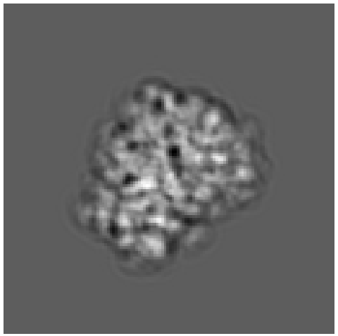 [.14]
[.14]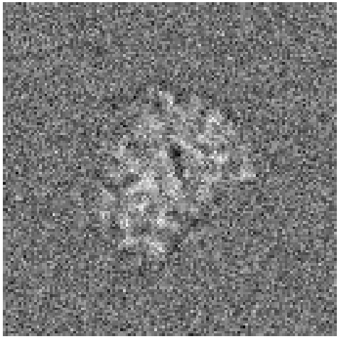 [.14]
[.14]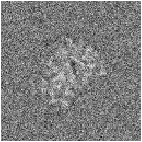 [.14]
[.14]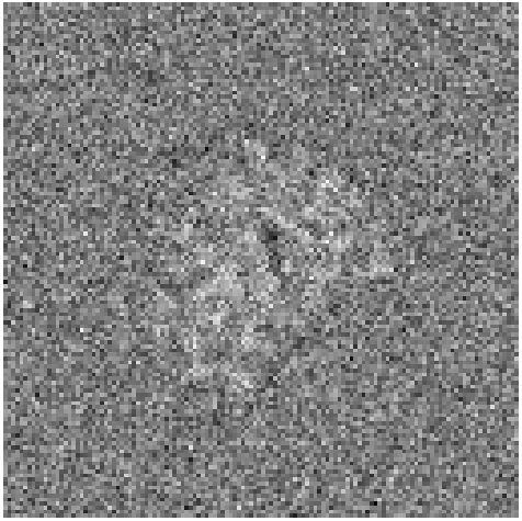 [.14]
[.14]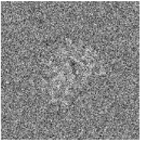 [.14]
[.14]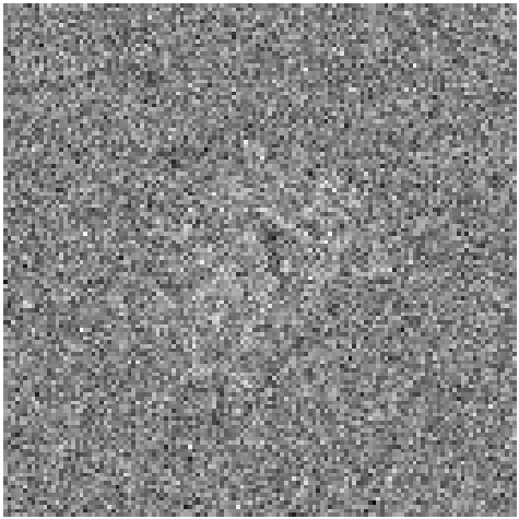 [.14]
[.14]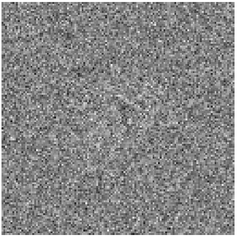
SNR
SNR
SNR
SNR
SNR
SNR
Appendix D Background on Group and Group Representation Theory
Group theory, and specifically group representation theory, are important building blocks in the theory about equivariant neural networks, such as steerable networks that are applied in this work. In this Section we provide some important definitions and preliminaries that are useful for understanding the method presented in this work.
Groups can be useful to describe the structure of sets of geometrical transformations, such as rotations and translations. We start by giving the definition of a group.
Another important definition in group theory is that of a group homomorphism. Intuitively, group homomorphisms are functions between groups that preserve algebraic structure shared by these groups.
It can be useful to ‘combine’ several groups into one. In this way we can represent different types of transformations (e.g. translation and rotation) as elements of a single group. One way to do this is via semi-direct products.
As mentioned, some groups describe the structure of sets of geometrical transformations, such as rotations and translations. Such groups have actions on other spaces. Group representations are one way to describe the actions of certain groups (linear transformations) on vector spaces. To define group representations, we first give the definition of the general linear group:
Since in deep learning we are often working with real-valued vectors, when we refer to the general linear group, we are usually talking about GL(). This is the group of all invertible matrices.
Using the definition of the general linear group, we can define group representations.
Some examples of representations follow below.
By looking at a representation of the circle group that we defined before, we see that the circle group is actually also a group that describes a specific type of transformation on : rotations.
We can combine multiple representations together into a single representation via the direct sum. This concept is important in the theory of steerable CNNs.
An important representation in the theory of steerable CNNs is the regular representation.
We finish this section with some important groups that we regularly refer to in this work. The first group, SO, contains all three-dimensional rotation matrices.
Another important group, , contains two-dimensional rotations and reflections.
Finally, the groups and are both subgroups of O.
Appendix E Equivariant encoder architecture
A high-level overview of the equivariant encoder is shown in Figure 6. As mentioned in Section 4.2, the architecture was kept as similar as possible to the standard pipeline in Levy et al. (2022a). The encoders were implemented as steerable CNNs Cohen & Welling (2016b) with the escnn Python library Weiler & Cesa (2019); Cesa et al. (2022b)
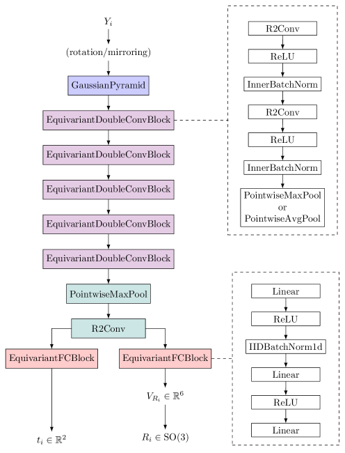
If a symmetric- or mirror loss function (see Section 4.4) is used, the input is fed into a sym layer. This layer performs the operation of duplicating the batch of images and then rotating it by or mirroring it with respect to the -axis (depending on the type of loss). The transformed images are concatenated batch-wise. If an L loss function is used, this process is skipped. The batch then goes into a GaussianPyramid layer with five Gaussian filters of size with cutoff frequencies that are geometrically distributed between 0.1 and 10 pix-1 (as in Levy et al. (2022a)), that filter each image.
The filtered images are fed into five consecutive EquivariantDoubleConvBlock networks. Each EquivariantDoubleConvBlock layer is made up of two convolutional layers with steerable kernels (R2Conv) and a PointwiseMaxPool layer. Each of the R2Conv layers is followed by a pointwise ReLU activation function and an InnerBatchNorm layer.
After passing through each of the EquivariantDoubleConvBlock blocks, the batch passes through a PointwiseMaxPool layer and a single R2Conv layer with a kernel of size . This results in an output with a width and height of , with overal shape This output is fed into two separate equivariant fully connected networks (EquivariantFCBlock). The first EquivariantFCBlock outputs a vector , which is directly interpreted as a translation. The second EquivariantFCBlock outputs a vector , which is then mapped to and interpreted as a rotation matrix as explained in Apx. E.1.
E.1 Technical details
In this section we present some technical details related to the implementation of the encoder. We start with some very brief theory.
Recall that in regular CNNs, layers are convolution operators that, when applied to an input, yield a feature map. A key difference between steerable CNNs and regular CNNs is that in the former, feature maps are replaced by steerable feature fields:
Layers in steerable CNNs are equivariant, meaning that if a feature field is transformed by a group element according to its transformation law and then passes through a layer, we want this to give the same output as the feature field first passing through that layer and then transforming the generated feature field by the same group elements according to its own transformation law. Mathematically, we can write this as:
| (14) |
for all . Here is the transformation law of the feature field in layer (defined as in equation 13), and is the convolution operator.
Implementation
As mentioned, the equivariant encoder was implemented using steerable CNNs. As part of the implementation of networks with the escnn library, one specifies both an input type and an output type for each layer, which together define the type of equivariance of the layer exhibits (as explained above).
The input type of the first DoubleConv block is a direct sum of five trivial representations, since its input is a stack of five filtered images that transform separately. The input type of each consecutive DoubleConv block is a direct sum of multiple regular representations. The number of regular representations in the direct sum is a hyperparameter that is different for each of the encoders. The features in each layer in the EquivariantFCBlock also transform according to a direct sum of multiple regular representations.
The output types of both EquivariantFCBlocks are especially important, since they determine the overall type of equivariance the encoder exhibits. Recall that we want the encoder to satisfy the following equations:
| (15) |
and
| (16) |
where and are two representations of such that for ,
| (17) |
and
| (18) |
satisfies equation 16 if the output type of the first EquivariantFCBlock is equal to , since directly outputs .
For the second EquivariantFCBlock we choose output type . Recall that the output of this EquivariantFCBlock is a vector , which is then mapped to and interpreted as a rotation matrix (see Figure 6). Therefore, we also have to define a mapping in such a way that equation 15 is satisfied. This is done as follows:
Let , , and , where indicates the cross product222The cross product is given by . The direction of is perpendicular to the plane formed by and , according to the right-hand rule. We define
| (19) |
Let be the Singular Value Decomposition (SVD) of , and define as the diagonal matrix where for and . Then we define a mapping such that it performs the orthogonalization of the matrix :
| (20) |
The orthogonalisation of a matrix is an operation that projects it to the nearest element in SO in the least-squares sense (Levinson et al. (2020)).
The cross-product has the following general property. If is an orthogonal matrix in , then we have the identity:
| (21) |
Note that since transforms according to , a block-diagonal matrix where the blocks are two copies of the three-dimensional representation , and , and according to the identity in equation 21 also transform according to ( is orthogonal). Since and are the columns of , all the columns of the matrix transform according to .
To prove that equation 15 is satisfied, we need to prove that the orthogonalization mapping is equivariant, that is
| (22) |
We can prove this by using the previously mentioned property of orthogonalization of a matrix that it is an operation that projects a matrix to the nearest element in SO in the least-squares sense:
| (23) |
We assume that the singular values of and are distinct, so that we can assume that the singular value decomposition is unique. Then we can prove equation 22 via a proof by contradiction as follows:
Suppose that and suppose that equation 22 does not hold, that is . Recall that we assumed that the singular value decomposition was unique, thus we can assume that and are the unique elements of SO(3) minimizing the norm in equation 22. Using that the Frobenius norm is invariant under multiplication with orthogonal matrices, we can derive
| (24) | ||||
| (25) | ||||
| (26) | ||||
| (27) |
This is a contradiction, since we assumed that . So we must have that equation 22 holds.
Appendix F Metrics
Pose prediction error
The reconstructed volume and therefore also the rotations predicted by the encoder given images in the dataset differ from their ground truth (used for the simulation of the data) by some global rotation . Therefore, before determining the pose prediction error we first have to find an estimation for and use it to re-align the predicted poses to the ground truth poses. We follow a method based on publicly available code provided by the authors of Levy et al. (2022a). In this method, the mean squared error (MSE) and median squared error (MedSE) for a given dataset of images are determined as follows. For every , we write for the rotation predicted by the encoder, and for the rotation that was used in the simulation of the dataset to generate . Let REL be the set containing the relative rotations that align each of the predicted rotations to their corresponding ground-truth rotation:
| (28) |
We then choose the rotations in REL that minimize the mean squared Frobenius norm and the median squared Frobenius norm between the aligned predicted rotations and the ground truth rotations to calculate the MSE and MedSE:
| (29) |
| (30) |
Resolution
The Fourier Shell Correlation (FSC) is a widely utilized method in cryo-EM to assess the resolution of 3D reconstructions. It quantifies the degree of correlation between two independent reconstructions obtained from different sets of data.
Let and represent two 3D reconstructed volumes in real space. The Fourier transforms of these volumes are denoted as and . The FSC is computed as a function of the spatial frequency, and for a given shell in the Fourier space (defined by a specific frequency magnitude ), it is given by:
| (31) |
where denotes the complex conjugate of .
The FSC curve, plotted as a function of spatial frequency, provides insight into the consistency of structural information between the two reconstructions at different resolutions. A higher FSC value indicates a higher degree of correlation, suggesting better agreement between the reconstructions. The resolution at which the FSC curve drops to a threshold value (commonly set to 0.143 or 0.5) is typically taken as an indicator of the resolution of the reconstructed volume. In this work, we determine the resolution by comparing the reconstructed volume with the corresponding ground truth volume used to create the simulated data. We set the threshold to 0.5 to determine the resolution of the volume.
Appendix G Exploration of convergence process of standard pipeline
As described in Section 5.1, the standard cryoAI pipeline optimized with a symmetric loss function shows a convergence pattern in which there is an initial decline in both MedSE and MSE, with MedSE approaching zero fast and MSE plateauing, then sharply decreasing (Figure 2).
Given how we define the MSE and the MedSE (see Section F, Equation 29 and Equation 30), this suggests that a subset of at least half of the predicted poses can be aligned to the ground truth with a low error relatively quickly, while the the other subset of poses show a higher error with this alignment.
Internally consistent subsets
Consider a subset of images of the full dataset . For any image in and its corresponding predicted rotation , we define the relative rotation such that . This rotation aligns the predicted rotations with the ground truth rotation. If the encoder of the model is consistent on the subset , we expect to align the predicted rotations of all images in with their ground truths ( for all where is in ). Therefore, if an image is part of an internally consistent subset , counting the number of images where gives an approximate size of . In mathematical terms, for a given , we can define as follows:
| (32) |
If the encoder makes prediction for all images in a dataset with low error, each subset would be equal to the entire dataset ( for every in ). Conversely, if the encoder is in a state where it classifies half of the images into one internally consistent subset and the other half into another subset , then . We found that in states where the MSE was high whereas the MedSE had already decreased, the latter was the case.
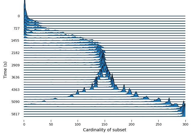
We show this in Figure 7, where we illustrate the distribution of for the first 300 images in the training dataset , observed over time in a run exhibiting the characteristic trajectory mentioned earlier. We notice that after some time, every image belongs to a group of size 150, which is half of the data points. This indicates the existence of two internally consistent subsets of images. This state persists for a while, after which one subset starts shrinking while the other grows until it encompasses all data points. The moment one subset begins to shrink and the other to grow coincides with the decrease in MSE.
Projective plane visualization
To explore the convergence process of the encoder, we developed a way to visualize the way in which the encoder predicts poses on the projective plane.
Let represent the set of images from a cryo-EM experiment. We define the equivalence relation on such that if and only if there exists some where (where is the left action of , see footnote 1). This relation leads to the formation of the set of equivalence classes .
Since each image in corresponds to an element in SO(3), each element in can be seen as part of the real projective plane P SO(3)/O(2). The projective plane can be imagined as the unit sphere where each pair of opposite points is identified. Recall that each image has a corresponding pose in SO(3), with being the axis of projection in the image formation process, also known as the ‘viewing direction’. Each equivalence class in then corresponds to a point on the projective plane, where the viewing direction is one of such paired points.
We make the projective plane visualizations as shown in Figure 8, by projecting poses onto the xy-plane as shown after first aligning them with the ground truth poses in the same way as we would to to determine the MSE (see F). We do this for both the ground truth poses and the poses predicted by the encoder. To visualize how the predicted poses differ from their ground truth pose, we color each of the predicted poses with the color that their corresponding ground truth pose has according to a colormap on the xy-plane.
In Figure 10(a) and Figure 9(a) we show examples of patterns in the projective plane visualizations that occur for the different datasets in states where the MSE is high, and the MedSE is low. For both structures, a pattern is observable where approximately half of the point are mirrored with respect to some line in the xy-plane. From these patterns in the projective plane alone, interpreting how the encoder misclassifies subsets of poses is challenging. However, the patterns indicate that the internally consistent subsets of data points are sometimes distinguishable within the projective plane.
Ground truth poses
Pattern 2 of predicted poses
[0.3]![[Uncaptioned image]](/html/2406.01630/assets/Figures/gt.jpg) [0.3]
[0.3]![[Uncaptioned image]](/html/2406.01630/assets/Figures/pattern1.jpg) [0.3]
[0.3]![[Uncaptioned image]](/html/2406.01630/assets/Figures/pattern2.jpg)
Pattern 1 of predicted poses
Ground truth poses
[0.3]![[Uncaptioned image]](/html/2406.01630/assets/Figures/gt.jpg) [0.3]
[0.3]![[Uncaptioned image]](/html/2406.01630/assets/Figures/pattern3.jpg)
Pattern of predicted poses
Spurious planar symmetries
In addition, the discussed states corresponded to the decoder reconstructing volumes that have a spurious planar symmetry. In Figure 11(a) we show reconstructions with such symmetries together with to their corresponding ground truth volumes. This phenomenon that is also discussed in Levy et al. (2022a), in which it was shown that a symmetric loss function prevents the model from getting stuck in states showing these symmetries. Our exploration shows that even with a symmetric loss function, these states occur.
Spliceosome structure
80S ribosome structure
[.40]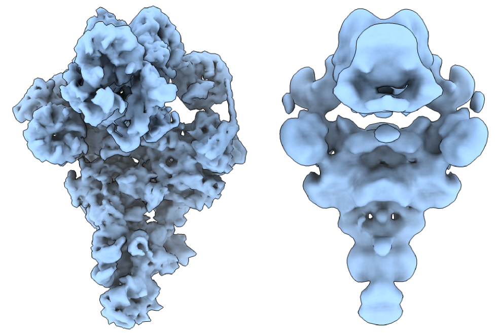 [.47]
[.47]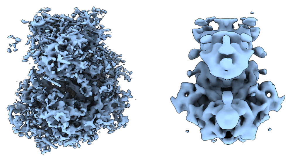
Upon comparing the reconstructions showing planar symmetry with the projective plane visualizations as shown in Figure 9(a) and Figure 10(a), we find that for the patterns in which a subset of points is mirrored with respect to a line in the xy-plane, this line corresponds to the plane of symmetry of the reconstructed volume.
We hypothesize that the patterns in the projective plane and the planar symmetry in the reconstructed volume can be explained by the fact that for volumes that have a planar symmetry, some viewing directions yield very similar projections, even though they would yield different projections in a non-symmetric volume. We show an example of this in Figure 12(a). This enables the pipeline to reconstruct images in the dataset with a low loss in two disctinct ways. The pipeline in stuck in a state reconstructing a volume with planar symmetry when the encoder is equally likely to predict each of these two. This explains the two equally sized internally consistent subsets of poses.
Reconstructed volume
Projection with viewing direction (B).
Ground truth volume
Projection with viewing direction (B).
[0.49]
[]![[Uncaptioned image]](/html/2406.01630/assets/Figures/symmetry/image19_1_.png)
[0.45]![[Uncaptioned image]](/html/2406.01630/assets/Figures/symmetry/image28.png) [0.45]
[0.45]![[Uncaptioned image]](/html/2406.01630/assets/Figures/symmetry/image26.png) [0.49]
[]
[0.49]
[]![[Uncaptioned image]](/html/2406.01630/assets/Figures/symmetry/image20_1_.png)
[0.45]![[Uncaptioned image]](/html/2406.01630/assets/Figures/symmetry/image34.png) [0.45]
[0.45]![[Uncaptioned image]](/html/2406.01630/assets/Figures/symmetry/image33.png)
Projection with viewing direction (A).
Projection with viewing direction (A).
Interpretation of results
The cryoAI authors (Levy et al. (2022a)) have noted that without a symmetric loss function, the pipeline could remain in local minima featuring reconstruction showing spurious planar symmetries for extended periods. We find that even with a symmetric loss function, the standard model can temporarily get stuck in similar local minima. In these states, due to planar symmetry, two distinct poses can generate the same projection, unlike in non-symmetric volumes. The exploratory study also reveals that when the model is in a state reconstructing a symmetric volume, the poses predicted by the encoder form two equally sized groups, each internally consistent but inconsistent with each other. We hypothesize that these groups represent the two distinct ways of generating the same projection in a volume showing spurious planar symmetry.
We hypothesize that the symmetric loss helps the model escape states in which it is reconstructing volumes with spurious planar symmetries as follows. Utilizing a symmetric loss function involves augmenting each batch with a rotated (or in the case of a mirror loss, mirrored) duplicate of each image in the batch. Both versions of the image pass through the model, but the model is only supervised on the best reconstruction. Recall that we observed that, when reconstructing a volume showing a spurious planar symmetry, two distinct poses can generate the same projection. We expect that at least sometimes, rotating (or mirroring) an image causes the encoder to switch from predicting one pose to the other that can generate the same projection. If, by chance, one aspect of the symmetry in the reconstructed volume provides marginally better reconstructions for a specific image, the model may begin to prefer this aspect, and as such ‘escape’ the symmetric state.