Magnetically generated spin-orbit coupling for ultracold atoms with slowly varying periodic driving
Abstract
The spin-orbit coupling (SOC) affecting the center of mass of ultracold atoms can be simulated using a properly chosen periodic sequence of magnetic pulses. Yet such a method is generally accompanied by micro-motion which hinders a precise control of atomic dynamics and thus complicating practical applications. Here we show how to by-pass the micro-motion emerging in the magnetically induced SOC by switching on and off properly the oscillating magnetic fields at the initial and final times. We consider the exact dynamics of the system and demonstrate that the overall dynamics can be immune to the micro-motion. The exact dynamics is shown to agree well with the evolution of the system described by slowly changing effective Floquet Hamiltonian including the SOC term. The agreement is shown to be the best when the phase of the periodic driving takes a specific value for which the effect of the spin-orbit coupling is maximum.
I Introduction
Spin-orbit coupling (SOC) manifests for electrons in solids Winkler (2003), where manipulation of electron spins by SOC plays an important role for spintronics and quantum information processing. During the last decade there has been also a great deal of interest in SOC for ultracold atoms Ruseckas et al. (2005); Stanescu et al. (2007); Juzeliūnas et al. (2008); Lin et al. (2011); Goldman et al. (2014); Zhai (2015); Galitski et al. (2019); Burba et al. (2024). The SOC can lead to novel many-body phases for ultracold atoms Goldman et al. (2014); Zhai (2015); Galitski et al. (2019) and offer applications in areas like spintronics Vaishnav et al. (2008); Madasu et al. (2022) and precision measurements Mamaev et al. (2021); Hernández Yanes et al. (2022)
The SOC affecting the center of mass of ultracold atoms is usually created by applying laser fields inducing transitions between the atomic internal states accompanied by the recoil Ruseckas et al. (2005); Stanescu et al. (2007); Juzeliūnas et al. (2008); Lin et al. (2011); Goldman et al. (2014); Zhai (2015); Galitski et al. (2019). This provides an effective coupling between the atomic spin and linear momentum. Alternatively the SOC can be simulated by means of a properly chosen periodic sequence of magnetic pulses Anderson et al. (2013); Xu et al. (2013), and the method has been implemented for rubidium and sodium atoms Luo et al. (2016); Shteynas et al. (2019). Specifically, by applying to ultracold atoms an oscillating magnetic field with a spatial gradient and an additional pulsed magnetic field, one can simulate an effective spin-orbit coupling similar to the one induced by laser fields. The magnetic-based approach can provide fast and flexible changes of the system parameters, such as the recoil momentum. This can be useful for controlling and manipulating of atomic spin states.
The SOC created by the oscillating magnetic field is generally accompanied by micro-motion which hinders a precise control of atomic dynamics and thus complicates applications. These include a fundamental study of the generation of topological states Goldman et al. (2014); Atala et al. (2014); Mamaev et al. (2022), subwavelength lattices Anderson et al. (2020); Burba et al. (2023), non-trivial quantum correlations like spin sqeezing Mamaev et al. (2021); Hernández Yanes et al. (2022, 2023) or indirectly Bell correlations Płodzień et al. (2022).
Here, we show how to by-pass the micro-motion emerging in the magnetically induced SOC by switching on and off properly the oscillating magnetic fields at the initial and final times. We consider the exact dynamics of the system from the initial to the final times and demonstrate that the overall dynamics can be immune to the micro-motion. Furthermore the exact dynamics agree well with the evolution of the system described by the slowly changing effective Floquet Hamiltonian which contains the SOC term. The agreement is the best when the phase of the periodic driving takes a specific value for which the effect of the spin-orbit coupling is maximum. In that case, the first-order effective Floquet Hamiltonian vanishes and the zero-order Floquet Hamiltonian is correct up to the second-order expansion in the inverse powers of the driving frequency. In this way, our results provide evidence that the magnetically induced SOC can be generated in a controllable way without involving the micro-motion.
The reduction of the micro-motion effect opens the path for the SOC implementation in systems where the Raman coupling is difficult to apply, for example for light atoms like lithium for which the fine structure splitting responsible for the SOC is very small. In that case the Raman transitions inducing the SOC should be very close to the excited state resonance in order to resolve the fine structure, which might be lead to significant losses. The magnetically generated SOC does not rely on the fine structure splitting and thus provides a method for creating the SOC for a wide range of atoms including the light ones.
II Formulation
II.1 Hamiltonian
We will consider spinful atoms affected by a time-dependent inhomogeneous magnetic field. The atomic Hamiltonian can then be separated into a spin-independent (SI) and a spin-dependent (SD) parts:
| (1) |
The former SI contribution includes operators for kinetic energy for the atomic motion in the direction and spin-independent (SI) potential which can represent any SI potential, such as a parabolic trap or an optical lattice:
| (2) |
where and are the atomic position and momentum operators, being the atomic mass.
On the other hand, the SD terms reads
| (3) |
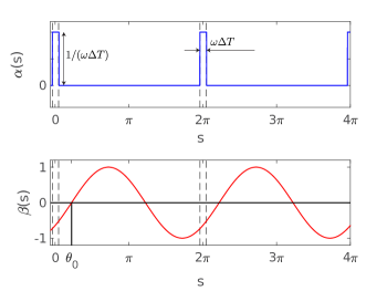
where (with ) are the Cartesian components of the spin operator . The first term in Eq. (3) represents the spin-dependent linear potential slope due to inhomogeneous magnetic field along the axis. It is characterized by a slowly changing dimensionless amplitude and a periodic part oscillating with a frequency . As illustrated in Fig. 1, the latter function is taken to be sinusoidal with a tunable phase :
| (4) |
The second term in Eq. (3) includes a possible detuning between the neighboring spin projection states. The third term is due to a pulsed Zeeman field oriented along the axis. The Zeeman term is characterised by a slowly changing dimensionless amplitude and a periodic part . The latter has large non-zero values only for a short temporal duration around multiple integers of the driving period (see Fig. 1), where is an integer, and each peak is normalized to unity,
| (5) |
For example, can be composed of a series of square potentials of a temporal width :
| (6) |
A specific condition how short should be the Zeeman pulses is presented in Appendix A.2. In writing Eq. (3) we have introduced a wave-number and a Rabi frequency characterizing, respectively, the strength of the gradient and Zeeman fields.
The spin-dependent Hamiltonian of the form of Eq. (3) can be simulated using a setup which involves an oscillating quadrupole magnetic, a strong bias magnetic field along the quantisation axis , as well as an oscillating radio frequency magnetic field along the orthogonal () direction, see the Supplementary material of Ref. Shteynas et al. (2019).
In the previous studies Luo et al. (2016); Shteynas et al. (2019) the gradient and Zeeman field were considered to have constant temporal profiles, . In that case the temporal evolution of the periodically driven quantum system is sensitive to the choice of the initial and the final times due to the micromotion Goldman and Dalibard (2014); Eckardt and Anisimovas (2015); Novičenko et al. (2017). To avoid the effect of micromotion, here we introduce the slowly changing amplitudes of the oscillating gradient and Zeeman fields and which describe a smooth switching on and off of these fields. By setting these amplitudes to zero at the initial and final times, we demonstrate that the overall dynamics of the periodically driven system is not sensitive to the specific choice of the initial and final times, and is well described by the slowly changing effective Floquet Hamiltonian.
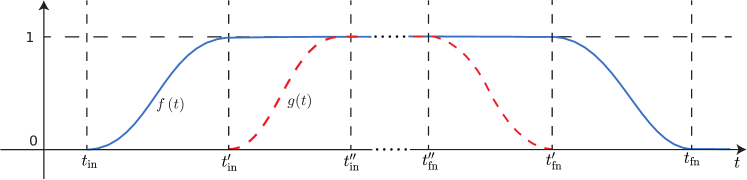
We will consider the following timing of the Zeeman and the gradient magnetic fields. Initially both fields are zero: for . The amplitude of the gradient field is ramped up slowly from at the initial time to a saturation value at the time , as illustrated schematically in Fig. 2. During the time interval the amplitude of the pulsed Zeeman field remains zero and is ramped up during the next time interval after the saturation of is reached, as one can see Fig. 2. The amplitudes are constant for and subsequently are ramped down in the opposite order. Specifically, the amplitude is ramped down first at and finally the amplitude goes to zero at , as illustrated in Fig. 2. The implications of such a timing for the ramping up and down of the periodic perturbation will be discussed next.
II.2 Elimination of the spin-dependent potential slope
The multiplier in the first term of Eq. (3) reflects the fact that by increasing the driving frequency the amplitude of inhomogeneous magnetic field is also increased. On the other hand, we are interested in the high-frequency limit where the frequency of the periodic driving exceeds all other characteristic frequencies featured in the Hamiltonian. This is not the case for the spin-dependent potential slope , so this term will be eliminated in the Hamiltonian (3) via a time-dependent unitary transformation
| (7) |
where
| (8) |
Here the lower integration limit is taken to be the initial time , so that
| (9) |
Thus the original and transformed representations coincide at the initial time . Both representations coincide also at the final time provided is a smooth function changing little within the driving period . Indeed in that case the function can be expanded as (see Appendix A.1)
| (10) |
so, using , one finds that
| (11) |
As the amplitude changes little within the driving period (, , etc.), for the present purposes it is sufficient to keep only the zero order term in Eq. (10), giving
| (12) |
The transformed Hamiltonian reads
| (13) |
where the transformed spin operator describes spin rotation around the axis:
| (14) |
The periodic function multiplying in the Hamiltonian of Eq. (13) is non-zero only in a narrow vicinity of multiple integers of the driving period . Therefore one can replace by in Eq. (14) for , see Appendix A.2 for estimating an error. Furthermore, since the function reaches its saturation value when is still zero, one can put in entering , so that one can make the following replacement in the Hamiltonian of Eq. (13)
| (15) |
with
| (16) |
The amount of spin rotation is thus determined by the the wave-number times the distance .
III Exact and effective evolution
III.1 Effective Floquet Hamiltonian
In the original Hamiltonian given by Eqs. (1)-(3) the periodic perturbation represents the spin-dependent potential slope proportional to . In the transformed Hamiltonian given by Eq. (13) this term is eliminated, and the oscillating perturbation is no longer proportional to the driving frequency . The atomic dynamics can then be well described in terms of a slowly changing effective Floquet Hamiltonian which can be expanded in the powers of the inverse driving frequency , a procedure known as the high frequency expansion Novičenko et al. (2017):
| (17) |
where the th term is proportional to . We will restrict to the first two terms given by
| (18) | ||||
| (19) |
where are slowly changing operators featured in the Fourier expansion of the time-periodic Hamiltonian with respect to the first argument :
| (20) |
Since given by Eq. (10) is expanded in the inverse powers of , the Fourier components can also be expanded in the powers of , i.e. . In the present situation , so it is sufficient to keep only the leading term of given by Eq.(12) when considering and .
The Fourier component providing the zero-order effective Floquet Hamiltonian is obtained by averaging the Hamiltonian with respect to the rapidly changing argument . According to Eq. (10), the function averages to zero , and the average of its square is Furthermore, according to Eq. (5), averages to the unity over the period. Thus, using Eqs. (13) and (16) for , the slowly changing zero-order effective Floquet Hamiltonian reads:
| (21) |
In what follows we will consider the case of the spin 1/2 for which the Cartesian components of the spin operator read (with ), where are the Pauli matrices. In that case , so the last term of Eq.(21) is spin independent and represents the slowly changing shift in the origin of energy. As demonstrated in Appendix B, for the spin-1/2 one can make simplifications also to the first order effective Hamiltonian leading to the following result:
| (22) |
where is given by
| (23) |
Note that the first order contribution to the effective Hamiltonian reduces to zero for the most interesting situation where , in which the momentum of spin-orbit coupling is maximum and the condition (41) holds the best, as discussed below. In that case the zero-order effective Hamiltonian describes effectively the evolution of the system up to the terms quadratic in the inverse frequency .
The operators and change slowly in time due to slow changes of the amplitudes of the gradient and Zeeman fields and . The spin rotation term in Eq. (21) for the effective Hamiltonian represents the spin orbit coupling (SOC) characterised by the slowly changing strength and the wave-number of the momentum transfer . The wave-number is determined by the phase between the gradient and the pulsed Zeeman fields, like in the stationary case where Shteynas et al. (2019). The momentum transfer is maximum and equals to for when the spikes of the infrared Zeeman field are situated at zeros of the gradient field. In that case the condition (41) holds best, and also there is no first order contribution to the effective Hamiltonian, . On the other hand, the momentum transfer is zero for when the spikes of the Zeeman field coincide with maxima/minima of the gradient field.
III.2 Dynamics of the system
The overall dynamics of the state vector of the system from the initial to the final times governed by the slowly changing periodic Hamiltonian is described by the evolution operator
| (24) |
where signifies the time-ordering. The operator can be represented in terms of the effective evolution operator due to the slowly changing effective Hamiltonian and the micromotion operators and calculated at the initial and final times and Novičenko et al. (2017):
| (25) |
Here the effective evolution is given by
| (26) |
and the micromotion operator reads up to the terms linear in :
| (27) |
The operator describes effects due to the fast changes of the Hamiltonian . It goes to the unity when periodic driving switches off Novičenko et al. (2017). Thus in the present situation the micromotion operator reduces to the unity for and . In this way, the overall dynamics described by the slowly changing effective Floquet Hamiltonian should reproduce well the exact dynamics governed by the exact Hamiltonian . An additional temporal dependence is due to the time-dependent unitary operator transforming the original state vector to the new representation. Yet, the transformation given by Eq. (7) reduces to the unity at the initial and final times and thus does not affect the overall evolution of the system from the initial to the final times. Therefore one can consider the time evolution from the initial to the final times governed by the transformed Hamiltonian , which is turn can be described by the slowly changing effective Floquet Hamiltonian , i.e.
| (28) |
In the next Subsection we will make sure that this is the case.
In the stationary regime where the effective Floquet Hamiltonian (21) becomes time-independent and is given by for the case of spin 1/2
| (29) |
with .
The effective Hamiltonian given by Eq. (21) or (29) is analogous to the light induced coupling between the (quasi-) spin up and down states accompanied by the recoil , like the one used to study the spin squeezing in optical lattices Hernández Yanes et al. (2022). The Hamiltonian reduces to the SOC involving coupling between the linear momentum and the spin component via the unitary transformation Lin et al. (2011). Note also that the effective Hamiltonian (21) or (29) has been derived under the high frequency assumption implying that the driving frequency is larger than all the frequencies associated with the time-periodic Hamiltonian changing slowly within the driving period. In that case the effective Hamiltonian reproduces very well the exact evolution, as we will see next.
III.3 Exact vs numerical results
We will compare the time evolution of the time-dependent Schroedinger equation (TDSE), calculated numerically for both cases: the exact time-periodic Hamiltonian and the effective Hamiltonian . The two component (spinor) wavefunctions and governed by and , respectively, are chosen to be the same at the initial time, . Both spinor wave functions should be almost identical at the final time, , if the high frequency conditions are met: , , , Additionally, the duration of the Zeeman pulses should be small enough compared to the driving period , so there is an extra condition following from (41) in Appendix A.2: , where the sample length is taken to be much larger than the inverse momentum , i.e. . The condition (v) is satisfied in the experiment Shteynas et al. (2019) where the sample length is of the order of m, the wave-number of the order of and . Note that the condition holds best if the phase difference is zero: , i.e. when the spikes of the Zeeman field are situated at zero points of the profile . In that case the condition (v) reduces to .
In the numerical calculations, we will assume that the atoms are confined in a square well with infinitely high potential boundaries at and zero potential for . The ramping functions and are taken to have the following form
| (30) |
| (31) |
where is the time interval between the ramping on and off, is the ramping time of the periodic driving and is the time delay between the ramping of the functions and . By taking we choose , , and similarly , , . In that case we have and , as well as and , as illustrated in Fig. 2.
Note that according to the condition (iv) presented at the beginning of Sec. III.3, the ramping rate should be much smaller the driving frequency . On the other hand, the ramping time should be smaller than the decoherence time . The latter condition can not be met in the experiment of ref. Shteynas et al. (2019) in which the decoherence time is of the order of 1 ms whereas driving period is only around 10 times smaller. To satisfy the slow ramping condition, one should increase the decoherence time, which is expected to be done in the future experiments. In the subsequent plots displayed in Fig. 3 and Fig. 4 the ramping rate is taken to be 100 times smaller than the driving frequency, which can be applied to future experiment with the relative decoherence times larger than that in Ref. Shteynas et al. (2019).
III.3.1 Comparison of exact and effective dynamics
To compare the dynamics, we will look at the inner product between the state vectors and evolving, respectively, by the exact time periodic Hamiltonian and the effective slowly changing Hamiltonian :
| (32) |
If the inner product is unity for , the overall dynamics of the two state-vectors is equivalent. Otherwise, this is not the case. Thus for numerics, one may look at and . Deviations of these quantities from and , respectively, signify differences between the state-vectors and thus, the non-equivalence of the dynamics. We will explore this differences for state-vectors characterized by three orthogonal initial spin polarizations. For this we introduce the following functions:
| (33) |
| (34) |
where once again, deviations of these functions from and signify differences between the state-vectors.
Specifically, the spatial part of the initial state vectors is taken to be an eigenstate of the box potential , and the spin is pointing along the , and axis:
| (35) |
where:
| (36) |
and
| (37) |
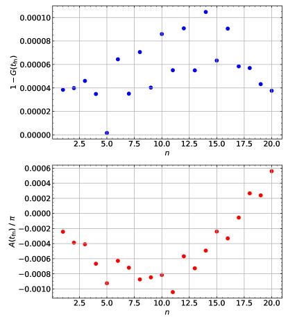
The functions and are presented in Fig. 3. One can see that and . This shows that for the overall dynamics from the initial to the final times is well described in terms of the effective dynamics governed by the zero order effective Hamiltonian. Indeed the first-order effective Hamiltonian presented in Eq. (22) goes to zero for , where is an integer number. Additionally, due to adiabatic ramping described by the ramping functions and , the effects of micro-motion disappear at the initial and and final times in the plots displayed in Fig. 3 and in the subsequent Fig. 4. Therefore, for , the approximate dynamics given by the zero-order effective Hamiltonian , is accurate up to second order in the inverse frequency.
III.3.2 First-order correction effect
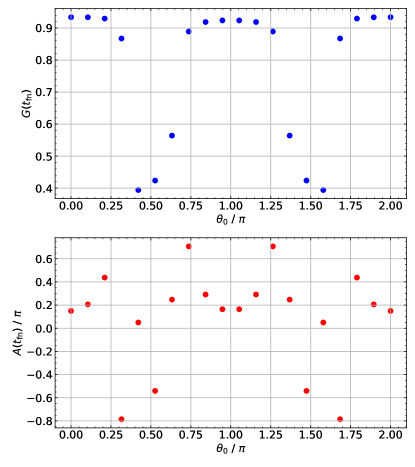
If , the first order effective Hamiltonian is no longer zero, and the approximate dynamics is accurate only up to first order in the inverse frequency. In Fig. 4 we have demonstrate the difference in the approximation accuracy for various by calculating the dependence of on . One can see clearly that the approximation holds best for for which . Here we have deliberately chosen the driving frequency to be considerably smaller than the one used in other plots, so that one can more clearly see the relative importance of first order correction term .
IV Concluding remarks
We have demonstrated how to by-pass the micro-motion emerging in the magnetically induced SOC by switching on and off in a proper way the oscillating magnetic fields at the initial and final times. We have studied the exact dynamics of the system from the initial to the final times governed by the time periodic Hamiltonian and compared it to the dynamics described by the slowly changing effective Floquet Hamiltonian. The two dynamics agree well under the assumption of the high frequency driving. The agreement is shown to be the best when the phase of the periodic driving takes a specific value for which the effect of the spin-orbit coupling is maximum. In that case the first-order effective Floquet vanishes and the zero-order Floquet Hamiltonian is correct up to the second order expansion in the inverse powers of the driving frequency. The overall dynamics is thus well described by the slowly changing zero-order effective Floquet Hamiltonian containing the SOC term. In this way, the magnetically induced SOC can be induced in a controllable way without involving the micro-motion. This opens the path for practical applications of magnetically generated SOC, e.g. generation of nontrivial topological or spin-squeezed states for ultracold atoms in optical lattices, when the optically generated SOC is complicated to apply.
Acknowledgements.
This work was supported by the European Social Fund (Project No. 09.3.3-LMT-K-712-23-0035) under a grant agreement with the Research Council of Lithuania (M.M.S.).Appendix A Analysis of
A.1 Function
Let us now find out how to separate a fast periodic time dependence of from its additional slow temporal dependence. To that end, we expand as a series of terms, where denotes an -th order temporal derivative of the slowly varying envelope function . Substituting Eq. (4) into (7) and integrating by parts, one finds
| (38) |
This provides an expansion in a series of terms proportional to :
| (39) |
where we used the fact that .
A.2 Estimation of error
To estimate an error made in writing Eq. (16) for , let us expand the function given by Eq. (10) in the powers of around a spike centered at , with an integer . Since amplitude reaches its stationary value when is still zero, one finds up to the quadratic term by putting :
| (40) |
Therefore the maximum displacement at which is still non-zero yields the following maximum value of :
| (41) |
Since , then .
Equation (16) is valid if
| (42) |
where is a characteristic size of the atomic cloud. The conditions (42) holds best if the phase difference is zero: , i.e. when the spikes of the Zeeman field are situated at zero points of the profile . In that case is quadratic in , and the condition (42) reduces to:
| (43) |
Equations (41)-(42) or (43) provide restrictions on the size of the atomic cloud . Since , the width of the spikes should be sufficiently small compared to the driving period .
Appendix B First-order effective Hamiltonian
Here will provide explicit calculations of the first-order effective Hamiltonian in the transformed frame. The general formula for the first-order effective Hamiltonian is presented by Eq. (22):
| (44) |
where are the Fourier components of the transformed Hamiltonian with respect to the first argument . The latter is given by Eq. (13):
| (45) |
Using the approximate expression (12) for , one has: . Thus the non-zero Fourier modes of with read:
| (46) |
Since the amplitude is composed of sharp peaks at , the Fourier components weakly depend on and can be written: for any .
Next let us analyse the specific Fourier components contributing to the effective Hamiltonian (44).
B.1 Contribution by Fourier modes
Fourier components with are:
| (47) |
The corresponding commutator featured in the effective Hamiltonian (44) reads:
| (48) |
The commutator may be rewritten as:
| (49) |
where
| (50) |
Using and , one obtains:
| (51) |
where
| (52) |
In what follows we will consider the case of the spin-1/2. In that case one has , so one can make further simplifications using . Consequently the commutator featured in Eq. (48) reduces to
| (53) |
Substituting Eq. (53) to Eqs. (48) and (44), one arrives at the first order effective Hamiltonian given by Eq. (22) in the main text.
B.2 Contribution by Fourier modes
Noting that:
| (54) |
the Fourier modes with read:
| (55) |
For spin-1/2 one has , so the last term of Eq. (55) is proportional to the identity operator, and the commutator reduces to zero. For arbitrary spin, the commutator is no longer zero and the first-order effective Hamiltonian would be more complicated.
B.3 Contribution by Fourier modes with
The Fourier with are all the same:
| (56) |
so the commutators vanish for .
B.4 Final result
References
- Winkler (2003) R. Winkler, Spin–Orbit Coupling Effects in Two-Dimensional Electron and Hole Systems (Springer, Berlin, 2003).
- Ruseckas et al. (2005) J. Ruseckas, G. Juzeliūnas, P. Öhberg, and M. Fleischhauer, Phys. Rev. Lett. 95, 010404 (2005).
- Stanescu et al. (2007) T. D. Stanescu, C. Zhang, and V. Galitski, Phys. Rev. Lett. 99, 110403 (2007).
- Juzeliūnas et al. (2008) G. Juzeliūnas, J. Ruseckas, M. Lindberg, L. Santos, and P. Öhberg, Phys. Rev. A 77, 011802(R) (2008).
- Lin et al. (2011) Y.-J. Lin, K. Jiménez-García, and I. B. Spielman, Nature 471, 83 (2011).
- Goldman et al. (2014) N. Goldman, G. Juzeliūnas, P. Öhberg, and I. B. Spielman, Rep. Progr. Phys. 77, 126401 (2014).
- Zhai (2015) H. Zhai, Rep. Prog. Phys. 78, 026001 (2015).
- Galitski et al. (2019) V. Galitski, G. Juzeliūnas, and I. B. Spielman, Phys. Today 72, 38 (2019).
- Burba et al. (2024) D. Burba, H. Dunikowski, M. R. de Saint-Vincent, E. Witkowska, and G. Juzeliūnas, “Effective light-induced hamiltonian for atoms with large nuclear spin,” (2024), arXiv:2404.12429 [quant-ph] .
- Vaishnav et al. (2008) J. Y. Vaishnav, J. Ruseckas, C. W. Clark, and G. Juzeliūnas, Phys. Rev. Lett. 101, 265302 (2008).
- Madasu et al. (2022) C. S. Madasu, M. Hasan, K. D. Rathod, C. C. Kwong, and D. Wilkowski, Phys. Rev. Res. 4, 033180 (2022).
- Mamaev et al. (2021) M. Mamaev, I. Kimchi, R. M. Nandkishore, and A. M. Rey, Phys. Rev. Res. 3, 013178 (2021).
- Hernández Yanes et al. (2022) T. Hernández Yanes, M. Płodzień, M. Mackoit Sinkevičienė, G. Žlabys, G. Juzeliūnas, and E. Witkowska, Phys. Rev. Lett. 129, 090403 (2022).
- Anderson et al. (2013) B. M. Anderson, I. B. Spielman, and G. Juzeliūnas, Phys. Rev. Lett. 111, 125301 (2013).
- Xu et al. (2013) Z.-F. Xu, L. You, and M. Ueda, Phys. Rev. A 87, 063634 (2013).
- Luo et al. (2016) X. Luo, L. Wu, J. Chen, Q. Guan, K. Gao, Z.-F. Xu, L. You, and R. Wang, Scientific Reports 6, 18983 (2016).
- Shteynas et al. (2019) B. Shteynas, J. Lee, F. C. Top, J.-R. Li, A. O. Jamison, G. Juzeliūnas, and W. Ketterle, Phys. Rev. Lett. 123, 033203 (2019).
- Atala et al. (2014) M. Atala, M. Aidelsburger, M. Lohse, J. T. Barreiro, B. Paredes, and I. Bloch, Nature Physics 10, 588 (2014).
- Mamaev et al. (2022) M. Mamaev, T. Bilitewski, B. Sundar, and A. M. Rey, PRX Quantum 3, 030328 (2022).
- Anderson et al. (2020) R. P. Anderson, D. Trypogeorgos, A. Valdés-Curiel, Q.-Y. Liang, J. Tao, M. Zhao, T. Andrijauskas, G. Juzeliūnas, and I. B. Spielman, Phys. Rev. Research 2, 013149 (2020).
- Burba et al. (2023) D. Burba, M. Račiūnas, I. B. Spielman, and G. Juzeliūnas, Phys. Rev. A 107, 023309 (2023).
- Hernández Yanes et al. (2023) T. Hernández Yanes, G. Žlabys, M. Płodzień, D. Burba, M. M. Sinkevičienė, E. Witkowska, and G. Juzeliūnas, Phys. Rev. B 108, 104301 (2023).
- Płodzień et al. (2022) M. Płodzień, M. Lewenstein, E. Witkowska, and J. Chwedeńczuk, Phys. Rev. Lett. 129, 250402 (2022).
- Goldman and Dalibard (2014) N. Goldman and J. Dalibard, Phys. Rev. X 4, 031027 (2014).
- Eckardt and Anisimovas (2015) A. Eckardt and E. Anisimovas, New J. Phys. 17, 093039 (2015).
- Novičenko et al. (2017) V. Novičenko, E. Anisimovas, and G. Juzeliūnas, Phys. Rev. A 95, 023615 (2017).