Effectiveness of denoising diffusion probabilistic models for fast and high-fidelity
whole-event simulation in high-energy heavy-ion experiments

Abstract

Artificial intelligence (AI) generative models, such as generative adversarial networks (GANs), variational auto-encoders, and normalizing flows, have been widely used and studied as efficient alternatives for traditional scientific simulations. However, they have several drawbacks, including training instability and inability to cover the entire data distribution, especially for regions where data are rare. This is particularly challenging for whole-event, full-detector simulations in high-energy heavy-ion experiments, such as sPHENIX at the Relativistic Heavy Ion Collider and Large Hadron Collider experiments, where thousands of particles are produced per event and interact with the detector. This work investigates the effectiveness of Denoising Diffusion Probabilistic Models (DDPMs) as an AI-based generative surrogate model for the sPHENIX experiment that includes the heavy-ion event generation and response of the entire calorimeter stack. DDPM performance in sPHENIX simulation data is compared with a popular rival, GANs. Results show that both DDPMs and GANs can reproduce the data distribution where the examples are abundant (low-to-medium calorimeter energies). Nonetheless, DDPMs significantly outperform GANs, especially in high-energy regions where data are rare. Additionally, DDPMs exhibit superior stability compared to GANs. The results are consistent between both central and peripheral centrality heavy-ion collision events. Moreover, DDPMs offer a substantial speedup of approximately a factor of 100 compared to the traditional Geant4 simulation method.

I Introduction

Simulating the interaction of particles with detectors in nuclear experiments is a computationally intensive task. The Monte Carlo (MC) method employed for this purpose involves tracking each particle’s interaction with the detector material. Software packages such as Geant4 [1] are commonly used, followed by digitization simulation. Calorimeter simulations are particularly time-consuming due to the large number of interaction steps induced by many secondary particles as they travel through the detector geometry. Simulating full-detector events with physics backgrounds can be even more computationally expensive. However, deep generative machine learning (ML) models have emerged as a promising alternative for faster simulations.

Deep generative neural networks learn a data distribution and create new data points implicitly sampling the learned distribution. There have been many different techniques developed over the past two decades. Auto-encoders [2] and variational auto-encoders [3] task neural networks to encode or compress data into lower-dimensional features in an embedding space and decode or expand the features back to the original ones. They sample new data by first sampling in the learned embedding space and decoding to the data space. Normalization flows [4, 5] draw random samples from a simple distribution and transform them to the target data distribution via a sequence of invertible and differentiable mappings. Generative adversarial networks (GANs) [6] set up a minimax game for two neural networks, a generator and a discriminator, competing against each other. The generator produces synthetic data from random samples, while the discriminator discerns the synthetic data from real ones. Once a balance is reached between the generator and the discriminator, one can sample new synthetic data using the trained generator. Recently, the Denoising Diffusion Probabilistic Model (DDPM) [7] and its variations [8, 9] have drawn attention for their stability in model training and high quality and diversity of the synthetic data. Meanwhile, contemporary text-to-image generative models [10], integrated with large language models, have introduced impactful artificial intelligence (AI) to various scientific domains [11, 12].

GANs have been successfully used to produce fast calorimeter simulations [13, 14, 15, 16, 17, 18, 19, 20, 21]. Diffusion models in calorimeter and other detector simulations also have been gaining popularity [22, 23, 24, 25, 26, 27, 28]. However, while most fast simulation algorithms are designed to handle single-shower simulations, research involving full-detector, whole-event ML simulations remains sparse. Full-detector simulations are essential in contexts such as heavy-ion collisions, where each event generates thousands of particles. They also play a key role in simulating the full-detector background, such as synchrotron radiation in detectors at the Electron-Ion Collider (EIC) [29] where millions of photons will have to be simulated per event despite rare detector hits. Typically, a large background sample is required for detailed signal simulation embedding. Due to the high complexity and computational requirements of these simulations, they present a significant challenge to the scientific community.

In high-energy heavy-ion collisions, there are highly nontrivial global correlations in the deposited energy, arising from phenomena like flow, minijets, or resonances/decays. Therefore, comprehensive, concurrent simulation of the entire event is imperative. Furthermore, numerous experiments measure rare and high-energy signals in the detector. This puts significant emphasis on the high-fidelity generation of rare features in both short- and long-distance scales, which poses a challenge for generative models.

This work introduces the first full-detector, whole-event heavy-ion simulation using DDPM and GAN models trained on the simulated calorimeter data from the sPHENIX [30, 31] experiment. The experimental background is discussed in Section II. The algorithm is explained in Section III, followed by the results and discussions in Sections IV and V, respectively.

II Problem Setting and Data Generation

The reference heavy-ion dataset used in this work is produced using the HIJING [32] MC event generator for Au+Au collisions at nucleon-nucleon center-of-mass energy ($\sqrt{\mathrm{s}_{\mathrm{NN}}}$) of $200\text{\,}\mathrm{G}\mathrm{e}\mathrm{V}$. The generated, long-lived particles then are subjected to a Geant4 simulation of the sPHENIX detector to model the effects of the detector. Events are generated with varying centrality and thereby exhibit distinct event characteristics. Specifically, two centrality ranges are used in this study: $0$–$10\%$ (referred to as “central” collisions) and $40$–$50\%$ (referred to as “mid-central” collisions), corresponding to larger and smaller medium sizes, respectively. In HIJING, the centrality is determined using the percentile of the impact parameter ($b$) between the colliding nuclei. The $b$-range of $0$–$4.88\ \mathrm{fm}$ ($9.71$–$10.81\ \mathrm{fm}$) corresponds to the centrality range of $0$–$10\%$ ($40$–$50\%$). In the generation, multiple simultaneous collisions in beam bunches, referred to as “pileup events,” are allowed.

The sPHENIX detector is equipped with three distinct calorimeters: electromagnetic (EMCal), inner hadronic (IHCal), and outer hadronic (OHCal) [33]. These calorimeters possess a uniform and hermetic acceptance within the pseudo-rapidity ($\eta$) range of $-1.1<\eta<1.1$, covering the entire azimuthal angle ($0<\phi<2\pi$). Each calorimeter is segmented into distinct, sensitive volumes called towers. The tower size of EMCal is $\Delta\eta\times\Delta\phi=0.025\times 0.025$, while the tower sizes of IHCal and OHCal are $\Delta\eta\times\Delta\phi=0.1\times 0.1$. Consequently, the EMCal tower size is four times finer than that of the IHCal/OHCal towers in both $\eta$ and $\phi$ dimensions. For a given event, the energies deposited within $4\times 4$ EMCal towers (16 total towers) are aggregated with the energies deposited in individual IHCal and OHCal towers to match the tower sizes between the EMCal and HCal. This results in the formation of an integrated energy tower that comprises the three calorimeters. The number of integrated towers covered in these $\eta$ and $\phi$ ranges are 24 and 64, respectively. Figure 1 shows the event displays of the combined tower energies with the sPHENIX geometry, generated by HIJING and simulated through Geant4 (HIJING+G4). Subsequently, this combined energy information is used to construct an energy image within the $(\eta,\phi)$-plane as shown in Figure 2 for the events of $0\,$–$10\%$ and $40\,$–$50\%$, respectively. The images containing (24, 64) towers in $(\eta,\phi)$ per event serve as the ground truth samples for training the ML models. Each centrality class is trained separately because event characteristics vary across centrality classes. Approximately 600,000 events are used for training in each centrality class.

Figure 1: Display of tower energies (blue) deposited in the calorimeter system with the sPHENIX geometry for the $0$–$10\%$ (left) and $40$–$50\%$ (right) centrality ranges of example events. The center portion is an illustration of the tracking system that resides inside the calorimeters.

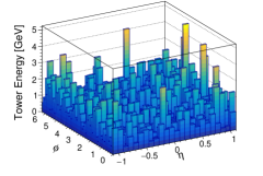
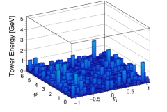
Figure 2: Tower energy distributions within the $(\eta,\phi)$-plane of the sPHENIX calorimeter system for the $0$–$10\%$ (top) and $40$–$50\%$ (bottom) centrality ranges of example events.

III Diffusion Models

Figure 3: Illustration of the forward and reverse diffusion processes. The forward process ($\mathbf{x}_{0}\to\mathbf{x}_{T}$) progressively adds Gaussian noise to an input image. The reverse process ($\mathbf{x}_{T}\to\mathbf{x}_{0}$) progressively denoises an image.

Diffusion models are a class of generative models [34], capable of producing novel data from random noise. This section reviews the DDPM model design and describes its training procedure.

III.1 The DDPM Model

The DDPM model [7] is built on the concept of a diffusion process (Figure 3) that has two directions: forward and reverse. The forward diffusion process takes a sample from the data distribution $\mathbf{x}_{0}\sim p_{\text{data}}$ and transforms it to look like a sample from the standard normal distribution $\mathcal{N}(\mathbf{0},\mathbf{I})$. The forward process is defined through a set of $T$ iterations, so-called diffusion steps, each of which adds a small amount of Gaussian noise to $\mathbf{x}_{0}$.

The reverse process takes a sample from the standard normal distribution $\mathbf{x}_{T}\sim\mathcal{N}(\mathbf{0},\mathbf{I})$ and transforms it back to the data distribution $p_{\text{data}}$. Similar to the forward process, the reverse diffusion process is defined through a set of $T$ iterations, or sampling steps, each of which is an inverse of the corresponding forward iteration. In effect, the reverse process removes the noise added in the forward steps. Thus, it is also referred to as the “denoising process.” Figure 3 illustrates both processes.

The reverse process can be used for data generation. To generate a data sample, one starts with a random noise $\mathbf{x}_{T}$ drawn from $\mathcal{N}(\mathbf{0},\mathbf{I})$. Then, one applies $T$ denoising iterations to $\mathbf{x}_{T}$ and obtains a sample $\mathbf{x}_{0}$. If the reverse process is correct, then $\mathbf{x}_{0}$ will be distributed according to $p_{\text{data}}$. In other words, the reverse process can be considered as a generative map that transforms the standard normal distribution $\mathcal{N}(\mathbf{0},\mathbf{I})$ into $p_{\text{data}}$.

Mathematically, the DDPM forward diffusion process is a Markov chain, where a single step is defined via Equation 1 [7]. The forward process is parameterized by a set of $\beta_{t}$ parameters, called a variance schedule. The variance schedule $\beta_{t}$ is treated as a set of hyperparameters of the DDPM model.

$$q(\mathbf{x}_{t}|\mathbf{x}_{t-1}):=\mathcal{N}\left(\mathbf{x}_{t};\sqrt{1-\beta_{t}}\mathbf{x}_{t-1},\beta_{t}\mathbf{I}\right)$$ (1)

A notable property of the Gaussian diffusion process is the existence of the closed-form expression for sampling $\mathbf{x}_{t}$ directly from $\mathbf{x}_{0}$ at an arbitrary time $t$, bypassing the whole iterative chain. Using the notation $\alpha_{t}:=(1-\beta_{t})$ and $\bar{\alpha}_{t}:=\prod_{s=1}^{s=t}\alpha_{s}$, it shows that $\mathbf{x}_{t}$ can be sampled from $\mathbf{x}_{0}$ according to Equation 2.

$$\mathbf{x}_{t}=\sqrt{\bar{\alpha}_{t}}\mathbf{x}_{0}+\sqrt{1-\bar{\alpha}_{t}}\mathbf{\epsilon}$$ (2)

where $\mathbf{\epsilon}\sim\mathcal{N}(\mathbf{0},\mathbf{I})$.

DDPM approximates the reverse process through a neural network $\mathbf{\epsilon}_{\theta}(\mathbf{x}_{t},t)$ [7]. This neural network is trained to predict the noise $\mathbf{\epsilon}$, added in the forward process (Equation 2), with a simple $L_{2}$ loss function (Equation 3)

$$\mathcal{L}(\theta):=\mathbb{E}_{\mathbf{x}_{0},t,\epsilon}\left[\left\|\mathbf{\epsilon}-\mathbf{\epsilon}_{\theta}\left(\sqrt{\bar{\alpha}_{t}}\mathbf{x}_{0}+\sqrt{1-\bar{\alpha}_{t}}\mathbf{\epsilon},t\right)\right\|_{2}^{2}\right]$$ (3)

Given the neural network $\mathbf{\epsilon}_{\theta}(\mathbf{x}_{t},t)$, it can be demonstrated that the reverse step is described by Equation 4.

$$\mathbf{x}_{t-1}=\frac{1}{\sqrt{\alpha_{t}}}\left(\mathbf{x}_{t}-\frac{1-\alpha_{t}}{\sqrt{1-\bar{\alpha}_{t}}}\mathbf{\epsilon}_{\theta}(\mathbf{x}_{t},t)\right)+\sigma_{t}\mathbf{z}$$ (4)

where $\mathbf{z}\sim\mathcal{N}(\mathbf{0},\mathbf{I})$ and $\sigma_{t}^{2}=\tilde{\beta}_{t}:=(1-\bar{\alpha}_{t-1})/(1-\bar{\alpha}_{t})\beta_{t}$. Experimentally, however, DDPM has shown [7] little difference between using $\sigma_{t}^{2}=\tilde{\beta}_{t}$ and $\sigma_{t}^{2}=\beta_{t}$. Therefore, we set $\sigma_{t}^{2}=\beta_{t}$ in this work.

The full DDPM model training (forward process) and data generation (reverse process) procedures are summarized in Table 1.

Algorithm 1 DDPM Training

1:repeat

2:     $\mathbf{x}_{0}\sim p_{\text{data}}$

3:     $t\sim\text{Uniform}(\{1,...,T\})$

4:     $\mathbf{\epsilon}\sim\mathcal{N}(\mathbf{0},\mathbf{I})$

5:     Perform Gradient Descent Step on   $\nabla_{\theta}\|\mathbf{\epsilon}-\mathbf{\epsilon}_{\theta}\left(\sqrt{\bar{\alpha}_{t}}\mathbf{x}_{0}+\sqrt{1-\bar{\alpha}_{t}}\mathbf{\epsilon},t\right)\|^{2}$

6:until converged

Algorithm 2 DDPM Sampling

1:$\mathbf{x}_{T}\sim\mathcal{N}(\mathbf{0},\mathbf{I})$

2:for $t=T,\;...\;,1$ do

3:     $\mathbf{z}\sim\mathcal{N}(\mathbf{0},\mathbf{I})\;\text{if}\;t>1,\;\text{else}\;\mathbf{z}=0$

4:     $\mathbf{x}_{t-1}=\frac{1}{\sqrt{\alpha_{t}}}\left(\mathbf{x}_{t}-\frac{1-\alpha_{t}}{\sqrt{1-\bar{\alpha}_{t}}}\mathbf{\epsilon}_{\theta}(\mathbf{x}_{t},t)\right)+\sigma_{t}\mathbf{z}$

5:end for

6:return $\mathbf{x}_{0}$

Table 1: DDPM training algorithm (left) and DDPM sampling algorithm (right) proposed in Ref. [7]

III.2 Factors Influencing DDPM Model Performance

There are several hyperparameters that influence the DDPM model performance. The first is the number of diffusion steps $T$. Empirically, larger $T$ is usually associated with a higher quality of the generated data [35, 8]. The second is the variance schedule $\beta_{t}$. The reference DDPM implementation [7] uses a linear schedule ($\beta_{t}\propto t$). However, the improved DDPM models (iDDPM) [35] have discovered that nonlinear variance schedules may perform better. Another important factor is the neural network architecture $\mathbf{\epsilon}_{\theta}(\mathbf{x}_{t},t)$. iDDPM has demonstrated that a few modifications to the DDPM network architecture may improve the DDPM model performance.

DDPM models are capable of generating very high-quality data, yet their exceptional performance comes at a high computational cost during model inference. According to the sampling algorithm (Algorithm 2), DDPM requires $T$ sequential neural network evaluations (also known as “sampling steps”) to generate a single image. This can make DDPM data generation prohibitively expensive. To speed up the inference, several approximate sampling algorithms have been developed for the DDPM model. Two of the simplest ones are the iDDPM [35] and DDIM [8] sub-sampling algorithms. Both algorithms allow one to perform a DDPM network evaluation at a smaller number of intermediate time steps. The smaller number of sampling steps enables a faster model inference at the cost of a small performance degradation. By default, we do not use the fast sub-sampling algorithms in this work, but we investigate the trade-offs between speed and performance in Section V.

III.3 DDPM Model Training

This effort relies on a reference implementation [36] of the diffusion network $\mathbf{\epsilon}_{\theta}(\mathbf{x}_{t},t)$ from the iDDPM work [35]. To find the optimal network configuration, we perform a sweep over several network parameters, including varying the depth/width of the model and using attention layers and scale-shift modulation.

Next, we experiment with using linear and cosine variance schedulers. The cosine variance schedulers result in poor-quality generated samples. Therefore, we use the linear variance scheduler throughout this work. For the linear scheduler, we conduct a sweep over the $\beta_{T}$ parameter to determine the best-performing values.

To further improve the model’s quality, we vary the number of diffusion steps $T$ and training epochs. The DDPM model performance responds positively to increasing both parameters. We set the number of diffusion steps to $T=$8000$$, sampling steps to $8000$, and training epochs to 500 as default because these values provide good generation quality while being small enough for efficient inference. The DDPM model response to the number of training epochs is described in Section IV.

Additionally, we have determined the best generation performance is achieved when the training data are normalized to the logarithmic scale. To perform such a normalization, we first clip the minimal data values by $1\text{\times}{10}^{-3}\text{\,}\mathrm{G}\mathrm{e}\mathrm{V}$ (minimum detector resolution) then apply natural logarithm normalization.

Finally, to assess the training stability, each DDPM model configuration is retrained with five random seeds. The variance of the model performance with different seeds is used to judge the training stability (cf. Section IV). Additional details, including the final network configuration and training procedure, can be found in Appendix A.1.

Figure 4: Calorimeter tower $E_{\mathrm{T}}$ distributions for HIJING+G4 (red circle), DDPM (blue lines), and GAN (yellow lines) in the $0$–$10\%$ centrality range (A) and the $40$–$50\%$ centrality range (B). The first four columns represent $E_{\mathrm{T}}$ of different tower areas: $1\times 1$, $4\times 4$, $7\times 7$, and $11\times 11$. The rightmost column is the distribution of total $E_{\mathrm{T}}$ per event ($\Sigma E_{\mathrm{T}}^{\mathrm{tower}}$). Bottom panels show the ratio of ML models to HIJING+G4. The five different lines for GAN and DDPM represent varied random seeds.

III.4 GAN Baselines

GANs [37] present an alternative family of generative models. Similar to the diffusion models, they offer the ability to synthesize high-quality data but with much faster inference times. In this work, we also explore GANs’ ability to generate samples for comparison with the DDPM model.

For the GAN baselines, we choose a widely used DCGAN model [38] and construct its generator and discriminator networks out of five DCGAN stages (with $2^{6}$, $2^{7}$, $2^{8}$, $2^{9}$, and $2^{10}$ channels per stage, respectively). The output of a DCGAN generator is an image of size $(64,64)$ pixels. Because the shape of the generated image does not match that of the towers $(24,64)$, we crop the image to the required shape. Similarly, the DCGAN discriminator expects an input image of shape $(64,64)$. To make the discriminator work on towers of $(24,64)$, we embed them into a larger $(64,64)$ image, initially filled with zeros.

Similar to the DDPM models, we find that a logarithmic data normalization gives better performance compared to an unaltered case. Likewise, all the final DCGAN configurations are retrained with five random seeds to assess their stability. The full training details of the GAN baselines are outlined in Appendix A.2. Despite numerous tuning attempts, the quality of the GANs-generated samples in this work is too poor for it to be considered a viable generation methodology. GANs also exhibit a high degree of training instability further limiting their applicability for high-fidelity generation. Additional details regarding the performance of the GANs and their comparison to the DDPM are discussed in Section IV.

Figure 5: Average standard deviation ($\langle\sigma^{E_{\mathrm{T}}}\rangle$) of calorimeter tower $E_{\mathrm{T}}$ as a function of $\Sigma E_{\mathrm{T}}^{\mathrm{tower}}$ for HIJING+G4 (red circle), DDPM (blue lines), and GAN (yellow lines) in the $0$–$10\%$ centrality range (A) and the $40$–$50\%$ centrality range (B). Bottom panels show the ratio of ML models to HIJING+G4. The five different lines for GAN and DDPM represent varied random seeds.

IV Results

The distribution of deposited calorimeter tower energies and its event-by-event fluctuation are compared between the HIJING+G4 and generated events by DDPMs and GANs to evaluate the efficacy of the ML models. A total of $100,000$ events are utilized for each dataset in this evaluation. The HIJING+G4 events used for evaluation is independent from HIJING+G4 events used for training. Figure 4A shows transverse energy ($E_{\mathrm{T}}$) distributions deposited in various calorimeter tower areas ($1\times 1$, $4\times 4$, $7\times 7$, and $11\times 11$) and the distribution of the total $E_{\mathrm{T}}$ of all towers ($\Sigma E_{\mathrm{T}}^{\mathrm{tower}}$) in the $0\,$–$10\%$ centrality range. The tower area is defined as the region occupied by the array of towers in the $\eta$ and $\phi$ direction. For example, a $7\times 7$ tower area consists of 49 towers. Both the DDPM and GAN models are trained five times with different random seeds to test stability. The DDPM has robust consistency across multiple seeds, whereas the GAN model shows significant fluctuations when varying seeds. The DDPM also offers a significantly more accurate description of HIJING+G4, typically within a few percentage points of accuracy where the distribution is populated, while the GAN fails to replicate the HIJING+G4, which is particularly evident at the distribution tails.

Figure 4B shows the calorimeter tower $E_{\mathrm{T}}$ distributions in the $40$–$50\%$ centrality range. Similar to the $0$–$10\%$ case, the DDPM outperforms the GAN in both the stability and better description of HIJING+G4. However, the DDPM starts to deviate from the HIJING+G4 at higher $E_{\mathrm{T}}$ regions, where the distribution displays a non-Gaussian structure. This structure likely arises from pileup events and minijets generated in HIJING, which occur rarely. The probability of encountering this high $E_{\mathrm{T}}$ tail at around $4\times 4$ tower $E_{\mathrm{T}}$ of 15 GeV is approximately $10^{-5}$, with only around $100$ occurrences contributing to this distribution in this evaluation.

In addition to the overall energy deposition, we examine energy fluctuations. The standard deviation of transverse energies ($\sigma^{E_{\mathrm{T}}}$) is calculated per event for different tower size configurations ($1\times 1$, $4\times 4$, $7\times 7$, and $11\times 11$ towers). The average $\sigma^{E_{\mathrm{T}}}$, $\langle\sigma^{E_{\mathrm{T}}}\rangle$, is shown as a function of $\Sigma E_{\mathrm{T}}^{\mathrm{tower}}$ in Figure 5A and Figure 5B for the $0$–$10\%$ and $40$–$50\%$ centrality ranges, respectively. Similar to the overall energy distributions, the DDPM provides significantly improved performance than the GAN and closely aligns with the HIJING across various tower configurations. This highlights the robust descriptive capability of the DDPM model.

V Discussion

Figure 6: Calorimeter tower $E_{\mathrm{T}}$ distributions in the $40$–$50\%$ centrality range with different numbers of training epochs (A) and sampling steps (B) of the DDPM. All curves in A are produced with 8000 sampling steps. All curves in B are produced with 4000 epochs.

Machine learning algorithms tend to work suboptimally when the training data are scarce. This is a significant problem in the context of high-energy heavy-ion collisions as the instances of large energy depositions are rare but essential for the overall fidelity of the simulation. The rare and large energy depositions often include high-energy phenomena, such as jets and photons, which are of scientific interest. To alleviate the problem and enhance fidelity, we increase the number of training epochs for the network to learn the distribution more accurately in less dense regions. Figure 6A shows that by increasing the training epochs, the DDPM works progressively better at the higher energy region of the distribution. It is important to note that increasing the number of epochs also prolongs the training time. In this work, each training session took 4 hours and 44 minutes per 100 epochs with the duration increasing linearly as the number of epochs rises. Therefore, there is a trade-off between the training time and quality with which rare features are reproduced.

The number of DDPM sampling steps also affects the time required to generate events. To explore the trade-offs between fidelity and generation speed, we have experimented with a fast sampling strategy proposed by iDDPM [35]. Figure 6B shows the impact of reducing the number of sampling steps from the default value of 8000 to 100. The DDPM model shows a steep improvement in generation quality as the number of sampling steps increases from $100$ to $1000$. Additional increases in the number of sampling steps bring progressively diminishing returns with $2000$ sampling steps providing similar performance to $8000$. This observation indicates that the generation speed can be improved by a factor of $4$ to $8$ without significant loss of quality. To further explore the possibilities of faster generation, we attempt to reevaluate the trained DDPM models in the DDIM mode [8]. However, DDIMs do not provide sufficient generation quality to be a viable alternative to the DDPM model. Additional details about generation with the DDIM model are discussed in Appendix B.

The average time to produce one event with HIJING and simulate it with Geant4 takes approximately 40 minutes using a single CPU core. Meanwhile, utilizing an NVIDIA RTX A6000 GPU, the GAN and DDPM with the denoising step of $8000$ require only about $0.42$ milliseconds and $1.34$ seconds, respectively. This represents a speedup of $5,700,000$ and $1800$ times faster than conventional event simulation. For a fair comparison between CPU and GPU, considering a $32$-core CPU equivalent to a GPU, the GAN and DDPM still offer a speedup on the order of $100,000$ and $100$, respectively. While the GAN demonstrates greater speed, the DDPM maintains high fidelity in describing the ground truth, which is crucial for scientific purposes.

In applications, there is a need for a large number of full-detector simulation events, such as those for heavy-ion collisions at RHIC and beam background events for the EIC detector. Rare signal events can then be embedded in these simulations. We envision using a relatively modest number (at the level of millions) of events simulated through Geant4 to train the diffusion model. Once trained, the model can be used to accelerate the production of much larger samples (at the level of billions) for signal embedding.

In addition to the tower $E_{\mathrm{T}}$ distributions and their fluctuations, there are more ways to characterize heavy-ion collisions and evaluate the performance of the generation, including tower correlations, azimuthal anisotropy and resonance (e.g. $\pi^{0}$) reconstruction, which is a subject for future work with larger statistics.

VI Summary

Simulating particle interactions with detectors in nuclear experiments is highly computationally demanding. This study introduces the first application of generative AI as an alternative to traditional simulation methods for full-event, whole-detector simulation of heavy-ion collisions. We employ both GANs and DDPM to generate events and compare them with the traditional method of HIJING+Geant4 simulation in detail. We find that the DDPM shows promise for high-fidelity and stable simulation in this application while maintaining orders of magnitude speed gain when compared with the traditional methods. This work demonstrates diffusion models are potentially useful tools for future full-detector, whole-event simulation campaigns in the nuclear physics field, such as experiments at the Relativistic Heavy Ion Collider, Large Hadron Collider, and future EIC.

Appendix A Training Details

This appendix summarizes various training details for the DDPM and GAN models used in the main paper.

A.1 DDPM Training Details

This work relies on a reference iDDPM implementation [36] of the diffusion network but changes its configuration. Our neural architecture is built from three U-Net encoder-decoder stages [39] (with 32, 64, and 128 channels per stage, respectively), each of which comprises two ResNet blocks [40]. This architecture is chosen as it gives good generation performance while not being overly complex. The iDDPM model allows one to incorporate attention layers into the U-Res-Net architecture. However, we did not observe any sizeable performance improvements with the inclusion of attention layers. Therefore, our network architecture is fully convolutional and does not use any attention layers. The scale-shift time modulation produces a slightly different effect, depending on the dataset. The DDPM shows better performance for the centrality 40–50% range with the scale-shift modulation, but the opposite is true for the centrality 0–10% dataset.

To further investigate performance of the DDPM models, we performed a hyperparameter sweep over the end value of the linear variance schedule $\beta_{T}\in(0.01,0.20)$. Our findings indicate that the DDPM performs best with $\beta_{T}=0.02$ for the centrality 40–50% range and $\beta_{T}=0.10$ for the centrality 0–10% range.

As the best DDPM model configurations differ between the datasets, we used different setups per dataset in the main paper:

• Centrality 0–10%: No scale-shift modulation, $\beta_{T}=0.02$

• Centrality 40–50%: Scale-shift modulation, $\beta_{T}=0.10$

Overall, the DDPM models are trained with a batch size of $128$. For consistency between different datasets, we limit the number of training steps per epoch to $2000$. For the default training (Figures 4, 5), the DDPM models are trained for $500$ epochs. To perform the additional investigations (Figures 6, 7) on the centrality 40–50% sample, we train the DDPM models for $4000$ epochs (unless otherwise indicated). The training was performed with the Adam optimizer [41] having a constant learning rate of $1\times 10^{-4}$.

A.2 GAN Training Details

The GANs used in this work are based on DCGAN architecture [38] and try to follow its training procedure closely. However, we found the default DCGAN training setup results yields significantly poor performance. To improve the situation, we experimented with using alternative loss functions and a gradient penalty (GP) term [42].

Specifically, we conducted hyperparameter sweeps over the choice of the loss function and use of the GP term [42]. For the loss function, we explored using the traditional binary cross entropy (BCE) loss function [37] (default DCGAN setup), WGAN-GP loss [42], and least squares GAN (LSGAN) loss [43]. For the GP configuration, we considered not using any gradient penalty (default DCGAN setup), using the original GP [42], and using the improved zero-centered GP term [44]. For each of the GP configurations, we also experimented with its magnitude $\lambda_{\text{GP}}$ from $\{1,10\}$.

Our findings indicate that the following configurations perform the best per dataset:

• Centrality 0–10%: Loss: WGAN-GP with the original GP of magnitude $\lambda_{\text{GP}}=1$.

• Centrality 40–50%: Loss: LSGAN with the original GP of magnitude $\lambda_{\text{GP}}=10$

These configurations are used in the main paper. All DCGAN models are trained with a batch size of $128$ (following the original DCGAN setup) for $1,000,000$ steps. We found no benefit in continuing the training further. For optimization, we used the Adam optimizer [41] with the learning rate of $1\times 10^{-4}$.

Appendix B DDPM Evaluation in DDIM Mode

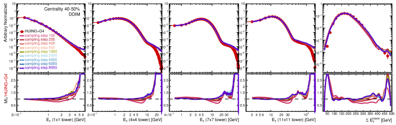
Figure 7: Calorimeter tower $E_{\mathrm{T}}$ distributions in the 40–50% centrality range with a different number of DDIM modesampling steps.

The DDIM [8] model provides an alternative formulation of the diffusion process. Unlike the DDPM model, the reverse process of DDIM is fully deterministic. This allows for establishing a 1-to-1 correspondence between the noise $\mathcal{N}(\mathbf{0},\mathbf{I})$ and the data $p_{\text{data}}$ distributions, which offers many interesting applications related to the modifications in the noise space [8, 45]. The DDIM also offers an alternative way of approximate inference that may outperform DDPM sub-sampling when the number of sampling steps is small [8].

The DDIM model’s training objective is constructed to match that of the DDPM model. This property permits us to reuse a trained DDPM model and evaluate it in a DDIM mode. Figure 7 shows the results of evaluating the DDPM models from the main paper in the DDIM mode.

Comparing DDIM inference (Figure 7) with the corresponding DDPM inference (Figure 6) of the same DDPM model, we observe a rather significant difference in the quality of the generated data. In particular, the DDIM performs poorly in the tails of the tower $E_{\mathrm{T}}$ distributions, irrespective of the number of sampling steps.

The especially poor performance of the DDIM model is relatively surprising given that it works well on natural images [8]. It is possible that the relatively better DDPM performance in the low-statistics region is due to the stochastic nature of the DDPM denoising process. The stochasticity of the denoising process may help to perturb initial samples enough to generate low-frequency data correctly. It is also possible that the DDIM’s underperformance stems from our models being optimized for DDPM performance, which may not align with optimizing for DDIM performance. Additional studies are necessary to differentiate the effects of DDIM determinism from the lack of optimization.

References

- Agostinelli et al. [2003] S. Agostinelli et al. (GEANT4), GEANT4–a simulation toolkit, Nucl. Instrum. Meth. A 506, 250 (2003).
- Hinton and Salakhutdinov [2006] G. E. Hinton and R. R. Salakhutdinov, Reducing the dimensionality of data with neural networks, science 313, 504 (2006).
- Kingma et al. [2019] D. P. Kingma, M. Welling, et al., An introduction to variational autoencoders, Foundations and Trends® in Machine Learning 12, 307 (2019).
- Rezende and Mohamed [2015] D. Rezende and S. Mohamed, Variational inference with normalizing flows, in International conference on machine learning (PMLR, 2015) pp. 1530–1538.
- Papamakarios et al. [2021] G. Papamakarios, E. Nalisnick, D. J. Rezende, S. Mohamed, and B. Lakshminarayanan, Normalizing flows for probabilistic modeling and inference, Journal of Machine Learning Research 22, 1 (2021).
- Goodfellow et al. [2014] I. Goodfellow, J. Pouget-Abadie, M. Mirza, B. Xu, D. Warde-Farley, S. Ozair, A. Courville, and Y. Bengio, Generative adversarial nets, Advances in neural information processing systems 27 (2014).
- Ho et al. [2020] J. Ho, A. Jain, and P. Abbeel, Denoising diffusion probabilistic models, Advances in neural information processing systems 33, 6840 (2020).
- Song et al. [2020a] J. Song, C. Meng, and S. Ermon, Denoising diffusion implicit models, arXiv preprint arXiv:2010.02502 (2020a).
- Song et al. [2020b] Y. Song, J. Sohl-Dickstein, D. P. Kingma, A. Kumar, S. Ermon, and B. Poole, Score-based generative modeling through stochastic differential equations, arXiv preprint arXiv:2011.13456 (2020b).
- Ramesh et al. [2022] A. Ramesh, P. Dhariwal, A. Nichol, C. Chu, and M. Chen, Hierarchical text-conditional image generation with clip latents, arXiv preprint arXiv:2204.06125 1, 3 (2022).
- Kazerouni et al. [2023] A. Kazerouni, E. K. Aghdam, M. Heidari, R. Azad, M. Fayyaz, I. Hacihaliloglu, and D. Merhof, Diffusion models in medical imaging: A comprehensive survey, Medical Image Analysis , 102846 (2023).
- Corso et al. [2023] G. Corso, H. Stärk, B. Jing, R. Barzilay, and T. Jaakkola, Diffdock: Diffusion steps, twists, and turns for molecular docking, in International Conference on Learning Representations (ICLR) (2023).
- Jaruskova and Vallecorsa [2023] K. Jaruskova and S. Vallecorsa, Ensemble Models for Calorimeter Simulations, J. Phys. Conf. Ser. 2438, 012080 (2023).
- Buhmann et al. [2021] E. Buhmann et al., Fast and Accurate Electromagnetic and Hadronic Showers from Generative Models, EPJ Web Conf. 251, 03049 (2021).
- Rehm et al. [2021] F. Rehm, S. Vallecorsa, K. Borras, and D. Krücker, Physics Validation of Novel Convolutional 2D Architectures for Speeding Up High Energy Physics Simulations, EPJ Web Conf. 251, 03042 (2021), arXiv:2105.08960 [hep-ex] .
- Khattak et al. [2021] G. R. Khattak, S. Vallecorsa, F. Carminati, and G. M. Khan, High Energy Physics Calorimeter Detector Simulation Using Generative Adversarial Networks With Domain Related Constraints, IEEE Access 9, 108899 (2021).
- Khattak et al. [2022] G. R. Khattak, S. Vallecorsa, F. Carminati, and G. M. Khan, Fast simulation of a high granularity calorimeter by generative adversarial networks, Eur. Phys. J. C 82, 386 (2022), arXiv:2109.07388 [physics.ins-det] .
- Erdmann et al. [2019] M. Erdmann, J. Glombitza, and T. Quast, Precise simulation of electromagnetic calorimeter showers using a Wasserstein Generative Adversarial Network, Comput. Softw. Big Sci. 3, 4 (2019), arXiv:1807.01954 [physics.ins-det] .
- de Oliveira et al. [2017] L. de Oliveira, M. Paganini, and B. Nachman, Learning Particle Physics by Example: Location-Aware Generative Adversarial Networks for Physics Synthesis, Comput. Softw. Big Sci. 1, 4 (2017), arXiv:1701.05927 [stat.ML] .
- Paganini et al. [2018a] M. Paganini, L. de Oliveira, and B. Nachman, CaloGAN : Simulating 3D high energy particle showers in multilayer electromagnetic calorimeters with generative adversarial networks, Phys. Rev. D 97, 014021 (2018a), arXiv:1712.10321 [hep-ex] .
- Paganini et al. [2018b] M. Paganini, L. de Oliveira, and B. Nachman, Accelerating Science with Generative Adversarial Networks: An Application to 3D Particle Showers in Multilayer Calorimeters, Phys. Rev. Lett. 120, 042003 (2018b), arXiv:1705.02355 [hep-ex] .
- Amram and Pedro [2023] O. Amram and K. Pedro, Denoising diffusion models with geometry adaptation for high fidelity calorimeter simulation, Phys. Rev. D 108, 072014 (2023), arXiv:2308.03876 [physics.ins-det] .
- Mikuni and Nachman [2024] V. Mikuni and B. Nachman, CaloScore v2: single-shot calorimeter shower simulation with diffusion models, JINST 19 (02), P02001, arXiv:2308.03847 [hep-ph] .
- Shmakov et al. [2023] A. Shmakov, K. Greif, M. Fenton, A. Ghosh, P. Baldi, and D. Whiteson, End-To-End Latent Variational Diffusion Models for Inverse Problems in High Energy Physics, (2023), arXiv:2305.10399 [hep-ex] .
- Leigh et al. [2024a] M. Leigh, D. Sengupta, J. A. Raine, G. Quétant, and T. Golling, Faster diffusion model with improved quality for particle cloud generation, Phys. Rev. D 109, 012010 (2024a), arXiv:2307.06836 [hep-ex] .
- Mikuni et al. [2023] V. Mikuni, B. Nachman, and M. Pettee, Fast point cloud generation with diffusion models in high energy physics, Phys. Rev. D 108, 036025 (2023), arXiv:2304.01266 [hep-ph] .
- Leigh et al. [2024b] M. Leigh, D. Sengupta, G. Quétant, J. A. Raine, K. Zoch, and T. Golling, PC-JeDi: Diffusion for particle cloud generation in high energy physics, SciPost Phys. 16, 018 (2024b), arXiv:2303.05376 [hep-ph] .
- Kansal et al. [2020] R. Kansal, J. Duarte, B. Orzari, T. Tomei, M. Pierini, M. Touranakou, J.-R. Vlimant, and D. Gunopulos, Graph Generative Adversarial Networks for Sparse Data Generation in High Energy Physics, in 34th Conference on Neural Information Processing Systems (2020) arXiv:2012.00173 [physics.data-an] .
- Abdul Khalek et al. [2022] R. Abdul Khalek et al., Science Requirements and Detector Concepts for the Electron-Ion Collider: EIC Yellow Report, Nucl. Phys. A 1026, 122447 (2022), arXiv:2103.05419 [physics.ins-det] .
- Adare et al. [2015] A. Adare et al. (PHENIX), An Upgrade Proposal from the PHENIX Collaboration, (2015), arXiv:1501.06197 [nucl-ex] .
- Belmont et al. [2024] R. Belmont et al., Predictions for the sPHENIX physics program, Nucl. Phys. A 1043, 122821 (2024), arXiv:2305.15491 [nucl-ex] .
- Wang and Gyulassy [1991] X.-N. Wang and M. Gyulassy, HIJING: A Monte Carlo model for multiple jet production in p p, p A and A A collisions, Phys. Rev. D 44, 3501 (1991).
- Aidala et al. [2018] C. A. Aidala et al. (sPHENIX), Design and Beam Test Results for the sPHENIX Electromagnetic and Hadronic Calorimeter Prototypes, IEEE Trans. Nucl. Sci. 65, 2901 (2018), arXiv:1704.01461 [physics.ins-det] .
- Yang et al. [2022] L. Yang, Z. Zhang, Y. Song, S. Hong, R. Xu, Y. Zhao, W. Zhang, B. Cui, and M.-H. Yang, Diffusion models: A comprehensive survey of methods and applications, ACM Computing Surveys (2022).
- Nichol and Dhariwal [2021] A. Q. Nichol and P. Dhariwal, Improved denoising diffusion probabilistic models, in International Conference on Machine Learning (PMLR, 2021) pp. 8162–8171.
- idd [b674] Software: Release for improved denoising diffusion probabilistic models, https://github.com/openai/improved-diffusion (Commit: 783b674).
- Goodfellow et al. [2020] I. Goodfellow, J. Pouget-Abadie, M. Mirza, B. Xu, D. Warde-Farley, S. Ozair, A. Courville, and Y. Bengio, Generative adversarial networks, Communications of the ACM 63, 139 (2020).
- Radford et al. [2015] A. Radford, L. Metz, and S. Chintala, Unsupervised representation learning with deep convolutional generative adversarial networks, arXiv preprint arXiv:1511.06434 (2015).
- Ronneberger et al. [2015] O. Ronneberger, P. Fischer, and T. Brox, U-net: Convolutional networks for biomedical image segmentation, in Medical Image Computing and Computer-Assisted Intervention–MICCAI 2015: 18th International Conference, Munich, Germany, October 5-9, 2015, Proceedings, Part III 18 (Springer, 2015) pp. 234–241.
- He et al. [2016] K. He, X. Zhang, S. Ren, and J. Sun, Deep residual learning for image recognition, in Proceedings of the IEEE conference on computer vision and pattern recognition (2016) pp. 770–778.
- Kingma and Ba [2014] D. P. Kingma and J. Ba, Adam: A method for stochastic optimization, arXiv preprint arXiv:1412.6980 (2014).
- Gulrajani et al. [2017] I. Gulrajani, F. Ahmed, M. Arjovsky, V. Dumoulin, and A. C. Courville, Improved training of wasserstein gans, Advances in neural information processing systems 30 (2017).
- Mao et al. [2017] X. Mao, Q. Li, H. Xie, R. Y. Lau, Z. Wang, and S. Paul Smolley, Least squares generative adversarial networks, in Proceedings of the IEEE international conference on computer vision (2017) pp. 2794–2802.
- Thanh-Tung et al. [2019] H. Thanh-Tung, T. Tran, and S. Venkatesh, Improving generalization and stability of generative adversarial networks, arXiv preprint arXiv:1902.03984 (2019).
- Preechakul et al. [2022] K. Preechakul, N. Chatthee, S. Wizadwongsa, and S. Suwajanakorn, Diffusion autoencoders: Toward a meaningful and decodable representation, in Proceedings of the IEEE/CVF Conference on Computer Vision and Pattern Recognition (2022) pp. 10619–10629.