Robust Classification by Coupling Data Mollification with Label Smoothing

Abstract

Introducing training-time augmentations is a key technique to enhance generalization and prepare deep neural networks against test-time corruptions. Inspired by the success of generative diffusion models, we propose a novel approach coupling data augmentation, in the form of image noising and blurring, with label smoothing to align predicted label confidences with image degradation. The method is simple to implement, introduces negligible overheads, and can be combined with existing augmentations. We demonstrate improved robustness and uncertainty quantification on the corrupted image benchmarks of the CIFAR and TinyImageNet datasets.

1 Introduction

Deep learning has seen major progress by shifting the focus from residual architectures (He et al., 2016; Zagoruyko and Komodakis, 2016) to transformers (Dosovitskiy et al., 2021), and from predictive to generative modeling (Goodfellow et al., 2020; Kingma and Welling, 2014; Ho et al., 2020). However, the quintessential image classification remains a challenge for deep learning, where new developments concentrate on tuning training protocols (Hendrycks et al., 2020; Wightman et al., 2021) or on representation learning (Radford et al., 2021).

In image classification community the focus has been on training-time augmentations, where the neural network is exposed to input variations to accelerate training (CutMix, MixUp) (Zhang et al., 2018; Yun et al., 2019), mimic test time variability (AugMix, TrivialAugment) (Hendrycks et al., 2020; Müller and Hutter, 2021), or induce robustness against spurious signal (PixMix) (Hendrycks et al., 2022). These approaches result in improvements on test accuracy (Vryniotis, 2021) and on corrupted out-of-distribution test images (Hendrycks and Dietterich, 2019). Somewhat surprisingly, augmentations typically assume that the labels are not degraded, even if an augmentation leads to object occlusion. In a parallel line of work of label smoothing training labels are decreased to reduce network over-confidence (Szegedy et al., 2016; Müller et al., 2019) with calibration improvements (Guo et al., 2017).

In generative modelling the principle of iterative refinement has resulted in an explosion of modelling paradigms from progressive GANs (Karras et al., 2018) and normalizing flows (Papamakarios et al., 2021) to diffusion models (Song et al., 2021). In diffusion models the data distribution is destroyed by adding noise or removing signal, and a model is learnt to undo the effects of iterative image perturbations (Hoogeboom and Salimans, 2023). Recently Tran et al. (2023) applied this principle of mollification to strengthen likelihood-based generative models.

Figure 1: Mollifications augments training with perturbed images (a) and smoothed labels (c). The image diffusion and label smoothing follow monotonic schedules (d), which reflect the signal-to-noise ratio of the images (b). The label smoothing prefers predictions whose distribution matches label uncertainty (e). The method extends to arbitrary number of classes.

In this paper, we propose a novel approach to improve robustness of classification models to input corruptions by taking inspiration from diffusion models. We propose to couple training-time data mollification, in the form of noising and blurring, with label smoothing that decreases label confidence by input corruption intensity (see Fig. 1). We show that this encourages the network to match the predicted label confidence to the amount of noise in the input image. We provide a probabilistic view of the proposed approach, which is simple to implement and can be combined with existing augmentation techniques to improve performance on test-time corrupted images. We demonstrate a sub-10% error rate on the CIFAR-10-C dataset, which comprises corruptions of various kinds.

Our contributions are: (1) We present image classification by training under diffused inputs and smoothed outputs, and discuss connections to Dirichlet distributions and tempering; (2) We provide a probabilistic view of data mollification and label smoothing; (3) We show that data mollification improves robustness and allows for a better calibration on in-distribution CIFAR-10/100 and TinyImageNet, and excellent uncertainty on out-of-distribution data.

2 Related Works

Data Augmentation

In contrast to earlier works focusing on removing patches from images (see, e.g., DeVries and Taylor (2017)), recent works provide evidence of improving performance of CNNs, by mixing input images in various ways. One of the earliest attempts is MixUp (Zhang et al., 2018), which fuses pairs of input images and corresponding labels via convex combinations. Teney et al. (2024) and Yao et al. (2022) improved out-of-distribution robustness of MixUp by selectively choosing pairs of inputs using a predefined criterion. Later, CutMix (Yun et al., 2019) copies and pastes patches of images onto other input images to create collage training inputs. More recently, AugMix (Hendrycks et al., 2020) proposed mixing multiple naturalistic transformations from AutoAug (Cubuk et al., 2019), while maintaining augmentation consistency.Müller and Hutter (2021) further proposed TrivialAug where augmentation type and strength are sampled at random.

Label Smoothing

Label smoothing (Szegedy et al., 2016) has been proposed to improve robustness of neural networks when employing data augmentation. For any input image, reusing the same label for the derived augmented images during training induces overconfidence in predictions. Label smoothing addresses this problem by mixing the one-hot label with a uniform distribution while still using the popular cross-entropy loss. This simple modification has been shown to yield better calibrated predictions and uncertainties (Müller et al., 2019; Thulasidasan et al., 2019). The main question is how to optimally mix the one-hot encoded label with a distribution over the other classes (Kirichenko et al., 2023), and recent works propose ways to do so by looking at the confidence in predictions over augmented data (Maher and Kull, 2021; Qin et al., 2023) or relative positioning with respect to the classification decision boundary (Li et al., 2020).

Probabilistic perspectives

Perturbed inputs have been argued to yield degenerate (Izmailov et al., 2021) or tempered likelihoods (Kapoor et al., 2022). Several works study how label smoothing mitigates issues with the so-called cold-posterior effect (Wenzel et al., 2020; Bachmann et al., 2022). Nabarro et al. (2022) proposes an integral likelihood similar to our approach, and applies Jensen lower bound approximation. Kapoor et al. (2022) interprets augmentations and label degradations through Dirichlet likelihood, and analyses the resulting biases. The work in Wang et al. (2023) considers neural networks with stochastic output layers, which allows them to cast data augmentation within a formulation involving auxiliary variables. Interestingly, this formulation yields a maximum-a-posteriori (MAP) objective in the form of a log of an expectation, which is tackled through expectation maximization. Lienen and Hüllermeier (2021) propose label relaxation as an alternative to label smoothing, where the key idea is to operate with upper bounds on probabilities of class labels. Recently, Wu and A Williamson (2024) use MixUp data augmentation to draw samples from the martingale posterior (Fong et al., 2023) of neural networks.

3 Forward diffusion for Robust Classification

We consider supervised machine learning problems with observed inputs $\mathbf{x}$ and labels $\mathbf{y}$, focusing on image classification problems where labels are one-hot vectors $\mathbf{y}\in[0,1]^{C}$ over $C$ classes. We assume an observed dataset $\mathcal{D}=(\mathbf{x}_{n},\mathbf{y}_{n})_{n=1}^{N}$ of $N$ datapoints.

We pose a question inspired by the success of generative diffusion models (Ho et al., 2020; Song et al., 2021):

Can diffusion improve classifiers $p(\mathbf{y}|\mathbf{x})$?

In diffusion literature, tangential discussions around this question have arisen by either adding a classifier on top of the generative model, or carving out the predictive conditionals $p(\mathbf{y}|\mathbf{x})$ from the generative joint distribution (Ho and Salimans, 2021; Li et al., 2023). Our goal is to instead exploit diffusion for the predictive task without building the costly generative model.

Role of labels.

In generative diffusion, the data distribution $p_{0}(\mathbf{x}):=p(\mathbf{x})$ is successively annealed into more noisy versions $p_{t}(\mathbf{x})$ for $t\in[0,1]$ until $p_{1}(\mathbf{x})\sim\mathcal{N}(0,I)$ is pure noise. In a classification setting, where we are aiming to estimate a decision boundary among classes, we can follow the same principle and assume a noisy image distribution $p_{t}(\mathbf{x}_{t}|\mathbf{x})$. How should we choose the label distribution of $\mathbf{y}_{t}$ given the true label $\mathbf{y}$ and the noisy image $\mathbf{x}_{t}$? In the extreme $\mathbf{x}_{1}=\boldsymbol{\epsilon}$ the image is pure noise, and the original label has surely been lost. Therefore, we argue that we need to monotonically degrade the label while noising the input.

In this paper, we formulate and analyze these concepts, and show that the application of diffusion principles to classification can be viewed through the lens of augmentations and it provides significant empirical improvements to predictive performance under corruptions. We refer to this as data mollification (Tran et al., 2023), and note that many forms of corruptions, such as blurring or distortions, are possible.

3.1 Augmented likelihood

The standard likelihood of a product of pointwise likelihoods stems from De Finetti’s theorem (Cifarelli and Regazzini, 1996) and from i.i.d. data sampling assumption $\{\mathbf{x}_{n},\mathbf{y}_{n}\}\overset{\mathrm{iid}}{\sim}p(\mathbf{x},\mathbf{y})$,

$$\log p(\mathcal{D}|\theta) =\sum_{n=1}^{N}\log p(\mathbf{y}_{n}|\mathbf{x}_{n};\theta),$$ (1)

where $\theta$ are the predictive model parameters.

By the law of unconscious statistician (Ross, 1980) we can introduce transformations $T_{\phi}(\mathbf{x})$ whose parameters $\phi$ are auxiliary variables that are marginalized out,

$$\log p(\mathcal{D}|\theta)=\sum_{n=1}^{N}\log\int p(\mathbf{y}_{n}|\phi,\mathbf{x}_{n},\theta)p(\phi|\mathbf{x}_{n};\theta)d\phi\stackrel{{\scriptstyle\mathrm{def}}}{{=}}\sum_{n=1}^{N}\log\int p(\mathbf{y}_{n}|\mathbf{x}_{n},\phi;\theta)p(\phi)d\phi,$$ (2)

where we assume that the prior over the transformations does not depend on inputs $\mathbf{x}_{n}$ or on parameters $\theta$, yielding the above mollified likelihood.

The above equation integrates over the space of transformations weighted by their probabilities. This model only considers how likely some transformations are, but does not consider their effect on the label itself. Arguably any input transformation has a probability to degrade the label, since it is difficult to see any transformation as absolutely safe w.r.t. the label. In an image, transformations such as pixel noise, crops, zooms or rotations can lead to the image losing its core meaning.

Tractability

Note that the likelihood for each data point is an expectation under the distribution over transformations, and as such its log-sum form creates problems with tractability when we attempt to obtain an unbiased estimate using mini-batches of corrupted inputs. Thus, we end up utilizing a Jensen-bound for mini-batching. In practise, this technique works quite well, while more complex approaches do not yield any improvements. We discuss this in greater detail in Appendix C. In the following, we will discuss options for defining the likelihood associated with corrupted input points.

3.2 Data mollification through input diffusion

The two key modalities of forward diffusion processes consist of drowning the signal in Gaussian noise (Song et al., 2021; Ho et al., 2020), or removing the signal by blurring (Bansal et al., 2024). By repurposing them as training-time augmentations the network learns to ignore spurious noise signal, while blur removes textures and requires decision-making by the low-frequency signal (Rissanen et al., 2023).

Noising

We follow a standard forward diffusion process (Ho et al., 2020)

$$\mathbf{x}_{t}^{\mathrm{noise}} =\underbrace{\cos(t\pi/2)}_{\alpha_{t}}\mathbf{x}+\underbrace{\sin(t\pi/2)}_{\sigma_{t}}\boldsymbol{\epsilon},$$ (3)

where we mix input signal $\mathbf{x}$ and noise $\boldsymbol{\epsilon}\sim\mathcal{N}(0,I)$ in proportions of $\alpha_{t}$ and $\sigma_{t}$ according to the variance-preserving cosine schedule (Nichol and Dhariwal, 2021). We assume the temperature parameter $t\in[0,1]$ in unit interval. We also assume image standardization to $\mathbb{E}[\mathbf{x}_{n}]=0$ and $\operatorname{Var}[\mathbf{x}_{n}]=\mathbf{1}$.

Figure 2: Blur reduces information approximately linearly.

Figure 3: The logarithmic heat blurring schedule on a TinyImageNet 64$\times$64 image.

Blurring

We also follow blurring diffusion (Hoogeboom and Salimans, 2023)

$$\mathbf{x}_{t}^{\mathrm{blur}} =\mathbf{V}\exp\big{(}-\tau(t)\boldsymbol{\Lambda}\big{)}\mathbf{V}^{T}\mathbf{x},$$ (4)

where $\mathbf{V}^{T}$ is the discrete cosine transform (DCT), $\boldsymbol{\Lambda}$ are the squared frequencies $[\boldsymbol{\Lambda}]_{wh}=\pi^{2}(\frac{w^{2}}{W^{2}}+\frac{h^{2}}{H^{2}})$ of the pixel coordinates $(0,0)\leq(w,h)<(W,H)$, and $\tau(t)\geq 0$ is a dissipation time (See Appendix A in Rissanen et al. (2023) for detailed derivations). Blurring corresponds to ‘melting’ the image by a heat equation $\Delta$ for $\tau$ time, which is equivalent to convolving the image with a heat kernel of scale $\sigma_{B}=\sqrt{2\tau}$ (Rissanen et al., 2023), and we fix dissipation time $\tau(t)=\sigma_{B}(t)^{2}/2$ to the scale. We follow a logarithmic scale between $\sigma_{\mathrm{min}}=0.3$ and full image width $\sigma_{\mathrm{max}}=W$,

$$\sigma_{B}(t) =\exp\Big{(}(1-t)\log\sigma_{\mathrm{min}}+t\log\sigma_{\mathrm{max}}\Big{)},$$ (5)

which has been found to reduce image information linearly (Rissanen et al., 2023). We verify this in Fig. 2, where we apply the Lempel-Ziv and Huffman compression of png codec to blurred TinyImageNet dataset to measure the information content post-blur. See Fig. 3 for blur examples.

3.3 Label smoothing through label diffusion

The diffusion formalism requires us to choose an expression for label likelihood associated with corrupted inputs, that is $p(\mathbf{y}_{n}|\mathbf{x}_{n},\phi;\theta)$. We consider two common label degradations,

$$\mathbf{y}^{\mathrm{temp}}_{t} =(1-\gamma_{t})\mathbf{y}^{\mathrm{onehot}},\qquad\gamma_{t}\in[0,1]$$ (6)

$$\mathbf{y}^{\mathrm{LS}}_{t} =(1-\gamma_{t})\mathbf{y}^{\mathrm{onehot}}+\frac{\gamma_{t}}{C}\mathbf{1},$$ (7)

where $\gamma_{t}:[0,1]\mapsto[0,1]$ is a monotonic label decay. The labels $\mathbf{y}_{t}$ can be seen to follow a Dirac distribution $p(\mathbf{y}_{t}|\mathbf{x}_{t},\mathbf{y})=\delta(\mathbf{y}_{t})$. In the $\mathbf{y}^{\mathrm{temp}}$ we simply reduce the true label down, while keeping the remaining labels at 0. This has been shown to be equivalent to tempered Categorical likelihood (Kapoor et al., 2022)

$$p_{\mathrm{temp}}(\mathbf{y}|\mathbf{f}) =\mathrm{Cat}(\mathbf{y}|\mathbf{f})^{\gamma_{t}}=f_{y}^{\gamma_{t}}.$$ (8)

This can be seen as a ‘hot’ tempering as $\gamma_{t}<1$, where we flatten the likelihood surface.

In contrast, in the $\mathbf{y}^{\mathrm{LS}}$ we perform label smoothing, where we linearly mix one-hot and uniform label vectors (Szegedy et al., 2016; Müller et al., 2019). Label smoothing can seem unintuitive, since we are adding value to all $C-1$ incorrect labels. Why should a noisy ‘frog’ image have some ‘airplane’ label?

Dirichlet interpretation

To shed light on this phenomenon, we draw a useful interpretation of the Categorical cross-entropy as a Dirichlet distribution

$$\log p(\mathbf{y}|\mathbf{f})\propto\log\mathrm{Dir}(\mathbf{f}|\mathbf{1}+\mathbf{y})=\sum_{c}y_{c}\log f_{c}-\log B(\mathbf{y})$$ (9)

for a normalized prediction probability vector $\mathbf{f}=(f_{1},\ldots,f_{C}):=\mathbf{f}(\mathbf{x})$. The Dirichlet distribution is a distribution over normalised probability vectors, which naturally is the probability vector $\mathbf{f}$, while the observations are proportional to the class concentrations (Sensoy et al., 2018). A higher concentration favours higher probabilities for the respective classes. A standard cross-entropy likelihood for a one-hot label is proportional to Dirichlet with concentrations $(\ldots,1,2,1,\ldots)$.

Figure 4: Label smoothing is an intuitive way to degrade multi-class labels. The Dirichlet $\mathrm{Dir}(\mathbf{f}|\mathbf{1}+\mathbf{y})$ visualisations show cross-entropy $\mathbf{y}^{\mathrm{onehot}}$ (a) and label tempering $\mathbf{y}^{\mathrm{temp}}$ (b) to retain prediction mode at $(1,0,0)$, while label smoothing $\mathbf{y}^{\mathrm{LS}}$ (c) prefers non-peaky predictions.

Fig. 4 compares the Dirichlet densities across clean $\mathbf{y}^{\mathrm{onehot}}$, tempered $\mathbf{y}^{\mathrm{temp}}$ and smoothed $\mathbf{y}^{\mathrm{LS}}$ labels. We notice that tempering the correct label down flattens the slope of the prediction density, but retains its mode at $\mathbf{f}^{*}=\mathbf{y}^{\mathrm{onehot}}$, which can lead to overfitting and poor calibration (Guo et al., 2017) (See Fig. 4c). While increasing the labels of the wrong labels can seem counter-intuitive in label smoothing $\mathbf{y}^{\mathrm{LS}}$, it can be shown to favour reduced prediction confidences for corrupted images with a mode $\mathbf{f}^{*}=\mathbf{y}^{\mathrm{LS}}$ (See Fig. 4b). The wrong labels are induced to have equal logits.

3.4 Cross-entropy likelihood

Our analysis points towards the label smoothing as a suitable pair with corrupted images, and we propose a cross-entropy likelihood

$$\log p(\mathbf{y}|\mathbf{x},\phi;\theta)=\log p(\mathbf{y}_{t}^{\mathrm{LS}}|\mathbf{x}_{t};\theta)=\sum_{c=1}^{C}\mathbf{y}_{t,c}^{\mathrm{LS}}\log f(\mathbf{x}_{t})_{c}-\log Z(f),$$ (10)

where $c$ are the class indices and $Z$ is the normalization constant, which has a tractable form

$$Z(f) =\sum_{j=1}^{C}\frac{\bar{f}-f_{j}}{\log\bar{f}-\log f_{j}},\qquad\bar{f}=\prod_{i}f_{i}^{\frac{1}{C}}.$$ (11)

We refer to Appendix B for a detailed derivation. Using un-normalised cross-entropy is standard practise in label smoothing approaches (Müller et al., 2019). We note that defining the likelihood with a Dirichlet has a different meaning, since Dirichlet is normalised such that $\int\mathrm{Dir}(\mathbf{f}|\mathbf{y})d\mathbf{f}=1$, while a proper likelihood is normalised w.r.t. the data domain $\mathbf{y}$ (see Kapoor et al. (2022); Wenzel et al. (2020) for a discussion). In practise we found the unnormalised likelihood to have more stable optimisation.

3.5 Label noising schedule

Finally, we need to decide how quickly the labels are smoothed given an input $\mathbf{x}_{t}$. For small temperatures (e.g. $t<0.1$) we expect close to no effect on the label, while for high temperature (e.g., $t>0.9$) we expect the label to almost disappear. For the noise diffusion, we propose the signal-to-noise label decay

$$\gamma_{t}^{\mathrm{noise}} =\left(\frac{1}{1+\alpha_{t}^{2}/\sigma_{t}^{2}}\right)^{k},$$ (12)

as a sigmoid squashing of the logarithm of the signal-to-noise ratio $\mathrm{SNR}(t)=\alpha_{t}^{2}/\sigma_{t}^{2}$ of the image $\mathbf{x}_{t}$ (Kingma et al., 2021). That is, when the image has equal amounts of signal and noise with $\mathrm{SNR}(t)=1$, we assume that half of the label remains. The $k$ is a slope hyperparameter, which we estimate empirically.

For blur the SNR is undefined as blurry images contain no added noise. Instead, we propose to apply label smoothing by the number of bits of information in the blurry images, which we measure using a compression algorithm. We use the PNG codec, which uses LZ77 and Huffman coding to represent the amount of information in the image. Fig. 2 indicates a linear reduction of information, and we thus choose a linear label smoothing approximation

$$\gamma_{t}^{\mathrm{blur}} =\left(\frac{\operatorname{size}(\mathbf{x}_{t}\texttt{.png})}{\operatorname{size}(\mathbf{x}_{0}\texttt{.png})}\right)^{k}\approx t^{k},$$ (13)

where we apply label smoothing by the bit-ratio, and where $k$ is a hyperparameter that we choose empirically to have either faster or slower label decay, with $k<1$ indicating faster decay.

Table 1: Results on preactResNet-50 ($23.7$M params.). FCR: horizontal flips, crops and rotations.

		CIFAR-10						CIFAR-100						TinyImageNet
		Error $(\downarrow)$		NLL $(\downarrow)$		ECE $(\downarrow)$		Error		NLL		ECE		Error		NLL		ECE
Augmentation	Moll.	clean	corr	clean	corr	clean	corr	clean	corr	clean	corr	clean	corr	clean	corr	clean	corr	clean	corr
(none)	✗	11.7	29.2	0.48	1.35	0.09	0.22	39.5	59.9	1.67	2.85	0.15	0.23	53.7	83.1	2.51	4.22	0.15	0.12
FCR	✗	5.0	21.9	0.22	1.26	0.04	0.18	23.2	47.4	0.97	2.30	0.12	0.21	33.5	75.7	1.51	4.10	0.12	0.21
FCR + RandAug	✗	4.4	15.5	0.18	0.75	0.04	0.12	21.5	41.0	0.87	2.09	0.11	0.19	32.1	70.7	1.43	3.89	0.12	0.22
FCR + AutoAug	✗	4.5	13.2	0.19	0.60	0.04	0.10	23.3	39.2	0.93	1.89	0.11	0.18	33.6	69.0	1.49	3.74	0.12	0.21
FCR + AugMix	✗	4.5	10.6	0.18	0.43	0.04	0.08	22.8	35.3	0.94	1.59	0.12	0.16	34.0	63.5	1.51	3.38	0.12	0.20
FCR + TrivAug	✗	3.4	12.1	0.12	0.49	0.03	0.09	20.5	36.9	0.79	1.69	0.10	0.16	33.8	70.4	1.58	4.71	0.13	0.30
FCR + MixUp	✗	4.1	21.9	0.32	0.84	0.19	0.22	21.9	46.1	1.01	2.11	0.18	0.19	39.3	76.9	1.86	3.90	0.16	0.16
FCR + CutMix	✗	4.2	28.4	0.20	1.25	0.09	0.18	22.6	54.2	1.12	2.83	0.18	0.23	36.1	79.8	1.65	4.51	0.12	0.26
(none)	✓	15.8	21.4	0.68	0.87	0.12	0.14	49.3	54.5	2.28	2.53	0.14	0.14	50.3	67.4	2.44	3.41	0.15	0.15
FCR	✓	5.8	10.2	0.25	0.43	0.04	0.08	27.1	34.7	1.17	1.57	0.11	0.13	35.0	60.4	1.63	3.07	0.12	0.15
FCR + RandAug	✓	4.4	8.3	0.18	0.34	0.04	0.07	23.0	30.5	0.96	1.32	0.10	0.12	33.2	57.4	1.49	2.87	0.11	0.15
FCR + AutoAug	✓	4.4	8.2	0.17	0.32	0.04	0.08	23.4	30.6	0.95	1.31	0.10	0.13	33.8	57.8	1.52	2.88	0.11	0.16
FCR + AugMix	✓	5.3	8.6	0.21	0.35	0.04	0.08	25.9	32.5	1.08	1.42	0.11	0.13	36.2	56.9	1.65	2.84	0.12	0.15
FCR + TrivAug	✓	4.0	8.0	0.15	0.32	0.04	0.07	20.4	28.5	0.81	1.19	0.10	0.12	32.2	59.2	1.43	3.05	0.11	0.17
FCR + MixUp	✓	4.7	9.4	0.35	0.51	0.21	0.22	22.5	31.8	1.08	1.47	0.18	0.18	34.3	61.7	1.81	3.13	0.23	0.18
FCR + CutMix	✓	4.1	10.9	0.25	0.47	0.14	0.16	22.6	34.8	1.11	1.65	0.19	0.18	31.0	64.8	1.62	3.37	0.19	0.17

4 Image Classification Experiments

4.1 Experimental details

Datasets

We analyse mollification on the CIFAR-10, CIFAR-100 (Krizhevsky, 2009) and TinyImageNet-200 (Le and Yang, 2015) datasets. The CIFAR datasets contain $50$K training images and $10$K validation images at $32\times 32$ resolution with 10 or 100 classes. The TinyImageNet contains 100K training images with $10$K validation images at $64\times 64$ resolution over $200$ classes. By default we apply training-time augmentations of horizontal flips, crops ($4$ pixels) and rotations ($15$ degrees). We compare against six augmentations of AugMix, RandAug, AutoAug, TrivAug, MixUp and CutMix, and incorporate mollification in addition to them. We implement on PyTorch Lightning, and ran experiments on individual NVIDIA V100 GPUs with run times in 1 to 12 hours.

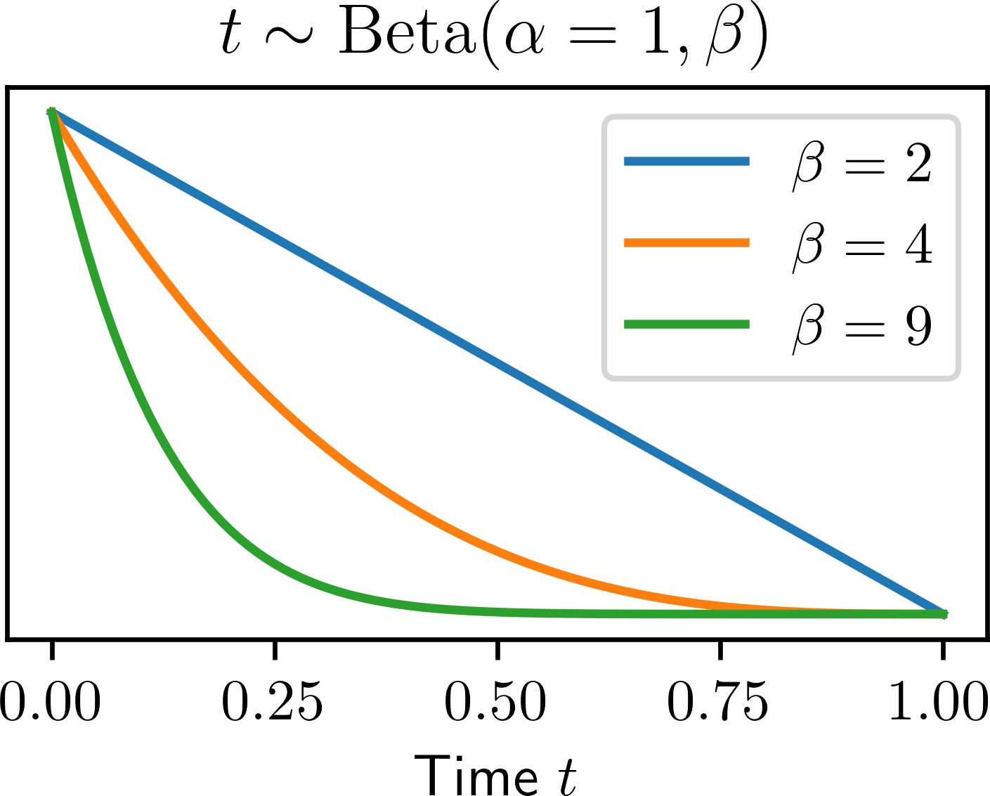
Figure 5: Temperature distributions.

Minibatching

During training we assign randomly each image $\mathbf{x}_{n}$ in each minibatch to either noising, burring or clean role. For the noisy and blurry images we further sample separate temperatures $t_{n}\sim\mathrm{Beta}(\alpha,\beta)$ from a Beta distribution per image. We choose by default $\alpha=1$ and $\beta=2$, which results in average temperature $\mathbb{E}[t]=1/3$.

Training

We use a preact-ResNet-50 (He et al., 2016) with $23.7$ million parameters. We train with SGD using learning rate of $0.01$ for 300 epochs, and use a simple Cosine learning rate (Loshchilov and Hutter, 2016). We use minibatches of 128, and cross-entropy loss. Mollification incurs only a minor running time increase similar to other augmentations.

Metrics

We consider error, negative log likelihood $-\log p(\mathbf{y}|\mathbf{f}(\mathbf{x}))$ (NLL), and expected calibration error (ECE) (Guo et al., 2017). We repeat the metrics on corrupted validation images from CIFAR-10-C, CIFAR-100-C and TinyImageNet-C, which contain $75$ corruptions of each validation image using $15$ types of corruptions at 5 corruption magnitude levels (Hendrycks and Dietterich, 2019). The corruptions divide in four categories of noise masks (3/15), blurs (4/15), weather effects (3/15), and colorisation or compression artifacts (5/15).

We find that natural augmentations of flips (F), crops (C) and rotations (R) are always necessary to train CNNs to satisfying performance, even with mollification.

4.2 Benchmark results

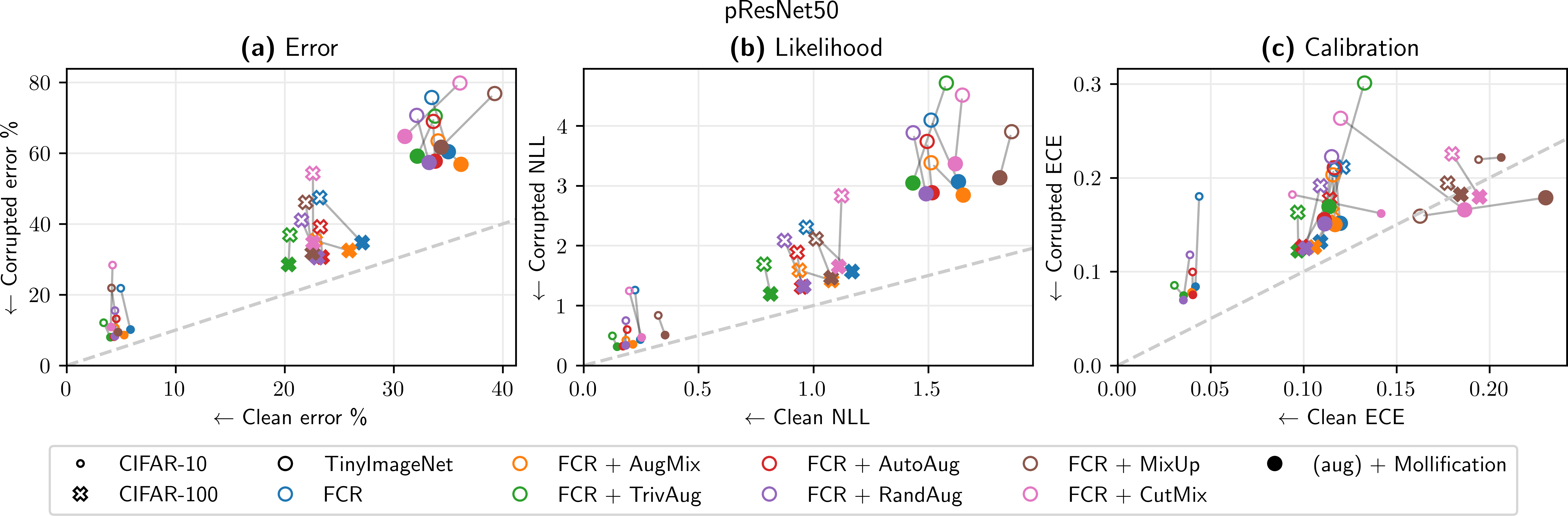
Figure 6: Adding mollification ( $\cdots$ ) to augmentations ( $\cdots$ ) improves corrupted accuracy (a), likelihood (b) and calibration (c) over CIFAR-10, CIFAR-100 and TinyImageNet.

We report benchmark results on Table 1. We first observe that amongst the classic augmentation techniques TrivAug combined with FCR is superior with errors of 3.4%, 20.5% and 33.8% in CIFAR-10, CIFAR-100 and TinyImageNet, respectively. Notably, we struggled to achieve good performance with MixUp and CutMix.

When we include mollification, we again observe that TrivAug+Mollification yields highest performance, while mollification improves corrupted image errors on all 6 augmentations on all datasets. On CIFAR-10 we improve corrupted error $12.1\%\rightarrow 8.0\%$, on CIFAR-100 $36.9\%\rightarrow 28.5\%$ and on TinyImageNet $70\%\rightarrow 59\%$. Mollification also improves the clean performance on the larger TinyImageNet ($33.8\%\rightarrow 32.2\%$), has little effect on CIFAR-100, and slightly decreases on CIFAR-10. We also observe minor calibration improvements from mollification on clean images, while we observe some 20% to 40% improvements on corrupted calibration.

Fig. 6 shows the relationship between clean and corrupted predictions across the datasets, and indicates that mollification consistenly narrows the gap between clean and corrupted metrics.

4.3 Ablation: How to choose mollification and its intensity?

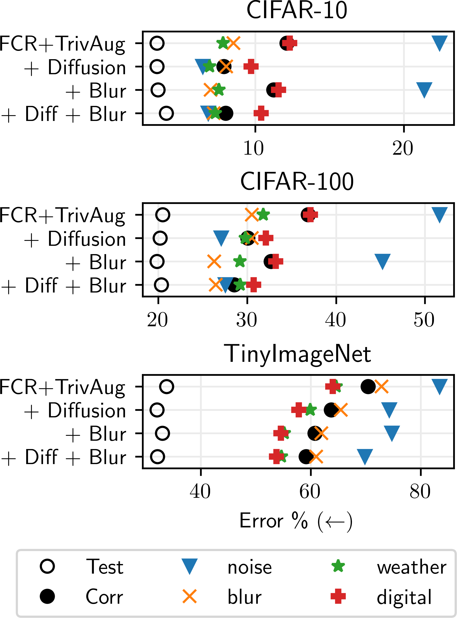
(a)

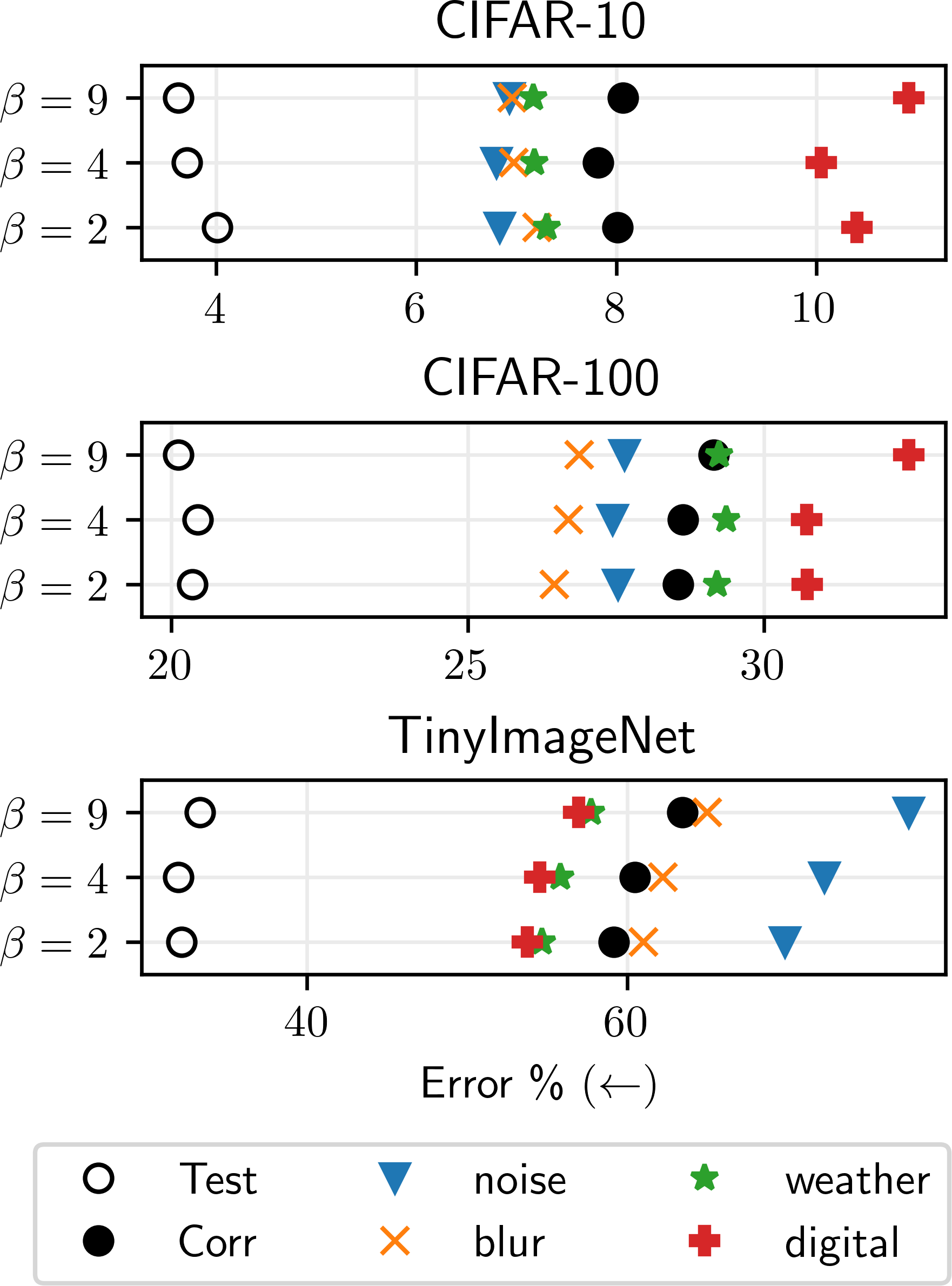
(b)

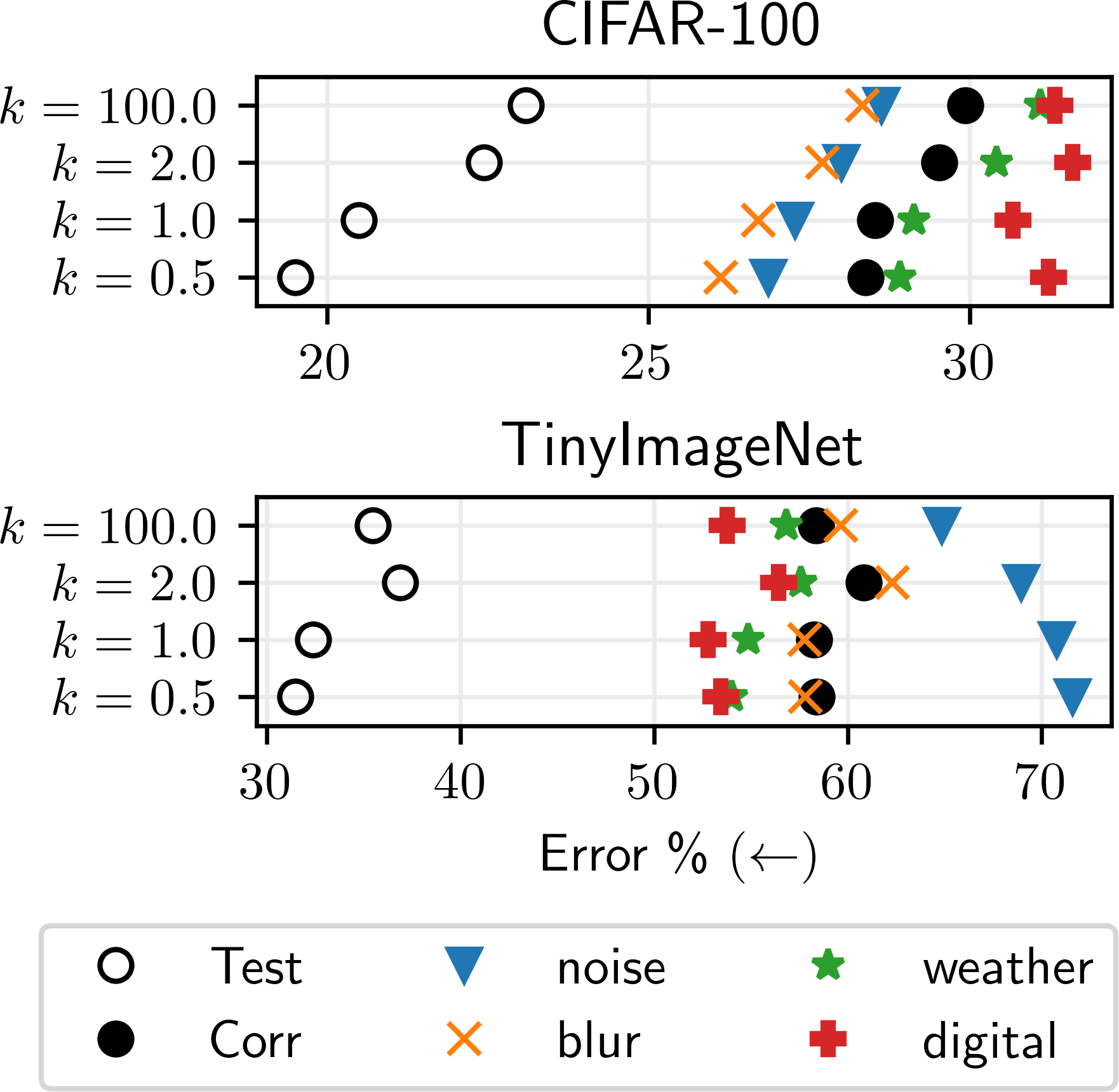
(c)

Figure 7: Combining substantial noising and blurring mollification with greedy label smoothing yields good results.

Next, we consider the mollification mode, and its hyperparameters. Fig. 7(a) shows that on smaller CIFAR images noise diffusion improves more than blurring, while on larger TinyImageNet blurring is more advantageous (see Fig. 8). Combining both modes during training is superior in all cases. Notably, training under blur also improves robustness to test noising on TinyImageNet. We also observe that mollification gives highest performance improvements to ‘weather’ and ‘digital’ test corruptions, despite not encoding for them during training time.

Fig. 7(b) shows that relatively large mollification amounts with $\beta=2$ gives the best performance, while panel Fig. 7(b) shows benefits of more aggressive label decay with $k\leq 1$.

Figure 8: Blurring mollification improves error against all corruption types evenly, while incorporating noising mollification adds slight benefits. Polygon size indicates corruption severity from triangles (1) to heptagons (5), experiment on TinyImageNet.

4.4 Effect of corruption severity

We visualise the performance w.r.t. corruption severity in Fig. 9 for the FCR + TrivAug base augmentation. The results show a consistent pattern of more drastic corruptions being more difficult to predict. The mollified versions are in almost all cases better than the corresponding non-mollified ones on all corruption intensities, while giving similar performance on clean images (zero severity).

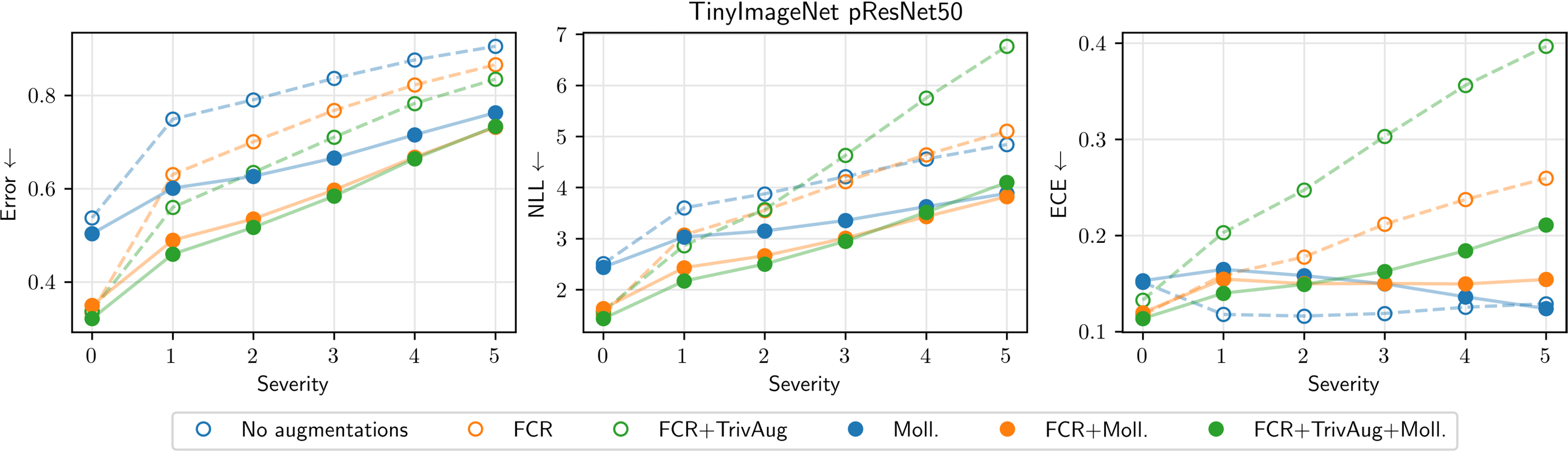
Figure 9: Adding mollification improves augmented models over the corruption severity.

4.5 Which corruptions do we improve?

Table 2: Breakdown of errors over individual corruption types CIFAR-10, CIFAR-100 and TinyImageNet of a pResNet-50 network.

			noise			blur				weather				digital
		Clean	shot	impulse	gauss	motion	zoom	defocus	glass	fog	frost	snow	bright	jpg	pixel	elastic	contrast	mean
CIFAR10	FCR+TrivAug	3.4	23	13	31	10.0	6.2	5.5	12	6.3	12	9.3	3.9	16	21	7.4	4.4	12
	+ Diffusion	3.4	5.7	7.3	6.4	9.4	6.6	5.8	10	6.8	8.4	8.6	4.0	12	15	7.2	4.9	7.6
	+ Blur	3.5	20	17	27	8.1	4.8	4.1	11	6.4	11	9.2	4.0	17	18	6.5	4.7	11
	+ Diff+Blur	4.0	6.2	7.5	6.8	8.8	5.0	4.6	10	7.1	8.5	9.1	4.5	14	16	6.7	5.3	7.8
CIFAR100	FCR+TrivAug	20	54	39	63	32	28	25	38	30	41	33	23	47	47	30	25	36
	+ Diffusion	20	25	30	26	32	29	27	34	31	34	32	23	37	36	29	26	29
	+ Blur	20	45	40	51	28	23	21	33	29	36	31	22	46	36	26	25	32
	+ Diff+Blur	20	25	31	26	28	23	22	32	30	33	31	23	39	32	27	25	28
TIN	FCR+TrivAug	34	81	85	85	68	71	76	76	65	65	69	60	59	61	61	76	68
	+ Diffusion	32	70	78	75	61	62	68	70	61	60	64	55	52	55	53	71	62
	+ Blur	33	71	77	77	57	58	64	68	56	56	60	50	51	49	49	69	59
	+ Diff+Blur	32	65	73	71	57	57	63	67	56	54	59	50	50	49	49	68	57

The corruptions in the -C datasets fall into four categories. Fig. 7 shows a general trend of the network being most robust against ‘digital’ and ‘weather’ corruptions, while ‘blur’ corruptions are moderately difficult, and ‘noise’ corruptions are most difficult to predict correctly. Table 2 shows the performance wrt the 15 individual corruptions over the three datasets. Mollification improves consistently: in TinyImageNet all individual corruption types improve between 9 and 16 percentage points from TrivAug, which is the best performing conventional augmentation method.

5 Discussion and conclusion

From the methodological perspective, there are two aspects which we hoped we could improve on. One is the treatment of the augmented likelihood in (2), which we lower bound through Jensen inequality, similarly to Wenzel et al. (2020); a proper treatment of the log-expectation is possible by carrying out a Monte Carlo approximation of the expectation inside the logarithm, correcting it using ideas from Durbin and Koopman (1997) (see Appendix C).

Another aspect is the formulation of a proper likelihood for individual data points, which we currently derive from the cross-entropy loss (Eq. 10); we were able to derive a normalization of the improper likelihood associated with the cross-entropy loss when labels are continuous with domain in $[0,1]$ (see Appendix B). Surprisingly, and disappointingly, none of these ways to recover a proper treatment of the likelihood led to improvements, while complicating the implementation and the numerical stability of the training.

In this work, we present mollification for supervised image recognition by coupling image noising and label smoothing processes for robustness against test-time corruptions. Our work promotes likelihoods that integrate over the space of augmentations, and draws connections between generative diffusion models and augmentations. An interesting future work lies in class-specific noising structures, as well as on analysing adversarial robustness. Another future research line is to formally connect diffusion with regularization.

Appendix A Additional results

A.1 Mollification vs severity

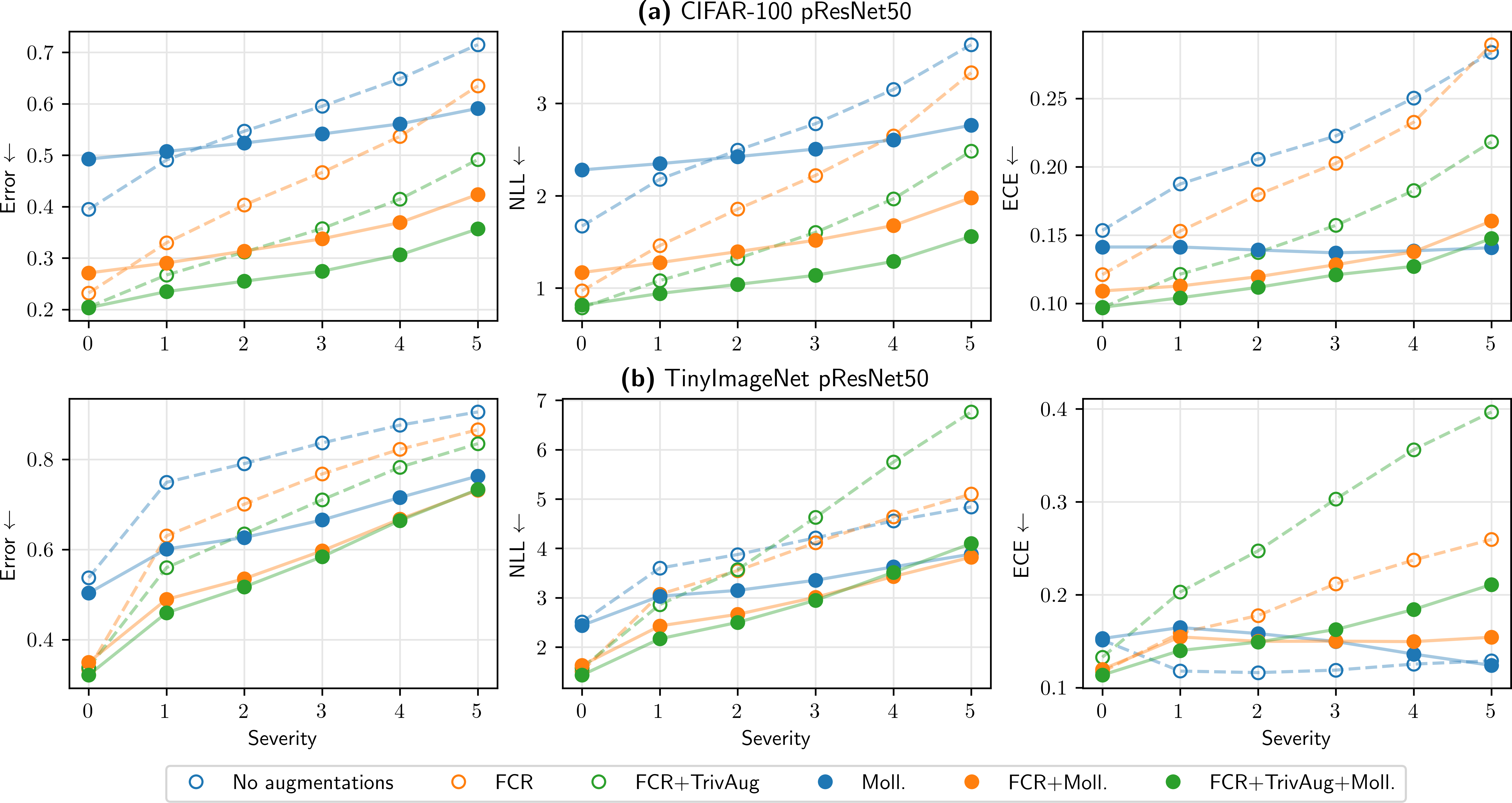
Figure 10: Adding mollification improves augmented models over the corruption severity.

A.2 Result table with standard deviations

Table 3: Results on preactResNet-50 ($23.7$M params.). FCR: horizontal flips, crops and rotations. Standard deviations shown in parentheses.

		CIFAR-10						CIFAR-100						TinyImageNet
		Error $(\downarrow)$		NLL $(\downarrow)$		ECE $(\downarrow)$		Error		NLL		ECE		Error		NLL		ECE
Augmentation	Moll.	clean	corr	clean	corr	clean	corr	clean	corr	clean	corr	clean	corr	clean	corr	clean	corr	clean	corr
presnet50	✗	11.7	29.4	0.49	1.34	0.09	0.22	39.2	60.3	1.64	2.89	0.16	0.24	57.3	84.6	2.73	4.30	0.16	0.11
		(0.10)	(0.63)	(0.01)	(0.04)	(0.00)	(0.01)	(0.40)	(0.39)	(0.02)	(0.06)	(0.01)	(0.01)	(2.12)	(0.33)	(0.13)	(0.02)	(0.01)	(0.00)
FCR	✗	4.9	21.2	0.22	1.14	0.04	0.17	23.2	47.1	0.99	2.32	0.12	0.21	33.9	76.0	1.53	4.11	0.12	0.21
		(0.05)	(1.01)	(0.00)	(0.15)	(0.00)	(0.01)	(0.19)	(0.33)	(0.01)	(0.06)	(0.00)	(0.01)	(0.31)	(0.16)	(0.01)	(0.02)	(0.00)	(0.00)
FCR+RandAug	✗	4.2	15.2	0.18	0.73	0.04	0.12	21.4	41.4	0.87	2.09	0.11	0.19	32.4	70.4	1.45	3.88	0.12	0.22
		(0.15)	(0.41)	(0.00)	(0.03)	(0.00)	(0.00)	(0.15)	(0.59)	(0.00)	(0.07)	(0.00)	(0.00)	(0.15)	(0.20)	(0.01)	(0.04)	(0.00)	(0.00)
FCR+AutoAug	✗	4.6	13.3	0.19	0.60	0.04	0.10	22.7	38.8	0.91	1.86	0.11	0.17	33.8	69.5	1.48	3.77	0.11	0.21
		(0.07)	(0.47)	(0.00)	(0.04)	(0.00)	(0.00)	(0.33)	(0.36)	(0.01)	(0.05)	(0.00)	(0.00)	(0.29)	(0.24)	(0.01)	(0.05)	(0.00)	(0.00)
FCR+AugMix	✗	4.4	10.7	0.18	0.43	0.04	0.08	23.0	35.5	0.94	1.60	0.12	0.16	34.0	63.5	1.52	3.37	0.11	0.20
		(0.06)	(0.26)	(0.00)	(0.01)	(0.00)	(0.00)	(0.31)	(0.34)	(0.02)	(0.02)	(0.00)	(0.00)	(0.28)	(0.18)	(0.01)	(0.03)	(0.00)	(0.01)
FCR+TrivAug	✗	3.4	12.2	0.12	0.50	0.03	0.09	20.2	36.8	0.78	1.69	0.10	0.16	33.8	69.9	1.57	4.64	0.13	0.30
		(0.02)	(0.37)	(0.00)	(0.02)	(0.00)	(0.00)	(0.17)	(0.50)	(0.01)	(0.05)	(0.00)	(0.00)	(0.13)	(0.35)	(0.01)	(0.12)	(0.00)	(0.00)
FCR+MixUp	✗	3.8	21.9	0.29	0.83	0.17	0.20	21.3	45.1	0.96	2.06	0.15	0.18	33.3	72.5	1.75	3.67	0.22	0.15
		(0.17)	(1.47)	(0.02)	(0.04)	(0.01)	(0.02)	(0.49)	(0.72)	(0.04)	(0.06)	(0.02)	(0.03)	(0.36)	(0.35)	(0.04)	(0.03)	(0.01)	(0.01)
FCR+CutMix	✗	3.9	28.2	0.22	1.19	0.11	0.19	22.6	54.3	1.12	2.81	0.18	0.22	31.7	76.4	1.52	4.05	0.13	0.18
		(0.17)	(0.73)	(0.01)	(0.11)	(0.01)	(0.02)	(0.05)	(0.36)	(0.00)	(0.11)	(0.01)	(0.02)	(0.27)	(0.21)	(0.02)	(0.04)	(0.00)	(0.01)
presnet50	✓	15.3	20.6	0.65	0.83	0.11	0.13	49.5	54.7	2.29	2.54	0.15	0.14	50.1	67.3	2.42	3.39	0.15	0.14
		(0.07)	(0.21)	(0.01)	(0.01)	(0.00)	(0.00)	(0.20)	(0.17)	(0.01)	(0.01)	(0.00)	(0.00)	(0.18)	(0.19)	(0.01)	(0.01)	(0.00)	(0.00)
FCR	✓	5.8	10.2	0.24	0.43	0.04	0.08	27.0	34.7	1.16	1.56	0.11	0.13	35.3	60.1	1.63	3.04	0.12	0.15
		(0.17)	(0.15)	(0.01)	(0.01)	(0.00)	(0.00)	(0.07)	(0.19)	(0.01)	(0.01)	(0.00)	(0.00)	(0.07)	(0.20)	(0.01)	(0.02)	(0.00)	(0.01)
FCR+RandAug	✓	4.4	8.3	0.18	0.34	0.04	0.07	23.2	30.6	0.96	1.33	0.10	0.13	33.5	57.2	1.51	2.85	0.11	0.15
		(0.06)	(0.10)	(0.00)	(0.01)	(0.00)	(0.00)	(0.07)	(0.18)	(0.00)	(0.01)	(0.00)	(0.00)	(0.27)	(0.16)	(0.01)	(0.01)	(0.00)	(0.00)
FCR+AutoAug	✓	4.2	8.2	0.17	0.33	0.04	0.07	23.7	30.8	0.96	1.32	0.10	0.13	34.1	58.0	1.52	2.90	0.11	0.15
		(0.05)	(0.15)	(0.00)	(0.01)	(0.00)	(0.00)	(0.12)	(0.24)	(0.00)	(0.01)	(0.00)	(0.00)	(0.06)	(0.27)	(0.01)	(0.03)	(0.00)	(0.00)
FCR+AugMix	✓	5.4	8.7	0.22	0.36	0.04	0.08	25.7	32.3	1.09	1.42	0.10	0.13	36.0	57.1	1.66	2.84	0.12	0.15
		(0.11)	(0.11)	(0.00)	(0.01)	(0.00)	(0.00)	(0.30)	(0.11)	(0.01)	(0.00)	(0.00)	(0.00)	(0.27)	(0.19)	(0.01)	(0.01)	(0.00)	(0.00)
FCR+TrivAug	✓	3.7	7.7	0.14	0.30	0.03	0.07	20.5	28.4	0.81	1.19	0.09	0.12	32.4	59.2	1.43	3.04	0.11	0.17
		(0.07)	(0.33)	(0.00)	(0.02)	(0.00)	(0.00)	(0.20)	(0.35)	(0.01)	(0.02)	(0.00)	(0.00)	(0.21)	(0.62)	(0.01)	(0.05)	(0.00)	(0.00)
FCR+MixUp	✓	4.5	9.4	0.34	0.50	0.20	0.21	23.3	32.3	1.12	1.51	0.20	0.20	34.3	61.9	1.81	3.15	0.23	0.18
		(0.10)	(0.22)	(0.01)	(0.01)	(0.01)	(0.00)	(0.38)	(0.30)	(0.03)	(0.01)	(0.01)	(0.00)	(0.29)	(0.25)	(0.02)	(0.03)	(0.00)	(0.01)
FCR+CutMix	✓	4.0	10.7	0.26	0.48	0.15	0.17	22.5	34.7	1.13	1.66	0.21	0.19	31.2	65.0	1.65	3.39	0.20	0.17
		(0.06)	(0.24)	(0.01)	(0.01)	(0.00)	(0.00)	(0.06)	(0.20)	(0.03)	(0.02)	(0.02)	(0.01)	(0.34)	(0.20)	(0.03)	(0.01)	(0.01)	(0.00)

Appendix B Derivation of the Normalization Constant for the Label Smoothing Likelihood

Let’s consider label smoothing with soft labels defined as

$$\mathbf{y}^{\mathrm{LS}}=(1-a)\mathbf{y}^{\mathrm{onehot}}+\frac{a}{C}\mathbf{1},$$

where, compared to Eq. 6 we have introduced $a=\gamma_{t}-1$.

We are interested in deriving an expression for a proper cross-entropy-based likelihood function expressing $p(\mathbf{y}^{\mathrm{LS}}|\mathbf{x};\theta)$. In other words, we require that $p(\mathbf{y}^{\mathrm{LS}}|\mathbf{x};\theta)$ is indeed a proper distribution over $\mathbf{y}^{\mathrm{LS}}$. The difficulty is that the domain of the labels is now continuous and the cross-entropy loss does not correspond to the negative of the logarithm of a properly normalized likelihood.

Soft labels $\mathbf{y}^{\mathrm{LS}}$ depend on $a$ and $\mathbf{y}^{\mathrm{onehot}}$. For simplicity, let’s denote the one-hot vectors $\mathbf{y}^{\mathrm{onehot}}$ with a one in position $j$ as $\mathbf{e}_{j}$. With this definition, the normalization constant to obtain a proper likelihood can be expressed as follows:

$$Z=\sum_{j=1}^{C}\int_{0}^{1}\prod_{i=1}^{C}f_{i}^{(\mathbf{y}^{\mathrm{LS}}(a,\mathbf{e}_{j}))_{i}}da$$

Note that $f_{i}$ here represent probabilities of class label $i$, that is these are the values post-softmax transformation of the output of the network. Without loss of generality, let’s focus on the case $j=1$:

$$\int_{0}^{1}\prod_{i=1}^{C}f_{i}^{(\mathbf{y}^{\mathrm{LS}}(a,\mathbf{e}_{1}))_{i}}da=\int_{0}^{1}f_{1}^{1-a+\frac{a}{C}}f_{2}^{\frac{a}{C}}\ldots f_{C}^{\frac{a}{C}}da$$

which we can simplify into:

$$f_{1}\int_{0}^{1}f_{1}^{a\frac{1-C}{C}}f_{2}^{\frac{a}{C}}\ldots f_{C}^{\frac{a}{C}}da=f_{1}\int_{0}^{1}\left(f_{1}^{\frac{1-C}{C}}f_{2}^{\frac{1}{C}}\ldots f_{C}^{\frac{1}{C}}\right)^{a}da$$

We can proceed in a similar way for any $\mathbf{e}_{j}$, and we can compact the expression of the integral further as

$$f_{j}\int_{0}^{1}\left(f_{j}^{-1}\prod_{i=1}^{C}f_{i}^{\frac{1}{C}}\right)^{a}da=f_{j}\int_{0}^{1}\left(\frac{K}{f_{j}}\right)^{a}da$$

where we have introduced $K=\prod_{i=1}^{C}f_{i}^{\frac{1}{C}}$

So finally the normalization constant $Z$ is the sum over $j$ of these integrals, for which the solution is in the form:

$$\int_{0}^{1}z^{a}da=\frac{z-1}{\log z}$$

thus obtaining

$$Z=\sum_{j=1}^{C}f_{j}\int_{0}^{1}\left(\frac{K}{f_{j}}\right)^{a}da=\sum_{j=1}^{C}\frac{K-f_{j}}{\log(K)-\log(f_{j})}$$

Appendix C Inference of the Augmented Likelihood

The augmented likelihood (2) is intractable due to an integral over the space of continuous corruptions or augmentations. Furthermore, simple Monte-Carlo averaging of the likelihood is biased for $K>1$ (Durbin and Koopman, 1997),

$$\log p(\mathcal{D}|\theta) =\sum_{n=1}^{N}\log\int p(\mathbf{y}_{n}|\mathbf{x}_{n},\phi;\theta)p(\phi)d\phi.$$ (14)

$$\approx\sum_{n=1}^{N}\log\frac{1}{K}\sum_{k=1}^{K}p(\mathbf{y}_{n}|\mathbf{x}_{n},\phi_{k};\theta),$$ (15)

where $\phi_{k}\sim p(\phi)$. In practise the MC under-estimates the likelihood.

Lower bound on log expectation

The intractable likelihood can be approximated in multiple ways. We can simply estimate the biased Jensen posterior by moving the log inside the integral (Wenzel et al., 2020),

$$\log p(\mathcal{D}|\theta) =\sum_{n=1}^{N}\log\int p(\mathbf{y}_{n}|\mathbf{x}_{n},\phi;\theta)p(\phi)d\phi.$$ (16)

$$\geq\sum_{n=1}^{N}\int\log p(\mathbf{y}_{n}|\mathbf{x}_{n},\phi_{k};\theta)p(\phi)d\phi$$ (17)

$$\approx\sum_{n=1}^{N}\frac{1}{K}\sum_{k=1}^{K}\log p(\mathbf{y}_{n}|\mathbf{x}_{n},\phi_{k};\theta),$$ (18)

where $\phi_{k}\sim p(\phi)$. This represents a lower bound of the true augmented likelihood, for which Monte-Carlo approximation is unbiased. The Jensen bound can be applied with importance sampling to tighten the bound (Burda et al., 2016; Luo et al., 2020).

Bias correction

We can also apply a bias-correction (Durbin and Koopman, 1997; Shephard and Pitt, 1997) to the non-log sample mean. First, we consider Monte-Carlo approximation of an integral whose logarithm we wish to evaluate,

$$I =\int p(\mathbf{y}|\mathbf{x},\phi,\theta)p(\phi)d\phi$$ (19)

$$I \approx I_{K}=\frac{1}{K}\sum_{k}p(\mathbf{y}|\phi_{k},\mathbf{x},\theta),\quad\phi_{k}\sim p(\phi).$$ (20)

It can be shown that the estimator $I_{K}$ can be unbiased (Durbin and Koopman, 1997; Shephard and Pitt, 1997)

$$\log I \approx\log I_{K}+\frac{1}{2}\frac{\operatorname{var}[I_{K}]}{I_{K}^{2}}$$ (21)

$$\operatorname{var}[I_{K}] =\frac{1}{K(K-1)}\sum_{k}(p(\mathbf{y}|\mathbf{x},\phi_{k},\theta)-I_{K})^{2}$$ (22)

$$0 =\mathbb{E}\left[\log I_{K}+\frac{1}{2}\frac{\operatorname{var}[I_{K}]}{I_{K}^{2}}\right].$$ (23)

The correction makes the log-integral unbiased wrt different samplings $(\phi_{1},\ldots,\phi_{K})\sim p(\phi)$. With $K=1$ naive approximation the log-integral is already unbiased, but suffers from large variance. In image classification, $K$ refers to the number of corruptions per image within a mini-batch. The correction is the most beneficial in small-$K$ regimes. For instance, in Batch Augmentation multiple instances of each image are used within a batch (Hoffer et al., 2020).

Tempering vs augmented likelihood

Our additive augmented likelihood (2) aligns with the ‘Jensen’ likelihoods discussed by Wenzel et al. (2020). In contrast, Kapoor et al. (2022) argues for multiplicative tempered augmented likelihood

$$p_{\mathrm{geom}}(\mathcal{D}|\theta) =\prod_{n=1}^{N}\prod_{k=1}^{K}p\big{(}\mathbf{y}_{n}|\mathbf{x}_{n},\phi,\theta\big{)}^{1/K},$$ (24)

where the augmentations are aggregated by a geometric mean. These approaches are connected: the geometric likelihood (24) is the lower bound (17) of the augmented likelihood (16). In the geometric likelihood we can interpret the augmentations as down-weighted data points, which are assumed to factorize despite not being i.i.d.. In augmented likelihood we interpret the data points as i.i.d. samples, and augmentations as expanding each sample into a distribution, which leads to a product over observations and integral over augmentations.

References

- Bachmann et al. (2022) G. Bachmann, L. Noci, and T. Hofmann. How tempering fixes data augmentation in Bayesian neural networks. In ICML, 2022.
- Bansal et al. (2024) A. Bansal, E. Borgnia, H.-M. Chu, J. Li, H. Kazemi, F. Huang, M. Goldblum, J. Geiping, and T. Goldstein. Cold diffusion: Inverting arbitrary image transforms without noise. Advances in Neural Information Processing Systems, 36, 2024.
- Burda et al. (2016) Y. Burda, R. Grosse, and R. Salakhutdinov. Importance weighted autoencoders. In ICLR, 2016.
- Cifarelli and Regazzini (1996) D. M. Cifarelli and E. Regazzini. De Finetti’s contribution to probability and statistics. Statistical Science, 11(4):253–282, 1996.
- Cubuk et al. (2019) E. D. Cubuk, B. Zoph, D. Mané, V. Vasudevan, and Q. V. Le. AutoAugment: Learning augmentation strategies from data. In CVPR, 2019.
- DeVries and Taylor (2017) T. DeVries and G. W. Taylor. Improved regularization of convolutional neural networks with cutout. arXiv, 2017.
- Dosovitskiy et al. (2021) A. Dosovitskiy, L. Beyer, A. Kolesnikov, D. Weissenborn, X. Zhai, T. Unterthiner, M. Dehghani, M. Minderer, G. Heigold, S. Gelly, et al. An image is worth 16x16 words: Transformers for image recognition at scale. In ICLR, 2021.
- Durbin and Koopman (1997) J. Durbin and S. Koopman. Monte Carlo maximum likelihood estimation for non-Gaussian state space models. Biometrika, 1997.
- Fong et al. (2023) E. Fong, C. Holmes, and S. G. Walker. Martingale posterior distributions. Journal of the Royal Statistical Society Series B: Statistical Methodology, 85(5):1357–1391, 2023.
- Goodfellow et al. (2020) I. Goodfellow, J. Pouget-Abadie, M. Mirza, B. Xu, D. Warde-Farley, S. Ozair, A. Courville, and Y. Bengio. Generative adversarial networks. Communications of the ACM, 2020.
- Guo et al. (2017) C. Guo, G. Pleiss, Y. Sun, and K. Q. Weinberger. On calibration of modern neural networks. In ICML, 2017.
- He et al. (2016) K. He, X. Zhang, S. Ren, and J. Sun. Identity mappings in deep residual networks. In ECCV, 2016.
- Hendrycks and Dietterich (2019) D. Hendrycks and T. Dietterich. Benchmarking neural network robustness to common corruptions and perturbations. In ICLR, 2019.
- Hendrycks et al. (2020) D. Hendrycks, N. Mu, E. D. Cubuk, B. Zoph, J. Gilmer, and B. Lakshminarayanan. Augmix: A simple data processing method to improve robustness and uncertainty. In ICLR, 2020.
- Hendrycks et al. (2022) D. Hendrycks, A. Zou, M. Mazeika, L. Tang, B. Li, D. Song, and J. Steinhardt. PixMix: Dreamlike pictures comprehensively improve safety measures. In CVPR, 2022.
- Ho and Salimans (2021) J. Ho and T. Salimans. Classifier-free diffusion guidance. In NeurIPS workshop on Deep Generative Models, 2021.
- Ho et al. (2020) J. Ho, A. Jain, and P. Abbeel. Denoising diffusion probabilistic models. In NeurIPS, 2020.
- Hoffer et al. (2020) E. Hoffer, T. Ben-Nun, I. Hubara, N. Giladi, T. Hoefler, and D. Soudry. Augment your batch: Improving generalization through instance repetition. In CVPR, 2020.
- Hoogeboom and Salimans (2023) E. Hoogeboom and T. Salimans. Blurring diffusion models. In ICLR, 2023.
- Izmailov et al. (2021) P. Izmailov, S. Vikram, M. D. Hoffman, and A. G. Wilson. What are bayesian neural network posteriors really like? In ICML, 2021.
- Kapoor et al. (2022) S. Kapoor, W. Maddox, P. Izmailov, and A. G. Wilson. On uncertainty, tempering, and data augmentation in bayesian classification. In NeurIPS, 2022.
- Karras et al. (2018) T. Karras, T. Aila, S. Laine, and J. Lehtinen. Progressive growing of GANs for improved quality, stability, and variation. In ICLR, 2018.
- Kingma et al. (2021) D. Kingma, T. Salimans, B. Poole, and J. Ho. Variational diffusion models. In NeurIPS, 2021.
- Kingma and Welling (2014) D. P. Kingma and M. Welling. Auto-encoding variational bayes. In ICLR, 2014.
- Kirichenko et al. (2023) P. Kirichenko, M. Ibrahim, R. Balestriero, D. Bouchacourt, R. Vedantam, H. Firooz, and A. G. Wilson. Understanding the detrimental class-level effects of data augmentation. In NeurIPS, 2023.
- Krizhevsky (2009) A. Krizhevsky. Learning multiple layers of features from tiny images. Technical report, 2009.
- Le and Yang (2015) Y. Le and X. S. Yang. Tiny ImageNet visual recognition challenge. 2015.
- Li et al. (2023) A. C. Li, M. Prabhudesai, S. Duggal, E. Brown, and D. Pathak. Your diffusion model is secretly a zero-shot classifier. In ICCV, 2023.
- Li et al. (2020) W. Li, G. Dasarathy, and V. Berisha. Regularization via structural label smoothing. In AISTATS, 2020.
- Lienen and Hüllermeier (2021) J. Lienen and E. Hüllermeier. From label smoothing to label relaxation. In AAAI, 2021.
- Loshchilov and Hutter (2016) I. Loshchilov and F. Hutter. Sgdr: Stochastic gradient descent with warm restarts. In ICLR, 2016.
- Luo et al. (2020) Y. Luo, A. Beatson, M. Norouzi, J. Zhu, D. Duvenaud, R. P. Adams, and R. T. Chen. Sumo: Unbiased estimation of log marginal probability for latent variable models. In ICLR, 2020.
- Maher and Kull (2021) M. Maher and M. Kull. Instance-based label smoothing for better calibrated classification networks. In ICMLA, 2021.
- Müller et al. (2019) R. Müller, S. Kornblith, and G. E. Hinton. When does label smoothing help? In NeurIPS, 2019.
- Müller and Hutter (2021) S. G. Müller and F. Hutter. Trivialaugment: Tuning-free yet state-of-the-art data augmentation. In ICCV, 2021.
- Nabarro et al. (2022) S. Nabarro, S. Ganev, A. Garriga-Alonso, V. Fortuin, M. van der Wilk, and L. Aitchison. Data augmentation in bayesian neural networks and the cold posterior effect. In UAI, 2022.
- Nichol and Dhariwal (2021) A. Nichol and P. Dhariwal. Improved denoising diffusion probabilistic models. In ICML, 2021.
- Papamakarios et al. (2021) G. Papamakarios, E. Nalisnick, D. J. Rezende, S. Mohamed, and B. Lakshminarayanan. Normalizing flows for probabilistic modeling and inference. JMLR, 2021.
- Qin et al. (2023) Y. Qin, X. Wang, B. Lakshminarayanan, E. H. Chi, and A. Beutel. What are effective labels for augmented data? improving calibration and robustness with AutoLabel. In IEEE Conference on Secure and Trustworthy Machine Learning, 2023.
- Radford et al. (2021) A. Radford, J. W. Kim, C. Hallacy, A. Ramesh, G. Goh, S. Agarwal, G. Sastry, A. Askell, P. Mishkin, J. Clark, et al. Learning transferable visual models from natural language supervision. In ICML, 2021.
- Rissanen et al. (2023) S. Rissanen, M. Heinonen, and A. Solin. Generative modelling with inverse heat dissipation. In ICLR, 2023.
- Ross (1980) S. M. Ross. Introduction to probability models. Academic press, 1980.
- Sensoy et al. (2018) M. Sensoy, L. Kaplan, and M. Kandemir. Evidential deep learning to quantify classification uncertainty. In NeurIPS, 2018.
- Shephard and Pitt (1997) N. Shephard and M. Pitt. Likelihood analysis of non-gaussian measurement time series. Biometrika, 1997.
- Song et al. (2021) Y. Song, J. Sohl-Dickstein, D. P. Kingma, A. Kumar, S. Ermon, and B. Poole. Score-based generative modeling through stochastic differential equations. In ICLR, 2021.
- Szegedy et al. (2016) C. Szegedy, V. Vanhoucke, S. Ioffe, J. Shlens, and Z. Wojna. Rethinking the inception architecture for computer vision. In CVPR, 2016.
- Teney et al. (2024) D. Teney, J. Wang, and E. Abbasnejad. Selective mixup helps with distribution shifts, but not (only) because of mixup. In ICML, 2024.
- Thulasidasan et al. (2019) S. Thulasidasan, G. Chennupati, J. A. Bilmes, T. Bhattacharya, and S. Michalak. On mixup training: Improved calibration and predictive uncertainty for deep neural networks. In NeurIPS, 2019.
- Tran et al. (2023) B.-H. Tran, G. Franzese, P. Michiardi, and M. Filippone. One-line-of-code data mollification improves optimization of likelihood-based generative models. In NeurIPS, 2023.
- Vryniotis (2021) V. Vryniotis. How to Train State-Of-The-Art Models Using TorchVision’s Latest Primitives. pytorch.org, 2021.
- Wang et al. (2023) Y. Wang, N. Polson, and V. O. Sokolov. Data Augmentation for Bayesian Deep Learning. Bayesian Analysis, 2023.
- Wenzel et al. (2020) F. Wenzel, K. Roth, B. Veeling, J. Swiatkowski, L. Tran, S. Mandt, J. Snoek, T. Salimans, R. Jenatton, and S. Nowozin. How good is the Bayes posterior in deep neural networks really? In ICML, 2020.
- Wightman et al. (2021) R. Wightman, H. Touvron, and H. Jégou. Resnet strikes back: An improved training procedure in timm. In NeurIPS workshop on ImageNet PPF, 2021.
- Wu and A Williamson (2024) L. Wu and S. A Williamson. Posterior uncertainty quantification in neural networks using data augmentation. In AISTATS, 2024.
- Yao et al. (2022) H. Yao, Y. Wang, S. Li, L. Zhang, W. Liang, J. Zou, and C. Finn. Improving out-of-distribution robustness via selective augmentation. In ICML, 2022.
- Yun et al. (2019) S. Yun, D. Han, S. J. Oh, S. Chun, J. Choe, and Y. Yoo. Cutmix: Regularization strategy to train strong classifiers with localizable features. In ICCV, 2019.
- Zagoruyko and Komodakis (2016) S. Zagoruyko and N. Komodakis. Wide residual networks. In BMVC, 2016.
- Zhang et al. (2018) H. Zhang, M. Cisse, Y. N. Dauphin, and D. Lopez-Paz. mixup: Beyond empirical risk minimization. In ICLR, 2018.