Non-splitting Eulerian-Lagrangian WENO schemes for two-dimensional nonlinear convection-diffusion equations

Abstract

In this paper, we develop high-order, conservative, non-splitting Eulerian-Lagrangian (EL) Runge-Kutta (RK) finite volume (FV) weighted essentially non-oscillatory (WENO) schemes for convection-diffusion equations. The proposed EL-RK-FV-WENO scheme defines modified characteristic lines and evolves the solution along them, significantly relaxing the time-step constraint for the convection term. The main algorithm design challenge arises from the complexity of constructing accurate and robust reconstructions on dynamically varying Lagrangian meshes. This reconstruction process is needed for flux evaluations on time-dependent upstream quadrilaterals and time integrations along moving characteristics. To address this, we propose a strategy that utilizes a WENO reconstruction on a fixed Eulerian mesh for spatial reconstruction, and updates intermediate solutions on the Eulerian background mesh for implicit-explicit RK temporal integration. This strategy leverages efficient reconstruction and remapping algorithms to manage the complexities of polynomial reconstructions on time-dependent quadrilaterals, while ensuring local mass conservation. The proposed scheme ensures mass conservation due to the flux-form semi-discretization and the mass-conservative reconstruction on both background and upstream cells. Extensive numerical tests have been performed to verify the effectiveness of the proposed scheme.

65M25, 65M60, 76M10

1 Introduction

Simulating convection-diffusion phenomena has a wide range of applications, including fluid dynamics [36, 21, 10], materials science [30, 33, 7], and geophysics [29, 28]. In this paper, we consider a scalar convection-diffusion equation:

(1) $$u_{t}+\nabla_{\mathbf{x}}\cdot(\mathbf{F}(u,\mathbf{x},t))=\epsilon\Delta u,$$

where $\epsilon\geq 0$. Existing methods include the Eulerian [13, 18] and Lagrangian approaches [11, 3, 4, 5]. The Eulerian approach evolves the equation upon a fixed spatial mesh (or Eulerian mesh), and such methods are usually robust and relatively easy to implement, but they suffer from time-step constraints. The Lagrangian approach follows characteristics in time evolution by generating a Lagrangian mesh that moves with the velocity field, allowing for a larger time-step size compared with Eulerian schemes. However, the moving Lagrangian mesh can be greatly distorted, leading to significant challenges in analysis and implementation. Between the two approaches, there are the Eulerian-Lagrangian (EL) approach [32, 1, 25], the semi-Lagrangian (SL) approach [35, 31, 16], and the arbitrary Lagrangian-Eulerian (ALE) approach [8, 24, 38]. Both the EL and SL approaches utilize a fixed background mesh and accurately or approximately track information propagation along characteristics, which helps them ease the numerical time-step constraint. The schemes from the ALE approach consider a dynamically moving mesh. These approaches aim to balance between the Eulerian and Lagrangian approaches in various ways, tailored for better efficiency of computational algorithms in different settings.

In this paper, we continue our development of the EL Runge-Kutta (RK) schemes [9, 25], but now in a truly multi-dimensional finite volume (FV) fashion for nonlinear convection-diffusion problems. In the finite volume setting, we need to update only one degree of freedom per cell, as opposed to multiple ones, compared with the previous EL-RK discontinuous Garlerkin (DG) scheme [9]. Building upon the EL-RK framework, we introduce a modified velocity field as a first-order approximation of the analytic velocity field, offering triple benefits: firstly, the modified velocity field has straight characteristic lines, leading to upstream cells with straight edges that are easier to approximate than polygons with curved edges; secondly, tracking characteristics approximately allows a greatly relaxed time-stepping constraint compared with Eulerian methods; thirdly, the EL framework offers flexibility in treating nonlinearity, while integrating diffusion terms, thereby presenting a truly multi-dimensional EL finite volume scheme compared to our earlier work in [16, 25].

Yet new challenges arise in reconstructing high-order polynomials on dynamically varying Lagrangian upstream cells; robust and accurate weighted essentially non-oscillatory (WENO) reconstructions on time-dependent upstream polygons can be computationally complex and expensive. Furthermore, performing high-order time integration along moving characteristics brings new complications in algorithm design. Below, we elaborate major computational roadblocks and our proposed strategy in the following two aspects:

• Spatial reconstruction. The EL RK formulation necessitates flux evaluations at the interface of upstream cells; thus, we need to reconstruct piecewise polynomials on upstream quadrilaterals. Performing WENO reconstruction of polynomials on distorted upstream quadrilaterals, e.g., see the red mesh in Figure 2b, can be computationally involved. Further, shapes of these upstream cells differ in every time-step, leading to expensive mesh-dependent local computations. To address such challenges, we propose to (a) perform a robust and efficient WENO reconstruction of piecewise polynomials on the background Eulerian mesh; and (b) leverage a remapping algorithm to compute cell averages on upstream cells from cell averages on the background Eulerian mesh in a mass conservative fashion [20, 37]. Finally, we perform piecewise polynomial reconstruction on upstream quadrilaterals, with preservation of cell averages computed in (b), while utilizing the piecewise polynomials on Eulerian mesh reconstructed in (a) for accuracy consideration.

• Implicit-explicit (IMEX) RK temporal integration along linear approximation of characteristics. A major computational challenge in performing method-of-lines time integrations along moving meshes is the complexity again in polynomial reconstructions of solutions on quadrilateral meshes that are time varying. To address this issue, we propose to update intermediate IMEX solutions at the background Eulerian mesh as in [16, 25], for which efficient reconstruction and the remapping algorithms can be utilized to faciliate the polynomial reconstruction on time-dependent quadrilaterals as mentioned above.

We emphasize that efficient polynomial reconstruction on a fixed Eulerian mesh serves as a cornerstone in our EL-RK algorithm, upon which polynomial reconstructions on distorted upstream quadrilaterals are performed. Indeed, WENO reconstructions on a background Eulerian mesh have been well developed in the literature [23, 17, 39, 14, 37]. In this paper, we further improve upon our previous work [37] and propose a new 2D WENO reconstruction. This new approach strikes a good balance between controlling numerical oscillations and achieving optimal accuracy, by optimizing small stencil polynomial approximations and the weighting strategy.

The rest of the paper is organized as follows. Section 2 presents the proposed EL-RK-FV-WENO schemes; Section 3 presents extensive numerical results showcasing the scheme’s effectiveness. Finally, we conclude in Section 4.

2 EL-RK-FV-WENO schemes

In Section 2.1, we introduce a first-order EL-RK-FV scheme for a linear convection-diffusion equation. Then, building upon the basic concepts introduced in Section 2.1, we discuss the construction of high-order EL-RK-FV-WENO schemes in Section 2.2. Finally, the extension of the proposed EL-RK-FV-WENO scheme to a nonlinear model is presented in Section 2.3.

2.1 First-order EL-RK-FV scheme

Consider

(2) $$u_{t}+(a(x,y,t)u)_{x}+(b(x,y,t)u)_{y}=\epsilon(u_{xx}+u_{yy}).$$

We assume a rectangle computational domain denoted by $\Omega:=[x_{L},x_{R}]\times[y_{B},y_{T}]$ with following partitions for each dimension

$$x_{L}=x_{\frac{1}{2}}<x_{\frac{3}{2}}<\ldots<x_{i-\frac{1}{2}}<x_{i+\frac{1}{2}}<\ldots<x_{N+\frac{1}{2}}=x_{R},$$

$$y_{B}=y_{\frac{1}{2}}<y_{\frac{3}{2}}<\ldots<y_{j-\frac{1}{2}}<y_{j+\frac{1}{2}}<\ldots<y_{N+\frac{1}{2}}=y_{T}$$

with $x_{i}:=(x_{i-\frac{1}{2}}+x_{i+\frac{1}{2}})/2$, $y_{j}:=(y_{j-\frac{1}{2}}+y_{j+\frac{1}{2}})/2$, $\Delta x_{i}=x_{i+\frac{1}{2}}-x_{i-\frac{1}{2}}$, $\Delta y_{j}=y_{j+\frac{1}{2}}-y_{j-\frac{1}{2}}$, $I_{i}^{x}:=[x_{i-\frac{1}{2}},x_{i+\frac{1}{2}}]$, $I_{j}^{y}:=[y_{j-\frac{1}{2}},y_{j+\frac{1}{2}}]$ and $I_{i,j}:=I_{i}^{x}\times I_{j}^{y},\quad\forall i,j$. We define the numerical solutions on the Eulerian mesh as $\{\overline{u}^{n}_{i,j}\}$, which approximate the averages of the $u(x,y,t^{n})$ over the Eulerian cells $\{I_{i,j}\}$, i.e. $\{\frac{1}{|I_{i,j}|}\iint_{I_{i,j}}u(x,y,t^{n})dxdy\}$.

To derive an EL-RK-FV formulation, we first define a modified velocity field $(\alpha(x,y,t),\beta(x,y,t))$. The definition of $(\alpha(x,y,t),\beta(x,y,t))$ is summarized as follows.

1. At $t=t^{n+1}$, $\alpha(x,y,t^{n+1})$ and $\beta(x,y,t^{n+1})$ belong to $Q^{1}(I_{i,j})$ satisfying

   (3) $$\begin{split}\alpha(x_{i\pm\frac{1}{2}},y_{j\pm\frac{1}{2}},t^{n+1})=a(x_{i\pm\frac{1}{2}},y_{j\pm\frac{1}{2}},t^{n+1}),\\ \beta(x_{i\pm\frac{1}{2}},y_{j\pm\frac{1}{2}},t^{n+1})=b(x_{i\pm\frac{1}{2}},y_{j\pm\frac{1}{2}},t^{n+1}).\end{split}$$

2. We define a dynamic region (see Figure 1)

   (4) $$\widetilde{I}_{i,j}(t):=\{(x,y)|(x,y)=(\widetilde{x}(t;(\xi,\eta,t^{n+1})),\widetilde{y}(t;(\xi,\eta,t^{n+1}))),(\xi,\eta)\in I_{i,j}\},$$

   where $(\widetilde{x}(t;(\xi,\eta,t^{n+1})),\widetilde{y}(t;(\xi,\eta,t^{n+1})))$ represents the straight line going through $(\xi,\eta,t^{n+1})$ satisfying

   (5) $$\begin{cases}\widetilde{x}(t;(\xi,\eta,t^{n+1}))=\xi+(t-t^{n+1})\alpha(\xi,\eta,t^{n+1}),\\ \widetilde{y}(t;(\xi,\eta,t^{n+1}))=\eta+(t-t^{n+1})\beta(\xi,\eta,t^{n+1}).\end{cases}$$

   We call (5) a modified characteristic line.

3. For $t\in[t^{n},t^{n+1})$ and $(\widetilde{x}(t;(\xi,\eta,t^{n+1})),\widetilde{y}(t;(\xi,\eta,t^{n+1})))\in\widetilde{I}_{i,j}(t)$,

   (6) $$\begin{cases}\alpha(\widetilde{x}(t;(\xi,\eta,t^{n+1})),\widetilde{y}(t;(\xi,\eta,t^{n+1})))=\alpha(\xi,\eta,t^{n+1}),\\ \beta(\widetilde{x}(t;(\xi,\eta,t^{n+1})),\widetilde{y}(t;(\xi,\eta,t^{n+1})))=\beta(\xi,\eta,t^{n+1}).\end{cases}$$

\begin{overpic}[scale={0.3}]{Figures//schematic_EL}\put(33.0,81.0){$I_{i,j}$} \put(29.0,18.0){$\widetilde{I}_{i,j}(t^{n})$} \put(29.0,49.0){$\widetilde{I}_{i,j}(t)$} \put(84.0,17.0){$t^{n}$} \put(84.0,50.0){$t\in(t^{n},t^{n+1})$} \put(84.0,82.0){$t^{n+1}$} \end{overpic}

Figure 1: Schematic illustration for the dynamic region $\widetilde{I}_{i,j}(t)$.

With the definitions above, we can derive

(7) $$\begin{split}&\frac{d}{dt}\iint_{\widetilde{I}_{i,j}(t)}u(x,y,t)dxdy\\ =&\iint_{\widetilde{I}_{i,j}(t)}u_{t}(x,y,t)dxdy+\int_{\partial\widetilde{I}_{i,j}(t)}(\alpha,\beta)u\cdot\mathbf{n}ds\\ =&\iint_{\widetilde{I}_{i,j}(t)}u_{t}(x,y,t)dxdy+\iint_{\widetilde{I}_{i,j}(t)}\left[(au)_{x}+(bu)_{y}\right]dxdy\\ &-\int_{\partial\widetilde{I}_{i,j}(t)}(a,b)u\cdot\mathbf{n}ds+\int_{\partial\widetilde{I}_{i,j}(t)}(\alpha,\beta)u\cdot\mathbf{n}ds\\ =&-\int_{\partial\widetilde{I}_{i,j}(t)}(a-\alpha,b-\beta)u\cdot\mathbf{n}ds+\epsilon\iint_{\widetilde{I}_{i,j}(t)}\Delta udxdy.\end{split}$$

We define that $\mathbf{F}(u,x,y,t):=((a-\alpha)u,(b-\beta)u)$ and provide the concise EL-FV formulation:

(8) $$\begin{split}\frac{d}{dt}\iint_{\widetilde{I}_{i,j}(t)}u(x,y,t)dxdy&=-\int_{\partial\widetilde{I}_{i,j}(t)}\mathbf{F}(u,x,y,t)\cdot\mathbf{n}ds+\epsilon\iint_{\widetilde{I}_{i,j}(t)}\Delta udxdy\\ &=:\mathcal{F}_{i,j}(u;t)+\mathcal{G}_{i,j}(u;t).\end{split}$$

To evaluate the right-hand side (RHS) of (8), we introduce the following notation for semi-discretization:

(9) $$\frac{d\widetilde{u}_{i,j}(t)}{dt}=\widetilde{\mathcal{F}}_{i,j}(\overline{\mathbf{U}};t)+\widetilde{\mathcal{G}}_{i,j}(\overline{\mathbf{U}};t),$$

where

• the notation $\widetilde{\cdot}$ specifies that the integral value corresponds to the characteristic spatial region $\widetilde{I}_{i,j}(t)$,

• $\widetilde{u}_{i,j}(t)$ approximates $\iint_{\widetilde{I}_{i,j}(t)}u(x,y,t)dxdy$,

• $\widetilde{\mathcal{F}}_{i,j}(\overline{\mathbf{U}};t)$ approximates $\mathcal{F}_{i,j}(u;t)$,

• $\widetilde{\mathcal{G}}_{i,j}(\overline{\mathbf{U}};t)$ approximates $\mathcal{G}_{i,j}(u;t)$,

• $\overline{\mathbf{U}}:=\left(\overline{u}_{i,j}(t)\right)_{NxNy}$ represents the finite volumes such that

  (10) $$\overline{u}_{i,j}(t)\approx\frac{1}{|I_{i,j}|}\iint_{I_{i,j}}u(x,y,t)dxdy.$$

Similar to $\overline{\mathbf{U}}$, we can also represent (9) globally as follows:

(11) $$\frac{d\widetilde{\mathbf{U}}(t)}{dt}=\bm{\widetilde{\mathcal{F}}}(\overline{\mathbf{U}};t)+\bm{\widetilde{\mathcal{G}}}(\overline{\mathbf{U}};t),$$

where $\bm{\widetilde{\mathcal{F}}}:=\left(\widetilde{\mathcal{F}}_{i,j}\right)_{N_{x}Ny}$ and $\bm{\widetilde{\mathcal{G}}}:=\left(\widetilde{\mathcal{G}}_{i,j}\right)_{N_{x}Ny}$. Coupling (11) with the first-order forward-backward Euler IMEX method in [2] yields the first-order EL-RK-FV scheme:

(12) $$\mathbf{M}\overline{\mathbf{U}}^{n+1}=\widetilde{\mathbf{U}}^{n}+\Delta t\bm{\widetilde{\mathcal{F}}}(\overline{\mathbf{U}}^{n},t^{n})+\Delta t\left(\epsilon\mathbf{M}\mathbf{D}\overline{\mathbf{U}}^{n+1}\right),$$

where

• $\mathbf{M}$ is a diagonal matrix such that $\mathbf{M}\overline{\mathbf{U}}^{n+1}=\left(|I_{i,j}|\overline{u}^{n+1}_{i,j}\right)_{N_{x}N_{y}}$,

• $\widetilde{\mathbf{U}}^{n}$ approximates $\left(\iint_{\widetilde{I}_{i,j}(t^{n})}u(x,y,t^{n})dxdy\right)_{N_{x}N_{y}}$,

• $\mathbf{D}$ is a differential matrix such that

  $$\mathbf{D}\overline{\mathbf{U}}^{n+1}\text{approximates}\left(\frac{1}{|I_{i,j}|}\iint_{I_{i,j}}\Delta udxdy\right)_{N_{x}N_{y}}.$$

As shown, the diffusion term in (12) is implicit. Consequently, $\overline{\mathbf{U}}^{n+1}$ is obtained by solving the following linear system:

(13) $$\mathbf{M}\left(\mathbf{I}-\Delta t\epsilon\mathbf{D}\right)\overline{\mathbf{U}}^{n+1}=\widetilde{\mathbf{U}}^{n}+\Delta t\bm{\widetilde{\mathcal{F}}}(\overline{\mathbf{U}}^{n},t^{n}).$$

In (12), the methods for approximating the $\widetilde{\mathcal{F}}$ and $\widetilde{\mathcal{G}}$ terms with first-order accuracy are not discussed. High-order spatial approximations for these terms will be introduced in the next section. The first-order approximations can be viewed as simplified versions of their high-order counterparts.

Remark 2.1.

(Empirical time-step constraint of the convection term for stability) Similar to the flux-form finite volume method in [27], where $\alpha=\beta=0$, we require that

(14) $$\Delta t\leq\frac{1}{\frac{\max|a-\alpha|}{\Delta x}+\frac{\max|b-\beta|}{\Delta y}}=\frac{\Delta x\Delta y}{\Delta y\max|a-\alpha|+\Delta x\max|b-\beta|}$$

with $\Delta x:=\max\{\Delta x_{i}\}$ and $\Delta y:=\max\{\Delta y_{j}\}.$ Furthermore, we stipulate that $\widetilde{I}_{i,j}(t^{n})$ remains a convex quadrilateral. Otherwise, $\widetilde{I}_{i,j}(t^{n})$ might become ill-posed in various situations. Therefore, it suffices to require that any three vertices of $\widetilde{I}_{i,j}(t^{n})$ cannot be collinear. In other words,

(15) $$\iint_{\triangle_{l}(\widetilde{I}_{i,j}(t))}dxdy>0,\quad l\in\{LT,RT,LB,RB\},$$

where

(16) $$\triangle_{LT}(\widetilde{I}_{i,j}(t)):=\{(x,y)|(x,y)=(\widetilde{x}(t;(\xi,\eta,t^{n+1})),\widetilde{y}(t;(\xi,\eta,t^{n+1}))),$$

(17) $$y_{j-\frac{1}{2}}+(\xi-x_{i-\frac{1}{2}})\Delta y_{j}/\Delta x_{i}\leq\eta\leq y_{j+\frac{1}{2}},~{}\xi\in[x_{i-\frac{1}{2}},x_{i+\frac{1}{2}}]\}.$$

Similar definitions hold for the other $\{\triangle_{l}(\widetilde{I}_{i,j}(t))\}$. Through tedious derivation and omitting some higher-order terms, we can establish that (15) implies

(18) $$\Delta t<\frac{1}{|a_{x}(x_{i},y_{j},t^{n+1})|+|b_{y}(x_{i},y_{j},t^{n+1})|}.$$

By combining (14) with (18), and considering that $|a-\alpha|,|b-\beta|=O(\Delta t)+O(\Delta x^{2})+O(\Delta y^{2})$, we arrive at an approximate time-step constraint:

(19) $$\Delta t\sim\sqrt{\min\{\Delta x,\Delta y\}}.$$

2.2 High-order EL-RK-FV-WENO schemes

In this section, we introduce the high-order EL-RK-FV-WENO schemes by first focusing on constructing the high-order approximations of the convection and the diffusion terms of the semi-discretization (9) in Section 2.2.1 and Section 2.2.2 respectively. Finally, the coupling of the semi-discretization with high-order IMEX RK methods is discussed in Section 2.2.3.

2.2.1 Flux approximation

As analyzed in Remark 2.1, the design of the flux function at the boundaries of dynamically changing, nonuniform Lagrangian cells significantly relaxes the time-step constraint. However, compared to the flux function of the Eulerian approach, located at $\{\partial I_{i,j}\}$, this brings significant challenges in terms of designing an efficient spatial discretization for such a framework. To address this, our strategy contains three basic steps. First, we conduct an efficient WENO-type reconstruction on the fixed Eulerian mesh. Second, an efficient remapping procedure is designed to map the piecewise WENO reconstruction polynomial with respect to the Eulerian mesh $\{I_{i,j}\}$ to another piecewise polynomial with respect to the Lagrangian mesh $\{\widetilde{I}_{i,j}(t)\}$. Finally, we use the new piecewise polynomial to provide upwind point values at the boundaries of $\{\partial\widetilde{I}_{i,j}(t)\}$ and approximate the flux function. The details of these three steps are concluded as follows:

1. Construct a piecewise polynomial with respect to the Eulerian mesh, $\{I_{i,j}\}$.

   We construct a piecewise reconstruction polynomial $u^{\text{WENO}}(x,y)$ such that

   • $u^{\text{WENO}}(x,y)|_{I_{i,j}}=u^{\text{WENO}}_{i,j}(x,y)$ with $u^{\text{WENO}}_{i,j}\in P^{2}(I_{i,j})$ for all $i,j,$

   • each $u^{\text{WENO}}_{i,j}$ is constructed based on the information $\overline{u}_{i,j}(t)$ along with its eight neighbor finite volumes,

   • $\iint_{I_{i,j}}u^{\text{WENO}}(x,y)dxdy=\Delta x_{i}\Delta y_{j}\overline{u}_{i,j}(t)$ for all $i,j,$

   • $u^{\text{WENO}}(x,y)=u(x,y,t)+O(\Delta x^{3}),$ $(x,y)\in\Omega.$

   Here, we summarize the details of constructing $u^{\text{WENO}}(x,y)$ in Appendix A for conciseness. A schematic is offered in Figure 2a to demonstrate the discontinuity of $u^{\text{WENO}}(x,y)$. We use various colors to shade different Eulerian cells, indicating that $u^{\text{WENO}}(x,y)$ has distinct polynomial expressions in each cell. We would like to emphasize that the WENO-ZQ reconstruction method introduced in Appendix A is a more advanced version than the one we previously designed, as detailed in [37]. We redesigned the small stencils and part of the weighting strategy. The newly designed WENO-ZQ method presented in this paper significantly enhances the control of numerical oscillation, addressing the suboptimal performance of the previously designed method in managing nonphysical oscillations.

   \begin{overpic}[scale={0.28}]{Figures//remap_Eulerian}\put(22.5,2.0){$\tilde{i}-1$} \put(52.0,2.0){$\tilde{i}$} \put(74.0,2.0){$\tilde{i}+1$} \put(1.0,26.0){$\tilde{j}-1$} \put(1.0,53.0){$\tilde{j}$} \put(1.0,80.0){$\tilde{j}+1$} \end{overpic}

   (a) Piecewise polynomial $u^{\text{WENO}}(x,y)$

   \begin{overpic}[scale={0.28}]{Figures//remap_poly}\put(22.5,2.0){$\tilde{i}-1$} \put(52.0,2.0){$\tilde{i}$} \put(74.0,2.0){$\tilde{i}+1$} \put(1.0,26.0){$\tilde{j}-1$} \put(1.0,53.0){$\tilde{j}$} \put(1.0,80.0){$\tilde{j}+1$} \put(40.0,55.0){$\widetilde{I}_{i,j}(t)$} \end{overpic}

   (b) $\widetilde{u}_{i,j}^{\text{WENO}}(x,y)$

   Figure 2: Schematic illustrations of $u^{\text{WENO}}(x,y)$ and $\widetilde{u}_{i,j}^{\text{WENO}}(x,y)$.

2. Construct a Piecewise Polynomial on the Lagrangian mesh $\{\widetilde{I}_{i,j}(t)\}$ (Remapping).

   Step 1 is an efficient reconstruction method and is inevitable, as will be shown in Section 2.2.3. The basic idea of this remapping step is that we want to conduct an efficient modification to $u^{\text{WENO}}(x,y)$ instead of involving a new reconstruction on the Lagrangian mesh. The resulting new piecewise polynomial, denoted by $\widetilde{u}^{\text{WENO}}(x,y)$, satisfies the following conditions:

   • $\widetilde{u}^{\text{WENO}}(x,y)|_{\widetilde{I}_{i,j}(t)}=\widetilde{u}^{\text{WENO}}_{i,j}(x,y)$ with $\widetilde{u}^{\text{WENO}}_{i,j}\in P^{2}(\widetilde{I}_{i,j}(t))$ for all $i,j,$

   • $\iint_{\widetilde{I}_{i,j}(t)}\widetilde{u}^{\text{WENO}}(x,y)dxdy=\iint_{\widetilde{I}_{i,j}(t)}u^{\text{WENO}}(x,y)dxdy$ for all $i,j,$

   • $\widetilde{u}^{\text{WENO}}(x,y)=u(x,y,t)+O(\Delta x^{3}),$ $(x,y)\in\Omega.$

   Here, the first condition refers to the capacity of $\widetilde{u}^{\text{WENO}}(x,y)$ to provide upwind point value information for the flux approximation, the second condition is related to the mass conservation property, and the third one is an accuracy requirement. We summarize the procedure for constructing $\widetilde{u}^{\text{WENO}}(x,y)$ in a given Lagrangian cell, $\widetilde{I}_{i,j}(t)$, as follows (see Figure 2b):

   1. Compute the exact “mass” of $u^{\text{WENO}}(x,y)$ over $\widetilde{I}_{i,j}(t)$, i.e.

      (20) $$\widetilde{u}_{i,j}:=\iint_{\widetilde{I}_{i,j}(t)}u^{\text{WENO}}(x,y)dxdy.$$

      The integrand in Equation 20 is discontinuous over $\widetilde{I}_{i,j}(t)$. A numerical integral for Equation 20 contains two basic steps. First, a clipping procedure is conducted to divide $\widetilde{I}_{i,j}(t)$ into smaller polygons such that $u^{\text{WENO}}(x,y)$ is continuous in each of them. Second, a numerical integration is conducted in each polygon, and the results are summed to obtain the final integral. Following these two basic steps, there are different implementation methods [12, 20, 37]. For a detailed implementation, we refer to our previous work [37].

   2. Find all Eulerian cells that intersect with $\widetilde{I}_{i,j}(t)$. We define that $\mathcal{K}:=\{(p,q)|I_{p,q}\cap\widetilde{I}_{i,j}(t)\neq\emptyset\}$. For instance, in Figure 2b, $\mathcal{K}=\{(\tilde{i}-1,\tilde{j}+1),(\tilde{i},\tilde{j}+1),(\tilde{i}-1,\tilde{j}),(\tilde{i},\tilde{j}),(\tilde{i},\tilde{j}-1)\}$.

   3. Compute the integrals of the candidate $P^{2}$ polynomials over $\widetilde{I}_{i,j}(t)$, i.e.

      (21) $$\widetilde{u}_{i,j}^{p,q}:=\iint_{\widetilde{I}_{i,j}(t)}u^{\text{WENO}}_{p,q}(x,y)dxdy,\quad(p,q)\in\mathcal{K}.$$

   4. Choose the index $(\widetilde{p},\widetilde{q})$ such that $|\widetilde{u}^{p,q}_{i,j}-\widetilde{u}_{i,j}|$ reaches the minimum, i.e.

      (22) $$|\widetilde{u}^{\widetilde{p},\widetilde{q}}_{i,j}-\widetilde{u}_{i,j}|=\min_{(p,q)\in\mathcal{K}}\{|\widetilde{u}^{p,q}_{i,j}-\widetilde{u}_{i,j}|\}.$$

   5. Define a $P^{2}$ polynomial, denoted by $\widetilde{u}^{\text{WENO}}_{i,j}(x,y)$, on $\widetilde{I}_{i,j}(t)$ such that

      (23) $$\widetilde{u}^{\text{WENO}}_{i,j}(x,y):=u^{\text{WENO}}_{(\widetilde{p},\widetilde{q})}(x,y)|_{\widetilde{I}_{i,j}(t)}-\frac{1}{|\widetilde{I}_{i,j}(t)|}\widetilde{u}^{(\widetilde{p},\widetilde{q})}_{i,j}+\frac{1}{|\widetilde{I}_{i,j}(t)|}\widetilde{u}_{i,j},$$

      where $\cdot|_{\widetilde{I}_{i,j}(t)}$ means that we redefine the domain of definition to be $\widetilde{I}_{i,j}(t)$ for a given function. As an example, consider the case demonstrated in Figure 2b where $(\tilde{p},\tilde{q})=(\tilde{i},\tilde{j})$. In this case, we simply change the domain of definition for $u_{\tilde{i},\tilde{j}}^{\text{WENO}}(x,y)$ and adjust it according to (23).

3. Construct the final flux approximation.

   The final flux approximation is given by the following conservative formulation

   (24) $$\widetilde{\mathcal{F}}_{i,j}(\overline{\mathbf{U}};t):=-\int_{\partial\widetilde{I}_{i,j}(t)}\hat{F}\left(\widetilde{u}^{\text{WENO}},x,y,t\right)ds,$$

   where

   (25) $$\hat{F}\left(\widetilde{u}^{\text{WENO}},x,y,t\right):=W(x,y,t)\widetilde{u}_{i,j}^{\text{up}}(x,y)$$

   with

   (26) $$W(x,y,t):=\left(a-\alpha,b-\beta\right)\cdot\mathbf{n}$$

   and

   (27) $$\widetilde{u}_{i,j}^{\text{up}}(x,y):=\begin{cases}\widetilde{u}^{\text{WENO}}_{i,j}(x,y),\quad W>0,\\ \widetilde{u}^{\text{WENO,ext}}_{i,j}(x,y),\quad W\leq 0.\end{cases}$$

   Here, $\widetilde{u}^{\text{WENO,ext}}_{i,j}(x,y)$ are the exterior solution with respect to corresponding edge of $\widetilde{I}_{i,j}(t)$.

At the end of this section, we prove two basic properties of $\widetilde{u}^{\text{WENO}}(x,y)$.

Proposition 2.2.

(Mass conservation for the remapping method) Local integrals of $\widetilde{u}^{\text{WENO}}$ over $\{\widetilde{I}_{i,j}(t)\}$ are consistent with the integrals of $u^{\text{WENO}}$.

Proof 2.3.

(28) $$\begin{split}&\iint_{\widetilde{I}_{i,j}(t)}\widetilde{u}^{\text{WENO}}(x,y)dxdy\\ =&\iint_{\widetilde{I}_{i,j}(t)}\left(u^{\text{WENO}}_{(\widetilde{p},\widetilde{q})}(x,y)|_{\widetilde{I}_{i,j}(t)}-\frac{1}{|\widetilde{I}_{i,j}(t)|}\widetilde{u}^{(\widetilde{p},\widetilde{q})}_{i,j}+\frac{1}{|\widetilde{I}_{i,j}(t)|}\widetilde{u}_{i,j}\right)dxdy\\ =&~{}~{}\widetilde{u}^{(\widetilde{p},\widetilde{q})}_{i,j}-\widetilde{u}^{(\widetilde{p},\widetilde{q})}_{i,j}+\widetilde{u}_{i,j}\\ =&\iint_{\widetilde{I}_{i,j}(t)}u^{\text{WENO}}(x,y)dxdy.\end{split}$$

Proposition 2.4.

(Accuracy of the remapping method) Assuming $\Delta x\sim\Delta y$, we have the following estimate for $\widetilde{u}^{\text{WENO}}$:

(29) $$\widetilde{u}^{\text{WENO}}(x,y)=u(x,y,t)+O(\Delta x^{3}).$$

Proof 2.5.

For $(\widetilde{x},\widetilde{y})\in\widetilde{I}_{i,j}(t)$,

(30) $$\begin{split}&\widetilde{u}^{\text{WENO}}(\widetilde{x},\widetilde{y})-u(\widetilde{x},\widetilde{y},t)\\ =&\left(u^{\text{WENO}}_{(\widetilde{p},\widetilde{q})}(\widetilde{x},\widetilde{y})|_{\widetilde{I}_{i,j}(t)}-\frac{1}{|\widetilde{I}_{i,j}(t)|}\widetilde{u}^{(\widetilde{p},\widetilde{q})}_{i,j}+\frac{1}{|\widetilde{I}_{i,j}(t)|}\widetilde{u}_{i,j}\right)-u(\widetilde{x},\widetilde{y},t)\\ =&\left(u^{\text{WENO}}_{(\widetilde{p},\widetilde{q})}(\widetilde{x},\widetilde{y})|_{\widetilde{I}_{i,j}(t)}-u(\widetilde{x},\widetilde{y},t)\right)-\frac{1}{|\widetilde{I}_{i,j}(t)|}\left(\widetilde{u}^{(\widetilde{p},\widetilde{q})}_{i,j}-\widetilde{u}_{i,j}\right)\end{split}$$

For $u^{\text{WENO}}_{(\widetilde{p},\widetilde{q})}(\widetilde{x},\widetilde{y})|_{\widetilde{I}_{i,j}(t)}-u(\widetilde{x},\widetilde{y},t)$, we have

$$\begin{split}&u^{\text{WENO}}_{(\widetilde{p},\widetilde{q})}(\widetilde{x},\widetilde{y})|_{\widetilde{I}_{i,j}(t)}-u(\widetilde{x},\widetilde{y},t)\\ =&\sum\limits_{k=0}^{2}\left[\left(\widetilde{x}-x_{\widetilde{p}}\right)\frac{\partial}{\partial x}+\left(\widetilde{y}-y_{\widetilde{q}}\right)\frac{\partial}{\partial y}\right]^{k}\left(u^{\text{WENO}}_{(\widetilde{p},\widetilde{q})}(\cdot,\cdot)-u(\cdot,\cdot,t)\right)|_{(x_{\widetilde{p}},y_{\widetilde{q}})}+O(\Delta x^{3}).\end{split}$$

Following the same procedure in Remark A.1, we can easily prove that

(31) $$\|D^{\alpha}\left(u^{\text{WENO}}_{(\widetilde{p},\widetilde{q})}(\cdot,\cdot)-u(\cdot,\cdot,t)\right)\|_{\infty}=O(\Delta x^{3-\alpha})$$

Combining (31) with the fact that $\widetilde{x}-x_{\widetilde{p}}=O(\Delta t)$, $\widetilde{y}-y_{\widetilde{q}}=O(\Delta t)$, and $\Delta t\sim\Delta x\sim\Delta y$, we have

(32) $$u^{\text{WENO}}_{(\widetilde{p},\widetilde{q})}(\widetilde{x},\widetilde{y})|_{\widetilde{I}_{i,j}(t)}-u(\widetilde{x},\widetilde{y},t)=O(\Delta x^{3}).$$

For $\frac{1}{|\widetilde{I}_{i,j}(t)|}\left(\widetilde{u}^{(\widetilde{p},\widetilde{q})}_{i,j}-\widetilde{u}_{i,j}\right)$,

(33) $$\begin{split}&\frac{1}{|\widetilde{I}_{i,j}(t)|}\left(\widetilde{u}^{(\widetilde{p},\widetilde{q})}_{i,j}-\widetilde{u}_{i,j}\right)\\ =&\frac{1}{|\widetilde{I}_{i,j}(t)|}\left(\iint_{\widetilde{I}_{i,j}(t)}u^{\text{WENO}}_{(\widetilde{p},\widetilde{q})}(x,y)dxdy-\iint_{\widetilde{I}_{i,j}(t)}u^{\text{WENO}}(x,y)dxdy\right)\\ =&\frac{1}{|\widetilde{I}_{i,j}(t)|}\left(\iint_{\widetilde{I}_{i,j}(t)}\left(u^{\text{WENO}}_{(\widetilde{p},\widetilde{q})}(x,y)-u^{\text{WENO}}(x,y)\right)dxdy\right)\\ \end{split}$$

Since (32) is true for all $(\widetilde{x},\widetilde{y})\in\widetilde{I}_{i,j}(t)$ and

(34) $$u^{\text{WENO}}(x,y)-u(x,y,t)=O(\Delta x^{3})\quad\text{for all }(x,y)\in\Omega$$

from Remark A.1, we immediately have

(35) $$\frac{1}{|\widetilde{I}_{i,j}(t)|}\left(\widetilde{u}^{(\widetilde{p},\widetilde{q})}_{i,j}-\widetilde{u}_{i,j}\right)=O(\Delta x^{3}).$$

2.2.2 Approximation of the diffusion term

The strategy of constructing $\widetilde{\mathcal{G}}_{i,j}(\overline{\mathbf{U}};t)$ contains three steps. First, based on the finite volume information of $u$, we recover high-order finite volume information of $\Delta u$ (assuming uniform mesh) by introducing a differential matrix. Second, we reconstruct a high-order piecewise polynomial to approximate $\Delta u$. Finally, we evaluate the corresponding integral over $\widetilde{I}_{i,j}(t)$ and obtain $\widetilde{\mathcal{G}}_{i,j}(\overline{\mathbf{U}};t)$. We emphasize here that the implicit treatment of the diffusion term is performed on the Eulerian mesh. This means that the differential matrix introduced in the following Step 1 is necessary, as will be shown in Section 2.2.3. The details of these three steps are summarized as follows:

1. Recover high-order finite volume information of $\Delta u$.

   We recover

   (36) $$\Delta\overline{\mathbf{U}}:=\mathbf{D}\overline{\mathbf{U}},$$

   where $\mathbf{D}$ is the differential matrix assembled by the following local operators

   $$\overline{\Delta u}_{i,j}:=\left[-\frac{1}{12}~{}~{}\frac{4}{3}~{}~{}-\frac{5}{2}~{}~{}\frac{4}{3}~{}~{}-\frac{1}{12}\right]\left(\frac{1}{\Delta x^{2}}\left[\begin{array}[]{c}\overline{u}_{i-2,j}\\ \overline{u}_{i-1,j}\\ \overline{u}_{i,j}\\ \overline{u}_{i+1,j}\\ \overline{u}_{i+2,j}\end{array}\right]+\frac{1}{\Delta y^{2}}\left[\begin{array}[]{c}\overline{u}_{i,j-2}\\ \overline{u}_{i,j-1}\\ \overline{u}_{i,j}\\ \overline{u}_{i,j+1}\\ \overline{u}_{i,j+2}\end{array}\right]\right),$$

   for all $i,j$, and corresponding boundary conditions.

2. Recover a piecewise reconstruction polynomial of $\Delta u$.

   We utilize the same polynomial $q_{0}(x,y)$ in Appendix A as the reconstruction formula and denote the final piecewise polynomial by $\Delta u^{\text{rec}}(x,y)$.

3. Compute the integral of $\Delta u^{\text{rec}}(x,y)$ as the final approximation.

   $$\widetilde{\mathcal{G}}_{i,j}(\overline{\mathbf{U}};t)$$

   (37) $$= \epsilon\iint_{\widetilde{I}_{i,j}(t)}\Delta udxdy\approx\epsilon\iint_{\widetilde{I}_{i,j}(t)}\Delta u^{\text{rec}}(x,y)dxdy:=\epsilon\widetilde{\Delta u}_{i,j}\left(\overline{\mathbf{U}};t\right)\quad\text{for all}~{}~{}i,j,$$

   where the integral of piesewise polynomial is accomplished by the method of our previous work [37].

2.2.3 High-order IMEX RK temporal discretization

In light of the high-order spatial discretization presented in (9), (24), and (37), we introduce the IMEX RK temporal discretizations. Under the IMEX setting, we evolve the convection flux term explicitly while evolving the diffusion term implicitly. In addition, the time-step constraint is controlled by the explicit convection part, with $\Delta t\sim\sqrt{\min\{\Delta x,\Delta y\}}$.

An IMEX RK scheme can be represented by the following two butcher tables [2]:

$$\begin{array}[]{cc}\textbf{Implicit Scheme}&\hskip 28.45274pt\textbf{Explicit Scheme}\\ \begin{array}[]{c|ccccc}0&0&0&0&\cdots&0\\ c_{1}&0&a_{11}&0&\cdots&0\\ c_{2}&0&a_{21}&a_{22}&\cdots&0\\ \vdots&\vdots&\vdots&\vdots&\ddots&\vdots\\ c_{s}&0&a_{s1}&a_{s2}&\cdots&a_{ss}\\ \hline\cr&0&b_{1}&b_{2}&\cdots&b_{s}\end{array}&\hskip 28.45274pt\begin{array}[]{c|ccccc}0&0&0&0&\cdots&0\\ c_{1}&\hat{a}_{21}&0&0&\cdots&0\\ c_{2}&\hat{a}_{31}&\hat{a}_{32}&0&\cdots&0\\ \vdots&\vdots&\vdots&\vdots&\ddots&\vdots\\ c_{\sigma-1}&\hat{a}_{\sigma,1}&\hat{a}_{\sigma,2}&\hat{a}_{\sigma,3}&\cdots&0\\ \hline\cr&\hat{b}_{1}&\hat{b}_{2}&\hat{b}_{3}&\cdots&\hat{b}_{\sigma}\end{array}\end{array}$$

A triplet $(s,\sigma,p)$ is used to demonstrate that the IMEX scheme uses an s-stage implicit scheme and a $\sigma$-stage explicit scheme achieving $p$th-order accuracy.

The butcher table of first-order IMEX scheme in (12), which is also called IMEX(1,1,1) in [2], is

$$\begin{array}[]{cc}\textbf{Implicit Scheme}&\hskip 28.45274pt\textbf{Explicit Scheme}\\ \begin{array}[]{c|cc}0&0&0\\ 1&0&1\\ \hline\cr&0&1\end{array}&\hskip 28.45274pt\begin{array}[]{c|cc}0&0&0\\ 1&1&0\\ \hline\cr&1&0\end{array}\end{array}$$

The second-order IMEX(1,2,2) scheme in [2] is represented by the following butcher tables:

$$\begin{array}[]{cc}\textbf{Implicit Scheme}&\hskip 28.45274pt\textbf{Explicit Scheme}\\ \begin{array}[]{c|cc}0&0&0\\ \frac{1}{2}&0&\frac{1}{2}\\ \hline\cr&0&1\end{array}&\hskip 28.45274pt\begin{array}[]{c|cc}0&0&0\\ \frac{1}{2}&\frac{1}{2}&0\\ \hline\cr&0&1\end{array}\end{array}$$

\begin{overpic}[scale={0.4}]{Figures//schematic_RK3_2} \put(33.0,81.0){$I_{i,j}$} \put(29.0,18.0){$\widetilde{I}_{i,j}(t^{n})$} \put(28.0,50.0){$\widetilde{I}_{i,j}(t^{n+\frac{1}{2}})$} \put(84.0,17.0){$t^{n}$} \put(84.0,49.5){$t^{n+\frac{1}{2}}$} \put(84.0,82.0){$t^{n+1}$} \end{overpic}

(a)

\begin{overpic}[scale={0.4}]{Figures//schematic_RK3_1} \put(33.0,81.0){$I_{i,j}$} \put(33.0,49.0){$I_{i,j}$} \put(29.0,18.0){$\widetilde{I}_{i,j}(t^{n+\frac{1}{2}})$} \put(84.0,17.0){$t^{n}$} \put(84.0,49.5){$t^{n+\frac{1}{2}}$} \put(84.0,82.0){$t^{n+1}$} \put(68.0,34.0){$\widetilde{\widetilde{\Omega}}_{i,j}$} \end{overpic}

(b)

Figure 3: Schematic illustration of full discretization with IMEX(1,2,2).

One noteworthy complexity of IMEX(1,2,2), in contrast to IMEX(1,1,1), is its involvement of the intermediate time level $t^{n+\frac{1}{2}}$ (see Figure 3a). To construct a full discretization based on IMEX(1,2,2), we define a new characteristic region $\widetilde{\widetilde{\Omega}}_{i,j}:=\{(x,y,t)|(x,y)\in\widetilde{I}_{i,j}(t+\frac{1}{2}\Delta t),~{}~{}t\in[t^{n},t^{n+\frac{1}{2}}]\}$ for each mesh index $(i,j)$ (see Figure 3b), following a similar strategy as proposed in [25]. For $\{\widetilde{\widetilde{\Omega}}_{i,j}\}$, we define an operator $\widetilde{\widetilde{\mathcal{W}}}$ such that $\widetilde{\widetilde{\mathcal{W}}}(\overline{\mathbf{U}},t^{n+\alpha})$ represents the corresponding WENO piecewise polynomial with respect to $\{\widetilde{I}_{i,j}(t^{n+\frac{1}{2}+\alpha})\}$, which is constructed based on $\overline{\mathbf{U}}$. Furthermore, we define that $\widetilde{\widetilde{\bm{\mathcal{F}}}}(\overline{\mathbf{U}},t^{n+\alpha}):=\left(\widetilde{\widetilde{\mathcal{F}}}_{i,j}(\overline{\mathbf{U}},t^{n+\alpha})\right)_{N_{x}N_{y}}$ with

(38) $$\widetilde{\widetilde{\mathcal{F}}}_{i,j}(\overline{\mathbf{U}},t^{n+\alpha}):=-\int_{\partial\widetilde{I}_{i,j}(t^{n+\frac{1}{2}+\alpha})}\hat{F}(\widetilde{\widetilde{W}}(\overline{\mathbf{U}},t^{n+\alpha}),x,y,t^{n+\alpha})ds,\quad\text{for all}~{}~{}i,j.$$

Then, the second-order fully discrete scheme is provided as follows (see Figure 3):

(39) $$\mathbf{M}\overline{\mathbf{U}}^{(1)} =\widetilde{\widetilde{\mathbf{U}}}^{n}+\frac{1}{2}\Delta t\widetilde{\widetilde{\bm{\mathcal{F}}}}(\overline{\mathbf{U}}^{n},t^{n})+\frac{1}{2}\Delta t\left(\epsilon\mathbf{M}\mathbf{D}\overline{\mathbf{U}}^{(1)}\right),$$

(40) $$\mathbf{M}\overline{\mathbf{U}}^{n+1} =\widetilde{\mathbf{U}}^{n}+\Delta t\widetilde{\bm{\mathcal{F}}}(\overline{\mathbf{U}}^{(1)},t^{n+\frac{1}{2}})+\Delta t\widetilde{\bm{\mathbf{\mathcal{G}}}}(\overline{\mathbf{U}}^{(1)},t^{n+\frac{1}{2}}),$$

where

• the notation $\widetilde{\widetilde{\cdot}}$ is used to indicate that the corresponding values or operations refer to specific slices of the characteristic region $\widetilde{\widetilde{\Omega}}_{i,j}$,

• $\widetilde{\widetilde{\mathbf{U}}}^{n}=:\left(\iint_{\widetilde{I}_{i,j}(t^{n+\frac{1}{2}})}\mathcal{W}\left(\overline{\mathbf{U}}^{n}\right)dxdy\right)_{N_{x}N_{y}}$ (see Figure 3b).

The design of the additional characteristic region $\widetilde{\widetilde{\Omega}}_{i,j}$ helps us avoid the expansive reconstruction procedure associated with nonuniform Lagrangian meshes at the intermediate time level, which dynamically change as time evolves. For the numerical tests, we employ IMEX(2,3,3) as described in [2] to construct a third-order fully discretized EL-RK-FV-WENO-IMEX scheme. We omit the details for IMEX(2,3,3) since the key techniques have already been covered in the IMEX(1,2,2) case.

2.3 EL-RK-FV-WENO scheme for the nonlinear convection-diffusion equation

Consider

(41) $$u_{t}+(f_{1}(u))_{x}+(f_{2}(u))_{y}=\epsilon(u_{xx}+u_{yy}).$$

To extend the proposed scheme for (41), we further design two modifications with very limited extra cost. The two modifications utilize the EL-RK-FV framework designed in the previous sections and no longer require the adoption of one temporal method within another as in [9]. We summarize the details of these two modifications as follows:

1. Redesign the modified velocity field.

   The construction of the original modified velocity field requires the exact velocity field at $t=t^{n+1}$, which is unknown for nonlinear models. We redesign that $(\alpha(x,y,t),\beta(x,y,t))$ is defined by first applying interpolation at $t=t^{n+1}$ such that

   (42) $$\begin{split}\alpha(x_{i\pm\frac{1}{2}},y_{j\pm\frac{1}{2}},t^{n+1})=f_{1}^{\prime}(\mathcal{W}(\overline{\mathbf{U}}^{n}))|_{(x_{i\pm\frac{1}{2}},y_{j\pm\frac{1}{2}})},\\ \beta(x_{i\pm\frac{1}{2}},y_{j\pm\frac{1}{2}},t^{n+1})=f_{2}^{\prime}(\mathcal{W}(\overline{\mathbf{U}}^{n}))|_{(x_{i\pm\frac{1}{2}},y_{j\pm\frac{1}{2}})},\end{split}$$

   and then following the same procedure as in (4)-(6). This modified velocity field can still give us the same time-step constraint $\Delta t\sim\sqrt{\min\{\Delta x,\Delta y\}}$ if we apply similar analysis as in Remark 2.1. This flexibility of defining the modified velocity field is of vital importance. In our previous semi-Lagrangian work for convection-diffusion equations [16], the necessity of an exact velocity field presents challenges in adapting the approach for nonlinear models.

2. Recover the velocity fields at intermediate time levels.

   The velocity field for $t\in(t^{n},t^{n+1}]$, which is required for evaluating numerical fluxs, is unknown for nonlinear models. For this issue, we simply use the predicted solutions at the intermediate time levels to recover corresponding velocity fields. For example, in (40), the exact velocity field $(a(x,y,t^{n+\frac{1}{2}}),b(x,y,t^{n+\frac{1}{2}}))$ is replaced with $\left(f_{1}^{\prime}(\mathcal{W}(\overline{\mathbf{U}}^{(1)})),f_{2}^{\prime}(\mathcal{W}(\overline{\mathbf{U}}^{(1)}))\right)$ for $\widetilde{\bm{\mathcal{F}}}\left(\overline{\mathbf{U}}^{(1)},t^{n+\frac{1}{2}}\right)$.

3 Numerical tests

In this section, we apply the proposed EL-RK-FV-WENO scheme to four challenging problems. The first two problems involve linear equations: the swirling deformation flow, characterized by pure convection terms, and the 0D2V Leonard-Bernstein linearized Fokker-Planck equation. The latter two are nonlinear models: the Kelvin-Helmholtz instability problem, again with pure convection terms, and the incompressible Navier-Stokes equations. We use these four cases to demonstrate the effectiveness and the designed properties of the proposed scheme. The time-steps in the following are defined by:

(43) $$\Delta t=\frac{\text{CFL}}{\frac{\max\{|f^{\prime}(u)|\}}{\Delta x}+\frac{\max\{|g^{\prime}(u)|\}}{\Delta y}},$$

where $\left(f^{\prime}(u),g^{\prime}(u)\right)$ represents the corresponding velocity field. For pure convection simulation, we use the third-order Runge-Kutta temporal discretization with the following butcher table:

$$\begin{array}[]{c|ccc}0&0&0&0\\ \frac{1}{2}&\frac{1}{2}&0&0\\ 1&-1&2&0\\ \hline\cr&\frac{1}{6}&\frac{2}{3}&\frac{1}{6}\end{array}$$

For convection-diffusion simulation, we apply IMEX(2,3,3) in [2] with the following butcher tables:

$$\begin{array}[]{cc}\textbf{Implicit Scheme}&\hskip 42.67912pt\textbf{Explicit Scheme}\\ \begin{array}[]{c|ccc}0&0&0&0\\ \gamma&0&\gamma&0\\ 1-\gamma&0&1-2\gamma&\gamma\\ \hline\cr&0&\frac{1}{2}&\frac{1}{2}\end{array}&\hskip 42.67912pt\begin{array}[]{c|ccc}0&0&0&0\\ \gamma&\gamma&0&0\\ 1-\gamma&\gamma-1&2\left(1-\gamma\right)&0\\ \hline\cr&0&\frac{1}{2}&\frac{1}{2}\end{array}\end{array}$$

where $\gamma=(3+\sqrt{3})/6$.

3.1 Linear models

Example 3.1.

(Swirling deformation flow). Consider the following equation:

(44) $$\begin{split}u_{t}-(2\pi\text{cos}^{2}(\frac{x}{2})\text{sin}(y)g(t)u)_{x}+(2\pi\text{sin}(x)\text{cos}^{2}(\frac{y}{2})g(t)u)_{y}=0,~{}~{}x,~{}y\in[-\pi,\pi],\end{split}$$

where $g(t)=\text{cos}(\pi t/T)$ with $T=1.5$. We first consider (44) with the following smooth initial condition:

(45) $$u(x,y,0)=\begin{cases}r^{b}_{0}\text{cos}(\frac{r^{b}(\mathbf{x})\pi}{2r^{b}_{0}})^{6}~{}~{}&\text{if}~{}r^{b}(\mathbf{x})<r^{b}_{0},\\ 0,~{}~{}&\text{otherwise},\end{cases}$$

where $r^{b}_{0}=0.3\pi$, $r^{b}(\mathbf{x})=\sqrt{(x-x_{0}^{b})^{2}+(y-y_{0}^{b})^{2}}$ and the center of the cosine bell $(x_{0}^{b},y_{0}^{b})=(0.3\pi,0)$. Table 1 shows the $L^{1}$, $L^{2}$, and $L^{\infty}$ errors and corresponding orders of accuracy for the proposed scheme. As indicated, the expected 3rd-order spatial accuracy is achieved through mesh refinement.

Table 1: (Swirling deformation flow) $L^{1}$, $L^{2}$, and $L^{\infty}$ errors and corresponding orders of accuracy of the EL-RK-FV-WENO scheme for (44) with initial condition (45) at $t=1.5$ with CFL = 1.

mesh	$L^{1}$ error	order	$L^{2}$ error	order	$L^{\infty}$ error	order
20$\times$ 20	8.37E-03	—	4.51E-02	—	7.40E-01	—
40$\times$ 40	3.85E-03	1.12	2.52E-02	0.84	4.74E-01	0.64
80$\times$ 80	1.16E-03	1.72	8.06E-03	1.64	1.66E-01	1.52
160$\times$ 160	2.22E-04	2.39	1.50E-03	2.43	3.24E-02	2.35
320$\times$ 320	3.01E-05	2.88	2.03E-04	2.88	4.86E-03	2.74

In Figure 4, by varying the CFL number while fixing the spatial mesh, we investigate the temporal order of accuracy. For the results using mesh $160\times 160$, the proposed scheme demonstrates 3rd-order temporal accuracy and is stable when CFL is less than 21. For the mesh $320\times 320$, stability is observed at least up to CFL = 30, corroborating our time-step constraint estimate (19).

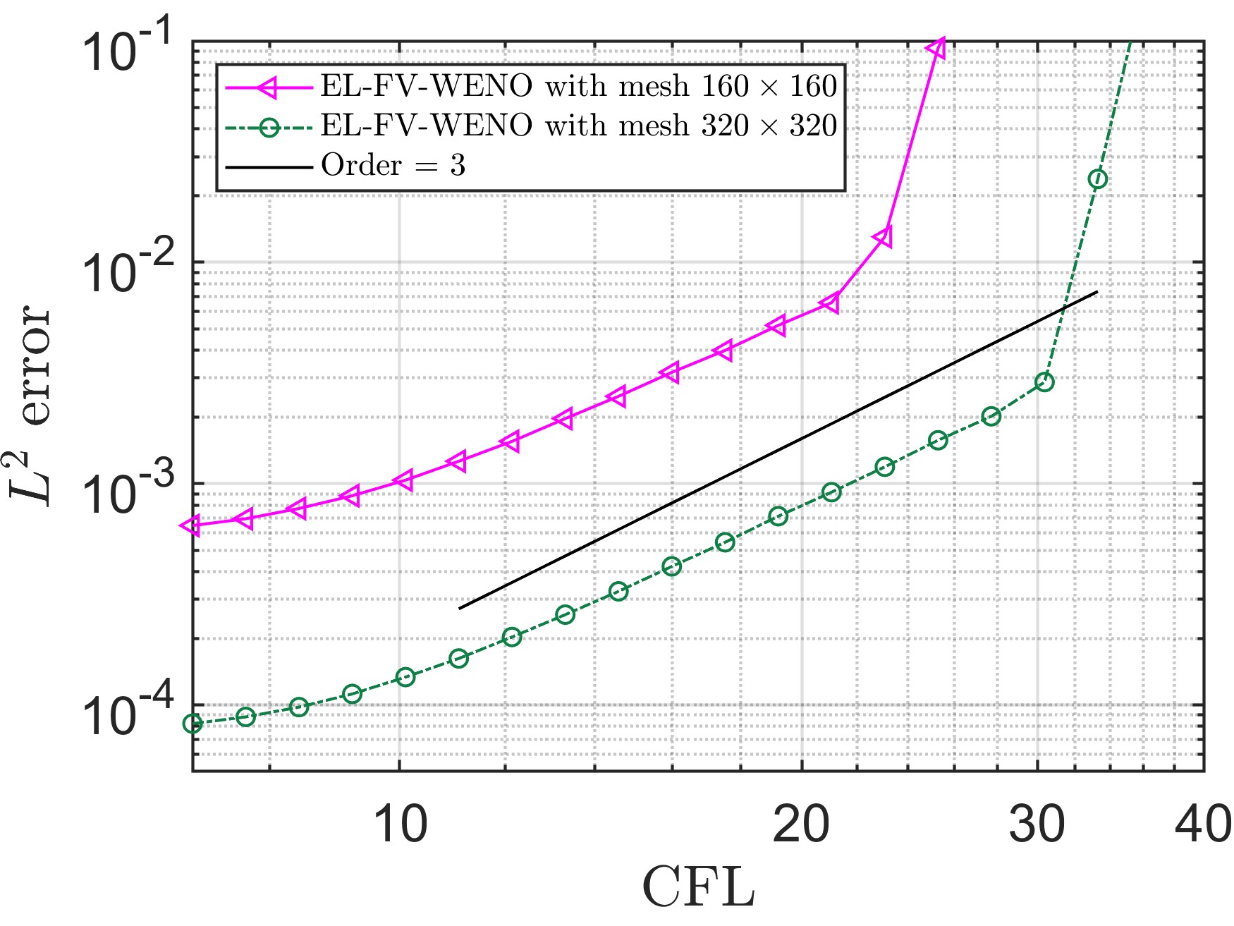
Figure 4: (Swirling deformation flow) Log-log plot of CFL numbers versus $L^{2}$ errors with fixed meshes $160\times 160$ and $320\times 320$ at $t=1.5$ of the EL-RK-FV-WENO scheme.

To validate the non-oscillatory nature of the proposed WENO reconstruction, we consider a discontinuous initial condition featuring a cylinder with a notch, a cone, and a smooth bell as shown in Figure 5. Figures 6 and 7 display the mesh plots and contour plots of the numerical solutions at $t=0.75$ and $t=1.5$. The swirling deformation flow significantly deforms the solution at half the period ($t=0.75$) and then reforms it back to its initial state at $t=1.5$. The WENO reconstruction method effectively controls numerical oscillations as demonstrated.

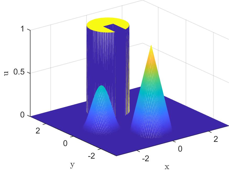
(a) Mesh plot

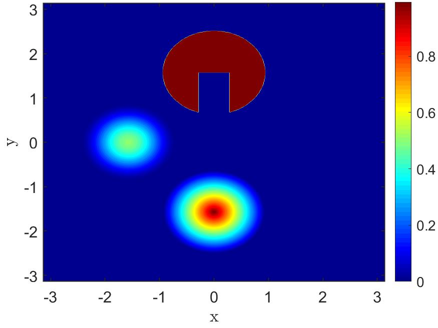
(b) Contour plot

Figure 5: (Swirling deformation flow) Mesh plot and contour plot of a discontinuous initial condition.

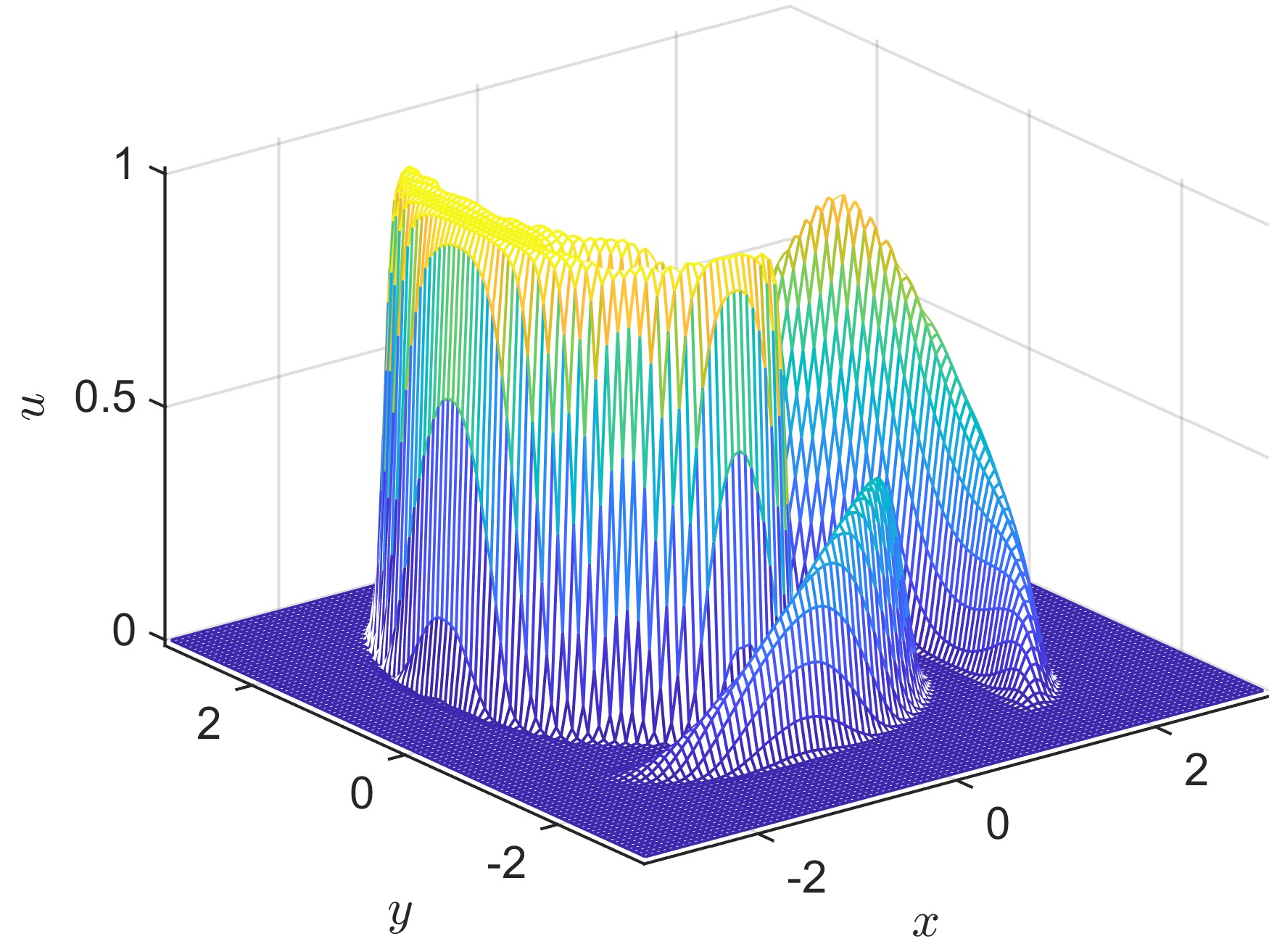
(a) Mesh plot

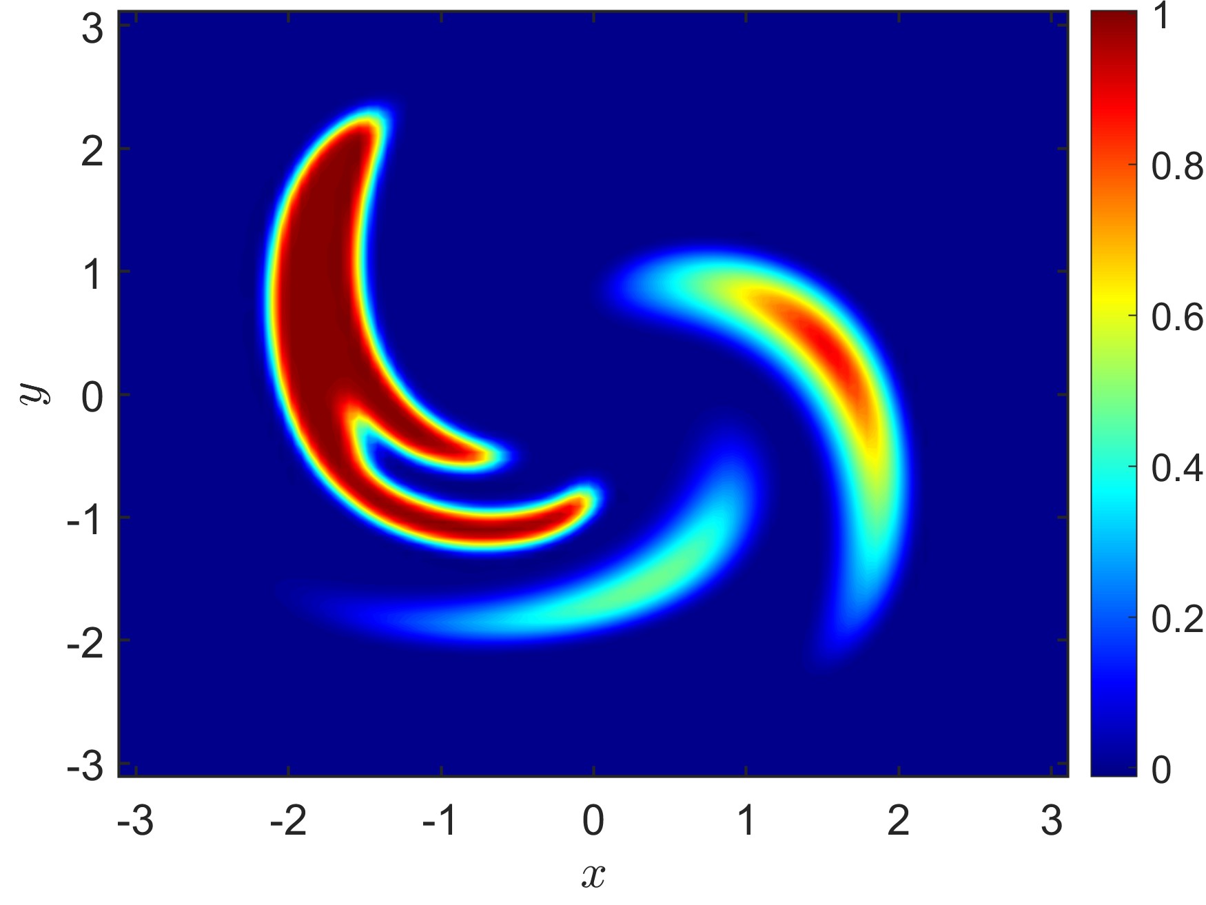
(b) Contour plot

Figure 6: (Swirling deformation flow) Mesh plot and contour plot of the numerical solution of the EL-RK-FV-WENO scheme with CFL = 10.2 and mesh size $100\times 100$ at $t=0.75$.

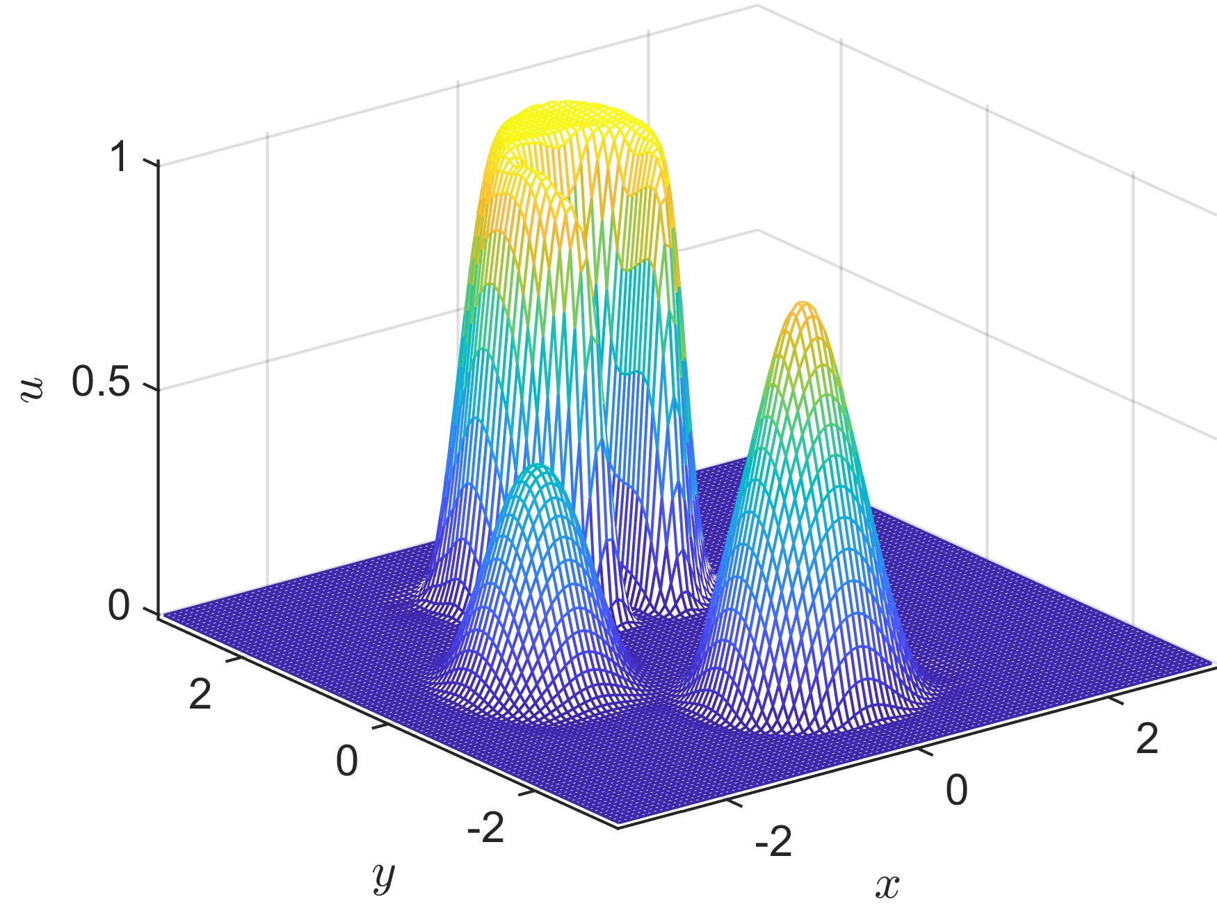
(a) Mesh plot

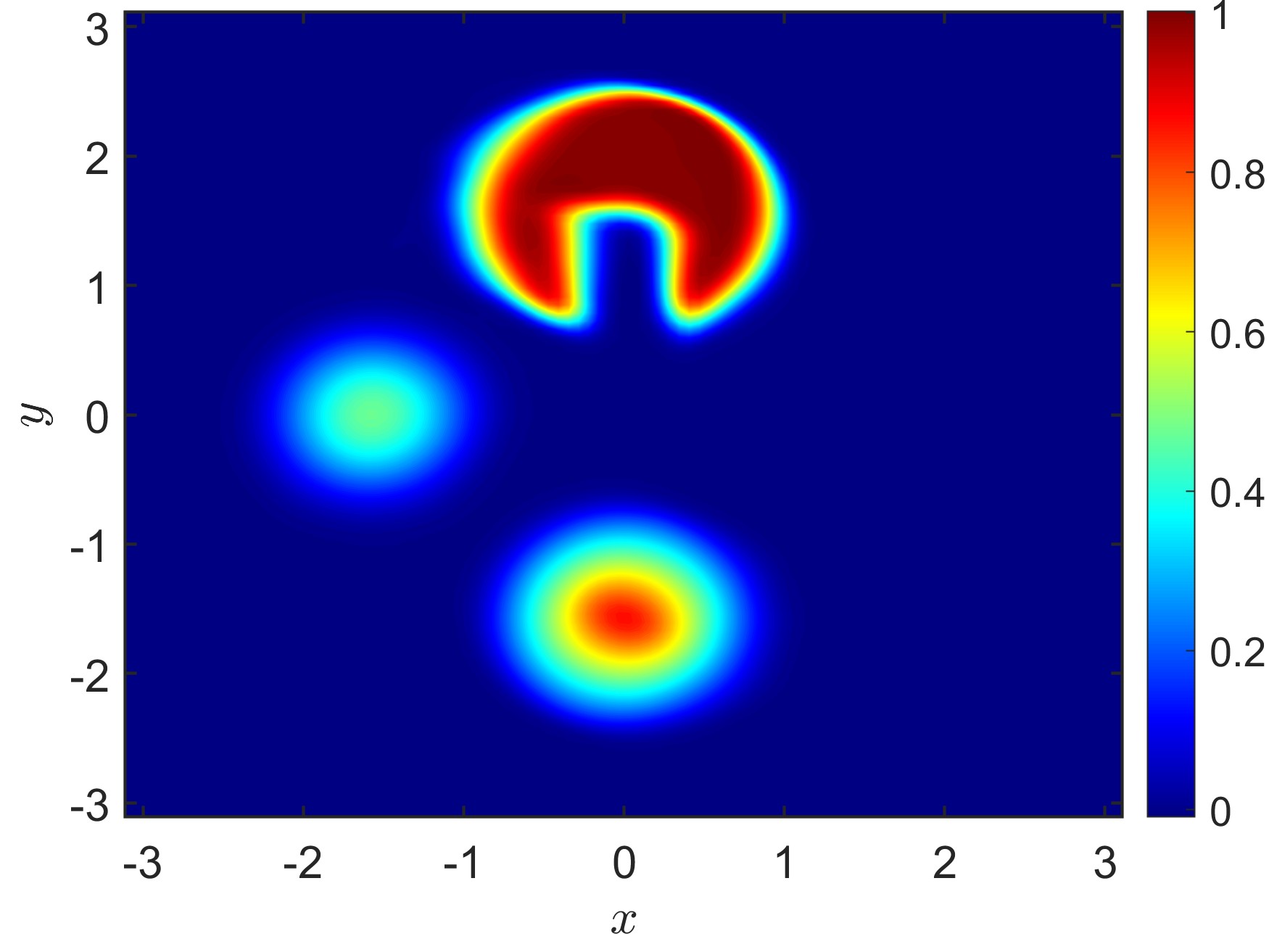
(b) Contour plot

Figure 7: (Swirling deformation flow) Mesh plot and contour plot of the numerical solution of the EL-RK-FV-WENO scheme with CFL = 10.2 and mesh size $100\times 100$ at $t=1.5$.

In summary, this example illustrates the effectiveness of the proposed EL-RK-FV evolving strategy for the convection terms. This strategy, which involves remapping from Eulerian to Lagrangian spatial approximations, not only achieves high-order spatial and temporal accuracy but also allows for large time-steps while maintaining a non-oscillatory property.

Example 3.2.

(The 0D2V Leonard-Bernstein linearized Fokker-Planck equation) Consider the following equation:

(46) $$f_{t}+\frac{1}{\epsilon}\left((v_{x}-\overline{v}_{x})f\right)_{v_{x}}-\frac{1}{\epsilon}\left((v_{y}-\overline{v}_{y})f\right)_{v_{y}}=\frac{1}{\epsilon}D\left(f_{v_{x}v_{x}}+f_{v_{y}v_{y}}\right),~{}~{}~{}~{}v_{x},v_{y}\in[-2\pi,2\pi]$$

with zero boundary conditions and an equilibrium solution by the given Maxwellian:

(47) $$f_{M}(v_{x},v_{y})=\frac{n}{2\pi RT}\exp\left(\frac{(v_{x}-\overline{v}_{x})^{2}+(v_{y}-\overline{v}_{y})^{2}}{2RT}\right),$$

where, $\epsilon=1$, gas constant $R=1/6$, temperature $T=3$, thermal velocity $v_{th}=\sqrt{2RT}=\sqrt{2D}=1$, number density $n=\pi$, and bulk velocities $\overline{v}_{x}=\overline{v}_{y}=1$. For spatial and temporal accuracy tests, we choose $f(v_{x},v_{y},0)=f_{M}(v_{x},v_{y})$. In Table 2, we present the $L^{1}$, $L^{2}$, and $L^{\infty}$ errors and the corresponding orders of accuracy for the proposed scheme. The results demonstrate a consistent 3rd-order spatial accuracy.

Table 2: (The 0D2V Leonard-Bernstein linearized Fokker-Planck equation) $L^{1}$, $L^{2}$, and $L^{\infty}$ errors and corresponding orders of accuracy of the EL-RK-FV-WENO scheme for (46) with initial condition (47) at $t=0.5$ with CFL = 1.

mesh	$L^{1}$ error	order	$L^{2}$ error	order	$L^{\infty}$ error	order
20$\times$ 20	2.18E-03	—	1.38E-02	—	2.95E-01	—
40$\times$ 40	3.01E-04	2.85	2.05E-03	2.75	9.50E-02	1.63
80$\times$ 80	3.33E-05	3.18	1.58E-04	3.70	6.40E-03	3.89
160$\times$ 160	4.10E-06	3.02	1.80E-05	3.13	2.88E-04	4.47
320$\times$ 320	4.77E-07	3.10	2.10E-06	3.11	3.20E-05	3.17

By fixing the spatial mesh and varying the CFL number, the temporal order of accuracy is investigated in Figure 8. The proposed scheme exhibits 3rd-order temporal accuracy and allows the use of large time-steps, as evidenced by the stability for high CFL numbers.

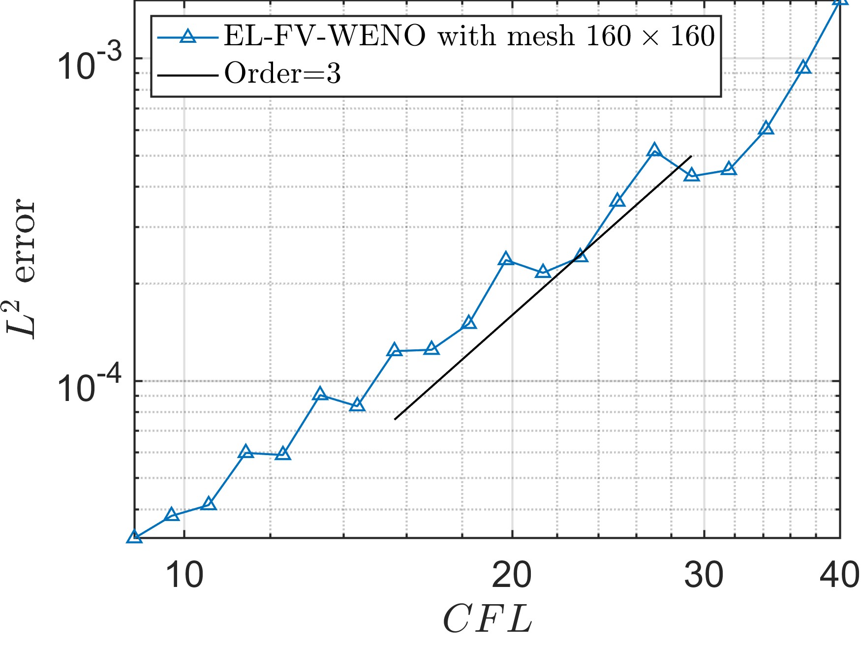
Figure 8: (The 0D2V Leonard-Bernstein linearized Fokker-Planck equation) Log-log plot of CFL numbers versus $L^{2}$ errors with fixed mesh $160\times 160$ at $t=0.5$ for the EL-RK-FV-WENO scheme.

To test the relaxation of the system, we choose the initial condition $f(v_{x},v_{y},t=0)=f_{M1}(v_{x},v_{y})+f_{M2}(v_{x},v_{y})$, where the parameters of each Maxwellian, $f_{M1}$ and $f_{M2}$, are detailed in Table 3. The two Maxwellians are shifted along the $v_{x}$ direction with $\overline{v}_{y}=0$. The evolution of the numerical results, illustrated in Figure 9, shows that after $t\geq 3$, there is no discernible difference between the numerical solution and the solution at $t=3$, validating the efficacy of the proposed scheme.

	$f_{M1}$	$f_{M2}$
$n$	1.990964530353041	1.150628123236752
$\bar{v}_{x}$	0.4979792385268875	-0.8616676237412346
$\bar{v}_{y}$	0	0
$T$	2.46518981703837	0.4107062104302872

Table 3: (The 0D2V Leonard-Bernstein linearized Fokker-Planck equation) Settings of the Maxwellians $f_{M1}$ and $f_{M2}$.

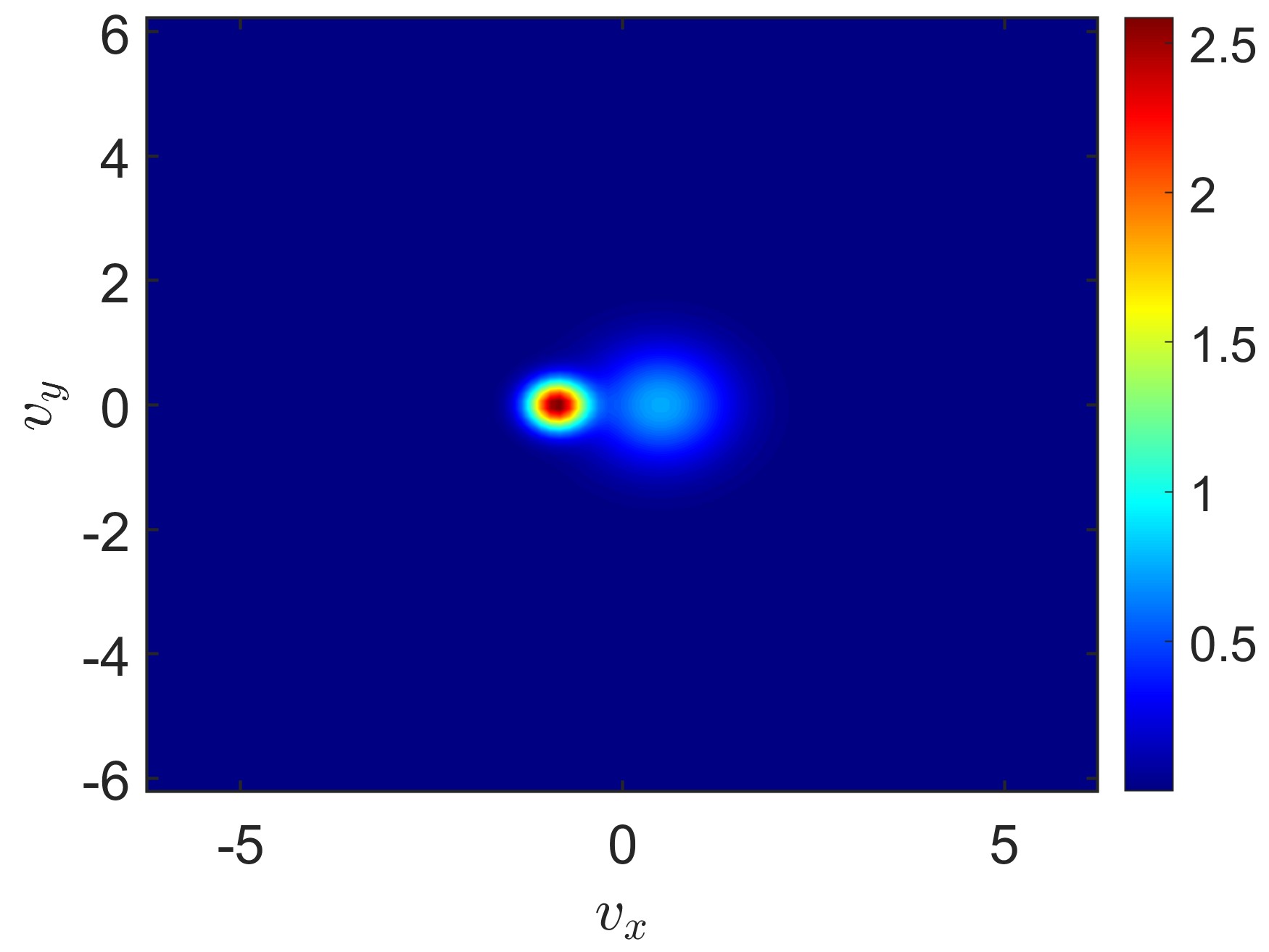
(a) $t=0$

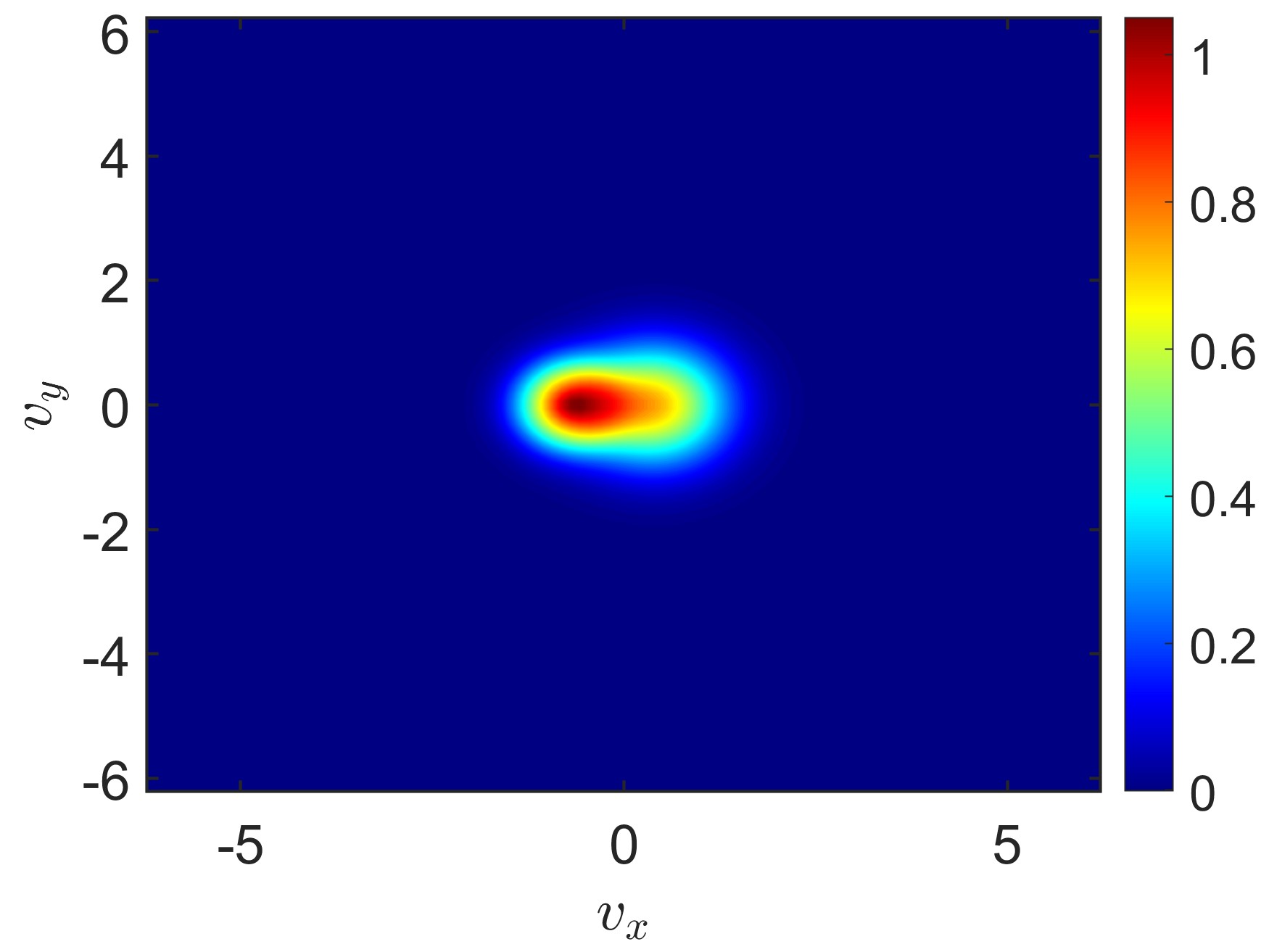
(b) $t=0.2$

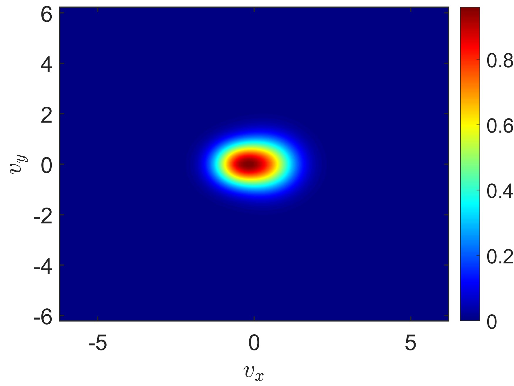
(c) $t=0.4$

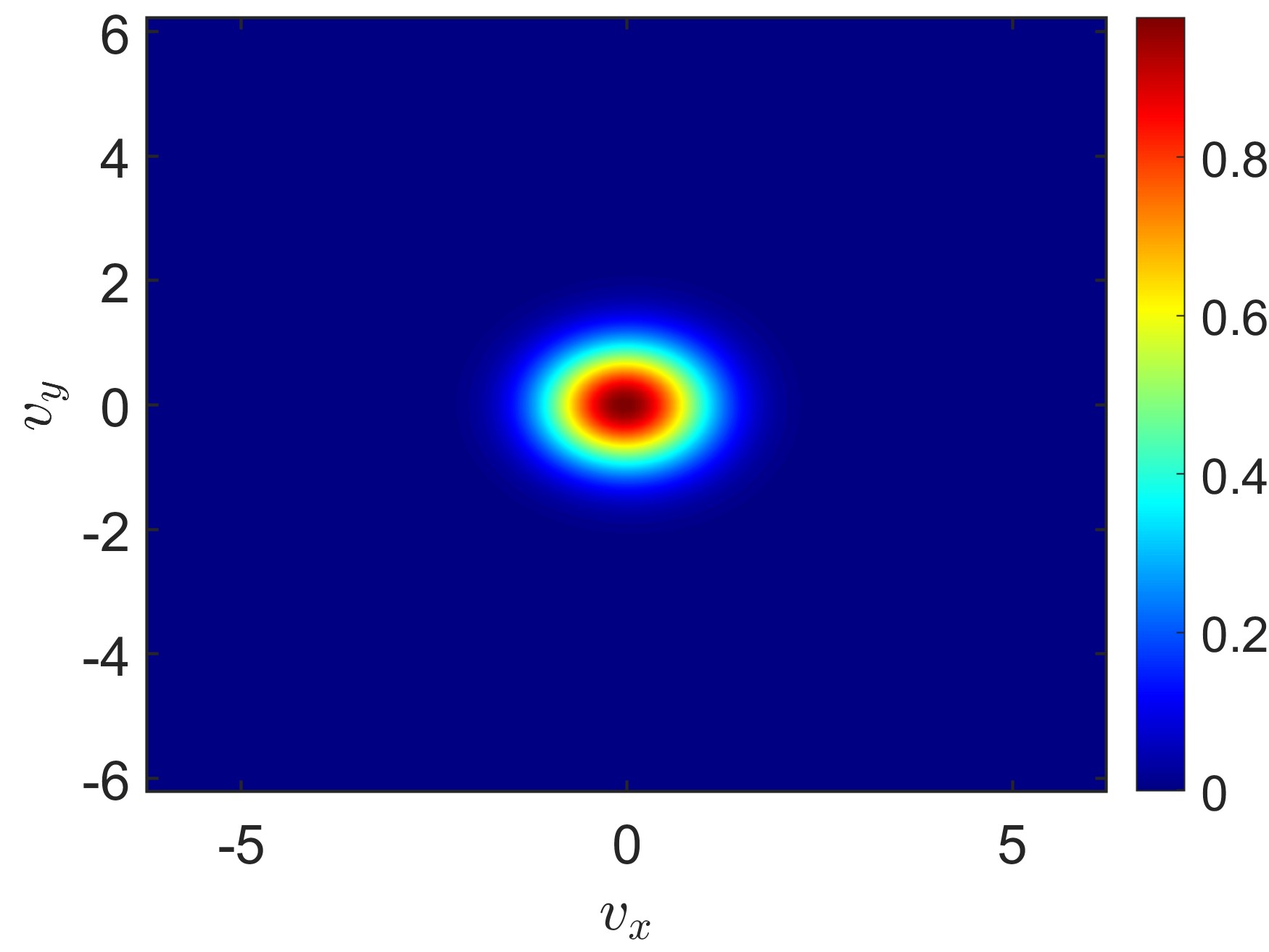
(d) $t=0.8$

(e) $t=3$

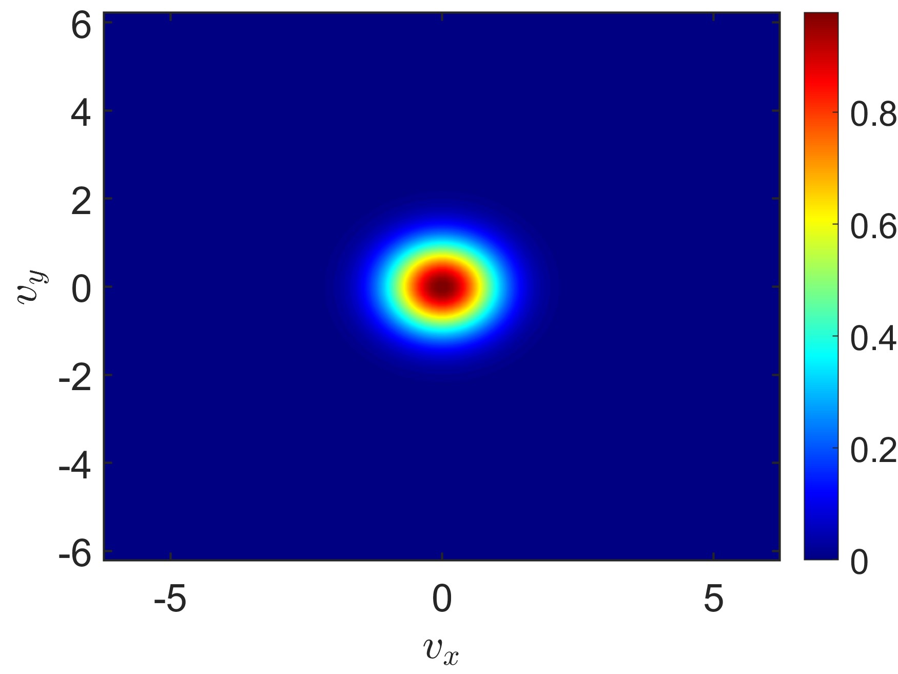
(f) $t=20$

Figure 9: (The 0D2V Leonard-Bernstein linearized Fokker-Planck equation) Contour plots of the numerical results of the EL-RK-FV-WENO scheme with CFL = 3 and mesh size $100\times 100$ at $t=0$ (initial condition), $t=0.2$, $t=0.4$, $t=0.6$, $t=3$, and $t=20$.

In Figure 10, we present the capability of the proposed scheme in preserving various physical conservative quantities. The results indicate that while the scheme is effective in conserving mass, it does not maintain the other quantities to the machine precision.

(a)

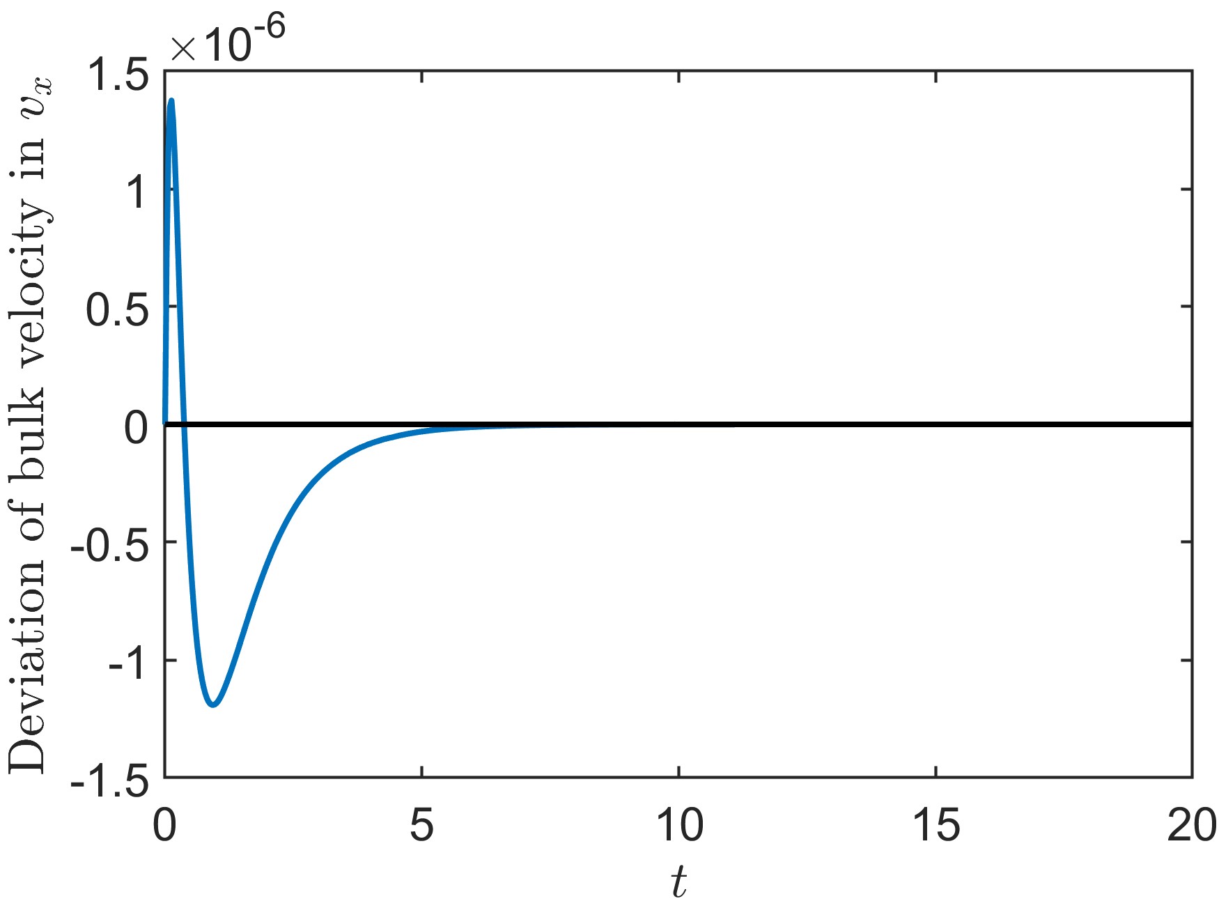
(b)

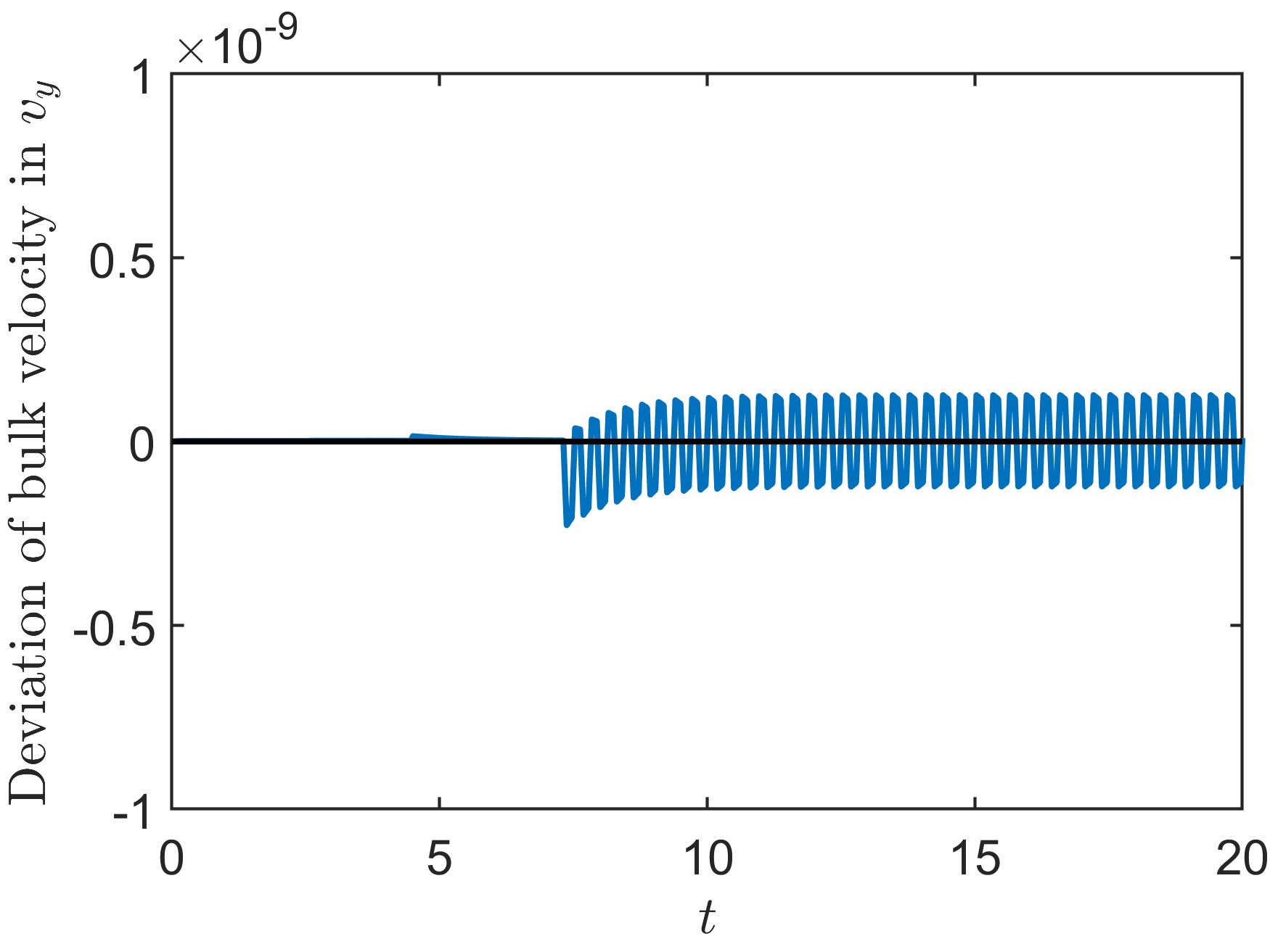
(c)

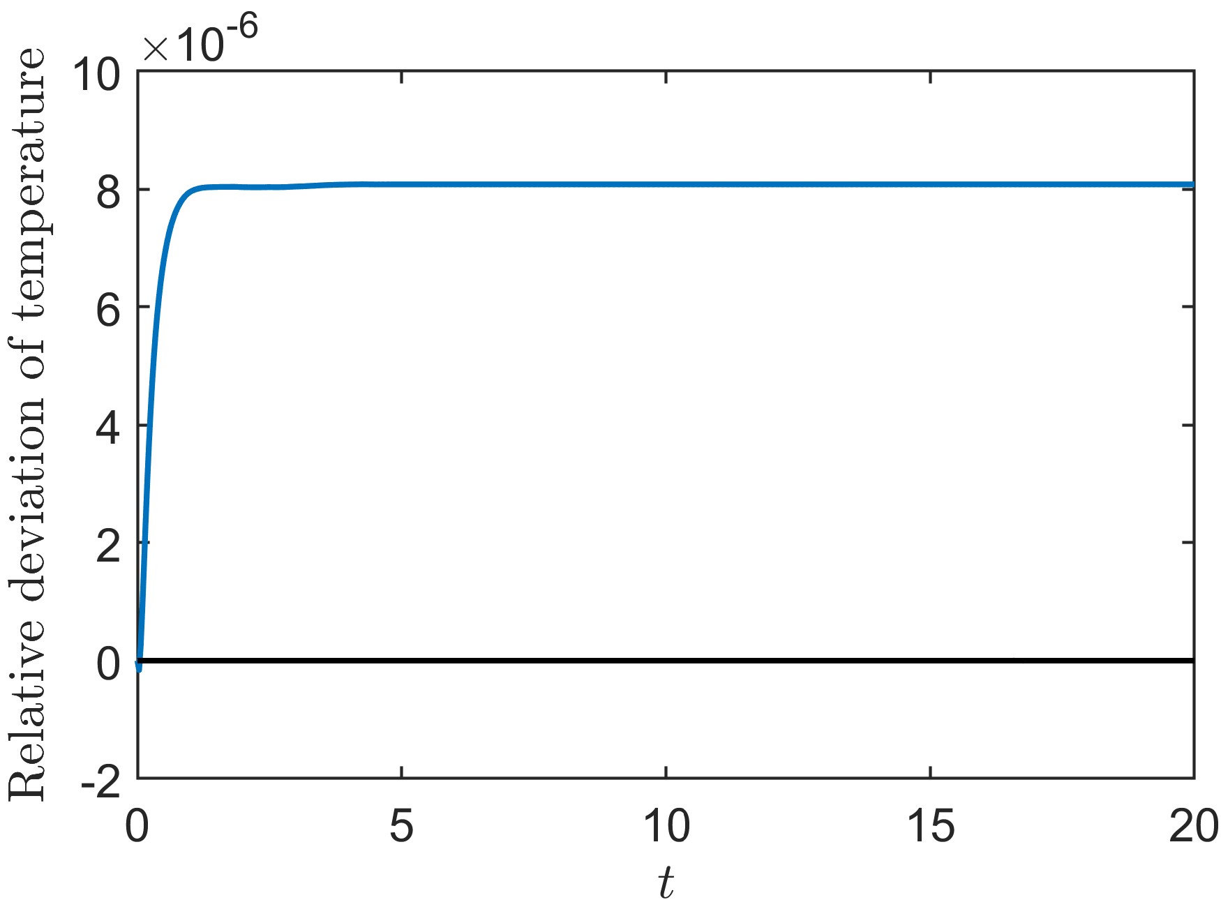
(d)

Figure 10: (The 0D2V Leonard-Bernstein linearized Fokker-Planck equation) Relative deviation (or deviation) of number density, bulk velocity in $v_{x}$, bulk velocity in $v_{y}$, and temperature for the EL-RK-FV-WENO scheme with CFL = 10.2 and with mesh $160\times 160$ from $t=0$ to $t=20$ .

To encapsulate, this example primarily demonstrates the effectiveness of the IMEX temporal discretization, which combines the implicit solver for the diffussion term and the EL evolving strategy for the convection terms, enabling the use of large time-steps.

3.2 Nonlinear models

Example 3.3.

(Kelvin-Helmholtz instability problem) Consider the guiding center Vlasov model [26, 15]:

(48) $$\begin{split}\rho_{t}+\nabla\cdot(\mathbf{E}^{\perp}\rho)=0,\\ -\Delta\Phi=\rho,~{}~{}\mathbf{E}^{\perp}=\left(-\Phi_{y},\Phi_{x}\right),\end{split}$$

with the periodic boundary condition and the following initial condition:

(49) $$\begin{split}\rho(x,y,0)=\text{sin}(y)+0.015\text{cos}(0.5x),~{}~{}x\in[0,4\pi],~{}~{}y\in[0,2\pi],\end{split}$$

where $\rho$ is the charge density and $\mathbf{E}$ is the electric field. We validate the 3rd-order spatial and temporal accuracy of the proposed scheme in Table 4 and Figure 11. Additionally, the stability of the scheme with large time-steps up to CFL = 50 is verified.

Table 4: (Kelvin-Helmholtz instability problem) $L^{1}$, $L^{2}$, and $L^{\infty}$ errors and corresponding orders of accuracy of the EL-RK-FV-WENO scheme for (48) with initial condition (49) at $t=5$ with CFL = 1.

mesh	$L^{1}$ error	order	$L^{2}$ error	order	$L^{\infty}$ error	order
16$\times$ 16	6.79E-03	—	1.11E-02	—	6.68E-02	—
32$\times$ 32	5.48E-04	3.63	9.46E-04	3.55	1.18E-02	2.50
64$\times$ 64	4.35E-05	3.66	7.15E-05	3.73	1.43E-03	3.05
128$\times$ 128	4.37E-06	3.31	6.45E-06	3.47	1.98E-04	2.85
256$\times$ 256	5.23E-07	3.06	6.72E-07	3.26	1.73E-05	3.51

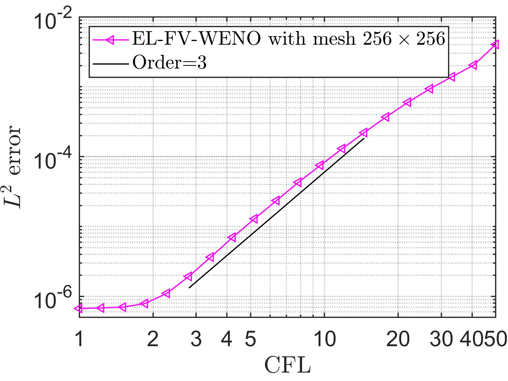
Figure 11: (Kelvin-Helmholtz instability problem) Log-log plot of CFL numbers versus $L^{2}$ errors with fixed mesh $256\times 256$ at $t=5$ of the EL-RK-FV-WENO scheme.

In Figure 12, we display the mesh plot and contour plot of the numerical solution of the EL-RK-FV-WENO scheme at $t=40$. The result is comparable with the one of our fourth-order SL-FV-WENO scheme in [37].

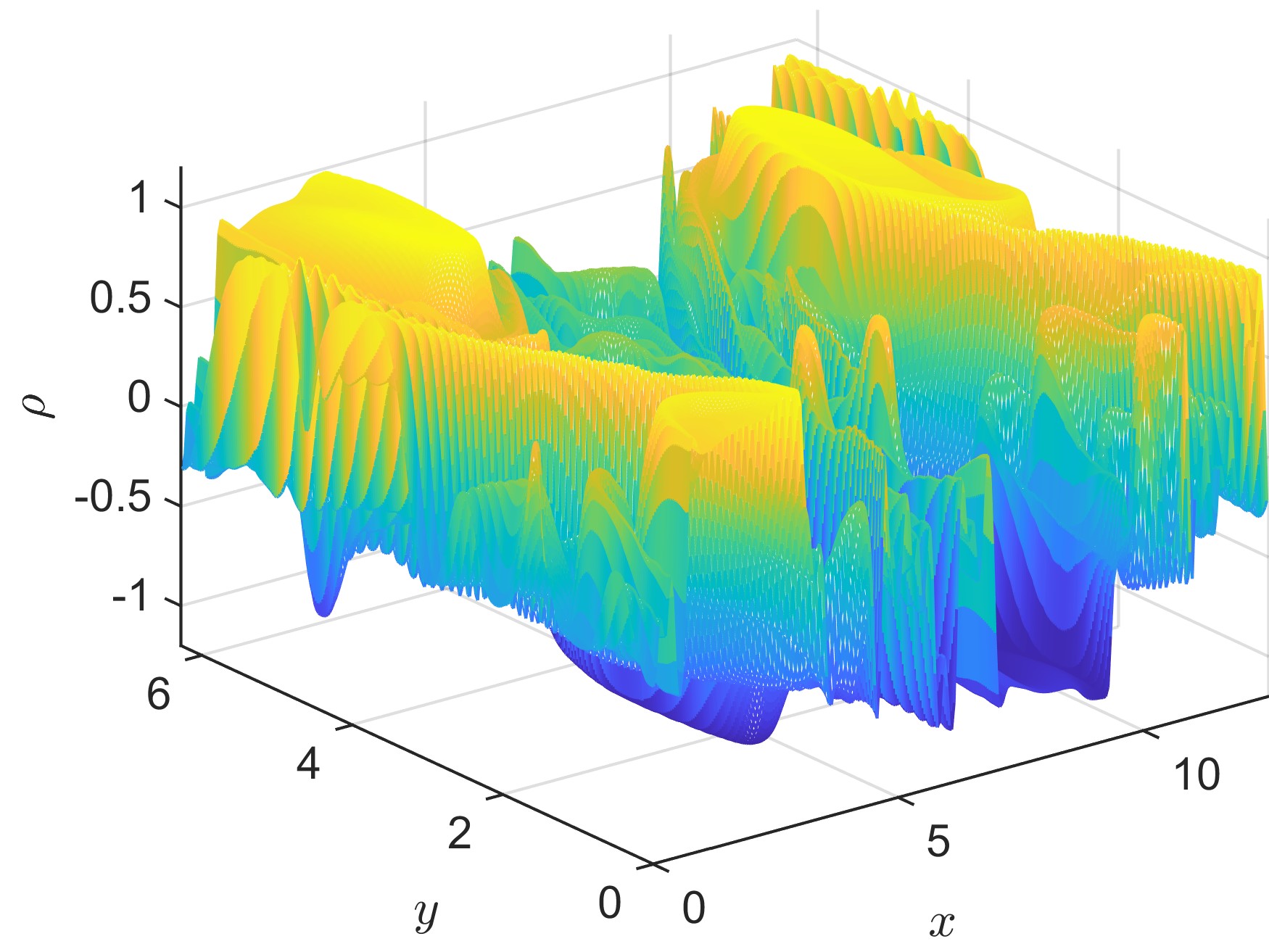
(a) Mesh plot

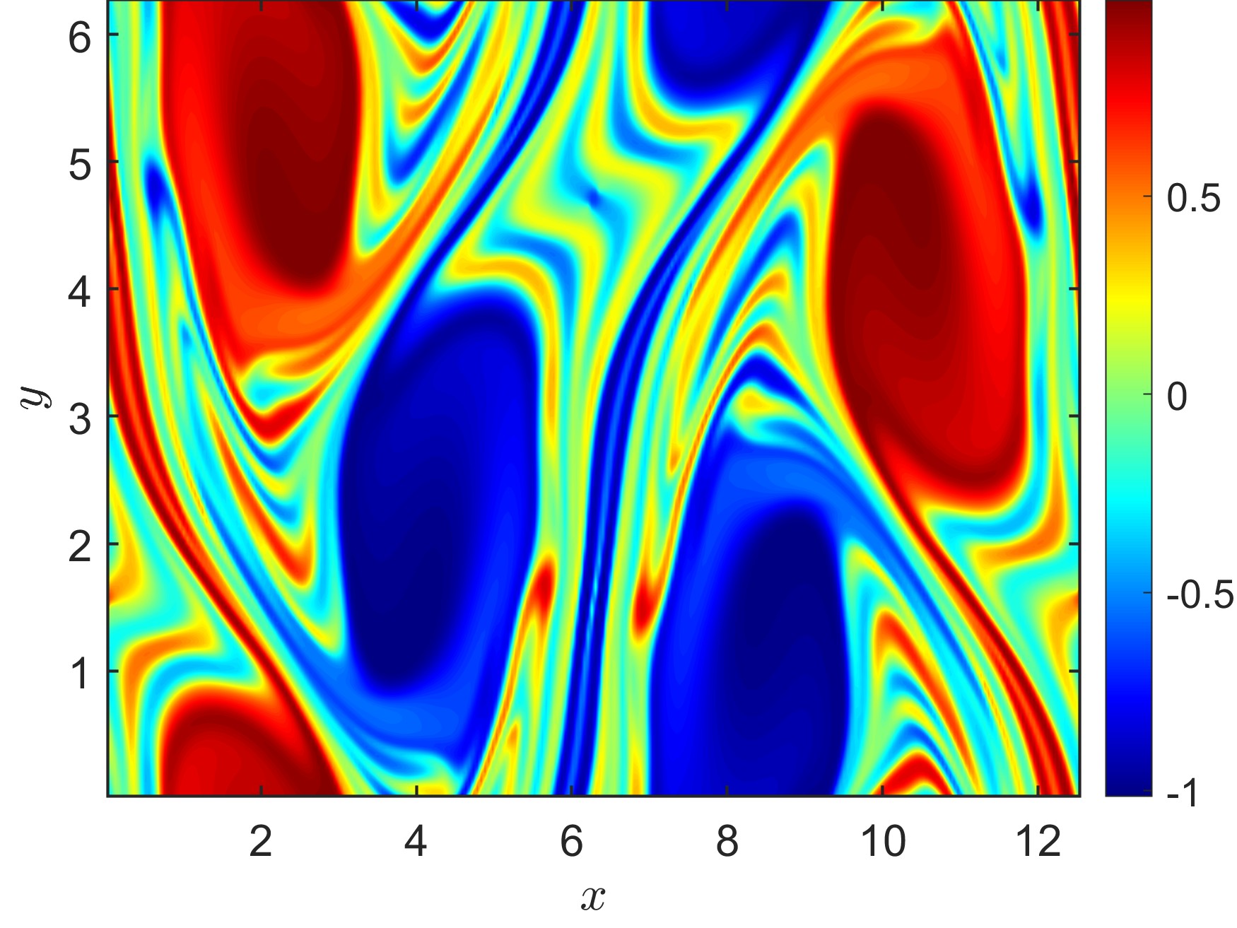
(b) Contour plot

Figure 12: (Kelvin-Helmholtz instability problem) Mesh plot and contour plot of the numerical solution of the EL-RK-FV-WENO scheme with CFL = 10.2 and with mesh $256\times 256$ at $t=40$.

In Figure 13, we show the deviation of mass, relative deviation of energy and entropy of the proposed scheme from $t=0$ to $t=50$. As shown, the proposed scheme is mass conservative. The magnitudes of relative deviation of energy and entropy results are comparable with the ones in [37].

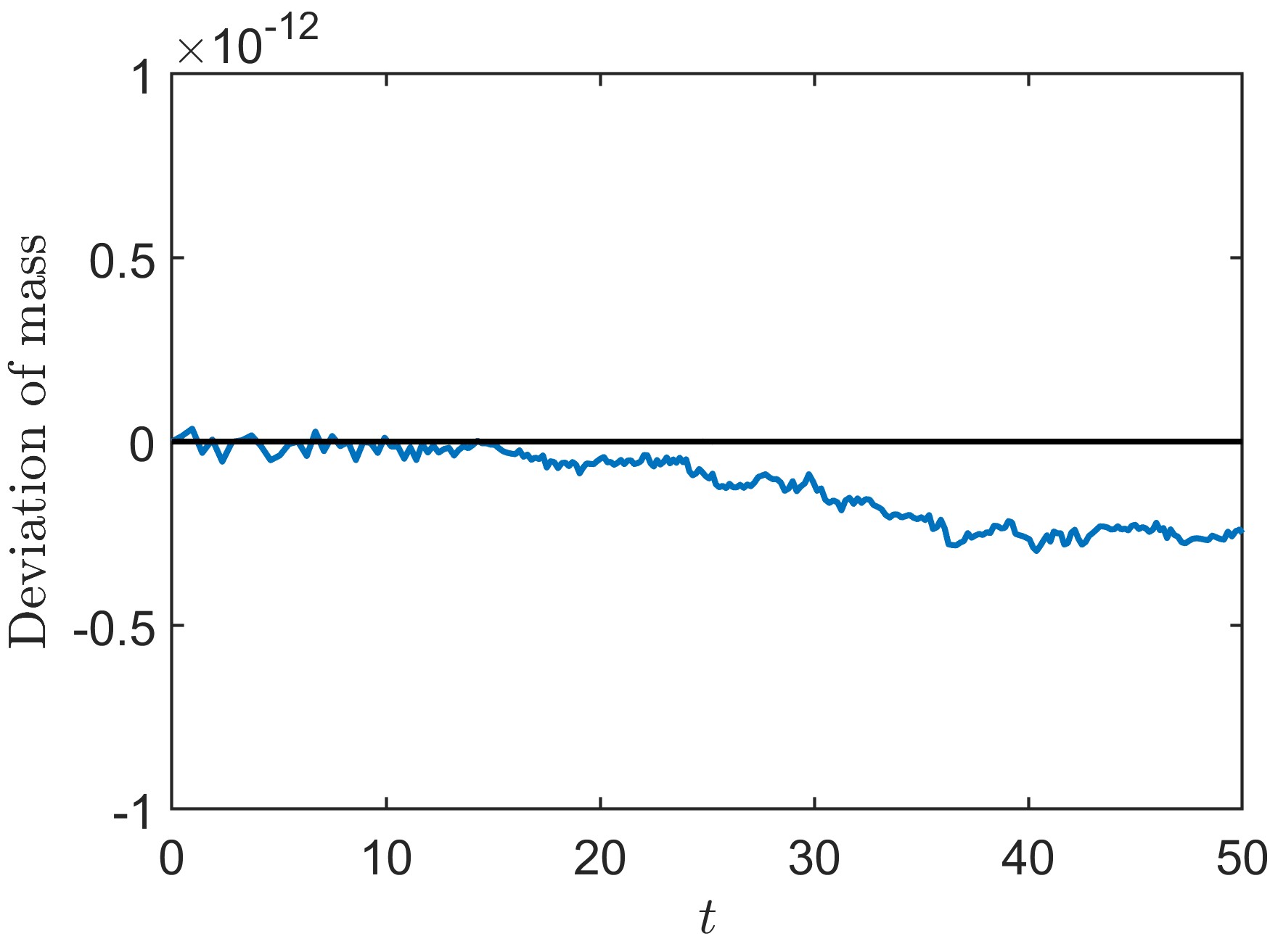
(a) Deviation of mass

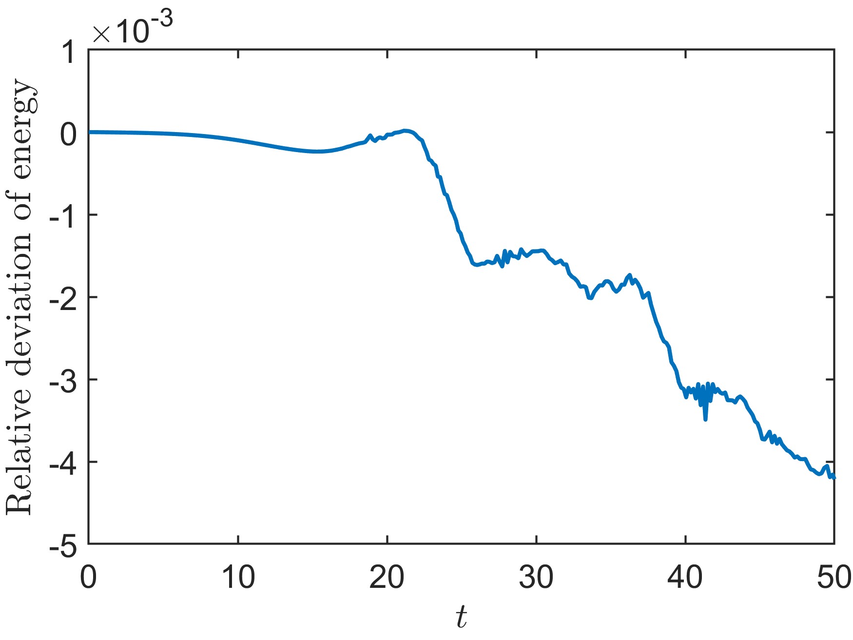
(b) Relative deviation of energy

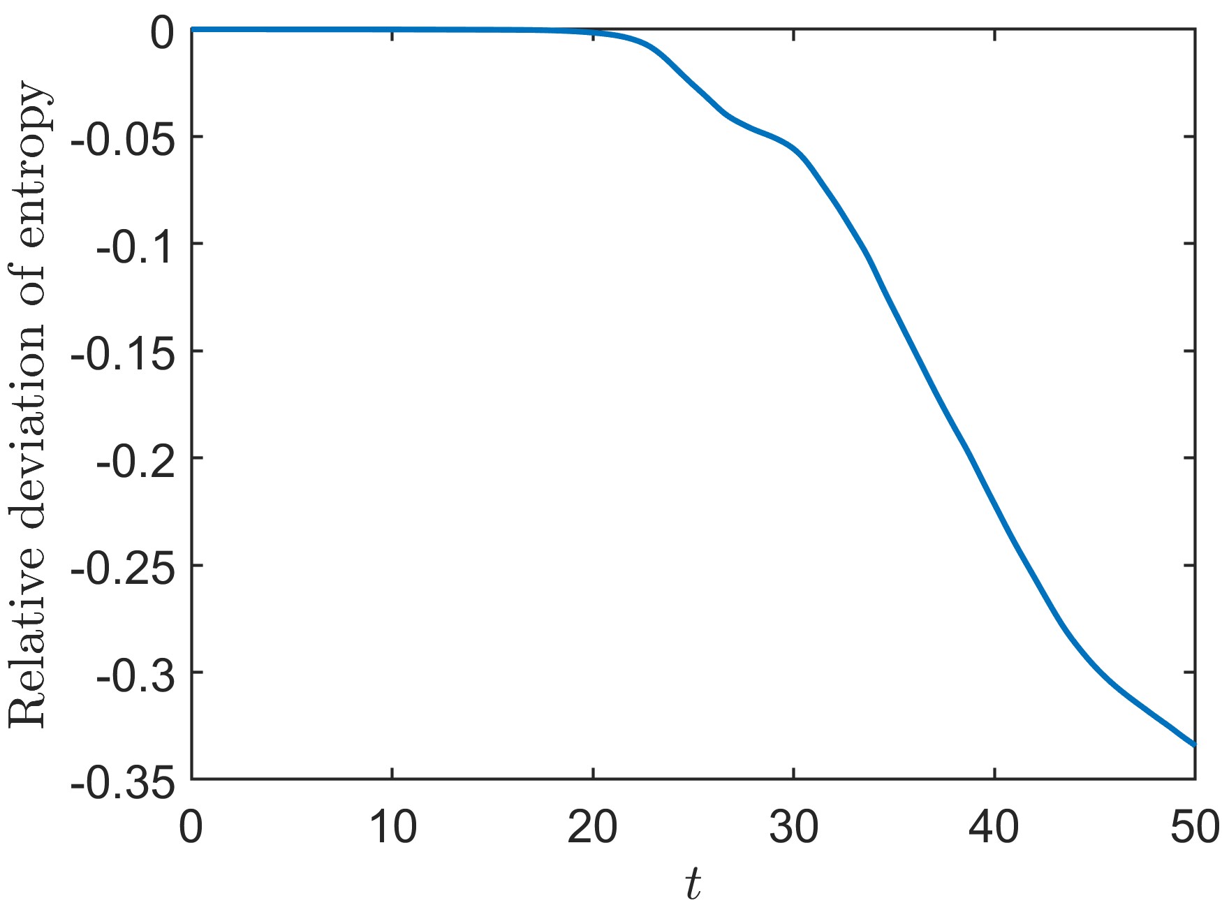
(c) Relative deviation of entropy

Figure 13: (Kelvin-Helmholtz instability problem) Deviation of mass, relative deviation of energy and entropy for the EL-RK-FV-WENO scheme with CFL = 10.2 and with mesh $256\times 256$ from $t=0$ to $t=50$ .

This nonlinear example effectively showcases the success of the generalization strategy for nonlinear model outlined in Section 2.3, which is achieved with minimal additional cost.

Example 3.4.

(Incompressible Navier-Stokes equations) The governing equations are as follows:

(50) $$\begin{split}\omega_{t}+(u\omega)_{x}+(v\omega)_{y}=\nu(\omega_{xx}+\omega_{yy}),\\ \Delta\psi=\omega,~{}~{}\left(u,v\right)=\left(\psi_{y},\psi_{x}\right),\end{split}$$

where $\omega$ is the vorticity of the flow, $\left(u,v\right)$ is the velocity field, and $\nu$ is the kinematic viscosity, which is set to be $\frac{1}{100}$. We first consider an initial condition given by:

(51) $$\omega(x,y,0)=-2\sin(x)\sin(y),\quad x\in[0,2\pi],~{}~{}y\in[0,2\pi]$$

with the exact solution $\omega(x,y,t)=-2\sin(x)\sin(y)\exp(-2t\nu)$. Similarly, 3rd-order spatial and temporal order of accuracy of validated in Table 5 and Figure 14 respectively. For this problem, we observe that large time-steps are allowed for the proposed scheme up to CFL = 40.

Table 5: (Incompressible Navier-Stokes equations) $L^{1}$, $L^{2}$, and $L^{\infty}$ errors and corresponding orders of accuracy of the EL-RK-FV-WENO scheme for (50) with initial condition (51) at $t=0.5$ with CFL = 1.

mesh	$L^{1}$ error	order	$L^{2}$ error	order	$L^{\infty}$ error	order
16$\times$ 16	3.90E-03	—	4.65E-03	—	1.14E-02	—
32$\times$ 32	4.88E-04	3.00	5.82E-04	3.00	1.45E-03	2.98
64$\times$ 64	6.09E-05	3.00	7.27E-05	3.00	1.82E-04	2.99
128$\times$ 128	7.61E-06	3.00	9.08E-06	3.00	2.29E-05	2.99
256$\times$ 256	9.51E-07	3.00	1.13E-06	3.00	2.86E-06	3.00

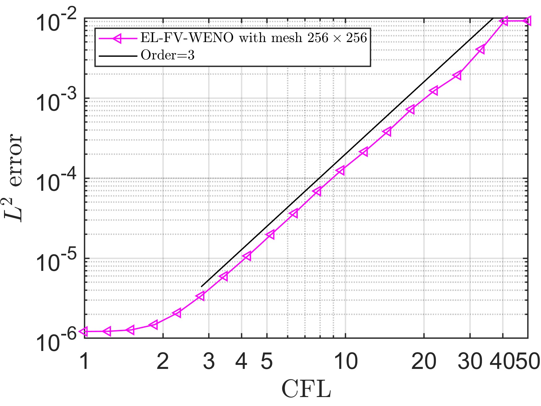
Figure 14: (Incompressible Navier-Stokes equations) Log-log plot of CFL numbers versus $L^{2}$ errors with fixed mesh $256\times 256$ at $t=0.5$ of the EL-RK-FV-WENO scheme.

For a more complex scenario, we consider the incompressible Navier-Stokes equation (50) on $[0,2\pi]^{2}$ with the following initial condition (the vortex patch problem)

(52) $$\omega(x,y,0)=\begin{cases}-1,\quad\frac{\pi}{2}\leq x\leq\frac{3\pi}{2},~{}~{}\frac{\pi}{4}\leq y\leq\frac{3\pi}{4};\\ 1,\quad~{}~{}\frac{\pi}{2}\leq x\leq\frac{3\pi}{2},~{}~{}\frac{5\pi}{4}\leq y\leq\frac{7\pi}{4};\\ 0\quad~{}~{}~{}~{}\text{otherwise}\end{cases}$$

with zero boundary condition. We provide the mesh plot and contour plot of the numerical solution of the proposed scheme at $t=5$ in Figure 15. The numerical result in Figure 15 is comparable with the one in [34].

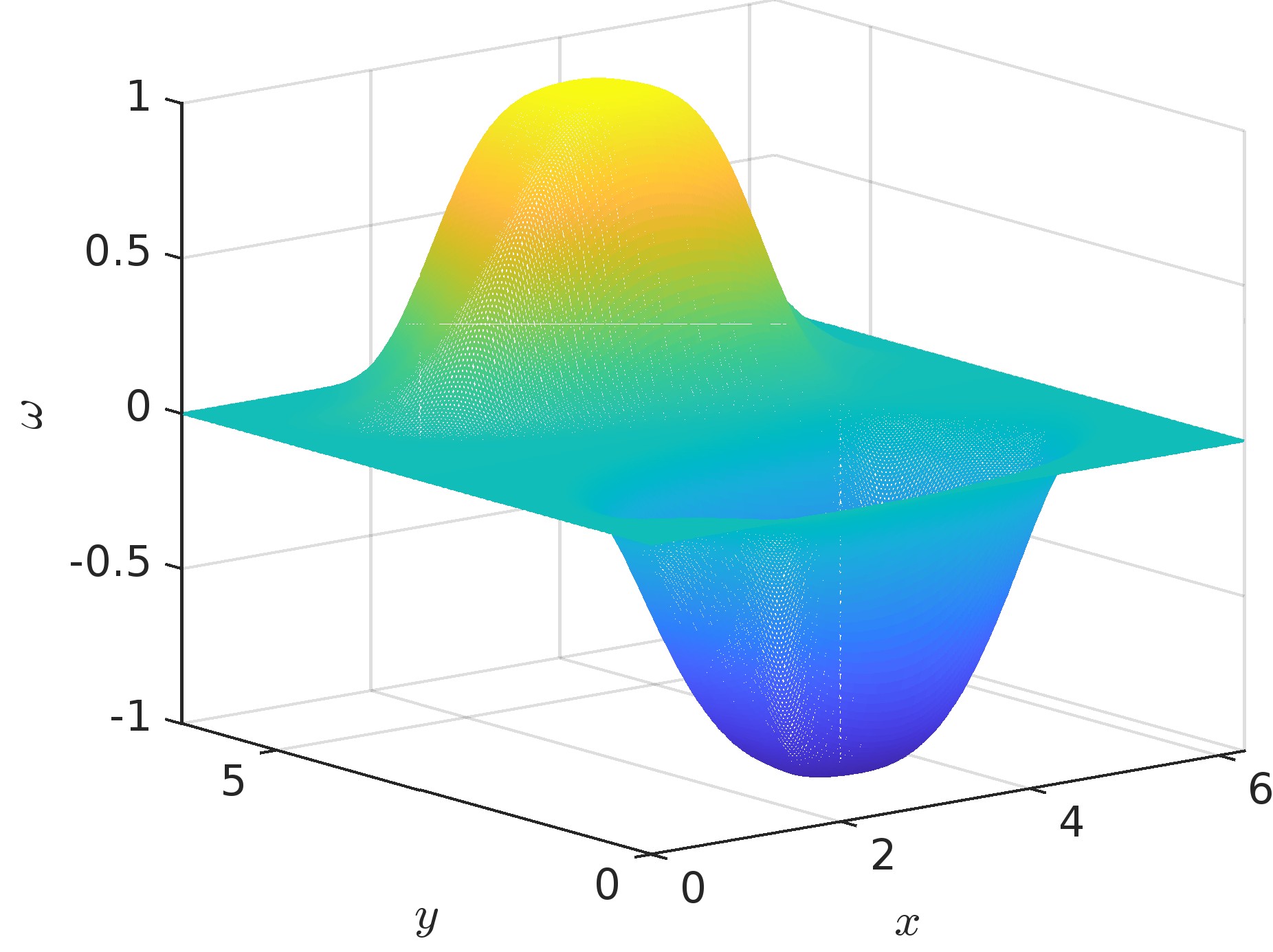
(a) Mesh plot

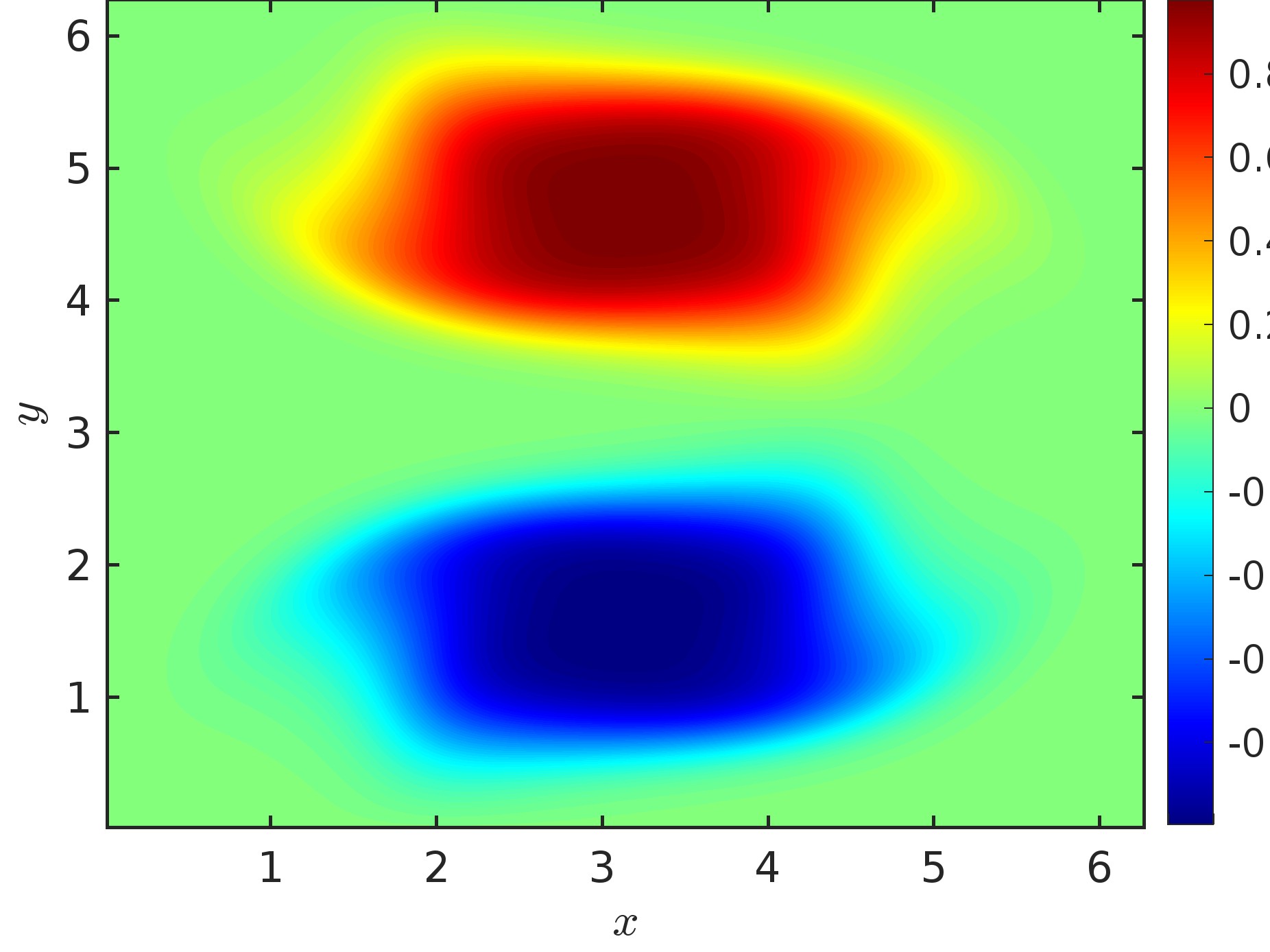
(b) Contour plot

Figure 15: (Vortex patch problem) Mesh plot and contour plot of the numerical solution of the EL-RK-FV-WENO scheme with CFL = 10.2 and with mesh $256\times 256$ at $t=5$.

Reflecting on this example, we note that the proposed EL-RK-FV-WENO scheme is able to simulate a nonlinear convection-diffusion equation with all the designed good properties. This is one of the major reasons why this EL-RK-FV-WENO scheme is attractive compared with our previous SL-FV-WENO scheme [37].

4 Conclusion

In this paper, we introduce a third-order EL-RK-FV-WENO scheme for convection-diffusion equations. By defining a modified velocity field and corresponding flux-form semi-discretization, we relax the time-step constraint. Spatial discretization is carefully designed to fit the EL formulation and overcome the challenges brought by the modified velocity field. Compared with the SL-FV scheme in [37], the proposed EL-RK-FV-WENO scheme is capable of simulating nonlinear convection-diffusion equations while inheriting the ability to apply large time-steps. Extensive numerical tests are conducted, verifying the effectiveness of the proposed scheme.

Appendix A Third-order WENO-ZQ reconstruction method for Eulerian mesh

In this appendix, we introduce the 3rd-order WENO-ZQ reconstruction for the Eulerian mesh. For convenience, we assume $\Delta x_{i}\equiv\Delta x$ and $\Delta y_{j}\equiv\Delta y$ for all $i,~{}j$. We define $\mu_{i}(x):=\frac{x-x_{i}}{\Delta x}$, $\nu_{j}(y):=\frac{y-y_{j}}{\Delta y}$ and introduce a set of local orthogonal polynomials as $\{P^{(i,j)}_{l}(x,y)\}$ for a given cell $I_{i,j}$:

(53) $$P^{(i,j)}_{1}:=1,\quad P^{(i,j)}_{2}:=\mu_{i}(x),\quad P^{(i,j)}_{3}:=\nu_{j}(y),$$

$$P^{(i,j)}_{4}:=\mu_{i}^{2}(x)-\frac{1}{12},\quad P^{(i,j)}_{5}:=\mu_{i}(x)\nu_{j}(y),\quad P^{(i,j)}_{6}:=\nu_{j}^{2}(y)-\frac{1}{12}.$$

We assume that $\overline{u}_{5}:=\overline{u}_{i,j}$ and $I_{5}:=I_{i,j}$, while $\{u_{s}\}$ and $\{I_{s}\}$ represent corresponding cell averages and Eulerian cells based on the serial number in Figure 16. The reconstruction procedure is performed as follows:

Figure 16: Stencil for the 3rd-order WENO-ZQ reconstruction.

1. Construct a quadratic polynomial $q_{0}(x,y)=\sum\limits_{l=1}^{6}a_{l}^{q_{0}}P_{l}^{(i,j)}(x,y)$ using a special least-squares procedure. We define

   $$V:=\{p(x,y)\in P^{2}(I_{i,j})|\frac{1}{\Delta x\Delta y}\int_{I_{s}}p(x,y)dxdy=\overline{u}_{s},~{}s=2,4,5,6,8\},$$

   $$E(p(x,y)):=\left[\sum\limits_{s=1,3,7,9}\left(\frac{1}{\Delta x\Delta y}\int_{I_{s}}p(x,y)dxdy-\overline{u}_{s}\right)^{2}\right]^{\frac{1}{2}}.$$

   Then, we determine that $q_{0}(x,y)$ is the unique polynomial satisfying:

   (54) $$E(q_{0}(x,y))=\min\limits_{p\in V}{E(p(x,y))}.$$

2. Construct eight linear polynomials $\{q_{k}(x,y)\}_{k=1}^{8}=\{\sum\limits_{l=1}^{3}a_{l}^{q_{k}}P^{(i,j)}_{l}(x,y)\}$ satisfying:

   (55) $$\frac{1}{\Delta x\Delta y}\iint_{I_{5}}q_{k}(x,y)dxdy=\overline{u}_{5}\quad\text{for}~{}~{}k=1,2,\ldots,8,$$

   and

   (56) $$\frac{1}{\Delta x\Delta y}\iint_{I_{s}}q_{k}(x,y)dxdy=\overline{u}_{s},$$

   where

   $$\begin{split}&s=1,2\quad\text{for}~{}~{}k=1;~{}s=2,3\quad\text{for}~{}~{}k=2;\\ &s=3,6\quad\text{for}~{}~{}k=3;~{}s=6,9\quad\text{for}~{}~{}k=4;\\ &s=8,9\quad\text{for}~{}~{}k=5;~{}s=7,8\quad\text{for}~{}~{}k=6;\\ &s=4,7\quad\text{for}~{}~{}k=7;~{}s=1,4\quad\text{for}~{}~{}k=8.\\ \end{split}$$

3. Rewrite $q_{0}(x,y)$ as in [22, 23, 39]:

   (57) $$q_{0}(x,y)=\gamma_{0}\left(\frac{1}{\gamma_{0}}q_{0}(x,y)-\sum\limits_{k=1}^{8}\frac{\gamma_{k}{\gamma_{0}}}{q}_{k}(x,y)\right)+\sum\limits_{k=1}^{8}\gamma_{k}q_{k}(x,y),$$

   where $\{\gamma_{k}\}_{k=0}^{8}$ is a set of positive linear weights with their sum being $1$. The linear weights control the balance between optimal reconstruction accuracy and avoiding numerical oscillation. In our numerical tests, we set $\gamma_{0}=0.6$ and $\gamma_{1}=\ldots=\gamma_{8}=0.05$ for such balance.

4. Compute the smoothness indicators of $\{q_{k}(x,y)\}_{k=0}^{8}$ [19]:

   $$\begin{split}&\beta_{0}=\frac{1}{\Delta x\Delta y}\sum\limits_{l_{1}+l_{2}\leq 2}\iint_{I_{5}}\left(\Delta x^{l_{1}}\Delta y^{l_{2}}\frac{\partial^{|l_{1}+l_{2}|}}{\partial_{l_{1}}\partial_{l_{2}}}q_{0}(x,y)\right)^{2}dxdy,\\ &\beta_{k}=\frac{1}{\Delta x\Delta y}\sum\limits_{l_{1}+l_{2}\leq 1}\iint_{I_{5}}\left(\Delta x^{l_{1}}\Delta y^{l_{2}}\frac{\partial^{|l_{1}+l_{2}|}}{\partial_{l_{1}}\partial_{l_{2}}}q_{k}(x,y)\right)^{2}dxdy,\text{for}~{}~{}k=1,\ldots,8.\end{split}$$

   The explicit expressions of $\{\beta_{k}\}_{k=0}^{8}$ are given by

   (58) $$\begin{split}&\beta_{0}=\left(a_{2}^{q_{0}}\right)^{2}+\left(a_{3}^{q_{0}}\right)^{2}+\frac{13}{3}\left(a_{4}^{q_{0}}\right)^{2}+\frac{7}{6}\left(a_{5}^{q_{0}}\right)^{2}+\frac{13}{3}\left(a_{6}^{q_{0}}\right)^{2},\\ &\beta_{k}=\left(a_{2}^{q_{k}}\right)^{2}+\left(a_{3}^{q_{k}}\right)^{2}\quad\text{for}~{}~{}k=1,2,\ldots,8.\end{split}$$

5. Compute the nonlinear weights $\{\omega_{k}\}_{k=0}^{8}$ [6, 39]:

   (59) $$\omega_{k}=\frac{\widetilde{\omega}_{k}}{\sum\limits_{l=0}^{8}\widetilde{\omega}_{l}},$$

   where

   (60) $$\widetilde{\omega}_{k}=\gamma_{k}\left(1+\frac{\tau^{\frac{5}{4}}}{\beta_{k}+\epsilon}\right)\quad\text{for}~{}~{}k=0,1,\ldots,8$$

   with

   (61) $$\tau=\frac{\sum\limits_{k=1}^{8}|\beta_{0}-\beta_{k}|}{8}.$$

   When the exact solution is smooth over the entire large stencil $\bigcup\limits_{s=1}^{9}I_{s}$, we can prove

   $$\omega_{k}=\begin{cases}\gamma_{k}\left(1+O\left(\Delta^{\frac{3}{2}}\right)\right),\quad\text{if}~{}~{}Du|_{(x_{i},y_{j})}\neq 0~{}~{}\text{and}~{}~{}D^{2}u|_{(x_{i},y_{j})}\neq 0,\\ \gamma_{k}\left(1+O\left(\Delta x\right)\right),\quad~{}~{}\text{if}~{}~{}Du|_{(x_{i},y_{j})}=0~{}~{}\text{and}~{}~{}D^{2}u|_{(x_{i},y_{j})}\neq 0,\end{cases}$$

   by Taylor expansion.

6. Construct the final reconstruction polynomial as follows:

   (62) $$u^{\text{WENO}}_{i,j}(x,y)=\omega_{0}\left(\frac{1}{\gamma_{0}}q_{0}(x,y)-\sum\limits_{k=1}^{8}\frac{\gamma_{k}}{\gamma_{0}}q_{k}(x,y)\right)+\sum\limits_{k=1}^{8}\omega_{k}q_{k}(x,y).$$

Eventually, we define that $u^{\text{WENO}}(x,y)$ is the piecewise polynomial satisfying:

(63) $$u^{\text{WENO}}(x,y)=u^{\text{WENO}}_{i,j}(x,y)\quad(x,y)\in I_{i,j}\quad\text{for all}~{}i,j.$$

Remark A.1.

$u^{\text{WENO}}(x,y)$ offers a 3rd-order approximation to $u(x,y,t)$, provided $\{\overline{u}_{i,j}\}$ is sufficiently accurate. Assuming $\Delta x\sim\Delta y$, we can prove this as follows:

$$u^{\text{WENO}}_{i,j}(x,y)-u(x,y,t)$$

$$=\left(\gamma_{0}+\omega_{0}-\gamma_{0}\right)\left(\frac{1}{\gamma_{0}}q_{0}(x,y)-\sum_{k=1}^{8}\frac{\gamma_{k}}{\gamma_{0}}q_{k}(x,y)\right)+\sum_{k=1}^{8}\left(\gamma_{k}+\omega_{k}-\gamma_{k}\right)q_{k}(x,y)$$

$$\quad-\left(\sum_{k=0}^{8}\gamma_{k}+\sum_{k=0}^{8}\left(\omega_{k}-\gamma_{k}\right)\right)u(x,y,t)$$

$$=\left(\omega_{0}-\gamma_{0}\right)\Bigg{(}\frac{1}{\gamma_{0}}\left(q_{0}(x,y)-u(x,y,t)\right)-\sum_{k=1}^{8}\frac{\gamma_{k}}{\gamma_{0}}\left(q_{k}(x,y)-u(x,y,t)\right)\Bigg{)}$$

$$\quad+q_{0}(x,y)-u(x,y,t)+\sum_{k=1}^{8}\left(\omega_{k}-\gamma_{k}\right)\left(q_{k}(x,y)-u(x,y,t)\right)$$

$$=O(\Delta x^{3})+O(\Delta x)\left(O(\Delta x^{3})+O(\Delta x^{2})\right)+O(\Delta x)O(\Delta x^{2})$$

$$=O(\Delta x^{3}),\quad\quad\text{for }(x,y)\in I_{i,j}.$$

References

[1]T. Arbogast and C.-S. Huang, A fully conservative
Eulerian–Lagrangian method for a convection–diffusion problem in a
solenoidal field, Journal of Computational Physics, 229 (2010),
pp. 3415–3427.
[2]U. M. Ascher, S. J. Ruuth, and R. J. Spiteri, Implicit-explicit
Runge-Kutta methods for time-dependent partial differential equations,
Applied Numerical Mathematics, 25 (1997), pp. 151–167.
[3]M. Benítez and A. Bermúdez, Numerical analysis of a second
order pure Lagrange–Galerkin method for convection-diffusion problems.
Part I: Time discretization, SIAM Journal on Numerical Analysis, 50
(2012), pp. 858–882.
[4]M. Benitez and A. Bermudez, Numerical analysis of a second order
pure Lagrange–Galerkin method for convection-diffusion problems. Part
II: Fully discretized scheme and numerical results, SIAM Journal on
Numerical Analysis, 50 (2012), pp. 2824–2844.
[5]M. Benitez and A. Bermudez, Pure Lagrangian and semi-Lagrangian
finite element methods for the numerical solution of convection-diffusion
problems., International Journal of Numerical Analysis & Modeling, 11
(2014).
[6]R. Borges, M. Carmona, B. Costa, and W. S. Don, An improved weighted
essentially non-oscillatory scheme for hyperbolic conservation laws, Journal
of Computational Physics, 227 (2008), pp. 3191–3211.
[7]E. Boulais and T. Gervais, Two-dimensional convection-diffusion in
multipolar flows with applications in microfluidics and groundwater flow,
Physics of Fluids, 32 (2020), p. 122001.
[8]L. Braescu and T. F. George, Arbitrary Lagrangian-Eulerian method
for coupled Navier-Stokes and convection-diffusion equations with moving
boundaries, Applied Mathematics for Science and Engineering, (2007),
pp. 31–36.
[9]X. Cai, J.-M. Qiu, and Y. Yang, An Eulerian-Lagrangian
discontinuous Galerkin method for transport problems and its application to
nonlinear dynamics, Journal of Computational Physics, 439 (2021), p. 110392.
[10]Z. Chai, B. Shi, and C. Zhan, Multiple-distribution-function lattice
Boltzmann method for convection-diffusion-system-based incompressible
Navier-Stokes equations, Physical Review E, 106 (2022), p. 055305.
[11]J. Cheng and C.-W. Shu, A high order ENO conservative Lagrangian
type scheme for the compressible Euler equations, Journal of Computational
Physics, 227 (2007), pp. 1567–1596.
[12]J. Cheng and C.-W. Shu, A high order accurate conservative remapping
method on staggered meshes, Applied Numerical Mathematics, 58 (2008),
pp. 1042–1060.
[13]B. Cockburn and C.-W. Shu, The local discontinuous Galerkin method
for time-dependent convection-diffusion systems, SIAM journal on numerical
analysis, 35 (1998), pp. 2440–2463.
[14]I. Cravero, M. Semplice, and G. Visconti, Optimal definition of the
nonlinear weights in multidimensional Central WENOZ reconstructions, SIAM
Journal on Numerical Analysis, 57 (2019), pp. 2328–2358.
[15]N. Crouseilles, M. Mehrenberger, and E. Sonnendrücker, Conservative
semi-Lagrangian schemes for Vlasov equations, Journal of Computational
Physics, 229 (2010), pp. 1927–1953.
[16]M. Ding, X. Cai, W. Guo, and J.-M. Qiu, A semi-Lagrangian
discontinuous Galerkin (DG) – local DG method for solving
convection-diffusion equations, Journal of Computational Physics, 409
(2020), p. 109295.
[17]M. Dumbser and M. Käser, Arbitrary high order non-oscillatory
finite volume schemes on unstructured meshes for linear hyperbolic systems,
Journal of Computational Physics, 221 (2007), pp. 693–723.
[18]A. Hidalgo and M. Dumbser, Ader schemes for nonlinear systems of
stiff advection–diffusion–reaction equations, Journal of Scientific
Computing, 48 (2011), pp. 173–189.
[19]G.-S. Jiang and C.-W. Shu, Efficient implementation of weighted
ENO schemes, Journal of Computational Physics, 126 (1996), pp. 202–228.
[20]P. H. Lauritzen, R. D. Nair, and P. A. Ullrich, A conservative
semi-Lagrangian multi-tracer transport scheme (CSLAM) on the cubed-sphere
grid, Journal of Computational Physics, 229 (2010), pp. 1401–1424.
[21]Y. Lee and B. Engquist, Multiscale numerical methods for passive
advection–diffusion in incompressible turbulent flow fields, Journal of
Computational Physics, 317 (2016), pp. 33–46.
[22]D. Levy, G. Puppo, and G. Russo, Central WENO schemes for
hyperbolic systems of conservation laws, ESAIM: Mathematical Modelling and
Numerical Analysis, 33 (1999), pp. 547–571.
[23]D. Levy, G. Puppo, and G. Russo, Compact central WENO schemes for
multidimensional conservation laws, SIAM Journal on Scientific Computing,
22 (2000), pp. 656–672.
[24]J. Mackenzie and W. Mekwi, An unconditionally stable second-order
accurate ALE–FEM scheme for two-dimensional convection–diffusion
problems, IMA Journal of Numerical Analysis, 32 (2012), pp. 888–905.
[25]J. Nakao, J. Chen, and J.-M. Qiu, An Eulerian-Lagrangian
Runge-Kutta finite volume (EL-RK-FV) method for solving convection and
convection-diffusion equations, Journal of Computational Physics, 470
(2022), p. 111589.
[26]M. M. Shoucri, A two-level implicit scheme for the numerical
solution of the linearized vorticity equation, International Journal for
Numerical Methods in Engineering, 17 (1981), pp. 1525–1538.
[27]C.-W. Shu, Essentially non-oscillatory and weighted essentially
non-oscillatory schemes for hyperbolic conservation laws, in Advanced
Numerical Approximation of Nonlinear Hyperbolic Equations, Springer, 1998,
pp. 325–432.
[28]R. N. Singh, Advection diffusion equation models in near-surface
geophysical and environmental sciences, Journal of Indian Geophysical Union,
17 (2013), pp. 117–127.
[29]P. K. Smolarkiewicz and L. G. Margolin, MPDATA: A
finite-difference solver for geophysical flows, Journal of Computational
Physics, 140 (1998), pp. 459–480.
[30]E. N. Sorensen, G. W. Burgreen, W. R. Wagner, and J. F. Antaki, Computational simulation of platelet deposition and activation: I. model
development and properties, Annals of Biomedical Engineering, 27 (1999),
pp. 436–448.
[31]M. Spiegelman and R. F. Katz, A semi-Lagrangian Crank-Nicolson
algorithm for the numerical solution of advection-diffusion problems,
Geochemistry, Geophysics, Geosystems, 7 (2006).
[32]H. Wang, H. K. Dahle, R. E. Ewing, M. S. Espedal, R. C. Sharpley, and
S. Man, An ELLAM scheme for advection-diffusion equations in two
dimensions, SIAM Journal on Scientific Computing, 20 (1999), pp. 2160–2194.
[33]Z. Wang and Y. Wang, Impact of convection-diffusion and flow-path
interactions on the dynamic evolution of microstructure: Arc erosion behavior
of ag-sno2 contact materials, Journal of Alloys and Compounds, 774 (2019),
pp. 1046–1058.
[34]T. Xiong, J.-M. Qiu, and Z. Xu, High order
maximum-principle-preserving discontinuous Galerkin method for
convection-diffusion equations, SIAM Journal on Scientific Computing, 37
(2015), pp. A583–A608.
[35]D. Xiu and G. E. Karniadakis, A semi-Lagrangian high-order method
for Navier–Stokes equations, Journal of computational physics, 172
(2001), pp. 658–684.
[36]X. Yang, B. Shi, and Z. Chai, Generalized modification in the
lattice Bhatnagar-Gross-Krook model for incompressible Navier-Stokes
equations and convection-diffusion equations, Physical Review E, 90 (2014),
p. 013309.
[37]N. Zheng, X. Cai, J.-M. Qiu, and J. Qiu, A fourth-order conservative
semi-Lagrangian finite volume WENO scheme without operator splitting for
kinetic and fluid simulations, Computer Methods in Applied Mechanics and
Engineering, 395 (2022), p. 114973.
[38]L. Zhou and Y. Xia, Arbitrary Lagrangian–Eulerian local
discontinuous Galerkin method for linear convection–diffusion equations,
Journal of Scientific Computing, 90 (2022), p. 21.
[39]J. Zhu and J. Qiu, A new fifth order finite difference WENO scheme
for solving hyperbolic conservation laws, Journal of Computational Physics,
318 (2016), pp. 110–121.