Finding Optimally Robust Data Mixtures
via Concave Maximization

Abstract

Training on mixtures of data distributions is now common in many modern machine learning pipelines, useful for performing well on several downstream tasks. Group distributionally robust optimization (group DRO) is one popular way to learn mixture weights for training a specific model class, but group DRO methods suffer for non-linear models due to non-convex loss functions and when the models are non-parametric. We address these challenges by proposing to solve a more general DRO problem, giving a method we call MixMax. MixMax selects mixture weights by maximizing a particular concave objective with entropic mirror ascent, and, crucially, we prove that optimally fitting this mixture distribution over the set of bounded predictors returns a group DRO optimal model. Experimentally, we tested MixMax on a sequence modeling task with transformers and on a variety of non-parametric learning problems. In all instances MixMax matched or outperformed the standard data mixing and group DRO baselines, and in particular, MixMax improved the performance of XGBoost over the only baseline, data balancing, for variations of the ACSIncome and CelebA annotations datasets.

1 Introduction

Machine learning pipelines routinely train on data from many different sources, whether from across the internet [17] or from distinct geographies/demographics [31, 7]. How one chooses to weigh different sources in the loss function has a significant impact on the performance of the final model [30, 33], a key consideration for large language model training, e.g., Section 3.3 of Bi et al. [5] and the survey by Albalak et al. [1]. Data source reweighing can be formalized as training on a mixture of data generating distributions, and there are a number of proposed data mixing strategies, from determining the weights heuristically to setting them according to downstream benchmarks [1].

Finding a mixture such that models trained on it perform well in the worst case over all the component distributions is a natural goal. This criteria on the models is called distributional robustness [13, 28, 24, 22, 26], which in the case of finitely many mixture components is called group distributionally robust optimization (group DRO) [26]. Although algorithms for group DRO technically aim to find robust models, these algorithms can, and have been used, heuristically to determine data mixing weights [33]. Still, they are expensive, unstable, and training on simple balanced weights sometimes leads to better group DRO solutions [18].

Unfortunately, in real-world settings it is also not clear whether training on any single mixture can guarantee optimal robustness in the DRO sense. This is because loss functions over the parameters of commonly used model classes, like neural networks, are non-convex, and therefore convex minimax theorems do not apply. We propose a method that addresses this issue and the previously mentioned optimization issues, by taking a slightly different tack.

Motivated by the observation that models are getting ever better in the limit of large datasets and compute, we begin by asking: assuming our model class can fit any mixture arbitrarily well, what is the best mixture distribution to train on if our goal is to perform well on the worst case component distribution? By aiming for robustness over a broader model class, we are able to give a simple answer to this question.

More specifically, our first result is a generalization of the classical minimax analysis of DRO [13, 28, 29] to the space of bounded functions, i.e., if our model class is the space of all bounded functions, then there exists an optimal data mixture such that models trained on this mixture solve the DRO problem. For cross-entropy and $\ell_{2}^{2}$ losses, we further show that the optimal mixture distributions maximize a concave objective function over the mixture weights given the density functions for each component distribution. This optimization over mixture weights can be handled by a stochastic entropic mirror ascent algorithm, which we call MixMax.

Although training on MixMax weights does not necessarily guarantee group DRO optimality for more constrained model classes, as a heuristic it has a number of advantages. First, given a sufficiently large set of data from each component distribution, finding MixMax weights can be accomplished by fitting a separate model on each source—the same amount of training compute as training one model on all the data. Because the weights can be used to ensemble the component models, this means there is little additional model training overhead. Moreover, unlike previous methods for group DRO, MixMax can be used with non-parametric model classes, like gradient boosting [16] .

We tested the performance of MixMax on two real-world model classes. First, we tested MixMax with transformer models on synthetic Markov chain data. Second, we tested MixMax with XGBoost [9] on several tabular datasets with different group shifts [11, 21]. In all cases, we found that MixMax matched or outperformed applicable baseline methods. In particular, when a moderate label shift was present, MixMax yielded relative test accuracy improvements between $2.3-5.9\%$ for XGBoost on variations of ACSIncome [11] and CelebA annotations [21]. Our contributions are:

1. A minimax theorem for DRO over bounded functions.

2. Showing that applied to cross-entropy and $\ell_{2}^{2}$, this yields a concave objective to maximize for data mixing (to solve group DRO) which we call MixMax

3. Experiments showing MixMax improved over group DRO alternatives

4. Providing the first group DRO method applicable to non-parametric learning, and applying it to XGBoost to improve over the baseline of balancing data by upsampling.

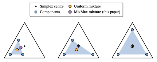
Figure 1: MixMax for classification picks the label probability that maximizes entropy (is closest to the centre of the simplex) in the convex hull of the distributions. We illustrate the label probabilities given by MixMax compared to balancing the distributions when there is only one input and the objective is to minimize worst-case cross-entropy loss.

2 Preliminaries

We work with functions $f:\mathcal{X}\to\mathcal{O}$ from an input domain $\mathcal{X}$ (with a measure $dx$) to a closed convex output domain $\mathcal{O}\subset\mathbb{R}^{n}$ that have bounded $L^{\infty}$ norm in each output coordinate: we denote this function space by $L^{\infty}(\mathcal{X},\mathcal{O})$. For example, when doing classification $\mathcal{O}$ could be the probability simplex, with the i’th entry representing the probability of label $i$. We will specifically consider the set of functions with outputs bounded by some value $r$ in every coordinate (a.e.), denoted by $B_{L^{\infty}(\mathcal{X},\mathcal{O})}(r)$. We work with data $(x,y)$ where $x\in\mathcal{X}$ and $y\in\mathcal{Y}$, and an associated loss function $\mathcal{L}(o,y):\mathcal{O}\times\mathcal{Y}\rightarrow\mathbb{R}^{+}$ that is convex in the first argument and continuous in both. An example is cross-entropy where $o$ is the label probabilities, and $y$ is a specific label. With $\mathcal{L}$ we have the expected loss of a function $f\in L^{\infty}(\mathcal{X},\mathcal{Y})$ over a distribution $dp$ on $\mathcal{X}\times\mathcal{Y}$ is $\int_{\mathcal{X}\times\mathcal{Y}}\mathcal{L}(f(x),y)dp(x,y)$. Given a set of distributions $P$, the DRO objective we study is

$$\inf_{f\in B_{L^{\infty}}(r)}\sup_{dp\in P}\int\mathcal{L}(f(x),y)dp(x,y)$$ (DRO)

3 DRO Over Bounded Functions is Solved by Data Mixing

We now show that, letting our model class be all bounded functions, fitting to an optimal data mixture returns a function that solves group DRO. This is done by observing the set of all bounded functions has a sufficient amount of regularity under the right metric. We further show that this optimal mixture is characterized by having the highest Bayes error. Later in Section 4 we demonstrate how to optimize for this mixture in the case of cross-entropy and $\ell_{2}^{2}$ loss.

Formally, Theorem 3.1 states that there exists a minimizer to the hardest distribution which solves DRO. This follows by applying Sion’s minimax theorem to the space of bounded functions, however, this requires first showing that the space of bounded functions meets the assumptions needed for Sion’s minimax theorem. For example, we will require that $dx$ is a $\sigma$-finite measure, which is satisfied if $dx$ is Lebesque measure on $R^{n}$ or counting measure on some countable set. We will further require that $\mathcal{L}$ is bounded on $\mathcal{O}\times\mathcal{Y}$ and discuss the strength of this assumption later. A complete proof is provided in Appendix A.1

Theorem 3.1 (DRO over $L^{\infty}$ = DM).

Let $P$ be a set of probability distributions $dp$ on the product space $\mathcal{X}\times\mathcal{Y}$ with $\mathcal{Y}\subset\mathbb{R}^{n}$ for some $n$, such that $\forall dp\in P$, $dp(x)$ is absolutely continuous w.r.t a given $\sigma$-finite measure $dx$ on $\mathcal{X}$. Let $\mathcal{O}\subset\mathbb{R}^{m}$ be a closed convex set, and $L^{\infty}(\mathcal{X},\mathcal{O})$ be defined w.r.t the measure $dx$, and $B_{L^{\infty}(\mathcal{X},\mathcal{O})}(r)=\{f\in L^{\infty}(\mathcal{X},\mathcal{O}):||f||_{\infty}\leq r\}$.

Let the loss function $\mathcal{L}(o,y)$ be continuous in both arguments, and convex in the first argument. Furthermore assume $\mathcal{L}$ is bounded by some constant $M$ on $\mathcal{O}\times\mathcal{Y}$. If $dp_{\lambda}$ realizes

$$\sup_{dp\in Conv(P)}\inf_{f\in B_{L^{\infty}(\mathcal{X},\mathcal{O})}(r)}\int\mathcal{L}(f(x),y)dp(x,y)$$

and there exists an $f^{*}\in B_{L^{\infty}(\mathcal{X},\mathcal{O})}(r)$ realizing the DRO objective, then there exists a minimizer $f_{\lambda}$ of the expected loss under $dp_{\lambda}$ that also realizes the DRO objective

$$\inf_{f\in B_{L^{\infty}(\mathcal{X},\mathcal{O})}(r)}\sup_{dp\in P}\int\mathcal{L}(f(x),y)dp(x,y)$$

That is, the DRO objective is solved by fitting a specific distribution in the convex hull of $P$. If the set of distributions $P$ is finite, then the DRO objective is solved by fitting a specific mixture distribution.

While bounded loss may seem strong, it can be enforced by choosing the output space $\mathcal{O}$ carefully, e.g., for cross-entropy loss if we know the minimum probability of any label is $\epsilon>0$ we can choose $\mathcal{O}$ accordingly and avoid loss blow-up (due to $log(0)$). Note, our actual requirement was a condition to enforce that pointwise convergence in the loss at every $x$ implies convergence of the integral for all $dp\in P$, which can be true without loss boundedness depending on $P$. On the assumption that a DRO solution over $B_{L^{\infty}(\mathcal{X},\mathcal{O})}(r)$ exists, this is the case for finite $P$ (Appendix A.1).

For the rest of the paper, We will assume there is sufficient regularity (whether imposed by $\mathcal{O}$, $P$, or both) for pointwise convergence of loss to imply the average loss converges and hence the result of Theorem 3.1 applies. We will further assume that for some $r<\infty$ we have the bounded functions $B_{L^{\infty}(\mathcal{X},\mathcal{O})}(r)$ contains the Bayes optimal solutions for all $dp\in P$ (to leverage structural properties of cross-entropy and $\ell_{2}^{2}$). Note the last two assumptions are satisfied for cross-entropy if a.e. all labels have $\geq\epsilon$ probability for some $\epsilon>0$ (and we choose $\mathcal{O}$ accordingly), and for $\ell_{2}^{2}$ if the allowed $y$ values are bounded. We leave it to future work to consider applying Theorem 3.1 without these assumptions, or generalizing Theorem 3.1 itself.

For cross-entropy and $\ell_{2}^{2}$ losses, the Bayes optimal functions are unique up to a measure 0 set over $\mathcal{X}$, and so any minimizer of the hardest distribution is DRO optimal 3.1 (given a DRO solution exists): all minimizers have the same average losses on $dp\in P$. In this case, we have the optimization over bounded functions reduces to optimization over a finite dimensional simplex $\Delta^{P}$ if the set $P$ is finite. This is by parameterizing $Conv(P)$ with $\lambda\in\Delta^{P}$ via ${Conv(P)=\{dp_{\lambda}\coloneqq\sum_{dp\in P}\lambda_{p}dp:\lambda\in\Delta^{P}\}}$, and denoting the unique (a.e.) minimizer of $\int\mathcal{L}(f(x),y)dp_{\lambda}(x,y)$ in $B_{L^{\infty}(\mathcal{X},\mathcal{O})}(r)$ by $f_{\lambda}$ (parameterized by $\lambda$).

Corollary 3.2.

Let $P$ be a finite set, and assume $\int\mathcal{L}(f(x),y)dp(x,y)$ is uniquely minimized over fucntions in $B_{L^{\infty}(\mathcal{X},\mathcal{O})}(r)$ (upto a measure $0$ set). Parameterize $Conv(P)$ by ${\lambda\in\Delta^{P}}$ via ${Conv(P)=\{dp_{\lambda}\coloneqq\sum_{dp\in P}\lambda_{p}dp:\lambda\in\Delta^{P}\}}$. Further denote the minimizer of $\int\mathcal{L}(f(x),y)dp_{\lambda}(x,y)$ in $B_{L^{\infty}(\mathcal{X},\mathcal{O})}(r)$ by $f_{\lambda}$ (parameterized by $\lambda$). Then for $\lambda$ realizing $\inf_{\lambda\in\Delta^{P}}\sup_{dp\in P}\int\mathcal{L}(f_{\lambda}(x),y)dp(x,y)$, $f_{\lambda}(x)$ realizes $\inf_{f\in B_{L^{\infty}(\mathcal{X},\mathcal{O})}(r)}\sup_{dp\in P}\int\mathcal{L}(f(x),y)dp(x,y)$. That is, the optimization over $L^{\infty}$ reduces to an optimization over $\Delta^{P}$.

Proof.

Follows by noting that a solution to the minmax objective is a solution to a specific mixture by Theorem 3.1 (and noting $P$ is finite so a DRO solution exists), and hence we can restrict to that space which is parameterized by $\Delta^{P}$. ∎

4 MixMax 

Algorithm 1 MixMax 

Require: Step size $\eta$, number of steps $n$, loss function $\mathcal{L}$ (either cross-entropy or $\ell_{2}^{2}$), and, for each distribution $dp$ in the set $P$, samples $D_{p}$, proxy/exact covariate density $p(x)$, and proxy/Bayes optimal function $f_{p}$.

Note: If there is no covariate shift then can set $p(x)=q(x)~{}\forall dp\in P$ for any fixed $q(x)$ and has no impact due to symmetry in the formula used in the algorithm.

Initialize: $\lambda_{p}\leftarrow\frac{1}{|P|}$ for all $dp\in P$

1:  for $i=1,\ldots,n$ do

2:     $f_{\lambda}(x)\leftarrow\frac{\sum_{p\in P}\lambda_{p}p(x)f_{p}(x)}{\sum_{p\in P}\lambda_{p}p(x)}$

3:     $l\leftarrow\sum_{dp\in P}\frac{\lambda_{p}}{|D_{p}|}\sum_{(x,y)\in D_{p}}\mathcal{L}(f_{\lambda}(x),y)$

4:     $g\leftarrow\nabla_{\lambda}l$

5:     $\lambda_{p}\leftarrow\frac{\lambda_{p}e^{\eta g_{p}}}{\sum_{dp\in P}\lambda_{p}e^{\eta g_{p}}}$ for all $dp\in P$

6:  end for

7:  return  $\{\lambda_{p}\}_{dp\in P}$

We now apply Theorem 3.1 (under the assumptions of the previous section) to cross-entropy and $\ell_{2}^{2}$ for finite $P$. We use $p(x)$ and $f_{p}(x)$ to represent the covariate density and Bayes optimal function of $dp\in P$, and $p_{\lambda}(x)$ and $f_{\lambda}(x)$ similarly for $dp_{\lambda}\in Conv(P)$.

First note that, by Theorem 3.1 and Corollary 3.2, the objective for the optimal mixture weights is

$$\sup_{\lambda\in\Delta^{P}}\int\mathcal{L}(f_{\lambda}(x),y)dp_{\lambda}(x,y)=\sup_{\lambda\in\Delta^{P}}\sum_{dp\in P}\lambda_{p}\int\mathcal{L}(f_{\lambda}(x),y)dp(x,y)$$ (1)

We show that this is concave and that we can compute its gradients for cross-entropy and $\ell_{2}^{2}$. Thus, we can perform entropic mirror ascent [12] to solve the constrained optimization. Algorithm 1 describes this approach, which we call MixMax ("Mixtures by Maximization").

The Objective is Concave

In the case of cross-entropy, under our assumptions, this objective reduces to the expected entropy of $y$ conditioned on $x$, $p_{\lambda}(y|x)$, over $p_{\lambda}(x)$. Therefore it is a concave maximization problem in the mixture weights. In the case of $\ell_{2}^{2}$, under our assumptions, this objective reduces to the expectation of the conditional variance of $y$ given $x$ over $p_{\lambda}(x)$, which is again a concave objective. Appendix A.2 provides proofs of concavity.

4.1 Idealized Gradients of the MixMax Objective

We now demonstrate how to compute the gradient of the objective in Equation 1, which is $\sum_{dp\in P}\int\nabla_{\lambda}\lambda_{p}\mathcal{L}(f_{\lambda}(x),y)dp(x,y)$ , given $f_{p}$ and $p(x)$ and the ability to integrate for all $dp\in P$. This proceeds in cases, and we later discuss how to implement this empirically.

Case 1: No Covariate Shift

Suppose there is no covariate shift, i.e., $\exists~{}p_{0}(x)$ such that $p(x)=p_{0}(x)~{}\forall dp\in P$. Then, for cross-entropy we have $f_{\lambda}(x)=\sum_{dp\in P}\lambda_{p}p(y|x)=\sum_{dp\in P}\lambda_{p}f_{p}(x)$ and for $\ell_{2}^{2}$ we have $f_{\lambda}(x)=\sum_{dp\in P}\lambda_{p}\mathbb{E}_{y\sim p(y|x)}y=\sum_{dp\in P}\lambda_{p}f_{p}(x)$. Hence given $f_{p}(x)~{}\forall dp\in P$ we can compute $f_{\lambda}(x)$ and $\nabla_{\lambda}f_{\lambda}(x)$. Computing $\nabla_{\lambda}\lambda_{p}\mathcal{L}(f_{\lambda}(x),y)$ follows by product and chain rule, and given the ability to integrate over $dp\in P$ we can compute the gradient of the objective.

Case 2: Covariate Shift

The more general expression under covariate shift, for cross-entropy and $\ell_{2}^{2}$, is $f_{\lambda}(x)=\frac{\sum_{dp\in P}\lambda_{p}f_{p}(x)p(x)}{\sum_{dp^{\prime}\in P}\lambda_{p^{\prime}}p^{\prime}(x)}$. Hence computing $f_{\lambda}(x)$ and $\nabla_{\lambda}f_{\lambda}(x)$ would further require knowledge of $p(x)~{}\forall dp\in P$. Given this, computing $\nabla_{\lambda}\lambda_{p}\mathcal{L}(f_{\lambda}(x),y)$ follows by product and chain rule, and given the ability to integrate over $dp\in P$ we can compute the gradient of the objective.

4.2 Empirical MixMax and Practical Considerations

One usually does not know the Bayes optimal function $f_{p}(x)$, nor the covariate density function $p(x)$, for all $dp\in P$. However one may be able to construct approximations $\hat{f_{p}}(x)$ and $\hat{p}(x)$ of $f_{p}(x)$ and $p(x)$ for $dp\in P$, and these can be used instead to run an approximate version of MixMax . For example, one can train a model on samples from $dp\in P$ to obtain $\hat{f_{p}}(x)$, and similarly for $\hat{p}(x)$.

Furthermore, computing the integral over $dp\in P$ exactly is also often not possible. However, given samples $D_{p}$ from each $dp\in P$, one can construct a Monte Carlo estimate of the gradient

$$\sum_{dp\in P}\int\nabla_{\lambda}\lambda_{p}\mathcal{L}(f_{\lambda}(x),y)dp(x,y)\approx\sum_{dp\in P}\frac{1}{|D_{p}|}\sum_{(x,y)\in D_{p}}\nabla_{\lambda}\lambda_{p}\mathcal{L}(f_{\lambda}(x),y)$$

This gradient estimator is used in MixMax, and is unbiased if we know the true $f_{\lambda}$. However, practically, even if we have unbiased estimates $\hat{f_{p}}(x)$ and $\hat{p}(x)$ computed with independent samples from $dp\in P$, it is not clear that plugging them into the gradient calculation in MixMax and running the Monte Carlo estimate with another set of independent samples leads to an unbiased estimator of the true MixMax objective gradients. One would want the expectation of this gradient estimate (over resampling all the datapoints used) to be the gradient using the expectations of $\hat{f_{p}}(x)$ and $\hat{p}(x)$, but instead it is the expectation of the gradient using estimates $\hat{f_{p}}(x)$ and $\hat{p}(x)$, and the expectation does not commute with the gradient function (the gradient function is non-linear for cross-entropy and $\ell_{2}^{2}$).

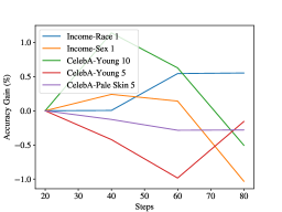
Figure 6: We see that MixMax biased by running on proxy training data can benefit from early stopping for several datasets, as seen by the peaks in performance, however these trends are statistically weak given the standard deviations reported in Table 3. Here we plot the worst group accuracy gain over running MixMax for $20$ steps when running MixMax for $20,40,60,80$ steps. Further hyperparameter details are described in Appendix B. This is done for the datasets observed to have big label shifts, described in Table 1

We ignore this issue and settle for approximate MixMax as anyways the proxy models we use are not guaranteed to be unbiased estimates of $f_{p}(x)$ and $p(x)$ (they are from more restricted model classes). However, we did empirically test whether there was an advantage to having independent samples for constructing $\hat{f_{p}}$ and running MixMax, which seemed intuitively better as test loss is different than training loss, but found reusing training samples performed comparably to having independent samples (Section 6.2). We also observed that optimizing the approximate MixMax objective defined by proxies for more steps is not always better (Figure 6 in Appendix C), however, these trends were statistically weak given the standard deviations reported in Table 3 (Appendix C).

5 Related Work

5.1 Distributionally Robust Optimization

DRO is motivated by several applications not limited to just machine learning, such as resource allocation [13]. Approaches for DRO often focus on “uncertainty" sets $P$ (the set of distributions we are minimizing the maximum error over) that admit a duality theory [24, 10, 4, 32, 3], such as Lagragian duality, conic duality, Fenchel duality, etc. For theorem 3.1 we assume nothing on $P$, and for some results, that it is finite similar to work on the Cutting-Surface approaches to DRO [24, 23, 25, 2]; the finite $P$ case is widely called Group DRO [26] in deep learning for its applications where well-specified "groups" exist in the collected data. In particular, for finite $P$ the equivalence to the convex hull of the set of distributions used in Theorem 3.1 already appears as Lemma 17 in Rahimian and Mehrotra [24] and is wide-spread in the finite $P$ literature. On similarity in theory, our main theorem that DRO is solved by data mixing is most closely related to the saddle point approaches to stochastic programming [28, 13]. These results present duality theory where solving for the hardest distribution is enough when the set of parameters to minimize w.r.t is a subset of $\mathbb{R}^{n}$. In the case of Dupačová [13] a focus is placed on sets of all distributions meeting certain moment constraints (e.g., only the mean and variance are known). Shapiro and Kleywegt [28] instead considers the case of an arbitrary finite set of distributions like our work, proposing sample average approaches for optimal solutions. Our method also uses sample averages, but further leverages the structure of cross-entropy and $\ell_{2}^{2}$ loss.

Nevertheless, to the best of our knowledge, our work is the first to extend these past minimax approaches to DRO over the set of all bounded functions (Theorem 3.1). This yields a concave objective to maximize which we find yields good results for practical applications involving non-parametric learning and expressive non-convex model classes.

5.2 Data Mixing

The work of Xie et al. [33], building on past work on DRO for deep learning [26, 22], highlighted empirically how optimizing dataset mixtures can lead to better performance over several downstream tasks. However, it is not clear whether this is due to faster convergence or due to the optima being better suited for the set of downstream tasks. On this, past work has highlighted the role of dataset selection for convergence rates [30, 20], alongside increasing sample access [19]. In this paper we asked what the role of dataset selection, in particular data mixing, is for having optima better suited for deployments with uncertain downstream tasks. We note recent work by Fan et al. [14] proposed data mixing methods that build on Xie et al. [33], but they departed away from the DRO objective (and Xie et al. [33] still performed comparably with enough compute).

6 Experiments

MixMax only has guarantees when we can obtain the optimal model over all bounded functions. This is not possible in practice. Hence, we empirically tested how it performed for real-world model classes with only finite samples from each distribution. In our experiments, we ran MixMax until its objective converged to within $0.01$ between iterates unless otherwise specified; preliminary testing showed that this happened after $10$ steps with $\eta=2.0$ for all the sequence modeling tasks, and for $20$ steps with $\eta=0.1$ for the tabular datasets. We used Nvidia RTX 2080 Ti and A100 GPUs to accelerate our experiments involving small transformers, and otherwise used Intel Xeon Silver 4210 CPUs and AMD EPYC 7643 CPUs. Our experiments with small transformers used the GPTNeo architecture  [6] with hyperparameters described in Appendix B.

6.1 Illustrating MixMax Improvements over Balancing

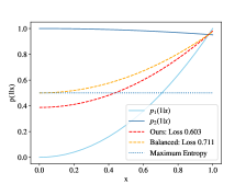
(a) Binary Classification Example

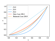
(b) Regression Example

Figure 2: Empirical MixMax provides weights different than balanced and reduced worst-distribution test loss for binary classification and $\ell_{2}^{2}$ regression.

We investigated how empirical MixMax compared to balancing data on toy tasks without proxy functions. We considered two binary classification distributions with the same covariate probabilities $p(x)=unif[0,1]$, but with $p_{1}(1|x)=x^{2}$ and $p_{2}(1|x)=|cos(0.1\pi x)|$, and three deterministic regression distributions with again the same covariate probabilities $p(x)=unif[0,1]$, but now $p_{1}(y|x)=\delta_{x}(y)$, $p_{2}(y|x)=\delta_{x^{2}}(y)$ and $p_{3}(y|x)=\delta_{x^{3}}(y)$ ($\delta$ denotes a point mass). From all distributions we sampled a train and test set, and ran MixMax with the train sets, with hyperparameters described in Appendix B. MixMax gave weights $[0.613,0.387]$ and $[0.500,0.0,0.500]$ for binary classification and regression respectively. For binary classification these weights promoted a function closer to maximum entropy on average over the domain (the objective we maximized), and for regression MixMax balanced the distributions whose Bayes optimal function were the extreme functions. In both cases MixMax reduced worst-distribution test loss, as described in Figure 2.

6.2 MixMax Performs Better than Group DRO and DoReMI for Sequence Modeling

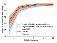
(a) Comparing mixtures found by different methods.

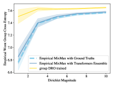
(b) Comparing group DRO Models

Figure 3: MixMax found better mixture weights on a simple sequence modeling task, and its ensemble model performed better than the group DRO trained model. The improvement is even stronger when the distributions are less similar. We present the mean and $0.5$ standard deviation of the worst group (i.e., Markov chain) cross-entropy of the Bayes optimal function defined by the different methods’ mixture weights in Figure 3(a). Figure 3(b) further compares the performance between using MixMax weights to ensemble its proxy functions and the model given by training with group DRO.

We investigated how MixMax compared to other mixture finding methods (balanced and DoReMi [33]) and the original gradient descent and ascent group DRO algorithm [26] across sets of distributions with varying similarity. Specifically, we considered 4 tokens $\{0,1,2,3\}$ and sequences generated by a Markov chain, and the task was to model the mixed distribution of sequences from lengths $1$ to $10$ where the probability a sequence was of length $i$ was always $1/10$. We constructed three Markov chains to perform group DRO over by independently sampling transition probabilities from a symmetric Dirichlet distribution, with magnitudes $1.0,3.0,5.0,7.0,10.0$ representing increasing similarity between the Markov chains. For all methods we took a training set of $800$ samples per length and a test set of $200$ samples per length from each Markov chain. We applied MixMax given both the true probabilities and a small transformer trained for next token prediction on $600$ of the $800$ training samples per length (leaving the other $200$ training samples per length to run MixMax). We applied DoReMi and group DRO using the same small transformer architecture and all $800$ training samples per length (per Markov chain). Hyperparameters are described in Appendix B, and we reported the results for each method with the hyperparameter settings that had the lowest maximum group cross-entropy test set loss over $15$ trials of generating sets of Markov chains and samples.

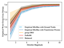
(a) Optimally Fitting Mixture

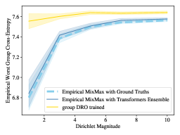
(b) Empirically Fitting Mixture

Figure 5: A reproduction of the experimental setup for Figure 5 but with fewer training samples ($500$ instead of $800$) We still see that a model (empirically by ensembling transformers or optimally) to MixMax mixture weights performs better than DoReMi and group DRO mixture weights, and the model trained by group DRO. Furthermore, we still see that the improvement is even stronger when the distributions are less similar.

We found MixMax returned better mixtures to fit to than other methods, and that ensembling its proxy transformers with its mixture weights performed better than training with group DRO. Specifically, in Figure 3(a) we compared the worst group cross-entropy loss of the Bayes optimal function for the mixture given by MixMax using transformers for proxy (and ground truths as a baseline), DoReMi, the average group DRO mixture weights, and also balanced weights. As seen, fitting to the mixture given by MixMax always performed best, doing even better as the distributions became less similar (lower magnitude). We also found the mixture weights returned by group DRO performed comparably to balanced, consistent with previous findings on group DRO performance [18]. However, we note that group DRO’s intended use is to apply the model it trained and not its mixture weights. In Figure 3(b) we observed using MixMax mixture weights (obtained using transformers for proxies) to ensemble its proxy models performed better than the group DRO trained model; note the methods have comparable training compute as the $3$ models in the ensemble trained on $1/3$ of the training set each. These results were consistent even if we used fewer training samples (Figures 5(b) 5(a) in Appendix C) highlighting that we had sufficient samples for both experiments.

Reusing Training Samples is Comparable

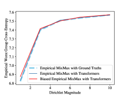
(a) $800$ Training Samples

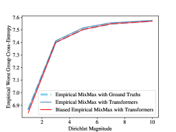
(b) $500$ Training Samples

Figure 7: Reusing the proxy training points for MixMax is not much worse than using seperate data, and can be slightly better when one has fewer training samples. Here we consider the experimental setup from Figure 3(a) for fitting MixMax mixture weights optimally, and present results for when the same $800$ or $500$ training points are used to fit the proxy models and run MixMax (instead of the $600-200$ and $300-200$ split for proxy training and MixMax).

Figure 7 (in Appendix C) shows that reusing the proxy models training data to run MixMax performed comparably to having independent sets. This suggests one can effectively reuse training samples to run MixMax and be more sample efficient.

6.3 MixMax Beats Balancing Data for XGBoost

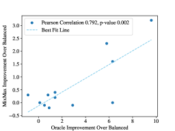
Figure 4: Empirical MixMax improved worst group accuracy over balancing data more when there was bigger room for improvement. We plot the improvement in worst group accuracy from training on MixMax mixture weights over balanced data as a function of the Oracle worst group accuracy (i.e., having a model trained for each distribution) improvement over balanced data. The points are from the different settings in Table 1. We observed a Pearson correlation of $0.792$ with p-value $0.002$.

Datasets	Features	Oracle ($\%$)	Balanced ($\%$)	MixMax ($\%$)
Inc-Race	All	$79.1(\pm 1.2)$	$80.0(\pm 1.2)$	$80.3(\pm 0.6)$
	$2$	$71.2(\pm 0.1)$	$70.7(\pm 0.2)$	$70.6(\pm 0.3)$
	$1$	$60.0(\pm 0.1)$	$53.7(\pm 0.4)$	$53.7(\pm 0.5)$
Inc-Sex	All	$81.2(\pm 0.1)$	$81.1(\pm 0.2)$	$81.1(\pm 0.1)$
	$2$	$72.8(\pm 0.1)$	$71.4(\pm 0.2)$	$71.6(\pm 0.1)$
	$1$	$62.8(\pm 0.2)$	$56.5(\pm 0.2)$	$\mathbf{58.1(\pm 1.8)}$
CelebA-Young	All	$77.0(\pm 0.1)$	$75.6(\pm 0.2)$	$\mathbf{76.0(\pm 1.0)}$
	$10$	$68.3(\pm 0.3)$	$62.5(\pm 0.3)$	$\mathbf{64.8(\pm 1.6)}$
	$5$	$63.4(\pm 0.3)$	$53.8(\pm 0.2)$	$\mathbf{57.0(\pm 0.6)}$
CelebA-Pale Skin	All	$78.2(\pm 0.3)$	$77.3(\pm 0.2)$	$77.1(\pm 0.6)$
	$10$	$67.6(\pm 0.1)$	$66.8(\pm 0.2)$	$\mathbf{67.1(\pm 0.3)}$
	$5$	$62.4(\pm 0.2)$	$59.5(\pm 0.3)$	$59.4(\pm 0.3)$

Table 1: MixMax improved worst group accuracy over the baseline of balancing data for tabular dataset using XGBoost, in particular when more significant label shifts were present (see Figure 4 for a visualization). We present the average minimum accuracy over the groups from $5$ trials with random training-test splits for MixMax , even balancing by up-sampling, and the "oracle" accuracy where a model was trained for each group and is evaluated on the same group (as an example of optimal performance). Results are bolded if the better method’s average performance was outside one standard deviation of the other method. We modified the datasets to study a variety of shifts by only including the first $N$ features.

We compared empirical MixMax weights to data balancing for non-parametric learning algorithms, in particular XGBoost [9] known to be the state of the art for tabular data. We selected ACSIncome [11] (released under the MIT license) and CelebA annotations [21] (released for non-commercial use ) to test on. For ACSIncome we constructed the dataset from the first $10$ American states in alphabetic order, and considered group shifts from race and sex. We further constructed variations of the dataset using all the features, the first $2$ features, and the first feature to introduce varying covariate shifts. For CelebA annotations, we used attractiveness as the label with Young and Pale Skin as the group shifts, and constructed variations of the dataset using all features, the first $10$ features, and the first $5$ features . We used random $80\%-20\%$ train-test splits in all settings. We applied MixMax by using XGBoost models (trained on the group data) as proxies for label probabilities, and modeled covariate probabilities using Gaussian kernel density estimation. We reused the proxy training data for MixMax, and returned the XGBoost model trained on the same training data but up-sampled according to weights returned by MixMax. For the balanced baseline, we returned an XGBoost model trained with the data balanced by up-sampling the smaller groups. Lastly, as a measure for best possible performance, we also presented the worst oracle accuracy, where oracle accuracy refers to the test accuracy of an XGBoost model trained on the same distribution and given access to the group identity at test time. Hyperparameters are described in Appendix B, and we reported the results for the hyperparameter setting with the best performance over $5$ trials with random train-test splits.

As seen in Table 1, MixMax matched or outperformed the worst group accuracy of data balancing in all settings. This was also true for worst group loss (Table 2 in Appendix C). In particular, as seen in Figure 4 we observed the improvement over the worst group accuracy of data balancing was stronger when more room for improvement was possible (a larger gap between oracle and balanced worst group accuracy): we observed a $0.79$ Pearson correlation factor. In the end, we found MixMax improved the worst group accuracy of ACSIncome with groups by sex and just one feature by $1.6\%$ (relative gain of $2.8\%$), and for CelebA with groups by Young and 10 and 5 features by $2.3\%$ and $3.2\%$ (relative gains of $3.7\%$ and $5.9\%$ respectively).

7 Conclusion

In this paper we showed that group DRO over bounded functions can be solved by fitting to an optimal data mixture, and that maximizing a particular concave objective returns the optimal mixture weights for cross-entropy and $\ell_{2}^{2}$ loss. We called this method for finding data mixtures MixMax. Our experiment on a simple sequence modeling task showed that MixMax improved over previous parametric group DRO baselines. MixMax was also shown to improve over the baseline of balancing data for non-parametric learning algorithms, specifically XGBoost, for which no previous group DRO methods were proposed. We leave open the problem of applying our minimax theorem to other losses, and developing principled ways of computing the proxy models needed to run MixMax.

Limitations

A main technical limitation of MixMax is the need to model covariate shifts (if covariate shifts can exist). This may prove problematic for higher-dimensional data, which we leave for future work. Further work is also needed to investigate how generalizable our abstraction to all bounded functions is for common models beyond XGBoost and small transformers. Lastly, we acknowledge that DRO may be used to claim a model is fair, despite it still carrying societal biases. We hope future uses will take care in considering the claims DRO can and cannot make.

Appendix

Appendix A Proofs

A.1 Proof of Theorem 3.1

Proof.

First note $\sup_{dp\in P}=\sup_{dp\in Conv(P)}$ as the objective is linear in $dp$. Now note we can apply Sion’s minimax theorem [29] if $B_{L^{\infty}(\mathcal{X},\mathcal{O})}(r)$ is compact in a topology that the objective is continuous in. Note $B_{L^{\infty}(\mathcal{X},\mathbb{R}^{m})}(r)$ is compact in the Weak*-topology on $L^{\infty}(\mathcal{X},\mathbb{R}^{m})$ (as the dual of $L^{1}(\mathcal{X},\mathbb{R}^{m})$) by Banach-Alaoglu’s theorem and continuity of dilation [15]. Now note $B_{L^{\infty}(\mathcal{X},\mathcal{O})}(r)$ is a closed subset of $B_{L^{\infty}(\mathcal{X},\mathbb{R}^{m})}(r)$ and hence is also compact. The fact $B_{L^{\infty}(\mathcal{X},\mathcal{O})}(r)$ is closed follows from $\mathcal{O}$ being closed and that weak* convergence implies pointwise convergence (a.e.) in $B_{L^{\infty}(\mathcal{X},\mathbb{R}^{m})}(r)$ (a set containing $B_{L^{\infty}(\mathcal{X},\mathcal{O})}(r)$), which is proven below.

Note convergence in weak* for functions in $B_{L^{\infty}(\mathcal{X},\mathbb{R}^{m})}(r)$ means the functions converge pointwise a.e. This is as, for $g\in L^{1}$ and $f$ the limit of $f_{n}$ in the weak*-topology, $0=\lim_{n\rightarrow\infty}\int(f-f_{n})gdx=\int\lim_{n\rightarrow\infty}(f-f_{n})gdx$ by dominated convergence as functions are bounded. Now taking $g=sign(\lim_{n\rightarrow\infty}(f-f_{n}))\chi_{E}$ implies by proposition 2.16 in [15] that $\lim_{n\rightarrow\infty}(f-f_{n})(x)=0$ a.e on $E$ for finite measure sets $E$. As the space is countably coverable by finite measured sets (by the $\sigma$-finite assumption), this implies the functions converge pointwise a.e.

Now as $\mathcal{L}$ is bounded, and the functions converge pointwise in the weak*-topology, we also have by the dominated convergence theorem the objective is continuous in the weak* topology on $L^{\infty}$.

Thus we satisfy the conditions for Sion’s minimax theorem, which implies

$$\sup_{dp\in Conv(P)}\inf_{f\in B_{L^{\infty}(\mathcal{X},\mathcal{O})}(r)}\int\mathcal{L}(f(x),y)p(x,y)=\inf_{f\in B_{L^{\infty}(\mathcal{X},\mathcal{O})}(r)}\sup_{dp\in Conv(P)}\int\mathcal{L}(f(x),y)p(x,y)$$

So if $f^{*}$ achieves the inf in the RHS and $dp_{\lambda}$ achieves the sup in the RHS, then note

$$\int\mathcal{L}(f^{*}(x),y)dp_{\lambda}(x,y)\leq\sup_{dp\in Conv(P)}\int\mathcal{L}(f^{*}(x),y)dp(x,y)=\inf_{f\in B_{L^{\infty}(\mathcal{X},\mathcal{O})}(r)}\int\mathcal{L}(f(x),y)dp_{\lambda}(x,y)$$

conclude that $\int\mathcal{L}(f^{*}(x),y)dp_{\lambda}(x,y)=\inf_{f\in B_{L^{\infty}(\mathcal{X},\mathcal{O})}(r)}\int\mathcal{L}(f(x),y)dp_{\lambda}(x,y)$. So in particular $f^{*}$ is a minimizer of $dp_{\lambda}$. Note minimizers of $dp_{\lambda}$ exist by the compactness of $B_{L^{\infty}(\mathcal{X},\mathbb{R}^{m})}(r)$ and continuity of the objective over this function space.

∎

Remark on Existence of DRO Solution

The theorem required that there exists a DRO solution in the first place, and this is satisfied if $P$ is finite by the continuity of the supremum over a finite set of continuous functions (note continuity of the objective for a single $dp$ was proven above). Further care is needed when $P$ is not finite, but the paper focuses on the finite $P$ case and so we do not discuss this further.

A.2 Concavity of Objectives

Fact A.1.

If $\mathcal{L}$ is cross-entropy, then $\int\mathcal{L}(f_{\lambda}(x),y)dp_{\lambda}(x,y)$ is concave in $\lambda$.

Proof.

We note ${f_{\lambda}=p_{\lambda}(y|x)=\sum_{dp\in P}\lambda_{p}(x)p(y|x)}$ where ${\lambda_{p}(x)=\frac{\lambda_{p}p(x)}{\sum_{dp^{\prime}\in P}\lambda_{p^{\prime}}p^{\prime}(x)}=\frac{\lambda_{p}p(x)}{p_{\lambda}(x)}}$. Note that ${-\int_{\mathcal{Y}}\log(\sum_{dp\in P}\lambda_{p}(x)p(y|x))\sum_{dp\in P}\lambda_{p}(x)p(y|x)\geq\sum_{dp\in{}}\lambda_{p}(x)\int_{\mathcal{Y}}-log(p(y|x))p(y|x)}$ by the concavity of entropy. Applying this we have

$$\int_{\mathcal{X}}\int_{\mathcal{Y}}-log(p_{\lambda}(y|x))p_{\lambda}(y|x)p_{\lambda}(x)\\ \geq\int_{\mathcal{X}}\left(\sum_{dp\in P}\lambda_{p}(x)\int_{\mathcal{Y}}-log(p(y|x))p(y|x)\right)p_{\lambda}(x)\\ =\int_{\mathcal{X}}\left(\sum_{dp\in P}\frac{\lambda_{p}p(x)}{p_{\lambda}(x)}\int_{\mathcal{Y}}-log(p(y|x))p(y|x)\right)p_{\lambda}(x)\\ =\sum_{dp\in P}\lambda_{p}\int_{\mathcal{X}}\int_{\mathcal{Y}}-log(p(y|x))p(y|x)p(x)$$ (2)

this proves concavity w.r.t $\lambda$, as desired.

∎

Fact A.2.

If $\mathcal{L}$ is $\ell_{2}^{2}$, then $\int\mathcal{L}(f_{\lambda}(x),y)p_{\lambda}(x,y)$ is concave in $\lambda$

Proof.

We assume $f_{\lambda}$ is the bayes optimal solution, hence we have the loss is the bayes error $\int_{\mathcal{X}}Var_{p_{\lambda}(y|x)}(y|x)p_{\lambda}(x)$. Note $p_{\lambda}(y|x)=\sum_{dp\in P}\lambda_{p}(x)p(y|x)$ where $\lambda_{p}(x)=\frac{\lambda_{p}p(x)}{\sum_{dp^{\prime}\in P}\lambda_{p^{\prime}}p^{\prime}(x)}=\frac{\lambda_{p}p(x)}{p_{\lambda}(x)}$, and variance is concave w.r.t mixture weights. Thus we have

$$\int\mathcal{L}(f_{\lambda}(x),y)p_{\lambda}(x,y)\\ =\int_{\mathcal{X}}Var_{p_{\lambda}(y|x)}(y|x)p_{\lambda}(x)\\ \geq\int_{\mathcal{X}}\left(\sum_{dp\in P}\lambda_{p}(x)Var_{p(y|x)}(y|x)\right)p_{\lambda}(x)\\ =\int_{\mathcal{X}}\left(\sum_{dp\in P}\frac{\lambda_{p}p(x)}{p_{\lambda}(x)}Var_{p(y|x)}(y|x)\right)p_{\lambda}(x)\\ =\sum_{dp\in P}\lambda_{p}\int_{\mathcal{X}}Var_{p(y|x)}(y|x)p(x)\\ =\sum_{dp\in P}\lambda_{p}\int\mathcal{L}(f_{p}(x),y)p(x,y)$$ (3)

This proves concavity ∎

Appendix B Experimental Setups

B.1 Toy Experiments

For the binary classification task, We ran MixMax with $D_{i}$ consisting of $10000$ samples from each distribution, step size $\eta=0.5$, and for $100$ steps. We evaluated the worst distribution cross-entropy loss by sampling another $10000$ points from each distribution.

We ran MixMax with $D_{i}$ again consisting of $10000$ samples from each distribution, and $\eta=0.001$ for $100$ steps. We then evaluated the worst $\ell_{2}^{2}$ loss by sampling another $10000$ points from each distribution.

B.2 Sequence Modeling

For MixMax , letting $y$ denote a sequence, note the task was to model $p(y)$ and so had no covariates and hence had no covariate shift (as one can take $\mathcal{X}$ to be a singleton). Thus MixMax only needed functions for the token probabilities from each distribution, and we considered both the true probabilities (as the optimal baseline) and transformers trained on each Markov chain as the proxy optimal functions. The transformer used is GPTNeo [6] with $6$ hidden states, $2$ hidden layers, $2$ attention heads, $8$ intermediate size, and with $12$ max position embeddings. In both cases we used $200$ samples per length to run MixMax , keeping the other $600$ to train the proxy model. The proxy model is trained for $20$ epochs using AdamW with learning rates $0.01,0.001$ and $0.0001$ (and otherwise default Pytorch hyperparameters).

We implemented DoReMi for finding mixture weights using the same transformer architecture as above, with the reference model being trained on a balanced dataset. The DoReMi reference and proxy models were again trained for $20$ epochs using AdamW with learning rate $0.01,0.001$ and $0.0001$ (and otherwise default Pytorch hyperparameters). The learning rate for the mixture weights was $0.1$. We also implemented group DRO with the same architecture, with the same model weights optimizer and mixture weights learning rate $0.1$. Furthermore, we tested varying minibatch sizes for the training of all models ($50,100,200$), and number of steps used for group DRO ($150,300,600$). In Figure 3 we reported the results for the hyperparameter settings with the lowest mean error for each method over $15$ trials of randomly generating markov chains according to the varying magnitudes.

B.3 Tabular Data

For running Gaussian kernel density estimation, we used the Scott method for bandwidth selection [27]. For fitting the model on MixMax mixture weights, the reference models used for MixMax on the Income dataset, and the baseline of balancing the dataset, we implemented XGBoost with depths $6,8,10$, number of trees $100,200,300$, and learning rates $0.01,0.1$ and reported the results for the hyperparameter setting with the best average accuracy over $5$ trials with random train-test splits. For CelebA, the oracle accuracies and the reference models used in MixMax were always trained used depth $8$, number of trees $200$, and learning rate $0.1$; we found hyperparameter sweeping the models on individual groups had marginal impact, and anyways would only improve our results (the baseline of balancing always has a hyperparameter sweep).

Appendix C Additional Tables and Figures

Datasets	Features	Balanced	MixMax
Inc-Race	All	$0.426(\pm 0.013)$	$0.422(\pm 0.007)$
	$2$	$0.557(\pm 0.001)$	$0.559(\pm 0.003)$
	$1$	$0.707(\pm 0.004)$	$\mathbf{0.688(\pm 0.020)}$
Inc-Sex	All	$0.403(\pm 0.004)$	$0.405(\pm 0.005)$
	$2$	$0.544(\pm 0.002)$	$\mathbf{0.541(\pm 0.006)}$
	$1$	$0.616(\pm 0.001)$	$\mathbf{0.611(\pm 0.003)}$
CelebA-Young	All	$0.495(\pm 0.002)$	$\mathbf{0.488(\pm 0.015)}$
	$10$	$0.644(\pm 0.002)$	$\mathbf{0.614(\pm 0.019)}$
	$5$	$0.706(\pm 0.002)$	$\mathbf{0.670(\pm 0.007)}$
CelebA-Pale Skin	All	$0.465(\pm 0.001)$	$0.468(\pm 0.006)$
	$10$	$0.594(\pm 0.001)$	$\mathbf{0.588(\pm 0.005)}$
	$5$	$0.647(\pm 0.001)$	$\mathbf{0.641(\pm 0.005)}$

Table 2: MixMax improved worst group loss over the baseline of balancing data for tabular dataset using XGBoost. We present the average maximum loss over the groups from $5$ trials with random training-test splits for MixMax and even balancing by up-sampling. Results are bolded if the better method’s average performance was outside one standard deviation of the other method. We modified the datasets to study a variety of shifts by only including the first $N$ features.

Dataset	Features	Untuned MixMax	Tuned MixMax
Inc-Race	$1$	$53.7(\pm 0.5\%)$	$\mathbf{54.3(\pm 0.6\%)}$
Inc-Sex	$1$	$58.1(\pm 1.8\%)$	$58.4(\pm 1.8\%)$
CelebA-Young	$10$	$64.8\%(\pm 1.6\%)$	$66.0\%(\pm 2.1\%)$
	$5$	$57.0\%(\pm 0.6\%)$	$57.0\%(\pm 0.6\%)$
CelebA-Pale Skin	$5$	$59.4\%(\pm 0.3\%)$	$59.4\%(\pm 0.3\%)$

Table 3: Empirical MixMax can sometimes be improved by doing a hyperparameter search over MixMax number of steps ($20,40,60,80$). We present the settings from Table 1 where the gap between oracle accuracy and the balanced accuracy was more than $2\%$, and include the average minimum accuracy over groups over $5$ trials of MixMax with further hyperparameter tuning. We bolded results where the tuned performance was outside one standard deviation of untuned.

References

- Albalak et al. [2024] A. Albalak, Y. Elazar, S. M. Xie, S. Longpre, N. Lambert, X. Wang, N. Muennighoff, B. Hou, L. Pan, H. Jeong, et al. A survey on data selection for language models. arXiv preprint arXiv:2402.16827, 2024.
- Bansal et al. [2018] M. Bansal, K.-L. Huang, and S. Mehrotra. Decomposition algorithms for two-stage distributionally robust mixed binary programs. SIAM Journal on Optimization, 28(3):2360–2383, 2018.
- Ben-Tal et al. [2013] A. Ben-Tal, D. Den Hertog, A. De Waegenaere, B. Melenberg, and G. Rennen. Robust solutions of optimization problems affected by uncertain probabilities. Management Science, 59(2):341–357, 2013.
- Bertsimas et al. [2010] D. Bertsimas, X. V. Doan, K. Natarajan, and C.-P. Teo. Models for minimax stochastic linear optimization problems with risk aversion. Mathematics of Operations Research, 35(3):580–602, 2010.
- Bi et al. [2024] X. Bi, D. Chen, G. Chen, S. Chen, D. Dai, C. Deng, H. Ding, K. Dong, Q. Du, Z. Fu, et al. Deepseek llm: Scaling open-source language models with longtermism. arXiv preprint arXiv:2401.02954, 2024.
- Black et al. [2021] S. Black, L. Gao, P. Wang, C. Leahy, and S. Biderman. GPT-Neo: Large Scale Autoregressive Language Modeling with Mesh-Tensorflow, Mar. 2021. URL https://doi.org/10.5281/zenodo.5297715. If you use this software, please cite it using these metadata.
- Blackard [1998] J. Blackard. Covertype. UCI Machine Learning Repository, 1998. DOI: https://doi.org/10.24432/C50K5N.
- Chen and Paschalidis [2019] R. Chen and I. Paschalidis. Selecting optimal decisions via distributionally robust nearest-neighbor regression. Advances in Neural Information Processing Systems, 32, 2019.
- Chen and Guestrin [2016] T. Chen and C. Guestrin. Xgboost: A scalable tree boosting system. In Proceedings of the 22nd acm sigkdd international conference on knowledge discovery and data mining, pages 785–794, 2016.
- Delage and Ye [2010] E. Delage and Y. Ye. Distributionally robust optimization under moment uncertainty with application to data-driven problems. Operations research, 58(3):595–612, 2010.
- Ding et al. [2021] F. Ding, M. Hardt, J. Miller, and L. Schmidt. Retiring adult: New datasets for fair machine learning. Advances in neural information processing systems, 34:6478–6490, 2021.
- Duchi [2018] J. C. Duchi. Introductory lectures on stochastic optimization. The mathematics of data, 25:99–186, 2018.
- Dupačová [1987] J. Dupačová. The minimax approach to stochastic programming and an illustrative application. Stochastics: An International Journal of Probability and Stochastic Processes, 20(1):73–88, 1987.
- Fan et al. [2023] S. Fan, M. Pagliardini, and M. Jaggi. Doge: Domain reweighting with generalization estimation. arXiv preprint arXiv:2310.15393, 2023.
- Folland [1999] G. B. Folland. Real analysis: modern techniques and their applications, volume 40. John Wiley & Sons, 1999.
- Friedman [2001] J. H. Friedman. Greedy function approximation: a gradient boosting machine. Annals of statistics, pages 1189–1232, 2001.
- Gao et al. [2020] L. Gao, S. Biderman, S. Black, L. Golding, T. Hoppe, C. Foster, J. Phang, H. He, A. Thite, N. Nabeshima, et al. The pile: An 800gb dataset of diverse text for language modeling. arXiv preprint arXiv:2101.00027, 2020.
- Idrissi et al. [2022] B. Y. Idrissi, M. Arjovsky, M. Pezeshki, and D. Lopez-Paz. Simple data balancing achieves competitive worst-group-accuracy. In Conference on Causal Learning and Reasoning, pages 336–351. PMLR, 2022.
- Jain et al. [2024] A. Jain, A. Montanari, and E. Sasoglu. Scaling laws for learning with real and surrogate data. arXiv preprint arXiv:2402.04376, 2024.
- Kolossov et al. [2023] G. Kolossov, A. Montanari, and P. Tandon. Towards a statistical theory of data selection under weak supervision. arXiv preprint arXiv:2309.14563, 2023.
- Liu et al. [2015] Z. Liu, P. Luo, X. Wang, and X. Tang. Deep learning face attributes in the wild. In Proceedings of International Conference on Computer Vision (ICCV), December 2015.
- Oren et al. [2019] Y. Oren, S. Sagawa, T. B. Hashimoto, and P. Liang. Distributionally robust language modeling. arXiv preprint arXiv:1909.02060, 2019.
- Pflug and Wozabal [2007] G. Pflug and D. Wozabal. Ambiguity in portfolio selection. Quantitative Finance, 7(4):435–442, 2007.
- Rahimian and Mehrotra [2019] H. Rahimian and S. Mehrotra. Distributionally robust optimization: A review. arXiv preprint arXiv:1908.05659, 2019.
- Rahimian et al. [2019] H. Rahimian, G. Bayraksan, and T. Homem-de Mello. Identifying effective scenarios in distributionally robust stochastic programs with total variation distance. Mathematical Programming, 173(1):393–430, 2019.
- Sagawa et al. [2019] S. Sagawa, P. W. Koh, T. B. Hashimoto, and P. Liang. Distributionally robust neural networks for group shifts: On the importance of regularization for worst-case generalization. arXiv preprint arXiv:1911.08731, 2019.
- Scott [1979] D. W. Scott. On optimal and data-based histograms. Biometrika, 66(3):605–610, 1979.
- Shapiro and Kleywegt [2002] A. Shapiro and A. Kleywegt. Minimax analysis of stochastic problems. Optimization Methods and Software, 17(3):523–542, 2002.
- Sion [1958] M. Sion. On general minimax theorems. 1958.
- Sorscher et al. [2022] B. Sorscher, R. Geirhos, S. Shekhar, S. Ganguli, and A. Morcos. Beyond neural scaling laws: beating power law scaling via data pruning. Advances in Neural Information Processing Systems, 35:19523–19536, 2022.
- Strack et al. [2014] B. Strack, J. P. DeShazo, C. Gennings, J. L. Olmo, S. Ventura, K. J. Cios, J. N. Clore, et al. Impact of hba1c measurement on hospital readmission rates: analysis of 70,000 clinical database patient records. BioMed research international, 2014, 2014.
- Wiesemann et al. [2013] W. Wiesemann, D. Kuhn, and B. Rustem. Robust markov decision processes. Mathematics of Operations Research, 38(1):153–183, 2013.
- Xie et al. [2024] S. M. Xie, H. Pham, X. Dong, N. Du, H. Liu, Y. Lu, P. S. Liang, Q. V. Le, T. Ma, and A. W. Yu. Doremi: Optimizing data mixtures speeds up language model pretraining. Advances in Neural Information Processing Systems, 36, 2024.