Verification of entangled states under noisy measurements

Abstract

Entanglement plays an indispensable role in numerous quantum information and quantum computation tasks, underscoring the need for efficiently verifying entangled states. In recent years, quantum state verification has received increasing attention, yet the challenge of addressing noise effects in implementing this approach remains unsolved. In this work, we provide a systematic assessment of the performance of quantum state verification protocols in the presence of measurement noise. Based on the analysis, a necessary and sufficient condition is provided to uniquely identify the target state under noisy measurements. Moreover, we propose a symmetric hypothesis testing verification algorithm with noisy measurements. Subsequently, using a noisy nonadaptive verification strategy of GHZ and stabilizer states, the noise effects on the verification efficiency are illustrated. From both analytical and numerical perspectives, we demonstrate that the noisy verification protocol exhibits a negative quadratic relationship between the sample complexity and the infidelity. Our method can be easily applied to real experimental settings, thereby demonstrating its promising prospects.

I Introduction

The concept of quantum entanglement takes a central position in the field of quantum physics, representing a fundamental feature that sets it apart from its classical counterpart [1]. The existence of entanglement enables the quantum realm to address specific challenges more efficiently than classical computation [2]. The significance of entanglement is underscored by its wide contribution in numerous notable achievements within the field of quantum information theory. It plays a pivotal role in various applications, including quantum communication [3, 4, 5, 6], quantum key distribution [7, 8, 9], quantum teleportation [10, 11], superdense coding [12, 13], quantum fault-tolerant computation [14, 15, 16], and quantum algorithms such as Grover’s search algorithm [17] and Shor’s algorithm [18]. Additionally, it also assumes a crucial role in quantum error correction [19, 20, 21, 22, 23], an indispensable component of quantum computation and information theory.

Given the indispensable role of entanglement in various tasks, the precise preparation of entangled quantum states has great significance. Hence, there is a compelling need to achieve high-precision verification of quantum states one has prepared. Conventional characterization methods, such as quantum state tomography (QST) [24, 25, 26], are highly resource intensive and time consuming. Alternative methods, like direct fidelity estimation [27, 28], attain an improvement in sample complexity as compared to QST, yet still exhibit standard quantum scaling with the infidelity. Recently, quantum state verification (QSV) [29] has gained much attention for providing a resource efficient approach. QSV relies solely on local measurements and classical communication, which renders it operationally convenient in experiments. Furthermore, it is crucial to emphasize that QSV is able to achieve the Heisenberg scaling in sample complexity, rather than the standard quantum limit. This renders it significantly more efficient as compared to other characterization methods.

Up to now, a number of efficient verification protocols for various entangled states have been developed, encompassing arbitrary bipartite pure states [30], Dicke states [31], phased Dicke states [32], hypergraph states [33], etc. Some of these verification protocols, such as those for bipartite pure states [34], Greenberger-Horne-Zeilinger (GHZ) states [35] and stabilizer states [36] have even been proven to be optimal in sample complexity. The verification of quantum states has also been investigated in the adversarial scenario, a context that plays an important role in various tasks including blind measurement-based quantum computation and quantum networks [37, 38, 39]. In addition to the consideration for discrete-variable states, there have also been developments in continuous-variable state verification. These protocols have practical applications in quantum communication and quantum sensing [40]. By employing quantum nondemolition measurements, it becomes possible to enhance the sample complexity of verification protocols to the optimal global level. This approach also offers practical advantages, making it more favorable for implementation in actual experiments [41].

Not solely limited to quantum state characterization, the QSV techniques can also be effectively utilized for the purpose of quantum process verification. This includes the verification not only of standard quantum gates but also of more general quantum processes [42, 43]. It is noteworthy that this method demonstrates superior applicability as compared to the conventional technique of random benchmarking [42].

However, in the noisy intermediate-scale quantum (NISQ) era [44], local measurements used in these verification protocols are imperfect. The inclusion of measurement noise within the framework of quantum verification tasks remains an unresolved problem. Most experiments [45, 46, 47] do not account for the presence of measurement noise. This neglect leads to possible issues in the statistical analysis of the sample complexity, which plays a vital role within the QSV framework. In Ref. [48] it assumes that QSV under noisy measurements will incur type I errors, meaning that there is a probability to reject the target state. Additionally, it provides a semidefinite programming (SDP) approach for certification. However, it does not clarify how measurement noise influences the type I error rate nor the extent to which sample complexity is affected due to measurement noise.

In this work, we first conduct a systematic analysis of the impact of measurement noise on verification protocols in Sec. II. Subsequently, a necessary and sufficient condition is provided for a noisy strategy to uniquely identify the target state. In Sec. III, we focus on symmetric testing when considering sample complexity, wherein a negative quadratic relationship between sample complexity and infidelity in this particular scenario is demonstrated. Then, starting with nonadaptive verification protocols for GHZ and stabilizer states, we specifically elucidate how measurement noise influences the efficiency of the verification protocols in Sec. IV. Next, $W$ state is considered as an example when the aforementioned conditions cannot be met, then in Sec. V a SDP approach is proposed to determine whether the noisy strategy is still feasible. Finally, we conclude in Sec. VI.

II Basic Framework

The fundamental objective of QSV is to establish a well-designed protocol for verifying whether an unknown quantum state $\rho$ is the target state $|\psi\rangle$ or some bad states with the condition that $\text{$\langle\psi|$}\rho\text{$|\psi\rangle$}\leq 1-\epsilon$ [29]. In a basic verification protocol, we measure copies of $\rho$ with an ensemble of two-outcome local projective measurements $\{\Omega_{i},\mathbbm{1}-\Omega_{i}\}$ equipped with a probability distribution $\{p_{i}\}$. The corresponding verification strategy is denoted as $\Omega=\sum_{i}p_{i}\Omega_{i}$. In each measurement, if $\Omega_{i}$ occurs the state “passes”, otherwise the verification “fails”. If $\rho$ is the target state $|\psi\rangle$, we require that it always passes, that is $\forall i$, $\Omega_{i}\text{$|\psi\rangle$}=\text{$|\psi\rangle$}$. If the copies pass consecutively many times, then the verification protocol ascertains that $\rho$ is the target state with a certain confidence level.

In the worst-case scenario, the maximal probability that a bad state will pass the strategy $\Omega$ is [29]

$$\max_{\text{{\hbox{ \langle\psi | }}}\rho\text{{\hbox{ | \psi \rangle}}}\leq 1-\epsilon}\mathrm{Tr}(\Omega\rho)=1-\nu(\Omega)\epsilon\,,$$ (1)

where $\nu(\Omega)=1-\lambda_{1}$ is the spectral gap of strategy $\Omega$ between the largest eigenvalue $1$ and the second-largest eigenvalue $\lambda_{1}$. The worst-case probability for a bad state to pass the strategy $N$ times is $\left[1-\nu(\Omega)\epsilon\right]^{N}$. Thus, to achieve a confidence level $1-\delta$, the sample complexity $N$ satisfies

$$N\geq\frac{\ln\delta^{-1}}{\ln([1-v(\Omega)\epsilon]^{-1})}\approx\frac{1}{v(\Omega)}\epsilon^{-1}\ln\delta^{-1}\,.$$ (2)

In standard QSV protocols, we ignore the presence of measurement noise, which is undoubtedly inconsistent with realistic scenarios. Here by the inclusion of measurement noise, we investigate when it is still possible to distinguish the null hypothesis $\mathcal{H}_{0}$ that $\rho$ is the target state $|\psi\rangle$ from the alternative hypothesis $\mathcal{H}_{1}$ that $\rho$ is a bad state. Specifically, we consider the distinguishable conditions:

1. $\Omega\text{$|\psi\rangle$}=\lambda_{0}\text{$|\psi\rangle$}$ , with $\lambda_{0}\leq 1$ ,

2. $\nu(\Omega)>0$ ,

where $\lambda_{0}$ is the largest eigenvalue of $\Omega$, $\nu(\Omega)=\lambda_{0}-\lambda_{1}$ is the spectral gap between $\lambda_{0}$ and the second-largest eigenvalue $\lambda_{1}$.

Observation 1.

A QSV strategy $\Omega$ can uniquely identify a given target state $|\psi\rangle$ by probability $\mathrm{Tr}\bigl{(}\Omega\text{$|\psi\rangle$}\text{$\langle\psi|$}\bigr{)}$ if and only if it satisfies the distinguishable conditions.

The proof can be found in Appendix A. Observation 1 implies that if a noisy strategy $\tilde{\Omega}$ continues to satisfy the distinguishable conditions despite the presence of noise, it remains capable of uniquely identifying the target state $|\psi\rangle$ because there must be $\mathrm{Tr}\bigl{(}\tilde{\Omega}\rho\bigr{)}<\mathrm{Tr}\bigl{(}\tilde{\Omega}\text{$|\psi\rangle$}\text{$\langle\psi|$}\bigr{)}$ for any other state $\rho$. Hereinafter, we denote the verification strategy affected by noisy measurements $\tilde{\Omega}$.

Here, we relax the constraint that the target state should pass the strategy with certainty. Instead, it passes the strategy with a maximal probability $\lambda_{0}$. Without loss of generality, the worst-case state for a noisy strategy is a pure state

$$\text{{\hbox{ | \psi^{\prime} \rangle}}}=\sqrt{1-\epsilon}\text{{\hbox{ | \psi \rangle}}}+\sqrt{\epsilon}\text{{\hbox{ | \psi^{\perp}_{1} \rangle}}}\,,$$ (3)

and the corresponding pass probability is

$$p=\text{{\hbox{ \langle\psi^{\prime} | }}}\tilde{\Omega}\text{{\hbox{ | \psi^{\prime} \rangle}}}=\lambda_{0}-\nu(\tilde{\Omega})\epsilon\,,$$ (4)

where $|\psi^{\perp}_{1}\rangle$ denotes the eigenstate of the noisy strategy $\tilde{\Omega}$ with the second-largest eigenvalue, and ${\nu(\tilde{\Omega})=\lambda_{0}-\lambda_{1}}$ is the spectral gap; see more details in Appendix B. Thus, the task of discriminating $\mathcal{H}_{0}$ and $\mathcal{H}_{1}$ turns to distinguishing the target state $|\psi\rangle$ and the worst-case state $|\psi^{\prime}\rangle$. Note that only when the distinguishable conditions are satisfied can explicit forms of the worst-case state and the probability of the noisy strategy be obtained from Eqs. (3) and (4). Otherwise, one has to rely on SDP techniques to assess the probability of the worst-case state; further discussions can be found in Sec. V.

III Sample Complexity

Considering measurement noise, the QSV framework can be modified as follows. Firstly, the verifier randomly chooses a local measurement $\tilde{\Omega}_{i}$ from the noisy strategy $\{p_{i},\tilde{\Omega}_{i}\}$. After $N$ runs, the pass frequency $f$ is obtained, then compared with a threshold frequency $f^{\prime}$. If $f\geq f^{\prime}$, we accept $\mathcal{H}_{0}$; otherwise we reject $\mathcal{H}_{0}$ and accept $\mathcal{H}_{1}$. Subsequently, the relationship between sample complexity and noise parameters is analyzed. Finally, we present an experimentally effective algorithm for this scenario.

Due to the condition $\forall i$, $\Omega_{i}\text{$|\psi\rangle$}=\text{$|\psi\rangle$}$ in standard QSV strategy $\Omega=\sum_{i}p_{i}\Omega_{i}$, it will never occur that we reject the target state $|\psi\rangle$. However, since the target states $|\psi\rangle$ cannot pass the noisy strategy $\tilde{\Omega}$ with certainty, type I error will occur, whereby the prepared target state $|\psi\rangle$ is rejected because the observed statistical frequency $f$ in the experiment is less than a predetermined threshold $f^{\prime}$. Vice versa, type II error will occur if we accept hypothesis $\mathcal{H}_{0}$ but it is $\mathcal{H}_{1}$ in fact; see Table 1.

Table 1: Decision results of standard QSV versus noisy QSV, where ‘✓’ denotes that the event is possible, while ‘-’ means that the event never happens.

Decision results	Standard QSV	Noisy QSV
$\mathcal{H}_{0}|\mathcal{H}_{0}$ (Correct)	✓	✓
$\mathcal{H}_{1}|\mathcal{H}_{0}$ (Type I error)	-	✓
$\mathcal{H}_{0}|\mathcal{H}_{1}$ (Type II error)	✓	✓
$\mathcal{H}_{1}|\mathcal{H}_{1}$ (Correct)	✓	✓

In order to provide an overview of the two types of errors, a simulation result is shown in Fig. 1. This frequency distribution illustrates the verification strategy for a target state in the worst-case scenario. Depending on the threshold frequency $f^{\prime}$, the left gray shadow is type I error, meaning that we reject the target state; and the right pink shadow is type II error. If we aim for our conclusion to be sufficiently precise, it is required that both types of errors should be less than a certain confidence level.

Type I or II error follows a binomial cumulative distribution function depending on the threshold frequency $f^{\prime}$. Given a binomial random variable $X$ with success probability $p$ and the number of measurements $N$, the left binomial cumulative distribution is the probability that $X$ is less than a given value $k$, such that

$$F^{\leftarrow}(k;N,p) =\operatorname{Pr}(X\leq k)=\sum_{i=0}^{\lfloor k\rfloor}b_{N,i}(p)\,,$$ (5)

where $\lfloor k\rfloor$ is the greatest integer less than or equal to $k$ and $b_{N,i}(p)=\left(\begin{array}[]{l}N\\ i\end{array}\right)p^{i}(1-p)^{N-i}$ denotes the binomial coefficient. Similarly, the right binomial cumulative distribution refers to the probability that $X$ is larger than $k$, such that

$$F^{\rightarrow}(k;N,p) =\operatorname{Pr}(X\geq k)=\sum_{i=\lceil k\rceil}^{N}b_{N,i}(p)\,.$$ (6)

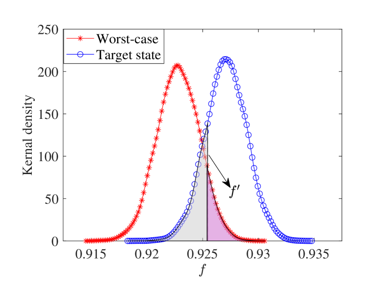
Figure 1: Illustration of the noisy QSV with two types of errors. We consider the verification of a five-qubit stabilizer state under a noise model given in Sec. IV, where ${\lambda_{0}\sim 0.9271}$ and ${\nu(\tilde{\Omega})\sim 0.4341}$. The infidelity is chosen as ${\epsilon=0.01}$. The horizontal axis $f$ is the frequency of the number of passed measurements among ${N=20000}$ measurements. The vertical axis is the kernel density function computed from $10000$ experiments. We plot the kernel density distribution for both the target state and the worst-case state. The type I and II errors correspond to the areas shaded in gray and pink respectively, which are dependent on the threshold frequency $f^{\prime}$ that we set, shown as the black vertical line.

Hence, type I and II errors are given by $F^{\leftarrow}\bigl{(}f^{\prime}N;N,\lambda_{0}\bigr{)}$ and $F^{\rightarrow}\bigl{(}f^{\prime}N;N,\lambda_{0}-\nu(\tilde{\Omega})\epsilon\bigr{)}$ respectively. If we take symmetric testing, that is to consider both type I and II errors simultaneously, the average error rate is

$$\mathrm{P}_{\text{ave}}=qF^{\leftarrow}\bigl{(}f^{\prime}N;N,\lambda_{0}\bigr{)}+(1-q)F^{\rightarrow}\bigl{(}f^{\prime}N;N,\lambda_{0}-\nu(\tilde{\Omega})\epsilon\bigr{)}\,,$$ (7)

with ${q\in\left[0,1\right]}$. Assume that the probability for either of the two types of errors to occur is the same, the average error rate is

$$\mathrm{P}_{\text{sym}}=\frac{F^{\leftarrow}\bigl{(}f^{\prime}N;N,\lambda_{0}\bigr{)}+F^{\rightarrow}\bigl{(}f^{\prime}N;N,\lambda_{0}-\nu(\tilde{\Omega})\epsilon\bigr{)}}{2}\,.$$ (8)

According to Fig. 1, the optimal choice of $f^{\prime}$ should be the intersection point of the two binomial distributions, as $\mathrm{P}_{\text{sym}}$ is the sum of two shaded areas and its minimal value is obtained when $f^{\prime}$ is the intersection of the two binomial distributions. For simplicity, we choose

$$f^{\prime}=\frac{\lambda_{0}+\lambda_{0}-\nu(\tilde{\Omega})\epsilon}{2}$$ (9)

as the threshold frequency to compute the error rate $\mathrm{P}_{\text{sym}}$. This is reasonable as the two kernel distribution curves have similar shapes when $\nu(\tilde{\Omega})\epsilon$ is small enough as compared to $\lambda_{0}$.

In order to achieve the confidence level $1-\delta$, it is required that

$$\mathrm{P}_{\text{sym}}\leq\delta\,,$$ (10)

which concludes the sample complexity of the noisy QSV protocol. A numerical simulation is illustrated in Fig. 2, which indicates that the sample complexity $N$ exhibits a nearly negative quadratic relationship with the infidelity $\epsilon$, i.e., ${N\sim\epsilon^{-2}}$ under noisy QSV. This relationship becomes more evident when considering the Chernoff bound as a binomial tail bound; see the details in Appendix C. The theoretical results we have obtained differ from certain experimental findings [45, 46, 47], where the sample complexity $N$ is approximately ${N\sim\epsilon^{-1}}$. In these experiments, the error rate, denoted by $\mathrm{P}$, is described by

$$\mathrm{P}=e^{-N\mathcal{D}(f\mid\mid 1-\nu(\Omega)\epsilon)}\leq\delta\,.$$ (11)

Note that Eq. (11) adopts asymmetric hypothesis testing, i.e., only Type I or Type II error is considered, whereas our approach involves symmetric hypothesis testing to determine the sample complexity.

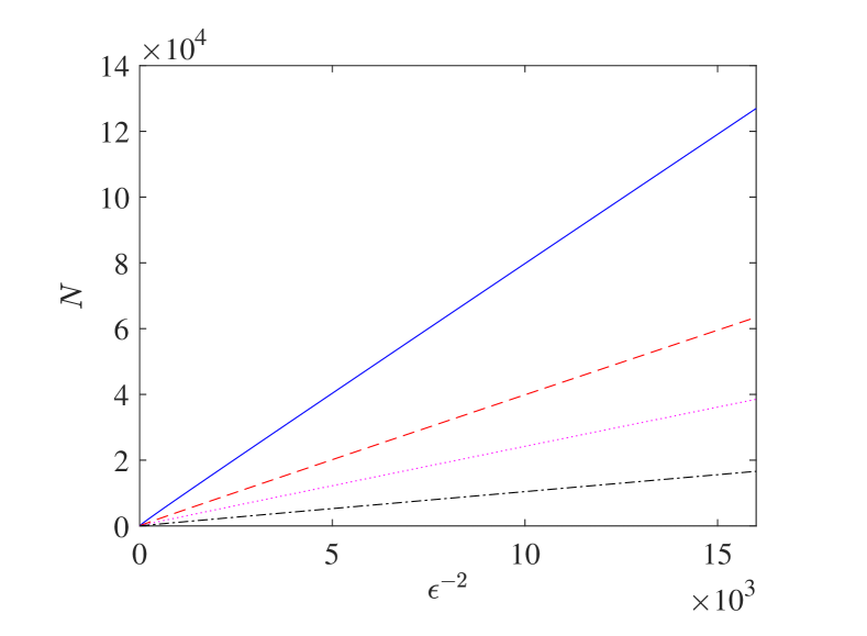
Figure 2: Noisy verification of a five-qubit stabilizer state. The simulated noisy strategy has the dominant eigenvalue ${\lambda_{0}\sim 0.9271}$ and the second-largest eigenvalue ${\lambda_{1}\sim 0.4930}$. Four curves are plotted for different confidence levels $\delta=0.01,0.05,0.1,0.2$ (top to bottom).

The results indicate that if we relax the completeness condition, i.e., the verification protocol is not necessarily required to accept the target state, the sample complexity immediately exhibits a linear relationship with $\epsilon^{-2}$, reaching the standard quantum limit. Based on the discussion, we can enhance the QSV protocol for greater precision and effectiveness in experiments, as outlined in Algorithm 1.

1

Input: The unknown state $\rho$, the infidelity $\epsilon$, the confidence level $1-\delta$, and a noisy strategy $\tilde{\Omega}=\sum_{i}p_{i}\tilde{\Omega}_{i}$ satisfying the distinguishable conditions.

Output: Determine whether $\mathcal{H}_{0}$ or $\mathcal{H}_{1}$ is true with confidence level $1-\delta$.

2 Calculate the dominant eigenvalue $\lambda_{0}$ and the spectral gap $\nu(\tilde{\Omega})$ of $\tilde{\Omega}$. 

3Get the number of measurements $N$ according to Eq. (10). 

4Randomly employ a test $\tilde{\Omega}_{i}$ from $\tilde{\Omega}$ with probability $p_{i}$ for $N$ runs. 

5Calculate the pass frequency $f$. 

6If $f\geq f^{\prime}$, accept that the unknown state $\rho$ is in $\mathcal{H}_{0}$; otherwise, accept that the unknown state is in $\mathcal{H}_{1}$.

Algorithm 1 Noisy QSV

IV Noisy verification of stabilizer states

To substantiate the validity of the theoretical framework, in this section we conduct verification experiments on five-qubit stabilizer states and GHZ states. For analytical convenience, the noise amplitudes are intentionally set along the $X$, $Y$, and $Z$ directions of the local Pauli measurements to be the same. These experiments aim to illustrate the correlation between the noise amplitude and confidence level under given conditions, notably with infidelity ${\epsilon=0.01}$ and number of measurements ${N=20000}$.

An $n$-qubit stabilizer state $|\psi\rangle$ with its stabilizer group $G=\{G_{k}\}$ can be verified by the following strategy [29]

$$\Omega_{\mathrm{S}} =\frac{1}{2^{n}-1}\sum_{G_{k}\in G\setminus\{\mathbbm{1}\}}E_{k}\,,$$ (12)

where $E_{k}=\frac{1}{2}\bigl{(}G_{k}+\mathbbm{1}\bigl{)}$ corresponds to the projection onto the positive eigensubspace of the group element $G_{k}$. The readout noise $\Lambda$ can be expressed as [49]:

$$\begin{pmatrix}\tilde{\Pi}_{1}\\ \tilde{\Pi}_{2}\\ \vdots\par\end{pmatrix}=\Lambda\begin{pmatrix}\Pi_{1}\\ \Pi_{2}\\ \vdots\end{pmatrix}\,,$$ (13)

where $\Pi_{i}$s are ideal measurements satisfying ${\sum_{i}\Pi_{i}=\mathbbm{1}}$. During the experiment, the ideal measurement $\Pi_{i}$ is replaced by the noisy measurement $\tilde{\Pi}_{i}$. Note that the noisy POVM $\bigl{\{}\tilde{\Pi}_{i}\bigr{\}}$ is still valid, implying that $\Lambda$ is a left-stochastic matrix satisfying $\sum_{j}\Lambda_{i,j}=1$. For two-outcome ideal measurements, the noisy POVM elements are

$$\tilde{\Pi}_{1} =(1-\eta)\Pi_{1}+q\Pi_{2}\,,$$ (14)

$$\tilde{\Pi}_{2} =\eta\Pi_{1}+(1-q)\Pi_{2}\,,$$

As an example of the noisy model satisfying the distinguishable conditions, we consider the case when ${\eta=q}$, that is

$$\begin{pmatrix}\tilde{\Pi}_{1}\\ \tilde{\Pi}_{2}\end{pmatrix}=\begin{pmatrix}1-\eta&\eta\\ \eta&1-\eta\end{pmatrix}\begin{pmatrix}\Pi_{1}\\ \Pi_{2}\end{pmatrix}.$$ (15)

It follows that under this condition, readout noise will only affect the eigenvalues with a noise factor, which we denote by $g$. Taking Pauli-$X$ measurement as an example with

$$\Pi_{X+} =\frac{\mathbbm{1}+X}{2}\,,\quad\Pi_{X-}=\frac{\mathbbm{1}-X}{2}\,,$$ (16)

the noisy measurements are

$$\tilde{\Pi}_{X+} =\frac{1}{2}\bigl{[}\mathbbm{1}+(1-2\eta)X\bigr{]}\,,$$ (17)

$$\tilde{\Pi}_{X-} =\frac{1}{2}\bigl{[}\mathbbm{1}-(1-2\eta)X\bigr{]}\,.$$

Compared with the ideal measurement, $\Big{\{}\tilde{\Pi}_{X+},\tilde{\Pi}_{X-}\Big{\}}$ only differs by a noise factor $g=1-2\eta$.

For $n$-qubit Pauli measurements $\bigg{\{}\frac{\mathbbm{1}+\otimes_{i}^{n}P_{i}}{2},\frac{\mathbbm{1}-\otimes_{i}^{n}P_{i}}{2}\bigg{\}}$ with $P_{i}\in\{X,Y,Z\}$ acting on the $i$-th qubit, we have

$$\frac{\mathbbm{1}+\bigotimes_{i}^{n}P_{i}}{2}$$ (18)

$$= \frac{1}{2}\bigg{(}\bigotimes_{i}^{n}\Big{(}\Pi_{i}(+)+\Pi_{i}(-)\Big{)}+\bigotimes_{i}^{n}\Big{(}\Pi_{i}(+)-\Pi_{i}(-)\Big{)}\bigg{)}$$

where $\Pi_{i}(+)$ and $\Pi_{i}(-)$ are positive and negative projective measurements on the $i$-th qubit respectively. If the readout errors affecting each qubit are uncorrelated, we have the noise model [49]

$$\Lambda=\bigotimes_{i}\Lambda_{i}\,,$$ (19)

where $\Lambda_{i}$ is the readout noise affecting the two-outcome measurement on the $i$-th qubit. Moreover, if each $\Lambda_{i}$ is analogous to Eq. (15), the noisy version of measurement $\frac{\mathbbm{1}+\otimes_{i}^{n}P_{i}}{2}$ reads

$$\frac{\bigotimes_{i}^{n}\Big{(}\tilde{\Pi}_{i}(+)+\tilde{\Pi}_{i}(-)\Big{)}+\bigotimes_{i}^{n}\Big{(}\tilde{\Pi}_{i}(+)-\tilde{\Pi}_{i}(-)\Big{)}}{2}$$ (20)

$$= \frac{\mathbbm{1}+\prod_{i}^{n}(1-2\eta_{i})\bigotimes_{i}^{n}P_{i}}{2}$$

with $\Lambda_{i}=\begin{pmatrix}1-\eta_{i}&\eta_{i}\\ \eta_{i}&1-\eta_{i}\end{pmatrix}$, which still acts as a noise factor $g=\prod_{i}^{n}(1-2\eta_{i})$ before the Pauli operator $\bigotimes_{i}^{n}P_{i}$.

Under the assumptions in Eqs. (15) and (19), measurement noise only introduces a noise factor $g$ which depends on the multi-qubit Pauli measurement. Then Proposition 1 in the following is evident. Note that Eqs. (15) and (19) serve as sufficient conditions only for the distinguishable conditions. In Sec. V we discuss the scenario where the distinguishable conditions are not met by considering $W$ state as an example.

Proposition 1.

The verification strategy $\Omega_{\mathrm{S}}$ of the stabilizer states $|\psi\rangle$ could maintain the distinguishable conditions if the readout noise satisfies the conditions in Eqs. (15) and (19). The dominant eigenvalue is $\frac{1}{2^{n}-1}\sum_{k}\frac{1}{2}(g_{k}+1)$, where $g_{k}$ denotes the noise parameter of the Pauli measurement.

The proof can be found in Appendix D. Proposition 1 guarantees that the verification strategy in Eq. (12) retains its ability to verify the target state even in the presence of measurement noise and also provides the spectral gap $\nu(\tilde{\Omega})$ used in Algorithm 1. With Proposition 1, we consider the noisy verification of a five-qubit stabilizer state with its stabilizer group $\{G_{k}\}$ generated by $\langle XZZX\mathbbm{1},\mathbbm{1}XZZX,X\mathbbm{1}XZZ,ZX\mathbbm{1}XZ,ZZZZZ\rangle$. The simulation results are shown in Fig. 3. The theoretical values are provided by Eq. (10), while simulation results are obtained by Algorithm 2 below. Figure 3 shows that the confidence level depends negatively with the noise amplitude, which supports Eq.(10).

1

Input: The unknown machine randomly generates target state $|\psi\rangle$ or worst-case state $\rho$ with the infidelity $\epsilon$ and a noisy strategy $\tilde{\Omega}=\sum_{i}p_{i}\tilde{\Omega}_{i}$ depending on a noisy parameter $g$.

Output: Determine whether $\mathcal{H}_{0}$ or $\mathcal{H}_{1}$ is true with confidence level $1-\delta$.

2 Generate state $\rho$ as either the target state $|\psi\rangle$ or a worst-case noisy state with equal probabilities. 

3Randomly employ a test $\tilde{\Omega}_{i}$ from $\tilde{\Omega}$ with probability $p_{i}$ for $N=20000$ runs. 

4We accept or reject the quantum state $\rho$ generated in step 1 with the verification protocol in Algorithm 1. If neither type I nor type II error occurs in the verification result, we call it correct. 

5Repeat Step 1 to Step 3 10000 times, simulated confidence level is the percentage of the correct results. 

6Calculate the theoretical confidence level according to Eq. (10).

Algorithm 2 Simulated experiment on noisy QSV

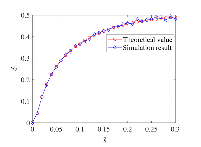
Figure 3: Simulation and theoretical results on a five-qubit stabilizer state noisy verification. The vertical axis labels the confidence level $\delta$ and the horizontal axis $g$ denotes the noisy amplitude. For convenience, the noise amplitude is chosen to be the same in all directions. The simulation settings are of sample complexity $N=20000$, infidelity $\epsilon=0.01$ with 10000 times repetition.

In another example we consider $n$-qubit GHZ states,

$$\text{{\hbox{ | \text{GHZ}_n \rangle}}}=\frac{1}{\sqrt{2}}\Bigl{(}\text{{\hbox{ | 0 \rangle}}}^{\otimes n}+\text{{\hbox{ | 1 \rangle}}}^{\otimes n}\Bigr{)}\,.$$ (21)

The verification strategy $\Omega_{\mathrm{I}}$ reads [35]

$$\Omega_{\mathrm{I}}:=\frac{1}{3}\left(P_{0}+\frac{1}{2^{n-2}}\sum_{\mathcal{Y}}P_{\mathcal{Y}}\right)=\frac{1}{3}\Bigl{(}\mathbbm{1}+2\text{{\hbox{ | \text{GHZ}_{n} \rangle}}}\text{{\hbox{ \langle\text{GHZ}_{n} | }}}\Bigr{)}\,,$$ (22)

where

$$P_{0} =\bigl{(}\text{$|0\rangle$}\text{$\langle 0|$}\bigr{)}^{\otimes{n}}+\bigl{(}\text{$|1\rangle$}\text{$\langle 1|$}\bigr{)}^{\otimes{n}}\,,$$ (23)

$$P_{\mathcal{Y}} =\frac{1}{2}\left(\mathbbm{1}+(-1)^{t}\prod_{k\in\mathcal{Y}}Y_{k}\prod_{k^{\prime}\in\bar{\mathcal{Y}}}X_{k^{\prime}}\right).$$

The spectral gap is ${\nu\bigl{(}\Omega_{\mathrm{I}}\bigr{)}=2/3}$. Based on the aforementioned discussion of the readout noise, the noisy strategy $\tilde{\Omega}_{\mathrm{I}}$ can be expressed as

$$\tilde{\Omega}_{\mathrm{I}}=\frac{1}{3}\left(\tilde{P}_{0}+\frac{1}{2^{n-2}}\sum_{\mathcal{Y}}\tilde{P}_{\mathcal{Y}}\right)$$ (24)

$$=\frac{1}{3}\left[\tilde{P}_{0}+\frac{1}{2^{n-2}}\sum_{\mathcal{Y}}\frac{1}{2}\left(\mathbbm{1}+(-1)^{t}g_{\mathcal{Y}}\prod_{k\in\mathcal{Y}}Y_{k}\prod_{k^{\prime}\in\bar{\mathcal{Y}}}X_{k^{\prime}}\right)\right],$$

where $\tilde{P}_{0}$ and $\tilde{P}_{\mathcal{Y}}$ are the noisy versions of the tests ${P}_{0}$ and ${P}_{\mathcal{Y}}$, respectively. The expression of $\tilde{P}_{0}$ is displayed in Eq. (52) in Appendix E. Similarly, if the readout noise can maintain certain special conditions as in Eqs. (15) and (19), the noisy strategy $\tilde{\Omega}_{\mathrm{I}}$ could satisfy the distinguishable conditions, as outlined in the following proposition.

Proposition 2.

The verification strategy $\Omega_{\mathrm{I}}$ for GHZ state satisfies the distinguishable conditions for readout noise stated in Eqs. (15),  (19), and  (54).

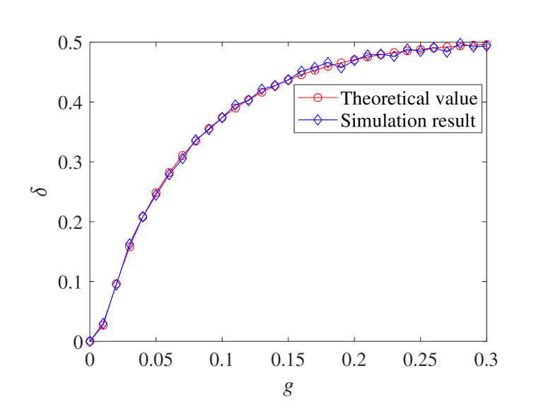
Figure 4: Simulation and theoretical results on a five-qubit GHZ state noisy verification. The vertical axis labels the confidence level $\delta$ and the horizontal axis $g$ denotes the noisy amplitude. For convenience, the noise amplitude is chosen to be the same in all directions. The simulation experiment settings are of sample complexity $N=20000$, infidelity $\epsilon=0.01$ with 10000 times repetition.

The proof can be found in Appendix E. Similar to Proposition 1, Proposition 2 demonstrates that with noisy measurements, strategy $\Omega_{\mathrm{I}}$ is still able to uniquely distinguish GHZ states. Similar to what is shown in Fig. 3, Fig. 4 demonstrates that with ${N=20000}$ measurements, high precision verification can be achieved when the noise amplitude $g_{k}$ is relatively low. As the noise amplitude $g_{k}$ increases, we can maintain a given confidence level by increasing the number of measurements. This also illustrates the correctness of the theoretical framework.

As can be seen, even if the sample complexity degrades to the standard quantum scaling, it still grows polynomially with the number of measurements $N$, implying that our protocol still enables efficient verification of entangled states through noisy measurements. Note that Propositions 1 and 2 rely on the distinguishable conditions. For those scenarios without the distinguishable conditions, we will demonstrate in the next section that a noisy strategy may still be capable of distinguishing the target state $|\psi\rangle$ from bad states in $\mathcal{H}_{1}$, which can be ascertained by semidefinite programming.

V Discussions

In the preceding section, we have discussed the noisy verification strategy that satisfies the distinguishable conditions, whereas for general target state verification and noise models such as the coherent noise, these conditions may not be fulfilled. Nevertheless, it is still possible to distinguish the null hypothesis $\mathcal{H}_{0}$ from the alternative hypothesis $\mathcal{H}_{1}$ as illustrated below.

For an $n$-qubit $W$ state

$$\text{{\hbox{ | W_n \rangle}}}=\frac{1}{\sqrt{n}}\Bigl{(}\text{{\hbox{ | 0\cdots 01 \rangle}}}+\text{{\hbox{ | 0\cdots 10 \rangle}}}+\cdots+\text{{\hbox{ | 1\cdots 00 \rangle}}}\Bigr{)}\,,$$ (25)

there exists a nonadaptive verification strategy [31]

$$\Omega_{W}=\frac{1}{2}\mathcal{Z}^{1}+\frac{1}{2C_{n}^{2}}\sum_{i<j}\Omega_{i,j}\,,$$ (26)

with $\mathcal{Z}^{1}=\sum_{u\in B_{n,1}}\text{$|u\rangle$}\text{$\langle u|$}$, $\Omega_{i,j}=\overline{\mathcal{Z}}_{i,j}^{0}(XX)_{i,j}^{+}+\overline{\mathcal{Z}}_{i,j}^{1}(\mathbbm{1}\mathbbm{1})_{i,j}$. $B_{n,1}$ denotes the set of strings in $\{0,1\}^{n}$ with Hamming weight 1, and $\overline{\mathcal{Z}}_{i,j}^{k}$ means that $k$ excitations are observed in Pauli-$Z$ measurement except for $i$ and $j$. Under the measurement noise as described in Eq.(19), the noisy strategy $\tilde{\Omega}_{W}$ is given by

$$\tilde{\Omega}_{W}=\frac{1}{2}\tilde{\mathcal{Z}}^{1}+\frac{1}{2C_{n}^{2}}\sum_{i<j}\tilde{\Omega}_{i,j}\,,$$ (27)

where $\tilde{\mathcal{Z}}^{1}=\sum_{u\in B_{n,1}}\tilde{\Pi}_{u}$, with $\tilde{\Pi}_{u}$ being the noisy version of the projector $|u\rangle$$\langle u|$. $\tilde{\Omega}_{i,j}$ is similar to $\tilde{\mathcal{Z}}^{1}$, except for the measurements that are on the $i$-th and $j$-th qubits.

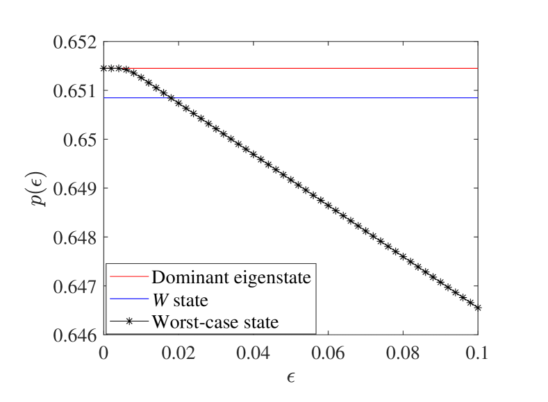
Figure 5: Simulation results on a three-qubit $W$ state noisy verification. The vertical axis labels the probability $p(\epsilon)$ of passing noisy nonadaptive strategy $\tilde{\Omega}_{W}$ and the horizontal axis denotes the infidelity $\epsilon$. The red line is the dominant eigenvalue of noisy strategy $\tilde{\Omega}_{W}$. The blue line represents the passing probability of the noisy strategy $\tilde{\Omega}_{W}$ for the $W$ state. The black line indicates the passing probability calculated for the worst-case scenario using the SDP in Eq. (28). For convenience, the noise amplitude ${g\sim 0.24}$ is chosen to be the same in all directions.

Generally $|W_{n}\rangle$ is not an eigenstate of the noisy strategy $\tilde{\Omega}_{W}$. Its passing probability ${\lambda^{\prime}=\mathrm{Tr}\Bigl{(}\tilde{\Omega}_{W}\text{$|W_{n}\rangle$}\text{$\langle W_{n}|$}\Bigr{)}}$ is smaller than the dominant eigenvalue $\lambda_{0}$ of the noisy strategy $\tilde{\Omega}_{W}$, which indicates that the distinguishable conditions are not met. For an arbitrary noisy strategy $\tilde{\Omega}$, the worst-case pass probability can be obtained by using semidefinite programming,

$$p(\epsilon)=\max_{\begin{subarray}{c}\text{$\langle\psi|$}\rho\text{$|\psi\rangle$}\leq 1-\epsilon\\ \rho\succeq 0\\ \mathrm{Tr}(\rho)=1\end{subarray}}\mathrm{Tr}(\rho\tilde{\Omega})\,,$$ (28)

and the infidelity threshold $\epsilon_{\text{th}}$ is given by $\max_{\epsilon}p(\epsilon)=\lambda^{\prime}$. Because of the monotonicity of $p(\epsilon)$, the existence of an infidelity threshold $\epsilon_{\text{th}}$ requires $p(1)<\lambda^{\prime}$, which means the pass probability of any state orthogonal to the target state $|\psi\rangle$ is less than $\lambda^{\prime}$. Since all states orthogonal to the target state are $\mathbbm{1}-\text{$|\psi\rangle$}\text{$\langle\psi|$}$ and includes $2^{n}-1$ states, we have $\mathrm{Tr}\bigl{[}(\mathbbm{1}-\text{$|\psi\rangle$}\text{$\langle\psi|$})\tilde{\Omega}\bigr{]}<(2^{n}-1)\lambda^{\prime}$. This implies that

$$\mathrm{Tr}\bigl{(}\tilde{\Omega}\bigr{)}<2^{n}\lambda^{\prime}$$ (29)

holds true. Note that Eq. (29) is a necessary condition for the existence of infidelity threshold $\epsilon_{\text{th}}$. If Eq. (29) is violated, $\epsilon_{\text{th}}$ does not exist. However, even if Eq. (29) holds, we still need to employ SDP to obtain the threshold $\epsilon_{\text{th}}$. When ${\epsilon>\epsilon_{\text{th}}}$, there is ${p(\epsilon)<\lambda^{\prime}}$, and the target state $|\psi\rangle$ is verifiable through Algorithm 1 with ${f^{\prime}=\frac{p(\epsilon)+\lambda^{\prime}}{2}}$. The numerical results are depicted in Fig. 5, where the infidelity threshold is ${\epsilon_{\text{th}}\approx 0.018}$. This means that when ${\epsilon>0.18}$, the noisy strategy $\tilde{\Omega}_{W}$ is still feasible to verify $|W_{n}\rangle$ from the bad case.

VI Conclusion

Efficient verification of entangled states with imperfect measurement apparatus is of practical interest for various quantum information processing tasks. In this work, we investigated the QSV protocols under noisy measurements. When the distinguishable conditions are met, the noisy QSV strategy is still faithful to verify the target state. However, due to the measurement noise, both type I and type II errors can happen in the hypothesis testing framework as described in Algorithm 1. Our results show that the sample complexity $N$ exhibits a negative quadratic relation with the infidelity $\epsilon$ for symmetric hypothesis testing. Besides, the theoretical framework is supplemented with numerical experiments on stabilizer states and GHZ states. Moreover, violation of the distinguishable conditions is discussed for the verification of $W$ states, where the noisy strategy can identify the bad states with infidelity larger than a threshold value. Our work illustrates the potential for efficient verification of various entangled states of interest using existing verification strategies, avoiding the need for more complex experimental settings. Furthermore, our protocols have the potential to support robust noisy verification in the future.

Appendix A Proof of Observation 1

Here we prove that the distinguishable conditions are necessary and sufficient for a strategy $\Omega$ to uniquely identify the target state $|\psi\rangle$ from any other state.

Proof.

Suppose the spectral decomposition of a strategy $\Omega$ is

$$\Omega=\sum_{i=0}^{d-1}{\lambda_{i}}\text{{\hbox{ | \phi_i \rangle}}}\text{{\hbox{ \langle\phi_i | }}}\,,$$ (30)

where $\lambda_{i}\geq\lambda_{j}$ for $i<j$, and $\big{\{}\text{$|\phi_{i}\rangle$}\big{\}}$ form an orthonormal basis in the Hilbert space.

Firstly, we prove the sufficiency of the distinguishable conditions, i.e., that if the strategy satisfies the distinguishable conditions, where the target state $|\psi\rangle$ is the dominant eigenstate $|\phi_{0}\rangle$ with eigenvalue $\lambda_{0}$, then it can uniquely distinguish the target state from any other state. For any pure state $|\phi^{\prime}\rangle$ other than $|\phi_{0}\rangle$, its decomposition reads

$$\text{{\hbox{ | \phi^{\prime} \rangle}}}=a\text{{\hbox{ | \phi_0 \rangle}}}+b\text{{\hbox{ | \phi_0^{\bot} \rangle}}}$$ (31)

where $|\phi_{0}^{\bot}\rangle$ is orthogonal to $|\phi_{0}\rangle$, $\left|a\right|^{2}+\left|b\right|^{2}=1$, $|b|>0$. Direct calculation shows

$$\mathrm{Tr}\bigl{(}\Omega\text{$|\phi^{\prime}\rangle$}\text{$\langle\phi^{\prime}|$}\bigr{)} =\text{$\langle\phi^{\prime}|$}\Omega\text{$|\phi^{\prime}\rangle$}$$ (32)

$$=a^{*}a\text{$\langle\phi_{0}|$}\Omega\text{$|\phi_{0}\rangle$}+a^{*}b\text{$\langle\phi_{0}|$}\Omega\text{$|\phi_{0}^{\bot}\rangle$}+b^{*}a\text{$\langle\phi_{0}^{\bot}|$}\Omega\text{$|\phi_{0}\rangle$}+b^{*}b\text{$\langle\phi_{0}^{\bot}|$}\Omega\text{$|\phi_{0}^{\bot}\rangle$}$$

$$=\left|a\right|^{2}\lambda_{0}+\left|b\right|^{2}\text{$\langle\phi_{0}^{\bot}|$}\Omega\text{$|\phi_{0}^{\bot}\rangle$}<\lambda_{0}\,.$$

So for any pure state $|\phi^{\prime}\rangle$ other than $|\phi_{0}\rangle$, the probability $\mathrm{Tr}(\Omega\text{$|\phi^{\prime}\rangle$}\text{$\langle\phi^{\prime}|$})$ must be less than $\lambda_{0}$. Moreover, for any mixed state $\rho=\sum_{i}p_{i}\text{$|\psi_{i}\rangle$}\text{$\langle\psi_{i}|$}$,

$$\mathrm{Tr}(\rho\Omega)=\sum_{i}p_{i}\bigl{(}\Omega\text{{\hbox{ | \psi_i \rangle}}}\text{{\hbox{ \langle\psi_i | }}}\bigr{)}<\sum_{i}p_{i}\bigl{(}\Omega\text{{\hbox{ | \phi_0 \rangle}}}\text{{\hbox{ \langle\phi_0 | }}}\bigr{)}=\lambda_{0}\,.$$ (33)

Thus, strategy $\Omega$ can distinguish any other state from the target state $|\psi\rangle$.

Next, we show that the distinguishable conditions are necessary for a noisy strategy $\Omega$ to uniquely identify the target state $|\psi\rangle$. If the dominant eigenstate $|\phi_{0}\rangle$ is not the target state $|\psi\rangle$, then

$$\text{{\hbox{ | \psi \rangle}}}=\sqrt{1-\varepsilon}\text{{\hbox{ | \phi_0 \rangle}}}+\sqrt{\varepsilon}\text{{\hbox{ | \phi_0^{\bot} \rangle}}}\,,$$ (34)

where $0<\varepsilon\leq 1$. There exists another state

$$\text{{\hbox{ | \psi' \rangle}}}=\sqrt{1-\varepsilon}\text{{\hbox{ | \phi_0 \rangle}}}-\sqrt{\varepsilon}\text{{\hbox{ | \phi_0^{\bot} \rangle}}}\,,$$ (35)

such that

$$\mathrm{Tr}\bigl{(}\Omega\text{{\hbox{ | \psi' \rangle}}}\text{{\hbox{ \langle\psi' | }}}\bigr{)}=\mathrm{Tr}\bigl{(}\Omega\text{{\hbox{ | \psi \rangle}}}\text{{\hbox{ \langle\psi | }}}\bigr{)}\,.$$ (36)

If the spectral gap equals to 0 and the target state $|\psi\rangle$ is an eigenstate of $\Omega$ with the largest eigenvalue $\lambda_{0}$, any $|\psi^{\prime}\rangle$ in the degenerate eigensubspace for $\lambda_{0}$ satisfies Eq. (36). Thus, a noisy verification strategy $\tilde{\Omega}$ can uniquely distinguish the target state iff it meets the distinguishable conditions. ∎

Appendix B Proof of Eqs. (3) and  (4)

Here we prove that if the distinguishable conditions are met, the worst-case state is in the form of a pure state as in Eq. (3).

Proof.

Under the distinguishable conditions, the spectral decomposition of a noisy strategy $\tilde{\Omega}$ could be written as

$$\tilde{\Omega}=\lambda_{0}\text{{\hbox{ | \psi \rangle}}}\text{{\hbox{ \langle \psi | }}}+\sum_{i=1}\lambda_{i}\text{{\hbox{ | \psi^{\perp}_{i} \rangle}}}\text{{\hbox{ \langle \psi^{\perp}_{i} | }}}\,,$$ (37)

where $|\psi\rangle$ is the target state with dominant eigenvalue $\lambda_{0}$, and the worst-case state $\sigma$ reads

$$\sigma=r\text{{\hbox{ | \psi \rangle}}}\text{{\hbox{ \langle \psi | }}}+(1-r)\sigma^{\perp}+c\text{{\hbox{ | \psi \rangle}}}\text{{\hbox{ \langle\Phi^{\perp} | }}}+c^{*}\text{{\hbox{ | \Phi^{\perp} \rangle}}}\text{{\hbox{ \langle \psi | }}}\,.$$ (38)

The worst-case $\sigma$ maximizes $\mathrm{Tr}(\tilde{\Omega}\sigma)$ as follows

$$\max_{\sigma}\mathrm{Tr}(\tilde{\Omega}\sigma)=\max_{\sigma}\Bigg{[}\lambda_{0}\text{{\hbox{ \langle \psi | }}}\sigma\text{{\hbox{ | \psi \rangle}}}+\mathrm{Tr}\biggl{(}\sum_{i}\lambda_{i}\text{{\hbox{ | \psi^{\perp}_{i} \rangle}}}\text{{\hbox{ \langle \psi^{\perp}_{i} | }}}\sigma\biggr{)}\Bigg{]}=r\lambda_{0}+(1-r)\lambda_{1}=\lambda_{1}+r\bigr{(}\lambda_{0}-\lambda_{1}\bigl{)}\,,$$ (39)

where the optimal $\sigma^{\perp}=\text{$|\psi^{\perp}_{1}\rangle$}\text{$\langle\psi^{\perp}_{1}|$}$ is the eigenstate corresponding to the second-largest eigenvalue $\lambda_{1}$ of $\tilde{\Omega}$. Note $\text{$\langle\psi|$}\sigma\text{$|\psi\rangle$}\leq 1-\epsilon$, implying $r\leq 1-\epsilon$. Therefore, $\mathrm{Tr}(\tilde{\Omega}\sigma)=\lambda_{1}+(1-\epsilon)(\lambda_{0}-\lambda_{1})=\lambda_{0}-\epsilon(\lambda_{0}-\lambda_{1})$ is maximized by choosing $r=1-\epsilon$. Hence, the worst-case scenario is achieved by a pure state $\sigma=\text{$|\psi^{\prime}\rangle$}\text{$\langle\psi^{\prime}|$}$, where $\text{$|\psi^{\prime}\rangle$}=\sqrt{1-\epsilon}\text{$|\psi\rangle$}+\sqrt{\epsilon}\text{$|\psi^{\perp}_{1}\rangle$}$. ∎

Appendix C Discussion of Chernoff bound

To establish an explicit relation between the sample complexity and noise, we employ the Chernoff bound to characterize the binomial cumulative distribution, i.e.,

$$F^{\leftarrow}(k;N,p)=\operatorname{Pr}(X\leq k)\leq e^{-\mathcal{D}\bigl{(}\,\frac{k}{N}\mid\mid p\,\bigr{)}N}\,,$$ (40)

where

$$\mathcal{D}(f\mid\mid p):=f\ln\frac{f}{p}+(1-f)\ln\frac{1-f}{1-p}$$ (41)

is the Kullback–Leibler divergence. Thus, the average error rate $\mathrm{P}_{\text{sym}}$ in Eq. (8) can be bounded as

$$\mathrm{P}_{\text{sym}} \leq\frac{e^{-\mathcal{D}\bigl{(}\,\lambda_{0}\mid\mid\lambda_{0}-\frac{1}{2}\nu(\tilde{\Omega})\epsilon\,\bigr{)}N}+e^{-\mathcal{D}\bigl{(}\,\lambda_{0}-\nu(\tilde{\Omega})\epsilon\mid\mid\lambda_{0}-\frac{1}{2}\nu(\tilde{\Omega})\epsilon\,\bigr{)}N}}{2}$$ (42)

$$=\frac{1}{2}\left[\biggl{(}\frac{\lambda_{0}-\frac{1}{2}\nu(\tilde{\Omega})\epsilon}{\lambda_{0}}\biggr{)}^{\lambda_{0}}\biggl{(}\frac{1-\lambda_{0}+\frac{1}{2}\nu(\tilde{\Omega})\epsilon}{1-\lambda_{0}}\biggr{)}^{1-\lambda_{0}}\right]^{N}+\frac{1}{2}\left[\biggl{(}\frac{\lambda_{0}-\frac{1}{2}\nu(\tilde{\Omega})\epsilon}{\lambda_{0}-\nu(\tilde{\Omega})\epsilon}\biggr{)}^{\lambda_{0}-\nu(\tilde{\Omega})\epsilon}\biggl{(}\frac{1-\lambda_{0}+\frac{1}{2}\nu(\tilde{\Omega})\epsilon}{1-\lambda_{0}+\nu(\tilde{\Omega})\epsilon}\biggr{)}^{1-\lambda_{0}+\nu(\tilde{\Omega})\epsilon}\right]^{N}\,.$$

In comparison to the standard QSV efficiency $(1-\nu(\tilde{\Omega})\epsilon)^{N}$, we could examine $\sqrt[N]{\mathrm{P}_{\text{sym}}}$ firstly

$$\sqrt[N]{\mathrm{P}_{\text{sym}}} \leq\left\{\frac{1}{2}\left[\biggl{(}\frac{\lambda_{0}-\frac{1}{2}\nu(\tilde{\Omega})\epsilon}{\lambda_{0}}\biggr{)}^{\lambda_{0}}\biggl{(}\frac{1-\lambda_{0}+\frac{1}{2}\nu(\tilde{\Omega})\epsilon}{1-\lambda_{0}}\biggr{)}^{1-\lambda_{0}}\right]^{N}\right.+\left.\frac{1}{2}\left[\biggl{(}\frac{\lambda_{0}-\frac{1}{2}\nu(\tilde{\Omega})\epsilon}{\lambda_{0}-\nu(\tilde{\Omega})\epsilon}\biggr{)}^{\lambda_{0}-\nu(\tilde{\Omega})\epsilon}\biggl{(}\frac{1-\lambda_{0}+\frac{1}{2}\nu(\tilde{\Omega})\epsilon}{1-\lambda_{0}+\nu(\tilde{\Omega})\epsilon}\biggr{)}^{1-\lambda_{0}+\nu(\tilde{\Omega})\epsilon}\right]^{N}\right\}^{\frac{1}{N}}$$ (43)

$$=1+0*\nu(\tilde{\Omega})\epsilon-\frac{1}{8\bigl{(}1-\lambda_{0}\bigr{)}\lambda_{0}}*\bigl{(}\nu(\tilde{\Omega})\epsilon\bigr{)}^{2}+...+R_{n}\bigl{(}\nu(\tilde{\Omega})\epsilon\bigr{)}\,.$$

Thus,

$$\mathrm{P}_{\text{sym}}={\biggl{(}\sqrt[N]{\mathrm{P}_{\text{sym}}}\biggr{)}}^{N}\leq\bigg{[}1+0*\nu(\tilde{\Omega})\epsilon-\frac{1}{8\bigl{(}1-\lambda_{0}\bigr{)}\lambda_{0}}*(\nu(\tilde{\Omega})\epsilon)^{2}+...+R_{n}(\nu(\tilde{\Omega})\epsilon)\bigg{]}^{N}\,.$$ (44)

If we ignore high-order items and require $\bigg{[}1-\frac{1}{8\bigl{(}1-\lambda_{0}\bigr{)}\lambda_{0}}*(\nu(\tilde{\Omega})\epsilon)^{2}\bigg{]}^{N}\leq\delta$, then

$$N\geq\frac{\ln\delta}{\ln\bigg{(}1-\frac{1}{8\bigl{(}1-\lambda_{0}\bigr{)}\lambda_{0}}*(\nu(\tilde{\Omega})\epsilon)^{2}\bigg{)}}\approx 8\bigl{(}1-\lambda_{0}\bigr{)}\lambda_{0}(\nu(\tilde{\Omega})\epsilon)^{-2}\ln\delta^{-1}\,$$ (45)

shows that the sample complexity $N$ exhibits a negative quadratic relation with both the infidelity $\epsilon$ and the spectral gap $\nu(\tilde{\Omega})$ of the noisy strategy $\tilde{\Omega}$. This implies that the sample complexity of noisy QSV remains polynomial with respect to the size of the quantum system. Additionally, apart from the spectral gap $\nu(\tilde{\Omega})$ and infidelity $\epsilon$, measurement noise further influences the sample complexity by affecting the dominant eigenvalue $\lambda_{0}$.

Appendix D Proof of Proposition 1

Here we prove that when the assumptions in Eqs. (15) and (19) hold true, the strategy $\Omega_{\mathrm{S}}$ in Eq. (12) satisfies the dintinguishable conditions.

Proof.

Recall that the stabilizer state $|\psi\rangle$ is defined by its stabilizer group $\{G_{k}\}$, the generators of which are denoted by $\langle S_{j}\rangle$. The readout noise under the assumptions in Eqs. (15) and (19) only introduces a noise factor $g_{k}=\prod_{i}^{n}(1-2\eta_{i})$ on the operator $G_{k}$, as stated in Eq. (20). Then for any test operator $E_{k}=\frac{1}{2}\bigl{(}G_{k}+\mathbbm{1}\bigr{)}$, its noisy version $\tilde{E}_{k}$ reads

$$\tilde{E}_{k}=\frac{1}{2}\Bigl{(}\tilde{G}_{k}+\mathbbm{1}\Bigr{)}=\frac{1}{2}\bigl{(}G_{k}G_{k}+\mathbbm{1}\bigr{)}\,.$$ (46)

The noisy measurement operator $\tilde{E}_{k}$ has only two eigenvalues: $\frac{1}{2}\bigl{(}G_{k}+1\bigr{)}$ and $\frac{1}{2}\bigl{(}1-G_{k}\bigr{)}$, where $G_{k}$ is the noise parameter. The stabilizer state $|\psi\rangle$ is the eigenstate with the greater eigenvalue $\frac{1}{2}\bigl{(}G_{k}+1\bigr{)}$. Moreover, the stabilizer state is the unique state that has the larger eigenvalue for each test operator $\tilde{E}_{k}$, due to the fact that the dimension of the common eigenspace of the stabilizer group elements is $d_{\mathcal{H_{G}}}=1$. Thus, the dominant eigenvalue of the noisy strategy $\tilde{\Omega}_{\mathrm{S}}$ is $\frac{1}{2^{n}-1}\sum_{k}\frac{1}{2}(G_{k}+1)$. Note that $\big{\{}E_{k}\big{\}}$ is a commutative set, consequently, $\Big{\{}\tilde{E}_{k}\Big{\}}$ are also commutative and share the same common eigenspace $\bigl{\{}\text{$|G_{\mathbf{w}}\rangle$}\bigr{\}}$. $\bigl{\{}\text{$|G_{\mathbf{w}}\rangle$}\bigr{\}}$ form the stabilizer basis labeled by vectors in the binary vector space $\mathbf{w}\in\mathbbm{Z}_{2}^{n}$, as follows

$$\text{{\hbox{ | G_{\mathbf{w}} \rangle}}}\text{{\hbox{ \langle G_{\mathbf{w}} | }}}=\Pi_{G_{\mathbf{w}}}=\prod_{j=1}^{n}\frac{\mathbbm{1}+(-1)^{w_{j}}S_{j}}{2}=\sum_{\mathbf{y}\in\mathbbm{Z}_{2}^{n}}(-1)^{\mathbf{w}\cdot\mathbf{y}}S^{\mathbf{y}}\,,$$ (47)

where $S^{\mathbf{y}}=\prod_{j=1}^{n}S_{j}^{y_{j}}$ is an element in group $\big{\{}G_{k}\big{\}}$ denoted by $\mathbf{y}\in\mathbbm{Z}_{2}^{n}$. Thus, for each stabilizer basis $|G_{\mathbf{w}}\rangle$, its pass probability of the measurement $\tilde{E}_{k}=\frac{g_{k}G_{k}+\mathbbm{1}}{2}$ reads

$$\mathrm{Tr}\biggl{(}\tilde{E}_{k}\text{$|G_{\mathbf{w}}\rangle$}\text{$\langle G_{\mathbf{w}}|$}\biggr{)} =\mathrm{Tr}\biggl{(}\sum_{\mathbf{y}\in\mathbbm{Z}_{2}^{n}}(-1)^{\mathbf{w}\cdot\mathbf{y}}S^{\mathbf{y}}\tilde{E}_{k}\biggr{)}=\frac{1}{2}\mathrm{Tr}\Bigg{[}\sum_{\mathbf{y}\in\mathbbm{Z}_{2}^{n}}(-1)^{\mathbf{w}\cdot\mathbf{y}}S^{\mathbf{y}}(g_{k}G_{k}+\mathbbm{1})\Bigg{]}$$ (48)

$$=\frac{1}{2}+\frac{g_{k}}{2}\mathrm{Tr}\biggl{(}\sum_{\mathbf{y}\in\mathbbm{Z}_{2}^{n}}(-1)^{\mathbf{w}\cdot\mathbf{y}}S^{\mathbf{y}}S^{\mathbf{k}}\biggr{)}=\frac{1}{2}\biggl{(}1+g_{k}(-1)^{\mathbf{w}\cdot\mathbf{k}}\biggr{)}\,.$$

Here, $G_{k}=S^{\mathbf{k}}$ denotes an element in the group $\big{\{}G_{k}\big{\}}$, excluding the identity element $\mathbbm{1}$, where $\mathbf{k}\in\mathbbm{Z}_{2}^{n}\setminus\{\mathbf{0}\}$. Thus, the probability $p_{\mathbf{w}}$ of passing through the noisy strategy $\tilde{\Omega}_{\mathrm{S}}$ for $|G_{\mathbf{w}}\rangle$ is

$$p_{\mathbf{w}}=\mathrm{Tr}\biggl{(}\tilde{\Omega}_{\mathrm{S}}\text{{\hbox{ | G_{\mathbf{w}} \rangle}}}\text{{\hbox{ \langle G_{\mathbf{w}} | }}}\biggr{)}=\frac{1}{2^{n}-1}\sum_{\mathbf{k}}\frac{1}{2}\Bigl{(}1+g_{k}(-1)^{\mathbf{w}\cdot\mathbf{k}}\Bigr{)}\,.$$ (49)

The maximum eigenvalue $\lambda_{1}$ can be obtained

$$\lambda_{1}=\max_{\mathbf{w}\in\mathbbm{Z}_{2}^{n}\setminus\{\mathbf{0}\}}p_{\mathbf{w}}\,.$$ (50)

∎

Appendix E Proof of Proposition 2

Here we prove that when the assumptions in Eqs. (15), (19), and (54) are met, the strategy $\Omega_{\mathrm{I}}$ in Eq. (22) could satisfy the dintinguishable conditions.

Proof.

We replace all noiseless local Pauli measurements, denoted as $\{\Pi_{X+},\Pi_{X-},\Pi_{Y+},\Pi_{Y-},\Pi_{Z+},\Pi_{Z-}\}$, with their respective noisy version represented by $\{\tilde{\Pi}_{X+},\tilde{\Pi}_{X-},\tilde{\Pi}_{Y+},\tilde{\Pi}_{Y-},\tilde{\Pi}_{Z+},\tilde{\Pi}_{Z-}\}$. For instance, noisy measurements of Pauli-$X$ could be written as

$$\left(\begin{array}[]{c}\tilde{\Pi}_{X+}\\ \tilde{\Pi}_{X-}\end{array}\right) =\Lambda_{x}\left(\begin{array}[]{l}\Pi_{X+}\\ \Pi_{X-}\end{array}\right)=\left(\begin{array}[]{cc}1-\eta_{x}&\eta_{x}\\ \eta_{x}&1-\eta_{x}\end{array}\right)\left(\begin{array}[]{l}\Pi_{X+}\\ \Pi_{X-}\end{array}\right)\,,$$ (51)

where $\eta_{x}$ is the noisy parameter of Pauli-$X$ measurement.

For test $P_{0}$ in the verification operator $\Omega_{\mathrm{I}}$, the noisy version is

$$\tilde{P}_{0}=\bigotimes_{i}\bigl{(}\tilde{\Pi}_{Z+}\bigr{)}_{i}+\bigotimes_{i}\bigl{(}\tilde{\Pi}_{Z-}\bigr{)}_{i}=\bigotimes_{i}\left[\Bigl{(}1-\eta^{i}_{z}\Bigr{)}\Pi^{i}_{Z+}+\eta^{i}_{z}\Pi^{i}_{Z-}\right]+\bigotimes_{i}\left[\eta^{i}_{z}\Pi^{i}_{Z+}+\Bigl{(}1-\eta^{i}_{z}\Bigr{)}\Pi^{i}_{Z-}\right]\,.$$ (52)

The $\eta^{i}_{z}$ is noisy parameter of measurement on $i$-th qubit and $\bigl{(}\tilde{\Pi}_{Z+}\bigr{)}_{i}$ means noisy projective measurement on $i$-th qubit.

For the first item $\bigotimes_{i}\left[\Bigl{(}1-\eta^{i}_{z}\Bigr{)}\Pi^{i}_{Z+}+\eta^{i}_{z}\Pi^{i}_{Z-}\right]$ in Eq. (52), direct calculations show

$$\bigotimes_{i}\left[\Bigl{(}1-\eta^{i}_{z}\Bigr{)}\Pi^{i}_{Z+}+\eta^{i}_{z}\Pi^{i}_{Z-}\right] =\left[\Bigl{(}1-\eta^{1}_{z}\Bigr{)}\Pi^{1}_{Z+}+\eta^{1}_{z}\Pi^{1}_{Z-}\right]\otimes\left[\Bigl{(}1-\eta^{2}_{z}\Bigr{)}\Pi^{2}_{Z+}+\eta^{2}_{z}\Pi^{2}_{Z-}\right]\otimes\cdots\otimes\left[\Bigl{(}1-\eta^{n}_{z}\Bigr{)}\Pi^{n}_{Z+}+\eta^{n}_{z}\Pi^{n}_{Z-}\right]\,.$$ (53)

It is straightforward to verify that the state $\text{$|0\rangle$}^{\otimes n}$ has an eigenvalue of $\prod_{i=1}^{n}\Bigl{(}1-\eta^{i}_{z}\Bigr{)}$, while the state $\text{$|1\rangle$}^{\otimes n}$ has an eigenvalue of $\prod_{i=1}^{n}\eta^{i}_{z}$. Similarly, for the second term in Eq. (52), the state $\text{$|1\rangle$}^{\otimes n}$ has an eigenvalue of $\prod_{i=1}^{n}\Bigl{(}1-\eta^{i}_{z}\Bigr{)}$, and the state $\text{$|0\rangle$}^{\otimes n}$ has an eigenvalue of $\prod_{i=1}^{n}\eta^{i}_{z}$. Thus, the GHZ state is an eigenspace of the noisy operator $\tilde{P}_{0}$ with eigenvalue $\prod^{n}_{i=1}\Bigl{(}1-\eta^{i}_{z}\Bigr{)}+\prod^{n}_{i=1}\eta^{i}_{z}$. We will then demonstrate the condition under which $\prod^{n}_{i}\Bigl{(}1-\eta^{i}_{z}\Bigr{)}+\prod^{n}_{i}\eta^{i}_{z}$ becomes the largest eigenvalue of the test $\tilde{P}_{0}$.

Note that the eigenvalue of $\tilde{P}_{0}$ could be expressed as $\prod\limits_{i\in A}\Bigl{(}1-\eta^{i}_{z}\Bigr{)}\prod\limits_{i\in\overline{A}}\eta^{i}_{z}+\prod\limits_{i\in\overline{A}}\Bigl{(}1-\eta^{i}_{z}\Bigr{)}\prod\limits_{i\in A}\eta^{i}_{z}$, where $A\in\{1,2,\cdots,n\}$ represents a combination of qubits from the set $\{1,2,\cdots,n\}$. When the first item $\bigotimes_{i}\left[\Bigl{(}1-\eta^{i}_{z}\Bigr{)}\Pi^{i}_{Z+}+\eta^{i}_{z}\Pi^{i}_{Z-}\right]$ in Eq. (52) takes one value of the $i$-th qubit $\Big{\{}\eta^{i}_{z},1-\eta^{i}_{z}\Big{\}}$, the second item $\bigotimes_{i}\left[\eta^{i}_{z}\Pi^{i}_{Z+}+\Bigl{(}1-\eta^{i}_{z}\Bigr{)}\Pi^{i}_{Z-}\right]$ can only take the other. If we require that $\prod^{n}_{i=1}\Bigl{(}1-\eta^{i}_{z}\Bigr{)}+\prod^{n}_{i=1}\eta^{i}_{z}$ is the largest eigenvalue among all possible combinations $\prod\limits_{i\in A}\Bigl{(}1-\eta^{i}_{z}\Bigr{)}\prod\limits_{i\in\overline{A}}\eta^{i}_{z}+\prod\limits_{i\in\overline{A}}\Bigl{(}1-\eta^{i}_{z}\Bigr{)}\prod\limits_{i\in A}\eta^{i}_{z}$, the following condition should be satisfied

$$\prod^{n}_{i=1}\Bigl{(}1-\eta^{i}_{z}\Bigr{)}+\prod^{n}_{i=1}\eta^{i}_{z}-\Bigg{[}\prod\limits_{i\in A}\Bigl{(}1-\eta^{i}_{z}\Bigr{)}\prod\limits_{i\in\overline{A}}\eta^{i}_{z}+\prod\limits_{i\in\overline{A}}\Bigl{(}1-\eta^{i}_{z}\Bigr{)}\prod\limits_{i\in A}\eta^{i}_{z}\Bigg{]}$$ (54)

$$= \Bigg{[}\prod^{n}_{i=1}\Bigl{(}1-\eta^{i}_{z}\Bigr{)}-\prod\limits_{i\in A}\Bigl{(}1-\eta^{i}_{z}\Bigr{)}\prod\limits_{i\in\overline{A}}\eta^{i}_{z}\Bigg{]}+\Bigg{[}\prod^{n}_{i=1}\eta^{i}_{z}-\prod\limits_{i\in\overline{A}}\Bigl{(}1-\eta^{i}_{z}\Bigr{)}\prod\limits_{i\in A}\eta^{i}_{z}\Bigg{]}$$

$$= \Bigg{[}\prod\limits_{i\in A}\Bigl{(}1-\eta^{i}_{z}\Bigr{)}\Biggl{(}\prod\limits_{i\in\overline{A}}\Bigl{(}1-\eta^{i}_{z}\Bigr{)}-\prod\limits_{i\in\overline{A}}\eta^{i}_{z}\Biggr{)}\Bigg{]}-\Bigg{[}\Biggl{(}\prod\limits_{i\in\overline{A}}\Bigl{(}1-\eta^{i}_{z}\Bigr{)}-\prod\limits_{i\in\overline{A}}\eta^{i}_{z}\Biggr{)}\prod\limits_{i\in A}\eta^{i}_{z}\Bigg{]}$$

$$= \Biggl{(}\prod\limits_{i\in\overline{A}}\Bigl{(}1-\eta^{i}_{z}\Bigr{)}-\prod\limits_{i\in\overline{A}}\eta^{i}_{z}\Biggr{)}\Biggl{(}\prod\limits_{i\in A}\Bigl{(}1-\eta^{i}_{z}\Bigr{)}-\prod\limits_{i\in A}\eta^{i}_{z}\Biggr{)}\geq 0\,.$$

The test $P_{\mathcal{Y}}$ in the strategy $\Omega_{\mathrm{I}}$ is similar to the test in the stabilizer state verification strategy $\Omega_{\mathrm{S}}$. Thus, Proposition 2 establishes that the GHZ state takes the dominant eigenvalue $\frac{1}{3}\left[\prod_{i=1}^{n}\Bigl{(}1-\eta^{i}_{z}\Bigr{)}+\prod_{i=1}^{n}\eta^{i}_{z}\right]+\frac{1}{3\cdot 2^{n-2}}\sum_{\mathcal{Y}}\frac{1}{2}(g_{\mathcal{Y}}+1)$ of the noisy strategy $\tilde{\Omega}_{\mathrm{I}}$, where $g_{\mathcal{Y}}$ denotes the noisy parameter dependent on the test $P_{\mathcal{Y}}$.

∎