Understanding Token Probability Encoding in Output Embeddings

Abstract

In this paper, we investigate the output token probability information in the output embedding of language models. We provide an approximate common log-linear encoding of output token probabilities within the output embedding vectors and demonstrate that it is accurate and sparse when the output space is large and output logits are concentrated. Based on such findings, we edit the encoding in output embedding to modify the output probability distribution accurately. Moreover, the sparsity we find in output probability encoding suggests that a large number of dimensions in the output embedding do not contribute to causal language modeling. Therefore, we attempt to delete the output-unrelated dimensions and find more than 30% of the dimensions can be deleted without significant movement in output distribution and degeneration on sequence generation. Additionally, in training dynamics, we use such encoding as a probe and find that the output embeddings capture token frequency information in early steps, even before an obvious convergence starts.

Understanding Token Probability Encoding in Output Embeddings

Hakaze Cho^1,∗, Yoshihiro Sakai¹, Kenshiro Tanaka¹, Mariko Kato¹, Naoya Inoue^{1,2,∗ 1}Japan Advanced Institute of Science and Technology, ²RIKEN ^∗{yfzhao, naoya-i}@jaist.ac.jp

1 Introduction

Modern Language Models (LMs) have two kinds of embeddings. One is the input embedding $E^{(i)}$ located at the earliest layer of LMs, for mapping the input token index into distributed inner representation. The other is the output embedding $E^{(o)}$ in the Language Modeling head (LM head), for mapping the hidden state to the predicted probability distribution of the next token in the causal language modeling task.

Since the output embeddings were often tied with the input embeddings Chung et al. (2020); Press and Wolf (2017), i.e. input embeddings are directly used as the output embedding, the behaviors and features of independent output embeddings are rarely investigated. Along with the scaling of LMs, such embedding tying, which is proven to be harmful to model performance Chung et al. (2020), is gradually being unused in modern LMs such as GPT-J Wang and Komatsuzaki (2021) and LLaMa 2 Touvron et al. (2023). This raises attention to the output embeddings, and explaining its underlying mechanism can be beneficial to understanding and improving LMs.

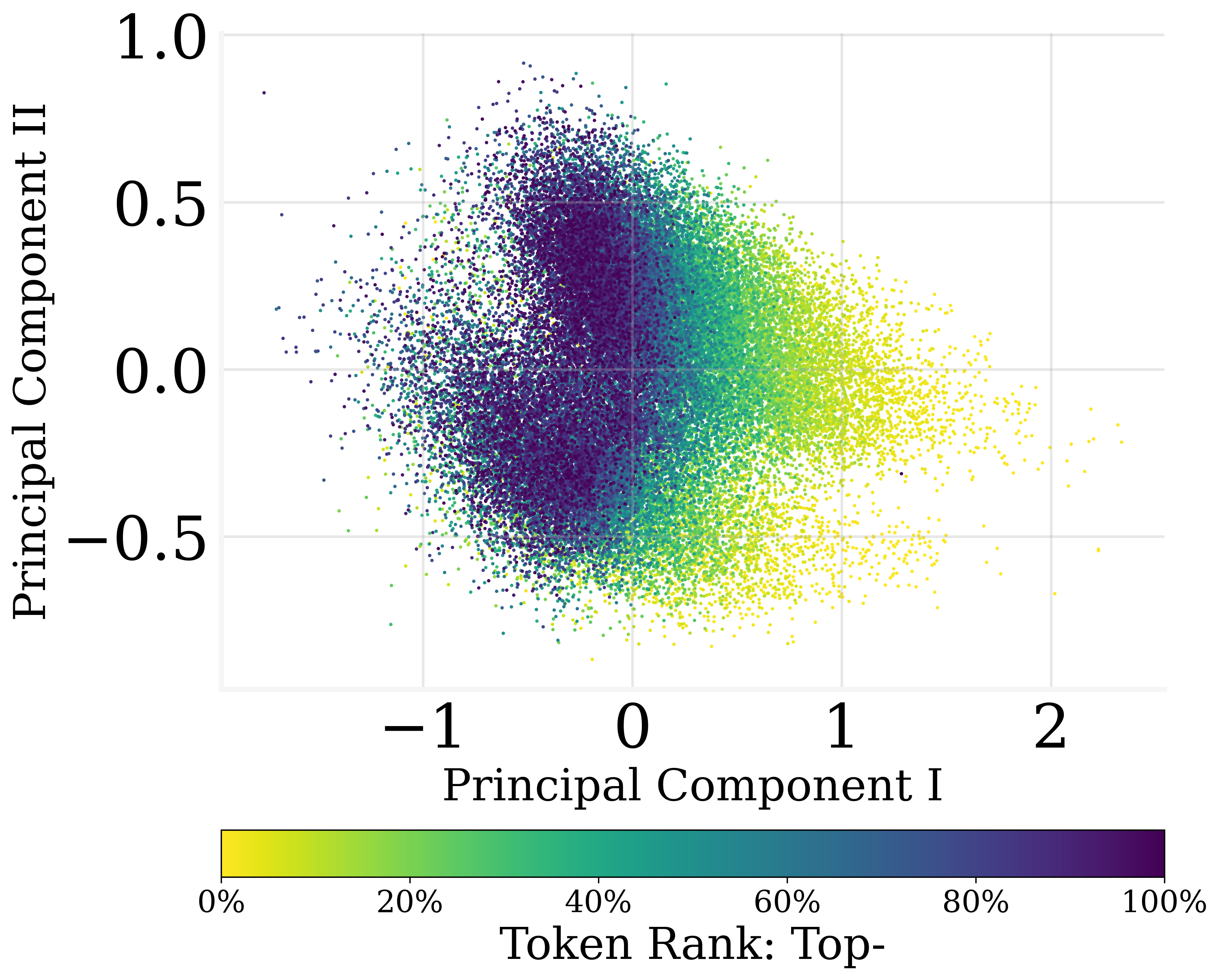
Figure 1: The PCA result of the output embedding parameters of GPT2. Colors refer to the ranking percentile of the averaged output token probability. Output embeddings encode the probabilities linear-likely.

The most obvious and expected role of the LM heads is to map the last hidden states into token probabilities. Therefore, following Kobayashi et al. (2023), who found an encoding of the averaged output token probability distribution in the bias term of the output LM head, this paper also focuses on the averaged output probabilities as an overall representation of LM outputs. We observe there is a linear-like correlation between the output token probabilities and the output embedding as shown in Fig. 1. In §2, our mathematical derivation indicates that $\mathrm{softmax}$ LM head naturally encodes the output probabilities log-linearly in a common direction of the output embeddings, as long as the output dimension is sufficiently large, and the output values are concentrated.

To prove our derivation empirically, we conduct Multiple Linear Regression (MLR) on output probabilities against output embeddings, where a strong log-linear correlation is observed. Additionally, we find that: (1). Almost all directions highly correlated with output probability are the top principal components of the embedding matrix; (2). Only a few dimensions of output embedding are related to output probability.

Based on such findings, to further demonstrate the possible applications, in §3, we try to edit the output probability by the output embedding. We use a linear and local vectorized algorithm, modifying a small portion of dimensions along the encoding direction in the output embeddings for editing the probabilities. Our experiments find that: even on embedding-tied models, our editing method has respectable precision and a large usable range, stably scaling the probability of tokens up to 20x (both scaling up or down), with little disturbing on the normal prediction process of LMs. Moreover, with the encoding direction estimated on few-shot examples, the editing remains precise. Such results suggest that such a log-linear correlation we found is with good stability and generalization.

Moreover, the aforementioned phenomenon demonstrates that most of the dimensions of the output embedding have minor effects on output probability. Therefore, we try removing these dimensions to reduce the parameters in output embedding without obvious harm to the causal language modeling in §4. Our experiments show that more than 30% of the output embedding dimensions can be removed without significant impairment.

(a) GPT2, 137M

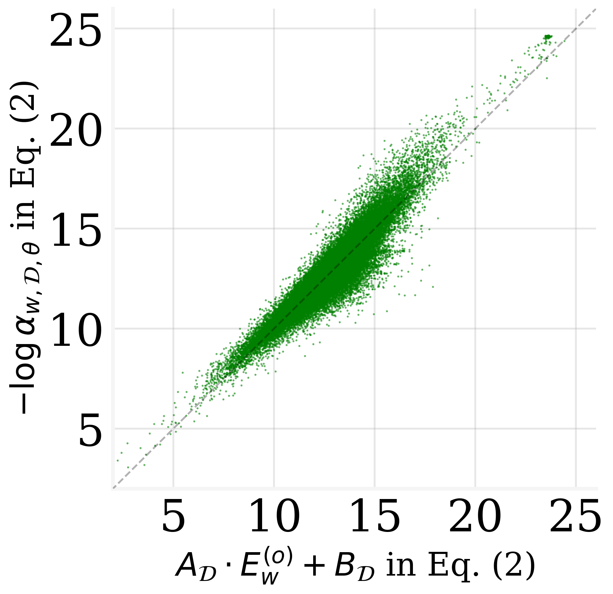
(b) GPT-J, 6B

Figure 2: The MLR results on GPT2 and GPT-J.

Additionally, we use such log-linear encoding to investigate how and when the word frequency information of the training corpus is encoded into the output embedding during the training process. In §5, we find that the frequency encoding occurs at the very early steps in the training dynamics of LMs, even earlier than an obvious convergence trend is observed.

The contribution of this paper can be summarized as:

• We find a log-linear correlation as an encoding of the output probability in the output embedding. That is, the output token probabilities are encoded in a particular common direction on the output embeddings log-linearly.

• Based on the findings, we edit the averaged output probabilities using such an encoding.

• Based on the findings, we remove dimensions with weak correlation to output probabilities without harm to the LMs.

• Based on the findings, we find that the LMs learn the token frequency in the training corpus at very early training steps.

Table 1: The goodnesses (Adj.$R^{2}$) of MLR of $-\log\alpha_{w,\mathcal{D},\theta}$ against the output($E^{(o)}_{w}$)/input($E^{(i)}_{w}$) embedding. Random Adj. $R^{2}$: The Adj.$R^{2}$ of normalized random vector against $E^{(o)}_{w}$. Parameter #: the number of LM parameters. Embedding tied: whether the output embedding is tied with the input embedding.

Model	GPT2	GPT2-XL	Pythia	GPT-J
Parameter #	137M	1.6B	2.8B	6B
Embedding tied	✓	✓	$-$	$-$
Random Adj.$R^{2}$	$0.001$	$0.000$	$0.001$	$0.000$
Adj.$R^{2}$ on $E^{(o)}_{w}$	$0.892$	$0.893$	$0.856$	$0.882$
Adj.$R^{2}$ on $E^{(i)}_{w}$	$(0.892)$	$(0.893)$	$0.814$	$0.658$

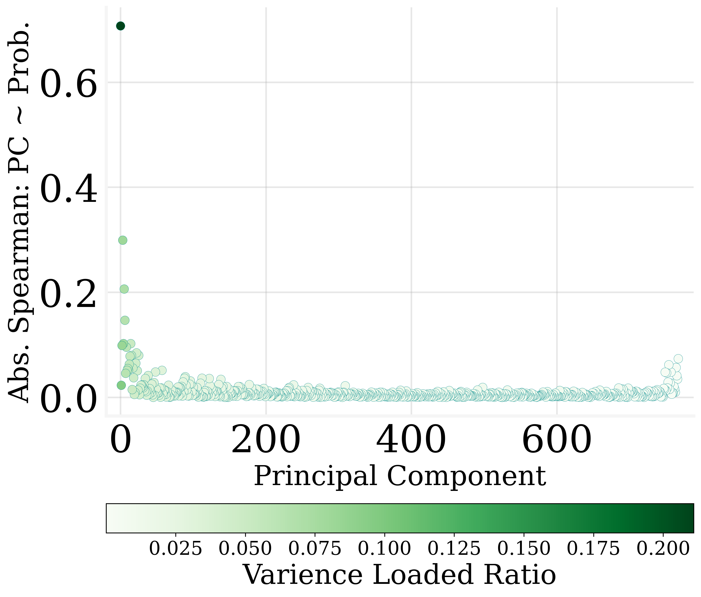
(a) GPT2, 137M, PCA

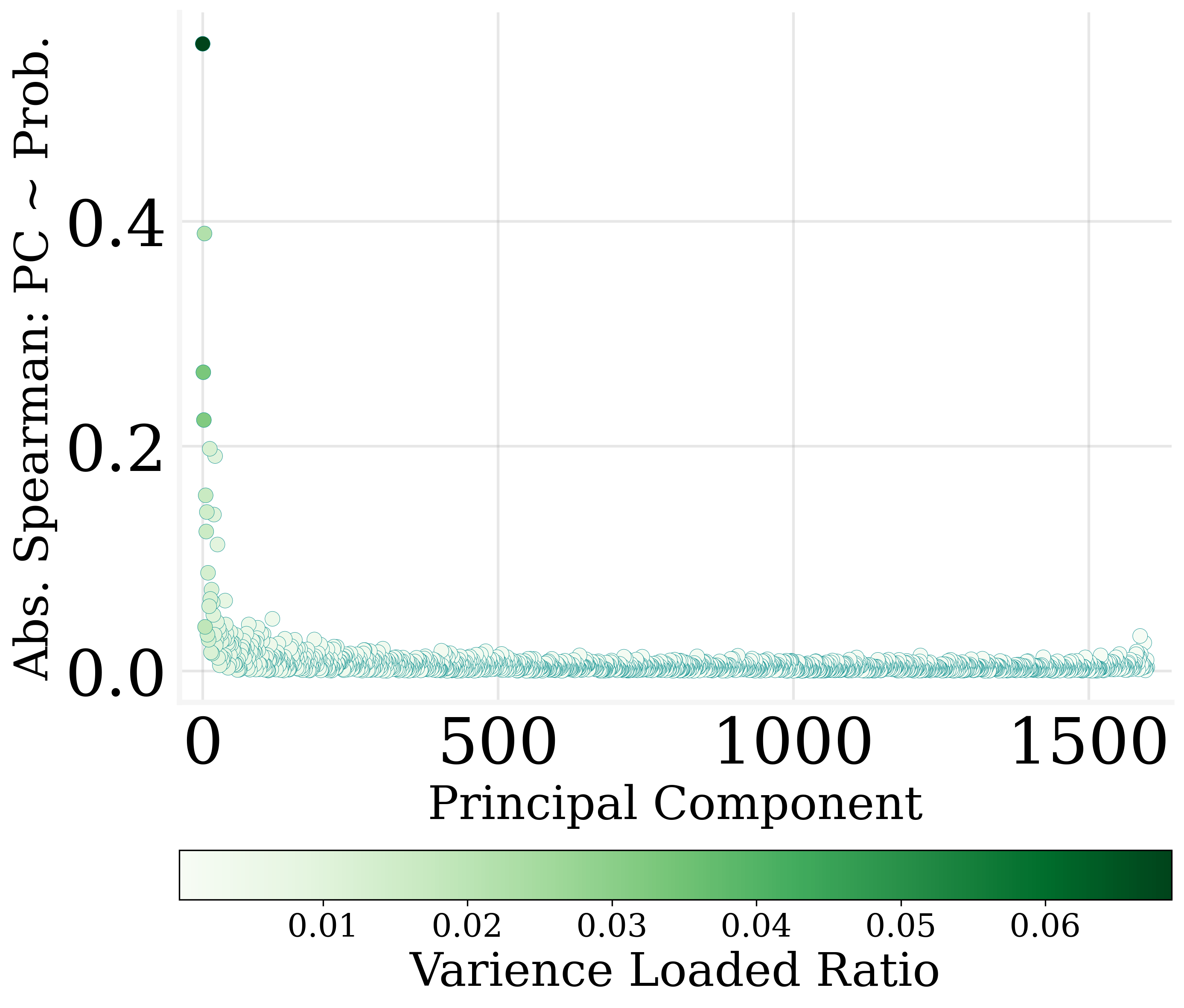
(b) GPT2-XL, 1.6B, PCA

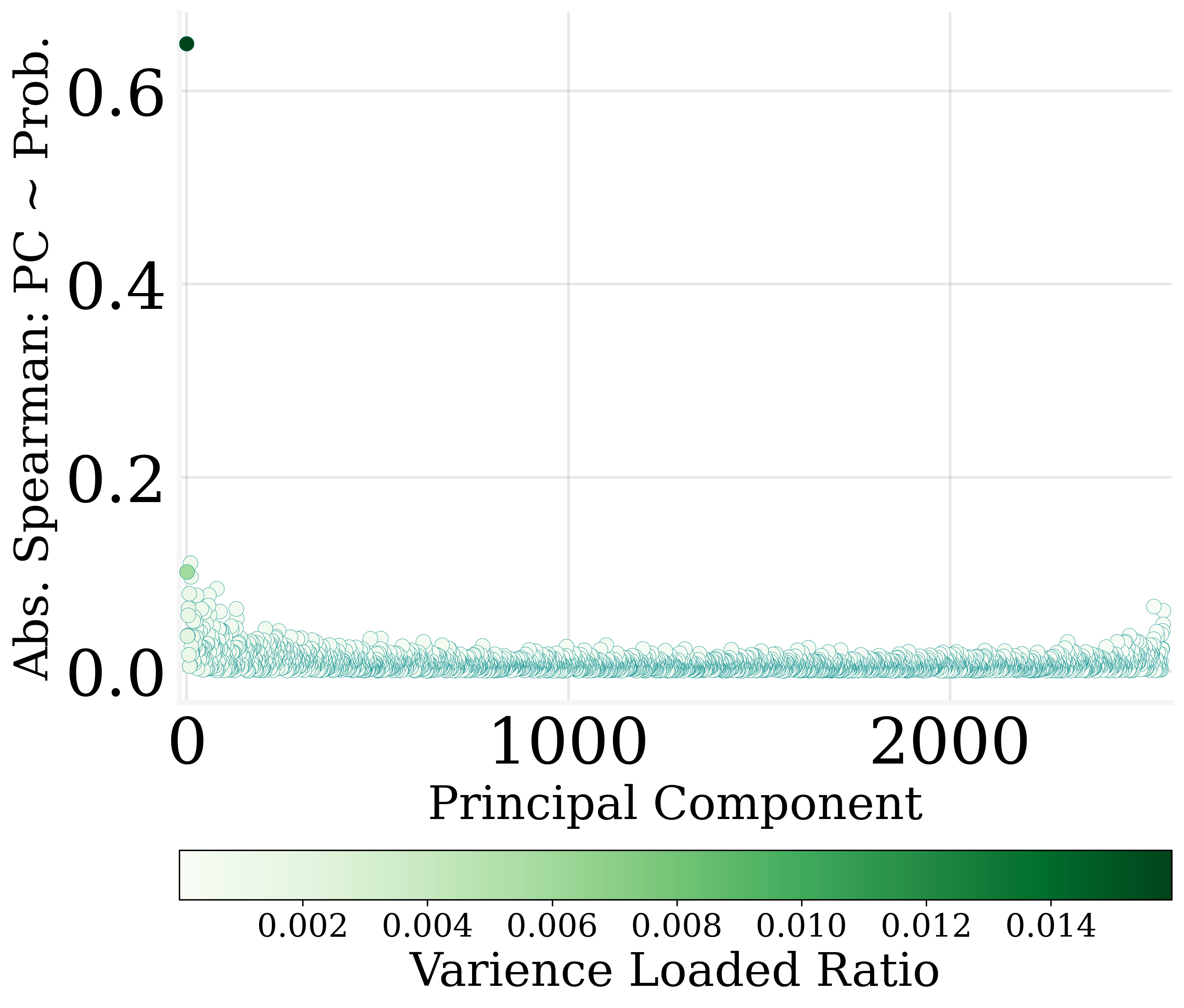
(c) Pythia, 2.8B, PCA

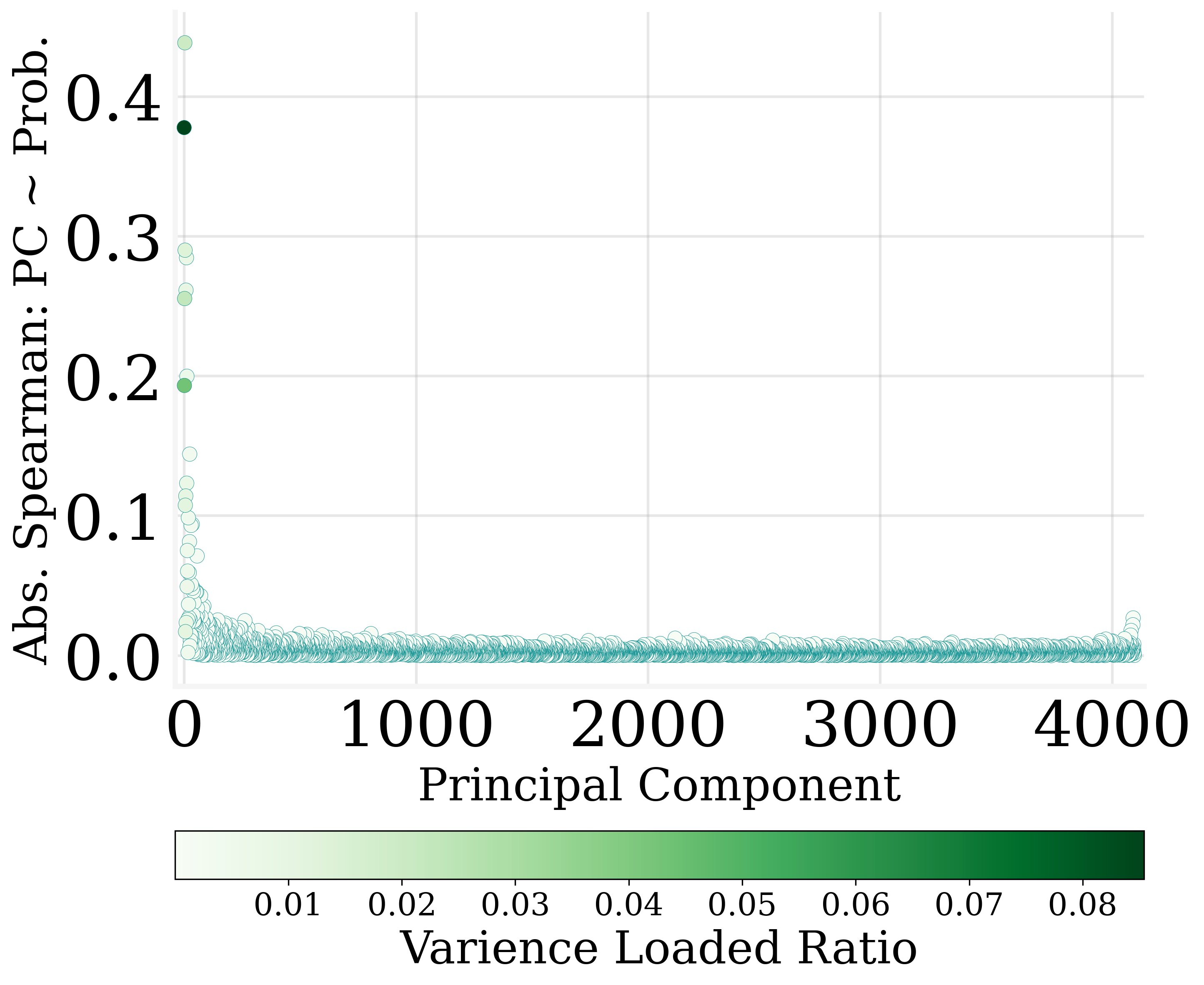
(d) GPT-J, 6B, PCA

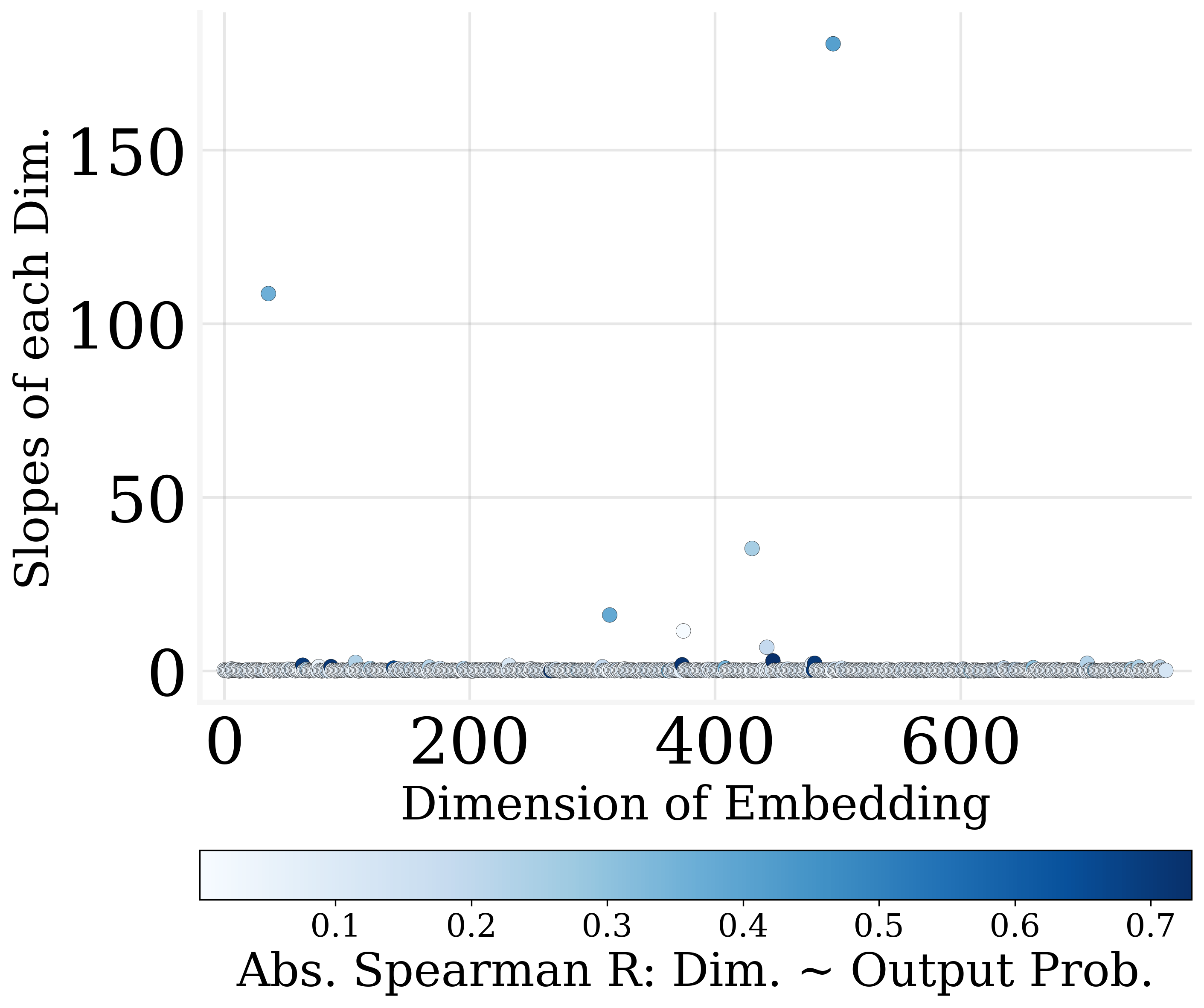
(e) GPT2, 137M, Original

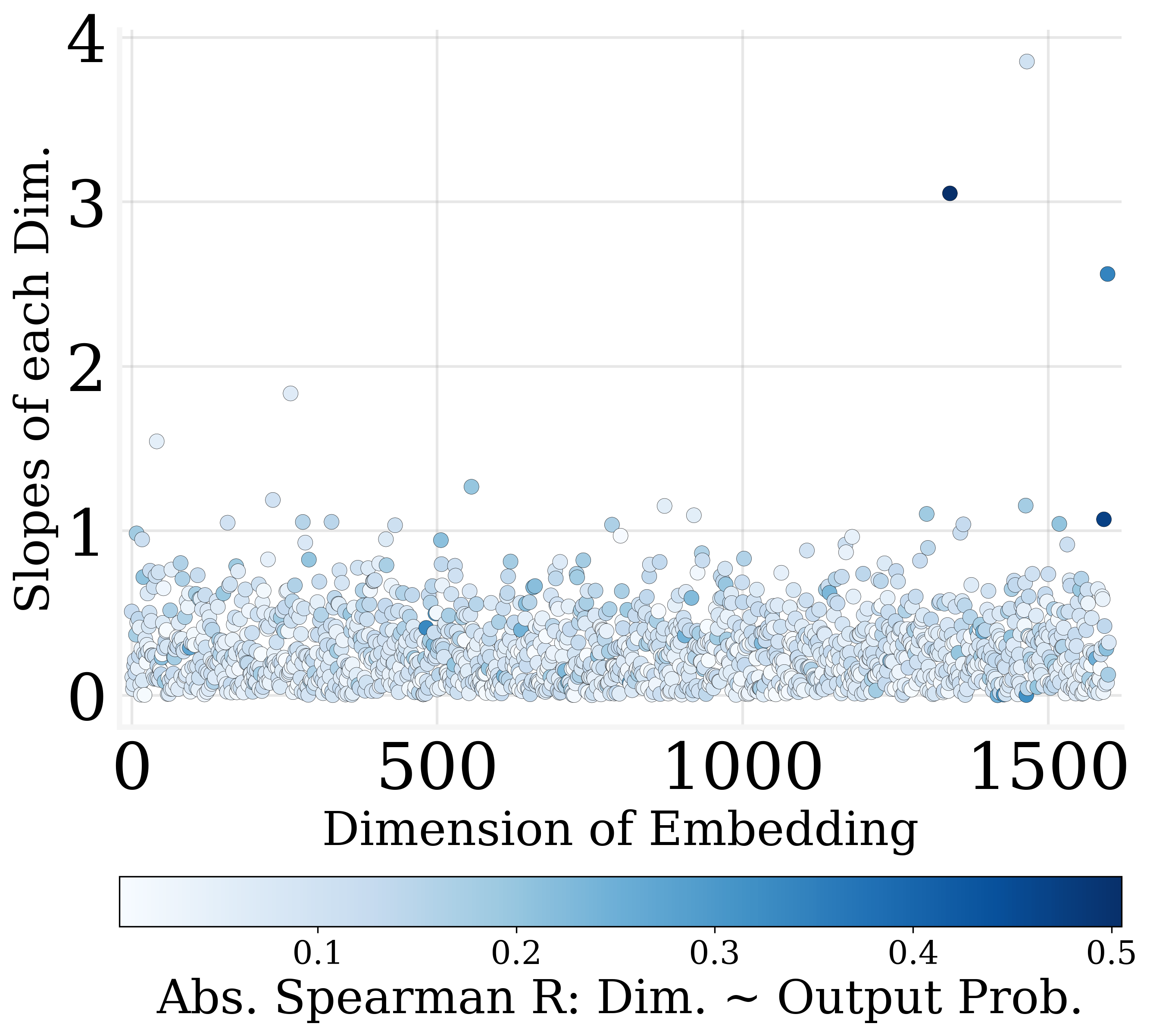
(f) GPT2-XL, 1.6B, Original

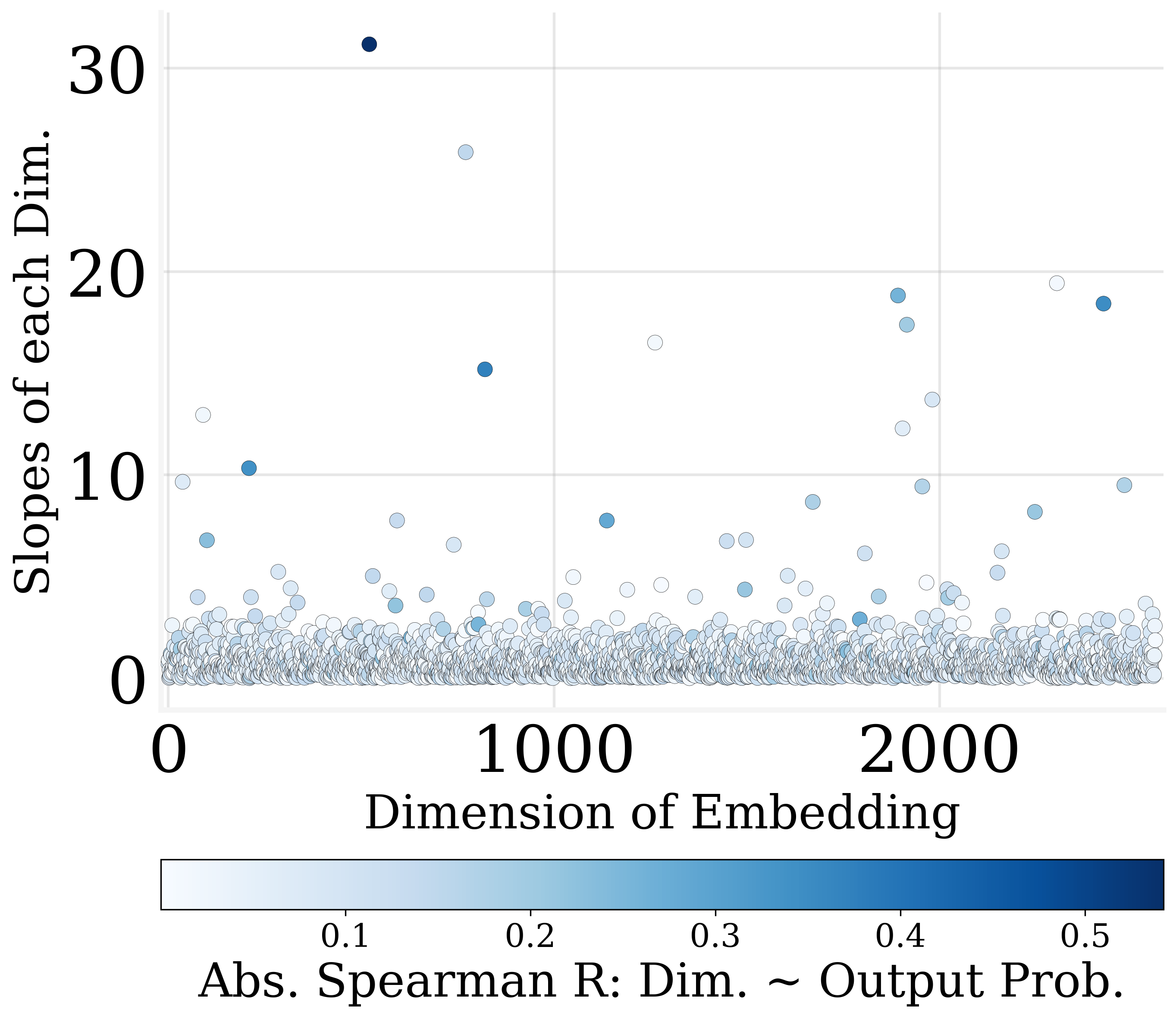
(g) Pythia, 2.8B, Original

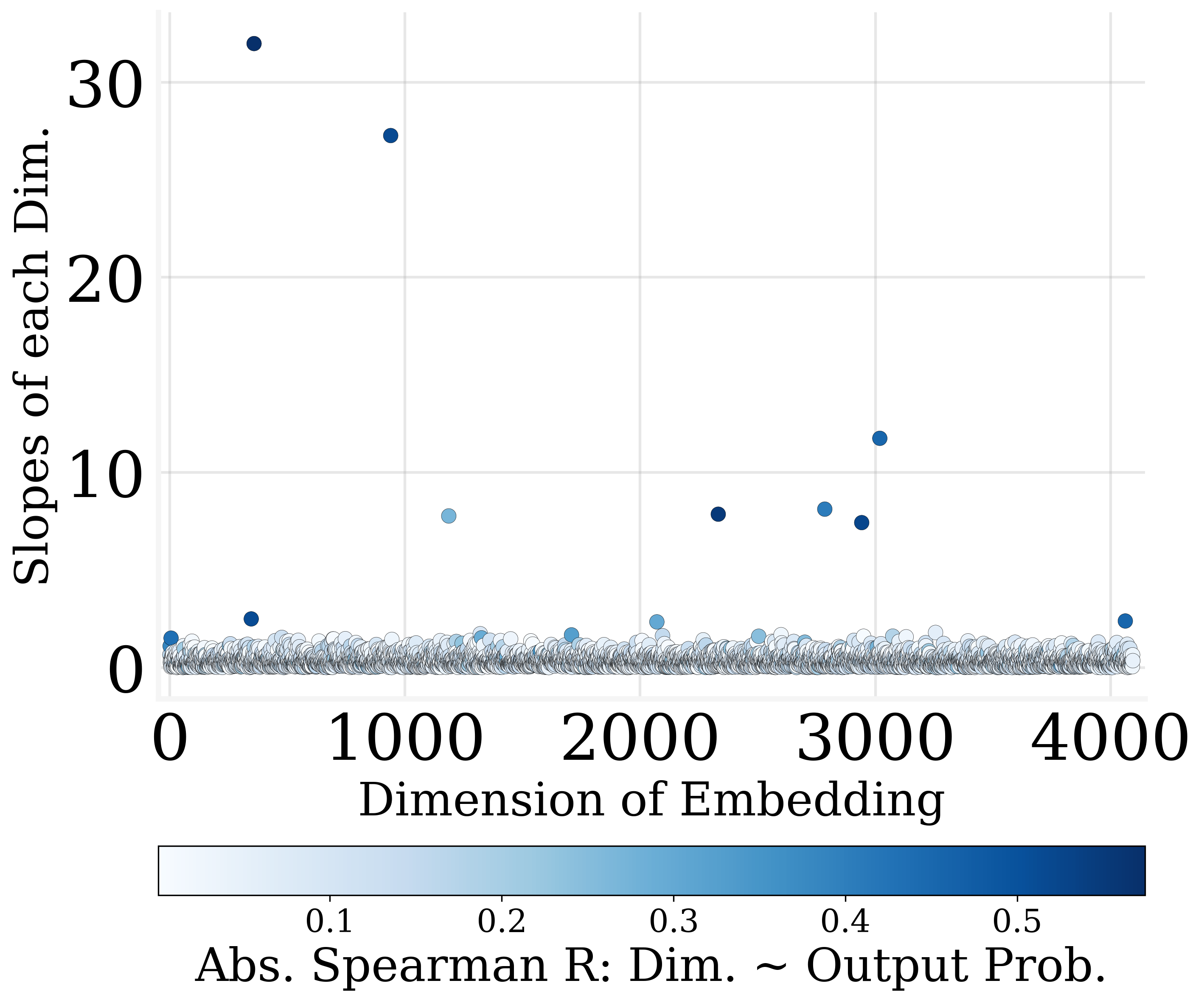
(h) GPT-J, 6B, Original

Figure 3: Only a few directions/dimensions of output embedding are strongly correlated to the output probabilities. (a-d): horizontal axis: the principle components of output embedding, vertical axis: absolute Spearman $r$ between the principle and the output probability distribution, color bar: the variance ratio loaded in the principle component; (e-h): horizontal axis: original dimensions, vertical axis: absolute MLR slopes between this dimension and the output probability distribution, color bar: the absolute Spearman correlations on the dimension.

2 Token Probability Encoding in Output Embedding

In this section, we preliminarily reveal how the output probabilities are encoded in the output embedding by derivation, then conduct simple numerical experiments to confirm it empirically.

Input: Language model $P_{\theta}(x)$ with output embedding $E^{(o)}$; Probability detecting dataset $\mathcal{D}$;
Token index to be edited $w$; Expected scale of the edited token’s probability $r$;
Editing amount allocation parameter $b$

Output: Updated LM $P_{\theta^{\prime}}(x)$

5

$\mathbf{\alpha}_{\mathcal{D},\theta}\leftarrow|\mathcal{D}|^{-1}\sum_{x\in\mathcal{D}}P_{\theta}(x)$ ;

  // Calculate the averaged probability distribution

6

$A_{\mathcal{D}},\mathcal{S}\leftarrow\mathrm{MLR}(-\log\mathbf{\alpha}_{\mathcal{D},\theta},E^{(o)})$ ;

  // Conduct the MLR, get the slope and confidence

7

$\Omega\leftarrow|A_{\mathcal{D}}|^{b}\times\mathcal{S}\times\||A_{\mathcal{D}}|^{b}\times\mathcal{S}\|_{1}^{-1}$ ;

  // Allocate the editing weight of dimensions

8

$E_{w}^{{}^{\prime}(o)}\leftarrow E_{w}^{(o)}-\log(r)\Omega\times A_{\mathcal{D}}^{-1}$ ;

  // Apply the editing to output embedding

9

10return Updated LM $P_{\theta^{\prime}}(x)$ with new output embedding $E_{w}^{{}^{\prime}(o)}$

2 $\mathbf{\alpha}_{\mathcal{D},\theta}\in\mathbb{R}^{|\mathbb{V}|}$: the output token probability distribution among the vocabulary; $|\mathcal{D}|$: the length of the probability detecting dataset; $\mathcal{S}$: the element-wise confidence ($p$-value) of the MLR;

Element-wise calculations: $(\cdot)\times(\cdot)$: multiplication; $(\cdot)^{p}$: $p$-th power; $|\cdot|$: absolute value.

Algorithm 1 Output token probability editing.

4 $\mathbf{\alpha}_{\mathcal{D},\theta}\in\mathbb{R}^{|\mathbb{V}|}$: the output token probability distribution among the vocabulary; $|\mathcal{D}|$: the length of the probability detecting dataset; $\mathcal{S}$: the element-wise confidence ($p$-value) of the MLR;

Element-wise calculations: $(\cdot)\times(\cdot)$: multiplication; $(\cdot)^{p}$: $p$-th power; $|\cdot|$: absolute value.

2.1 Mathematical Log-linear Form

Considering an LM parameterized by $\theta$ with vocabulary $\mathbb{V}$. Denoting the last hidden state w.r.t. input sequence $x$ as $h_{x}$, we can describe the output probability of token $w$ with an output embedding $E_{w}^{(o)}$ as:

$$P_{\theta}(w|x)=\frac{e^{E_{w}^{(o)}\cdot h_{x}}}{\sum_{i\in\mathbb{V}}e^{E_{i}^{(o)}\cdot h_{x}}},$$

we have:

$$-\log[P_{\theta}(w|x)]=-E_{w}^{(o)}\cdot h_{x}+\log[\sum_{i\in\mathbb{V}}e^{E_{i}^{(o)}\cdot h_{x}}].$$

When we calculate the averaged output token probability $\alpha_{w,\mathcal{D},\theta}=\mathbb{E}_{x\in\mathcal{D}}[P_{\theta}(w|x)]$ of token $w$ on a dataset $\mathcal{D}$ (detecting dataset):

$$\begin{split}&-\log\alpha_{w,\mathcal{D},\theta}\approx\mathbb{E}_{x\in\mathcal{D}}[-\log[P_{\theta}(w|x)]]\\ =&-\mathbb{E}_{x\in\mathcal{D}}[E_{w}^{(o)}\cdot h_{x}]+\mathbb{E}_{x\in\mathcal{D}}[\log(\sum_{i\in\mathbb{V}}e^{E_{i}^{(o)}\cdot h_{x}})]\\ =&-E_{w}^{(o)}\cdot\mathbb{E}_{x\in\mathcal{D}}[h_{x}^{(o)}]+\mathbb{E}_{x\in\mathcal{D}}[\log(\sum_{i\in\mathbb{V}}e^{E_{i}^{(o)}\cdot h_{x}})].\end{split}$$ (1)

We make a local linear approximation in the approximately equal sign, while we confirm it is precise when the output logits are concentrated in Appendix B.2. Notice that if the LM head is biased, the bias term can be re-constructed equally by fixing one dimension of $h_{x}$ to $1$, w.l.o.g.

We denote $A_{\mathcal{D}}=-\mathbb{E}_{x\in\mathcal{D}}[h_{x}]$, and $B_{\mathcal{D}}=\mathbb{E}_{x\in\mathcal{D}}[\log(\sum_{i\in\mathbb{V}}e^{E_{i}^{(o)}\cdot h_{x}})]$. Here we do another approximation that the $B_{\mathcal{D}}$ is independent to $E_{w}^{(o)}$. This approximation is precise when the logits of the output token $w$ are small, and the vocabulary size $|\mathbb{V}|$ is large. Then, we get an approximated log-linear form between the $\alpha_{w,\mathcal{D},\theta}$ and the $E_{w}^{(o)}$:

$$-\log\alpha_{w,\mathcal{D},\theta}\approx A_{\mathcal{D}}\cdot E_{w}^{(o)}+B_{\mathcal{D}}.$$ (2)

As a special case, we consider a fixed-to-one dimension in $h_{x}$ (also in $A_{\mathcal{D}}$) for a biased LM head, where the bias re-constructed in $E_{w}^{(o)}$ becomes a linear factor of $-\log\alpha_{w,\mathcal{D},\theta}$ with slope $1$.

With such a derivation, we find that the phenomenon shown in Fig. 1 is the nature of $\mathrm{softmax}$ output head if it has plenty of classification categories, small and concentrated logits to make the approximations numerically accurate. LMs have a very wide output space and undergo regularized training, which makes LMs meet the requirements to have an accurate log-linear correlation between output probabilities and output embeddings. That is, the output probabilities are encoded within a common direction of output embedding.

2.2 Empirical Confirmation

We conduct experiments to prove our derivation in Eq. 2 empirically correct. First, following Kobayashi et al. (2023), we calculate the averaged output probabilities on an 8192-length sample of shuffled WikiDpr dataset Karpukhin et al. (2020). In detail, we input the sampled data points into the model, and average the output probability distribution among every time step of every input sequence as the token probability distribution of the dataset (see Appendix B.1). Then, we conduct MLR to fit the $A_{\mathcal{D}}$ and the $B_{\mathcal{D}}$.

We run such experiment on GPT2, GPT2-XL Radford et al. (2019), Pythia 2.8B Biderman et al. (2023), and GPT-J Wang and Komatsuzaki (2021). The fitting results are shown in Fig. 2, where good fittings are observed. We also list the adjusted $R^{2}$ i.e. the goodness of fitting in Table 1. Surprisingly, both input and output embeddings have strong correlations with the token probabilities.

More interestingly, as shown in Fig. 3, we find that only the top principal components and a few dimensions in the output embedding are highly correlated to the output token probabilities. In detail, we calculate the absolute Spearman $r$ between the output embedding’s sorted principle components / original dimensions against the output probabilities, and we find that the overwhelming majority of both kinds of dimensions have poor correlations with the output probabilities.

3 Token Probability Editing on Output Embeddings

Our findings suggest that the output probabilities are encoded in a common direction in the output embeddings. So we try to edit the token probabilities by modifying a small portion of dimensions in the output embeddings following such a direction, as an application and further empirical proof of the findings.

3.1 Algorithm

Based on the fact that the output probabilities are log-linearly encoded in a direction on the output embedding, and the correlation strengths significantly vary among dimensions, we propose an output probability editing algorithm as shown in Algorithm 1. We first calculate an output probability distribution $\mathbf{\alpha}_{\mathcal{D},\theta}$ on a corpus $\mathcal{D}$ and conduct MLR to calculate the $A_{\mathcal{D}}$ and the confidence ($p$-value) $\mathcal{S}$ of each element of the common encoding. Then we assign an editing weight $\Omega$ to every dimension in the embedding vector based on the significance of its correlation to the output probabilities, as shown in line 3 of Algorithm 1. We allocate more editing amount to stronger correlations to obtain smaller and more accurate editing. Given the token index to be edited and the expected editing scale, we calculate the detailed editing amount on each dimension and update it as shown in line 4 of Algorithm 1.

As calculation costs, such an editing algorithm only needs a detect set $\mathcal{D}$ and a feed-forward process to calculate the $A_{\mathcal{D}}$ and $\mathcal{S}$. We are about to prove that it is stable for the size of $\mathcal{D}$ and consistently precise.

Table 2: Main results on the evaluation of Algorithm 1. Unedited: the baseline without any editing. Random: the baseline with a random $A_{\mathcal{D}}$. Shuffled: the baseline with a shuffled $A_{\mathcal{D}}$ from the origin one. It is difficult to conduct MAUVE experiments of GPT-J on such a repeating scale due to the enormous computational costs. $b$: the editing amount allocation parameter in Algorithm 1. Fine-grained results are presented in the Appendix D.

	Emb. Tied	$b$	Reliability	Generalization		Specificity
			$e_{local}\downarrow$	$e_{id}\downarrow$	$e_{ood}\downarrow$	$d_{KL}^{r}\times 10^{-7}\downarrow$	MAUVE$\uparrow$
unedited	$-$	$-$	${1.10}_{1.06}$	${1.10}_{1.06}$	${1.10}_{1.06}$	${0.00}_{0.00}$	${1.00}_{0.00}$
137M, random	✓	2	${1.33}_{1.28}$	${1.33}_{1.28}$	${1.29}_{1.24}$	${2.31}_{1.02}$	${0.96}_{0.01}$
137M, shuffled	✓	2	${1.18}_{1.07}$	${1.18}_{1.08}$	${1.18}_{1.08}$	${1.64}_{0.48}$	${0.96}_{0.01}$
137M	✓	2	${0.19}_{0.30}$	${0.20}_{0.32}$	${0.15}_{0.28}$	${9.51}_{5.87}$	${0.96}_{0.01}$
1.6B	✓	2	${0.64}_{0.67}$	${0.61}_{0.65}$	${0.65}_{0.63}$	${1.51}_{3.66}$	${0.91}_{0.17}$
6B	$-$	5	${0.31}_{0.43}$	${0.25}_{0.39}$	${0.10}_{0.12}$	${3.64}_{14.65}$	$-$

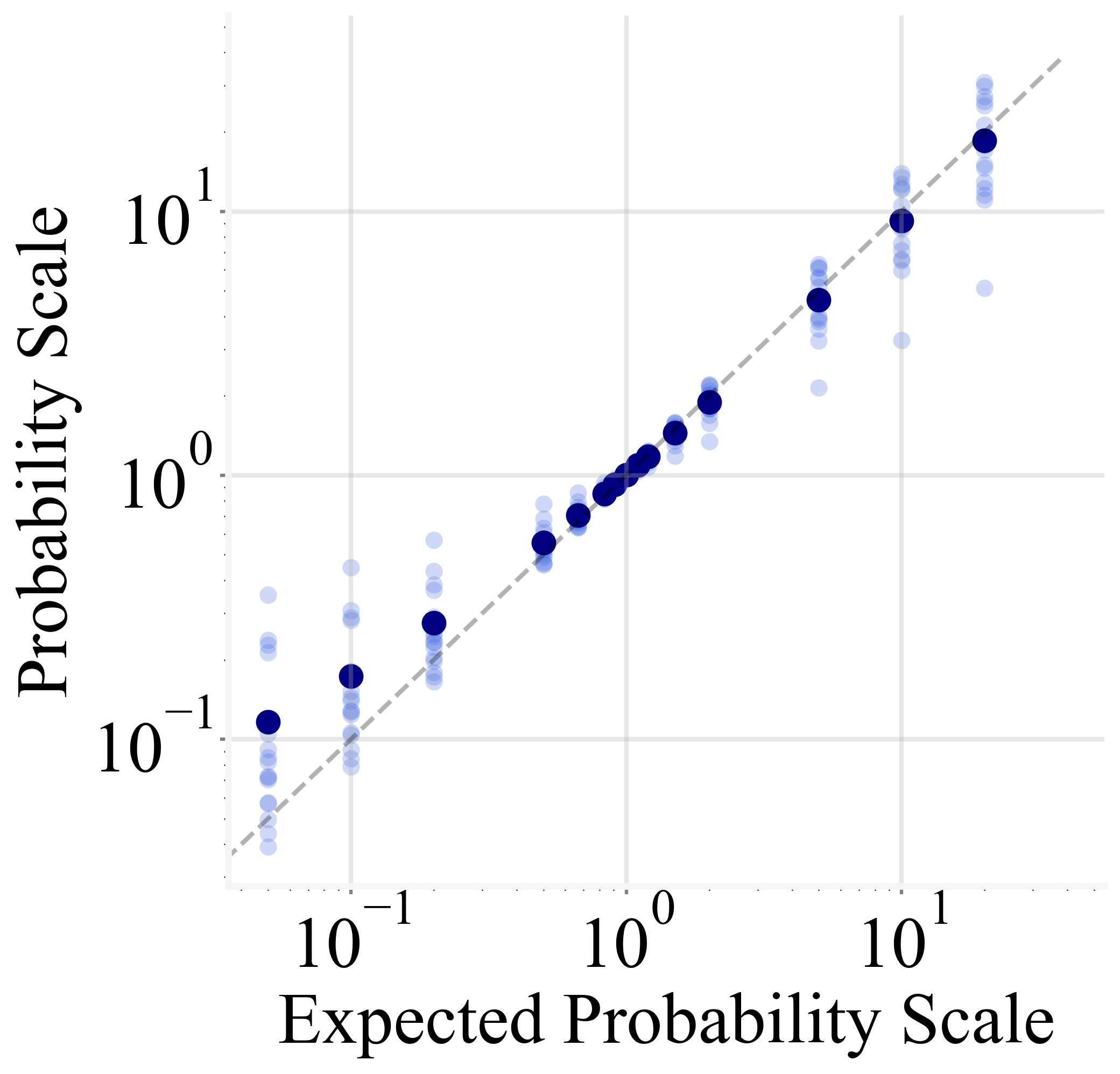
(a) GPT2, 137M

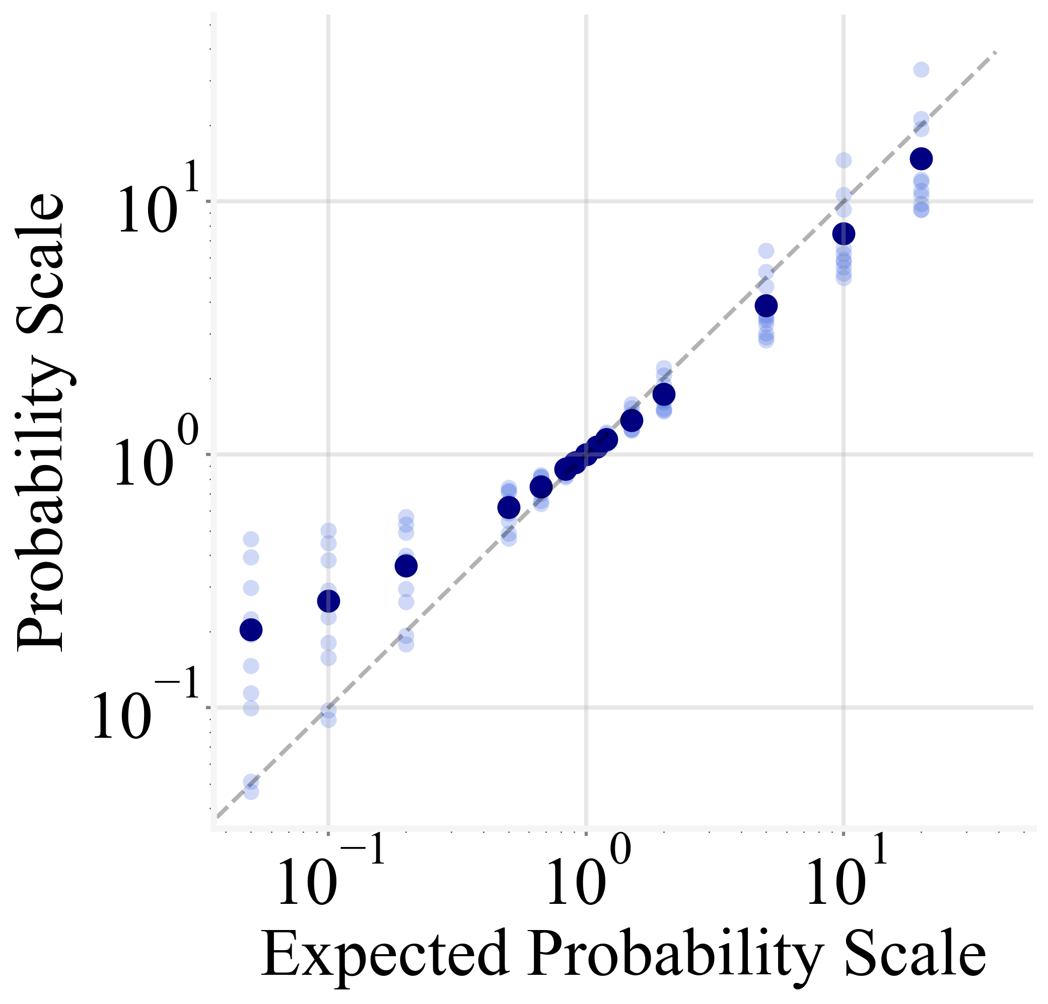
(b) GPT-J, 6B

Figure 4: The expected probability scales against the actually edited scales measured in the edited LMs.

3.2 Experiment Settings

We use the same detect dataset $\mathcal{D}$ as in §2, and a set of scales of {1, 1.1, 1.2, 1.5, 2, 5, 10, 20} for both scaling up and down. We randomly select 10 tokens to be edited and conduct experiments on GPT2, GPT2-XL, and GPT-J.

Metrics.

We use 3 metrics to test the algorithm.

• Scale error $e$: To describe the precision of the probability editing, given the expected editing scale $r$ and the actual measured edited scale $\hat{r}$ on a test dataset, the scale error is calculated as $e=|\ln(r)-\ln(\hat{r})|$.

• KL divergence on the unedited token $d_{KL}^{r}$: To investigate the side effect on the unedited tokens, we calculate KL divergence between the probability distribution before and after editing on the unedited tokens.

• MAUVE: To investigate the side effect on text generation, we generate a set of sentences from the edited model, then calculate the MAUVE with the generated set from the unedited model (see Appendix B.3).

Evaluations.

Following the widely-used aspects of model editing evaluations Yao et al. (2023), we define our evaluations as:

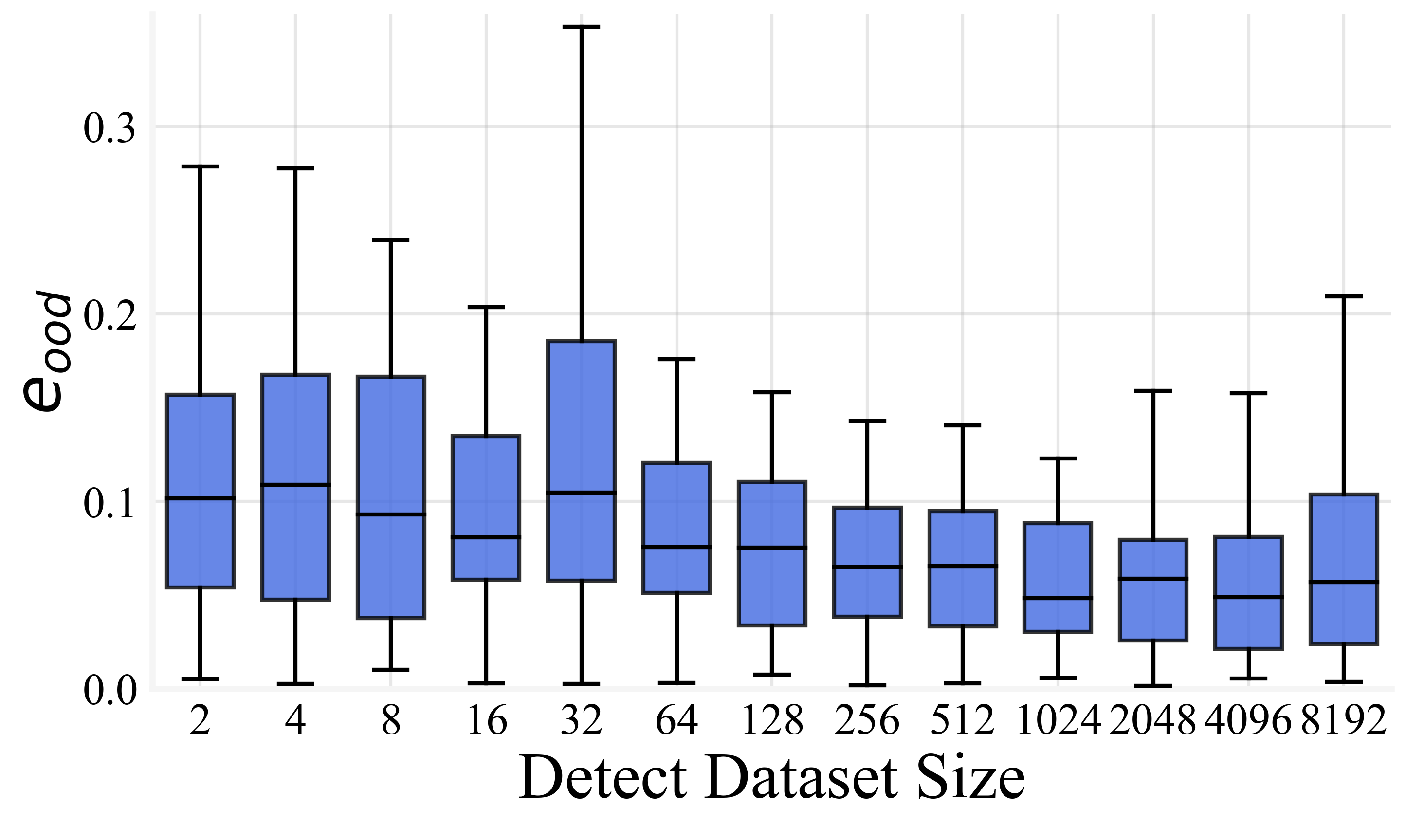
Figure 5: The $e_{ood}$ on detect datasets with various numbers of sentence (averaged token per sentence $\approx 134$).

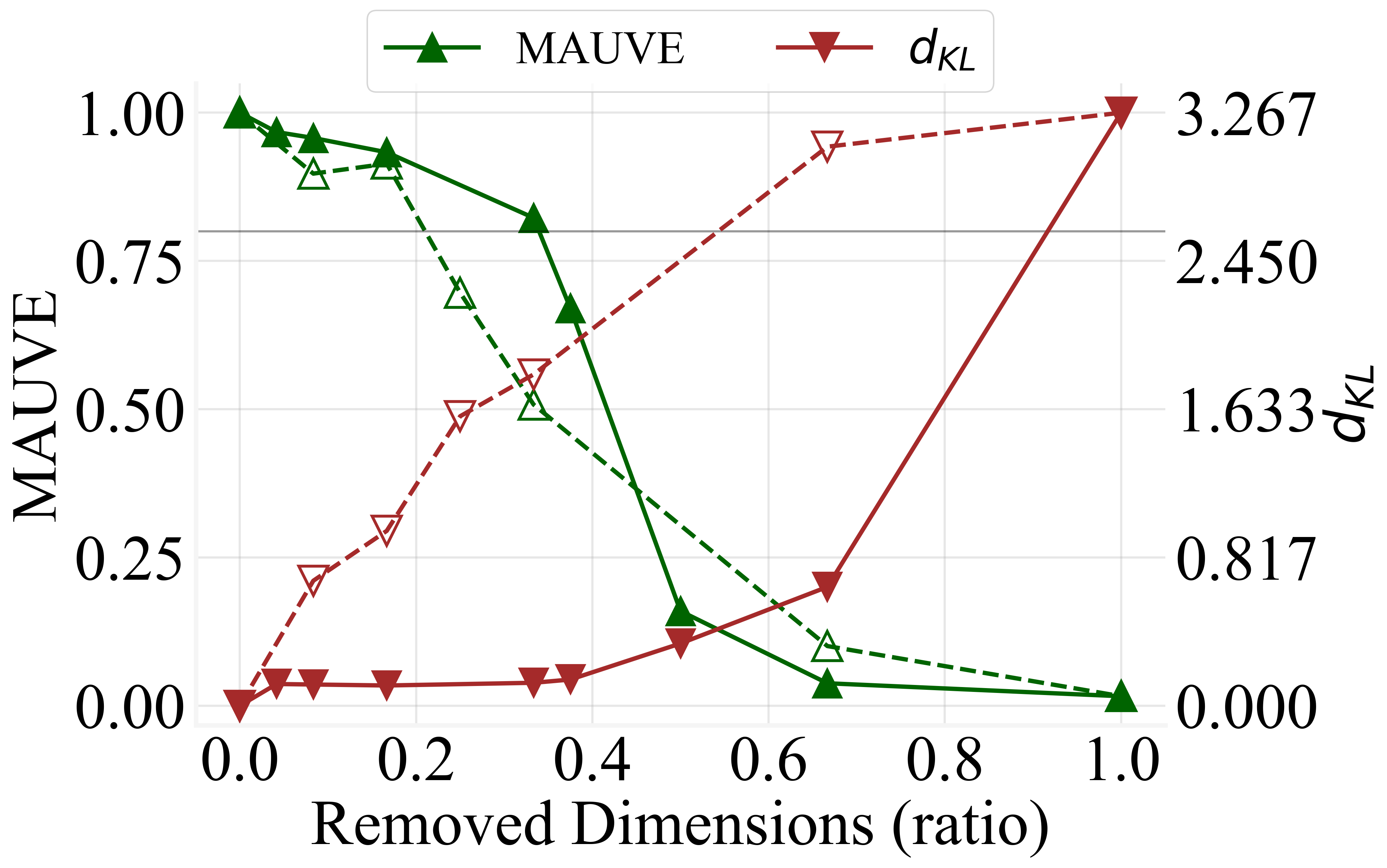
(a) GPT2, 137M, dim=768, tied

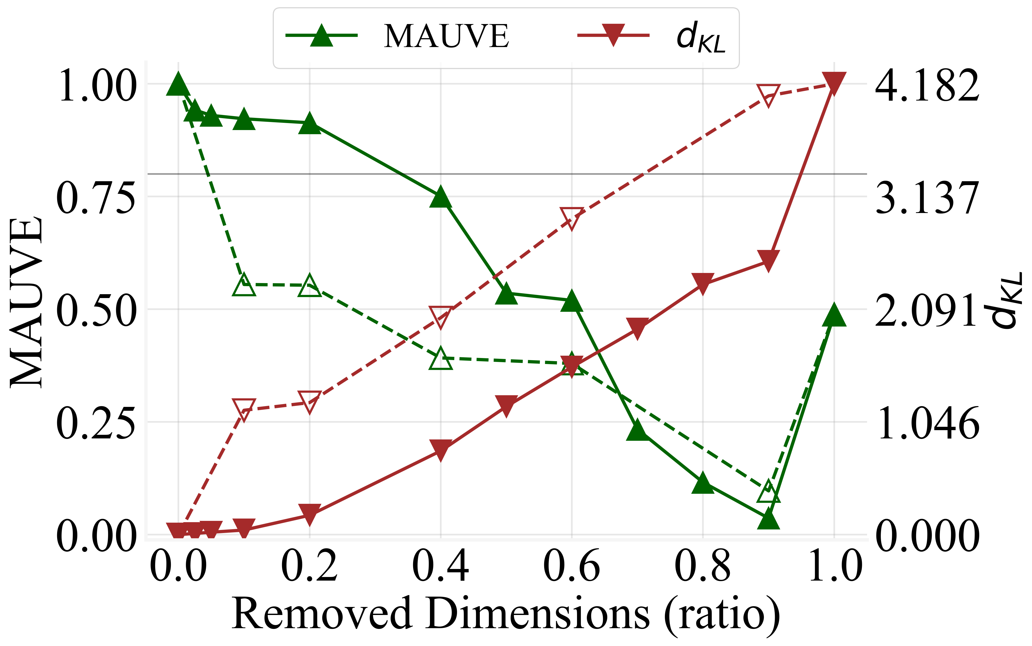
(b) Pythia, 2.8B, dim=2560

(c) GPT-J, 6B, dim=4096

Figure 6: The MAUVE$(\uparrow)$ and KL divergence$(\downarrow)$ of output token probability distribution $d_{KL}$ against original distributions w.r.t. the dimension removing ratio on the output embedding. Solid curves: results of removing dimensions from the least important ones to the most important ones; Dashed curves: adversarial controlling experiment, removing dimensions reversely.

• Reliability: The local effectiveness of the editing method. We use $e_{local}$, the scale error on the detect dataset $\mathcal{D}$.

• Generalization: The global effectiveness of the editing method. We set multi-level generalization evaluations to ensure that the conclusions we obtain are the generalizable essence of the model: (i). the scale error on the other 8192 samples of WikiDpr as the In-domain Scale Error $e_{id}$; and (ii). the scale error on 2048 samples of BookCorpus Zhu et al. (2015) as the Out-of-domain Scale Error $e_{ood}$.

• Specificity: The non-harmfulness to unedited part. We use two settings for this evaluation: (i). the averaged $d_{KL}^{r}$ on the three data samples (detect set, in-domain, out-of-domain), and (ii). the aforementioned MAUVE.

3.3 Results

The main statistical evaluation results are shown in Table 2, where we can get a basic intuition that the Algorithm 1 is accurate and generalizable, even on the out-of-domain data. Especially, despite the embedding tying in GPT2 and GPT2-XL, such an editing algorithm is still accurate and harmless, which demonstrates that the log-linear probability encoding is orthogonal to the possible semantical encoding in the output and also input embedding.

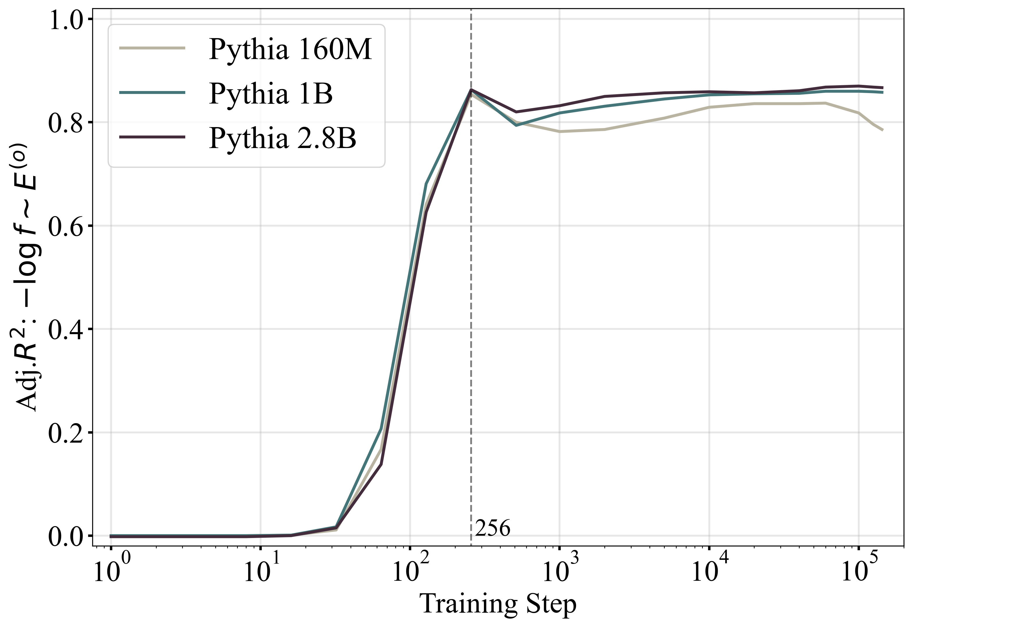
(a)

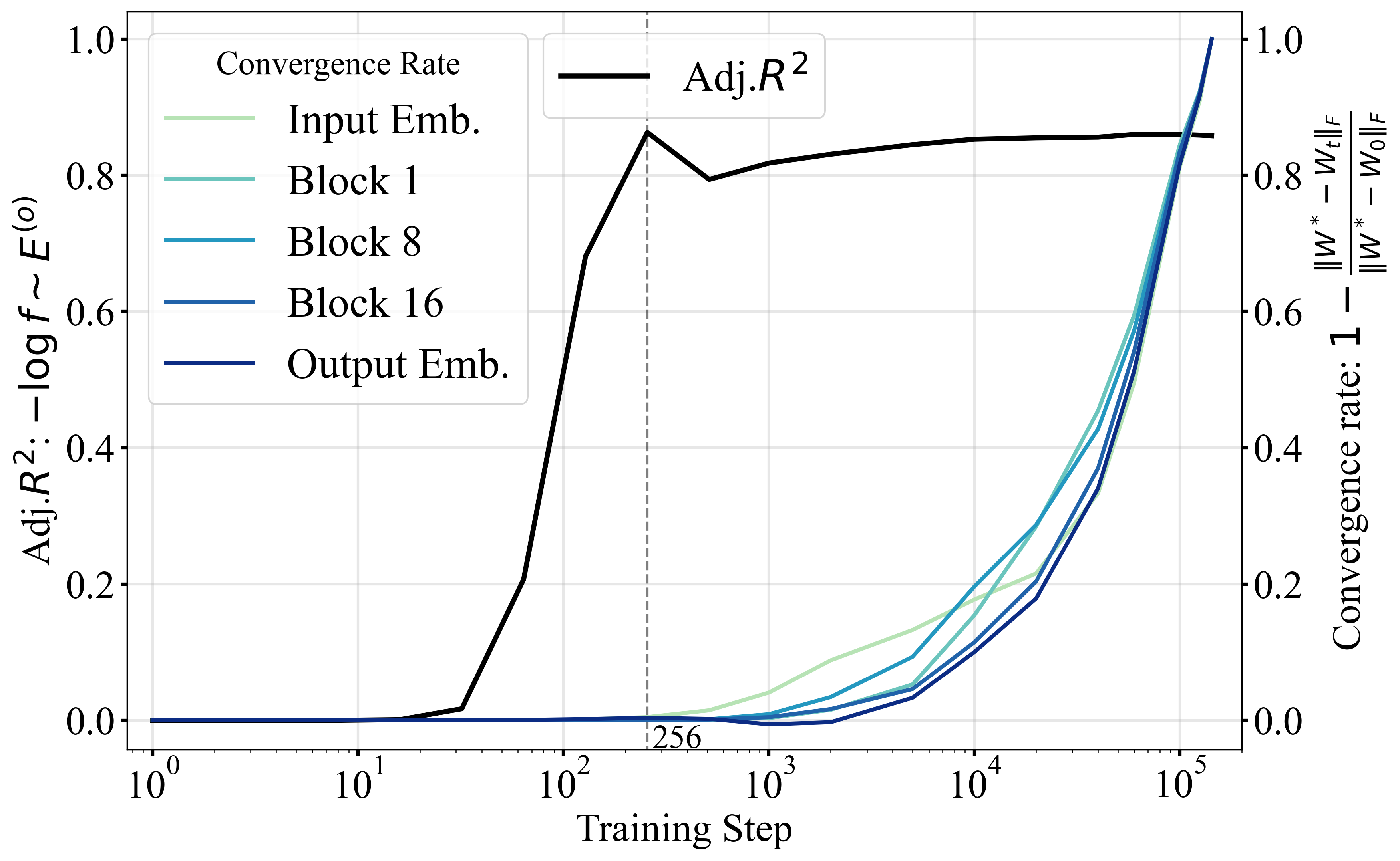
(b)

Figure 7: The training dynamics of Pythia. Left: the MLR goodness (adjusted $R^{2}$) of the negative logarithm of corpus frequency against the output embedding. Right: on the Pythia-1B, the MLR goodness in the left figure, and the convergence rate of various representative blocks. Notice the horizontal axis is logarithmically scaled.

Wide-scale stable: Large-scaled probability editing is supported by a global log-linear pattern.

The correlation of actually edited scales of token probability against the expected scales is shown in Fig. 4. The editing remains accurate even on a large scale of up to 20x. This indicates that the algorithm and the log-linear encoding are wide-ranging, not only locally effective, i.e. the log-linear encoding is a widely stable common essence.

Few-shot generalizable: Encoding remains distinct even by an $A_{\mathcal{D}}$ estimated by few-shot corpus.

Instead of using the 8192 examples for the detecting dataset $\mathcal{D}$, we try various numbers of examples to test the generalization of the encoding on GPT2. As shown in Fig. 5, we find that even 2 examples can produce a distinct averaged probability distribution for precise probability editing. This result strengthens the significance and generalization of our findings, that is, effective statistical patterns can be found in a small set of samples.

These results demonstrate the wide-scale stability and generalization of our algorithm, while also reflecting the same attributes of token probability encoding in output embedding. We can confirm that such log-linear encoding of token probabilities is an inherent attribute of output embedding, which (1). has wide-scale linearity, allowing a large-scaling probability editing, and (2). is common among tokens, so only a small number of samples are needed to find an accurate encoding. By our editing experiments, the properties of probability encoding are strengthened.

4 Removing Dimensions with Weak Probability Encoding

Moreover, based on the sparsity of probability encoding as shown in Fig. 3, we can infer that a large number of dimensions are less effective for causal language modeling, where the expected role of the LM head is basically only to predict probabilities. So we try to reduce the less related dimensions towards a lightweight output head.

4.1 Method & Experiment Settings

First, we assign a weight of importance (or, saliency) to each dimension of output embedding from the aforementioned absolute MLR slopes as shown in (e-h) of Fig. 3. Then, we remove the dimensions in ascending order of such weight, i.e. we remove the less important dimension early. In detail, as a prototype setting in the laboratory, we only zero out the dimensions in the embedding matrix, while the dimensions of the attention mapping matrix, the feed-forward layer, and the dimensions of the last hidden state corresponding to the removed dimensions can also be removed equally.

Experiment Settings.

We use the same MLR settings as §2 on GPT2, Pythia 2.8B, and GPT-J. As metrics, we test the MAUVE of the pruned model similarly to §3.2, and test the KL divergence of the averaged probability distribution against the original model on the out-of-domain dataset mentioned before. As an adversarial controlling experiment, we remove dimensions in descending order of importance, i.e. we remove the more important dimension early, reverse to the original settings.

4.2 Result

The results are shown in Fig. 6. With the ascending removing order (the positive experiment, solid curve), at the beginning of the removal, both metrics deteriorate slightly until around 50% of the dimensions are removed. Regarding $\mathrm{MAUVE}>0.80$ as a threshold, we can confirm that $30\%\sim 40\%$ of the dimensions in the output embedding can be removed without significant impairment of the causal language modeling ability of LMs. In contrast, in the adversarial experiment with a descending removing style (dashed curve), both metrics deteriorate sharply at the beginning of removing. Such results suggest that the weights from the MLR are faithful importance metrics.

Noticeably, our method also works on the tied models, i.e. removing unnecessary dimensions concurrently from the input embedding and the output embedding, the causal language modeling ability of the LM remains at a considerable level.

Consistent with previous works Kovaleva et al. (2021); Timkey and van Schijndel (2021); Gordon et al. (2020), our results identify the difference in the importance among the dimensions of the output embedding. Moreover, we confirm that the MLR results of the log-linear correlation are a good metric of importance, i.e. saliency score. This can be a new paradigm of saliency if a direct one-step statistical model can be found between the features and the model output.

5 Output Embedding Learns Corpus Frequency in Early Training Steps

Additionally, the findings in this paper inspire us to utilize such log-linear correlation for detecting the encoding of corpus token frequency in the output embedding during the training. Intuitively, since the model can refract overall output probability distribution in the output embedding matrix, it should be forced to produce the same output distribution with the corpus token frequency by the training objective. Therefore, when a log-linear encoding of token frequency of the training corpus is observed in the output embedding, we can confirm that the output embedding learns the token frequency information of the corpus.

We use the Pythia suite Biderman et al. (2023), where sequences of the model intermediate training checkpoints are saved. We estimate the token frequencies of the training corpus Pile Gao et al. (2020); Biderman et al. (2022) by sampling 14.3B tokens, then conduct MLR on the negative logarithm of the token frequencies w.r.t. the output embeddings on each training checkpoint. The results are shown in the left part of Fig. 7, where we can confirm an effective encoding since the very early steps of the training process, and larger models have slightly better fitting goodness but almost no difference in the timing of emergence.

Moreover, we want to know whether such a phenomenon is a subsidiary effect of the convergence of the parameters. We use the convergence rate following the Chen et al. (2022) to describe the actual training completion: denoting the trained parameter matrix as $\theta^{*}$, the initialized parameter matrix as $\theta_{0}$, and the parameter matrix at step $t$ as $\theta_{t}$, the convergence rate at step $t$ can be written as $(1-\|\theta^{*}-\theta_{t}\|_{F}/\|\theta^{*}-\theta_{0}\|_{F})$. We visualize the convergence rate of the input and output embeddings and the query-key-value mapping matrix of the multi-head attention blocks on Pythia-1B, as shown in the right part of Fig. 7. We find that the log-linear correlation occurs even earlier than an obvious convergence trend is observed by the convergence rate. Or rather, the appearance of such correlation happens to be the starting point of the convergence process of the model. We infer that the output embedding should learn the coarse-grained output pattern earlier than the semantics details.

Additionally, we initially find that each layer of the transformer appears to have a uniform convergence curve, instead of an obvious deeper-slower pattern found by Chen et al. (2022). Especially, the input embedding and output embedding have almost overlapping training curves. We speculate that this is the effect of such full-residual connection networks, which makes the layering of the network inconspicuous during the gradient descent.

6 Conclusion and Discussion

Conclusion.

In this paper, based on the observation of a linear-like correlation between the output token probability and the output token embeddings shown in Fig. 1, we derive an approximate log-linear correlation from the nature of $\mathrm{softmax}$ output head with a large output space and concentrated output value, i.e. the output token probabilities are encoded in a common direction of output embeddings. Along such encoding direction, we edit the token probabilities with high accuracy, stability, and generalizability. Then, based on the sparsity of the encoding, we can distinguish the contributions of dimensions for the output probability of the model. We try removing the determined non-contributing dimensions, and no critical deterioration is found. Finally, based on the findings, we find that the LMs catch the token frequency in training data at very early steps in the training process log-linearly, even earlier than an obvious convergence trend is observed. This paper reveals the inner mechanism of LM heads on the causal language modeling task and helps understand the global principles and training dynamics of LMs.

Comparing to previous works.

Previous work about analyzing LM heads was conducted by Kobayashi et al. (2023), where a correlation between the output token probability and bias term in the LM head was found. They declared that the bias term is a projection to extract the probability from the output embedding, but no more discussion about the embedding matrix, which is the major component of the LM head. Making up for their work is one of the original motivations for our work. More discussions about related works can be found in Appendix A.

Demonstrations towards application.

Our output probabilities editing algorithm on the LM head reveals the possibility of model editing on only the output probability rather than in the hidden states or the lower layers Dai et al. (2022); Meng et al. (2022), which is more concise, and easy to explain. Some global toxicity generation Gehman et al. (2020), or biases in some application scenario Fei et al. (2023) can be suppressed by such a method, but as we will mention in the Limitations, it is elegant but not engineering-oriented. Moreover, the dimension compression method in this paper can be an easy-to-use and harmless inference-time acceleration. Notice that we have a supervising on such dimension compression by the MLR slopes, so it can be more accurate than the previous random or unsupervised pruning Gordon et al. (2020).

Towards a new saliency score of output embeddings.

Saliency score Zhao et al. (2024); Sun et al. (2021) is to weight a component (feature or parameter) in a deep learning model by its importance. In this paper, we find that the log-linear token probability encoding works like a saliency score towards the output embedding. We build a log-MLR model to assign saliency scores to the parameters, and such a statistical method can be a new paradigm of model-based saliency Dabkowski and Gal (2017), if strong one-step correlations can be found between the output and components of the neural network, a closed-form saliency model can be proposed instead of a universal statistical model.

Duality between input and output embeddings.

In addition, we find some duality between input and output embeddings, e.g., they both have a good log-linearity w.r.t. the output probability and almost overlapping training curves. Further work can be focused on such a phenomenon to get a better understanding of the inner states, and the interaction between components of LMs.

7 Limitations

Although we declare that the probability editing algorithm proposed in §3 is only an experimental method for investigation, we acknowledge that it is elegant but not practical. It can never be faster, more accurate, and more harmless than a filter on the output head Guo et al. (2017). Future works can be focused on a local or directional probability editing method, limiting the detecting dataset $\mathcal{D}$, and only editing the probability on specific input prefix.

The dimension-reducing method in §4 may lead LMs to be unavailable on other tasks depending on the last hidden state, such as sentence summarizing vectors encoding, etc. However, we can always keep the original checkpoint to restore these additional abilities of LM heads easily.

Furthermore, despite our efforts, we cannot confirm the source of the sparsity of the probability encoding mentioned in Fig. 3. Future works can be focused on the detailed training dynamics to trace such a sparsity.

The findings in this paper seriously depend on the properties of the last hidden state of LMs. Although the layer normalization Ba et al. (2016); Vaswani et al. (2017) in current Transformer-based LMs provides some intuitive assurance for the stability and consistency of the last hidden state, further discussion is still needed to confirm the homogeneity or heterogeneity of the models’ intrinsic properties to explain the differences between different models in the token probability encoding phenomena investigated in the paper (e.g. the reason of our method perform better on GPT-J than GPT2-XL in Table 2, or, the reason of the sparsity of GPT2-XL is weaker than all the models we investigated in Fig. 3), to establish a connection with the essential properties of LMs. Also, we should examine the distribution of the last hidden state so that the output probability to find how the accuracy of the averaged output probabilities can reflect the individual output probability.

Table 3: Supplementary results of Table 2 with various $b$ on GPT2.

		Reliability	Generalization		Specificity
		$e_{local}\downarrow$	$e_{id}\downarrow$	$e_{ood}\downarrow$	$d_{KL}^{r}\times 10^{-7}\downarrow$	MAUVE$\uparrow$
unedited		${1.09}_{1.06}$	${1.09}_{1.06}$	${1.09}_{1.06}$	${0.00}_{0.00}$	${1.00}_{0.00}$
random		${1.33}_{1.28}$	${1.33}_{1.28}$	${1.29}_{1.24}$	${2.31}_{1.02}$	${0.96}_{0.01}$
137M, shuffled		${1.18}_{1.07}$	${1.18}_{1.08}$	${1.18}_{1.08}$	${1.64}_{0.48}$	${0.96}_{0.01}$
Average	($b=-\infty$)	${2.79}_{3.21}$	${2.86}_{3.24}$	${2.61}_{3.12}$	${4.00\times 10^{3}}$	${0.92}_{0.08}$
Softmax	$b=1$	${0.17}_{0.29}$	$\mathbf{0.17}_{0.31}$	${0.18}_{0.33}$	${11.97}_{8.22}$	${0.95}_{0.02}$
	$b=2$	${0.19}_{0.30}$	${0.20}_{0.32}$	$\mathbf{0.15}_{0.28}$	$\mathbf{9.51}_{5.87}$	$\mathbf{0.96}_{0.01}$
	$b=5$	$\mathbf{0.17}_{0.28}$	${0.18}_{0.31}$	${0.16}_{0.28}$	${12.25}_{7.91}$	${0.95}_{0.01}$
Argmax	($b=+\infty$)	${1.21}_{1.68}$	${1.27}_{1.70}$	${1.30}_{1.84}$	${9.29\times 10^{3}}$	${0.92}_{0.14}$

Appendix A Related Works

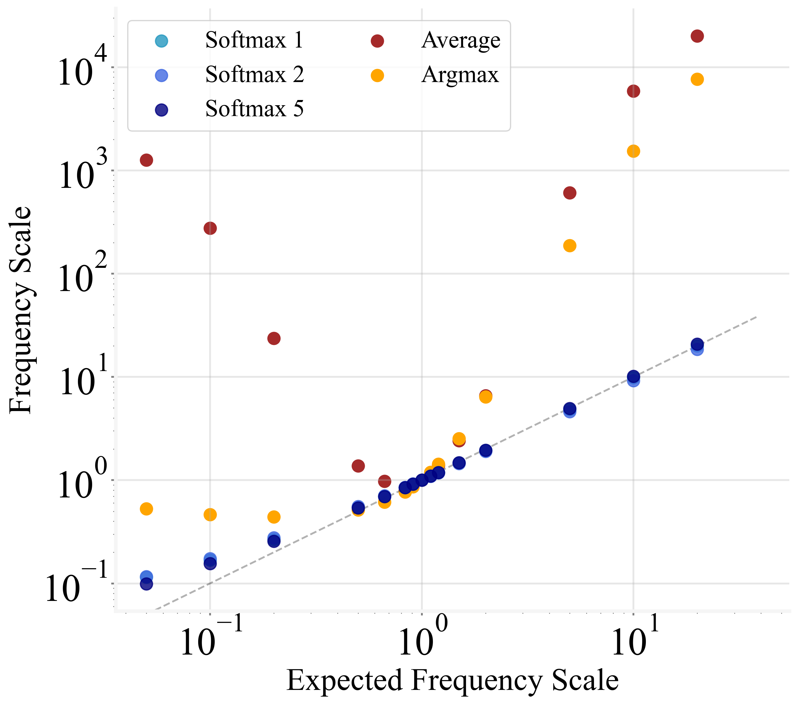
Figure 8: The expected probability scales and the actually edited scales measured in the edited LMs w.r.t. different values of $b$.

(a) GPT2-XL, 1.6B

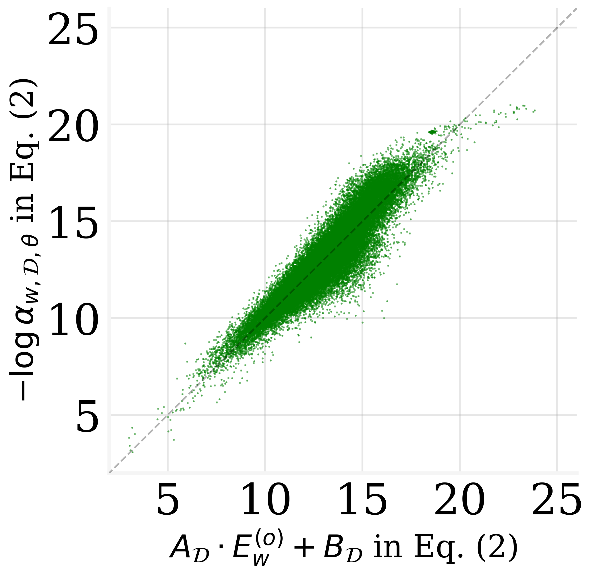
(b) Pythia, 2.8B

Figure 9: Supplement for Fig. 2. The MLR results on GPT2-XL and Pythia-2.8B.

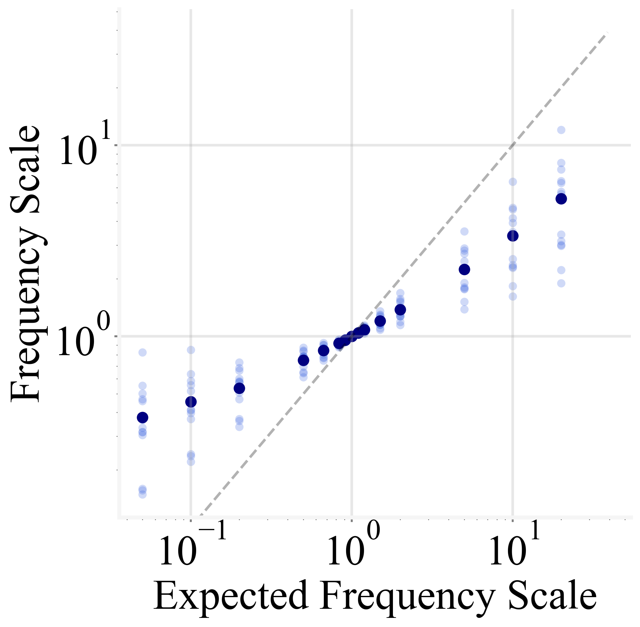
Figure 10: Supplement for Fig. 4. The expected probability scales and the actually edited scales measured in the edited GPT2-XL.

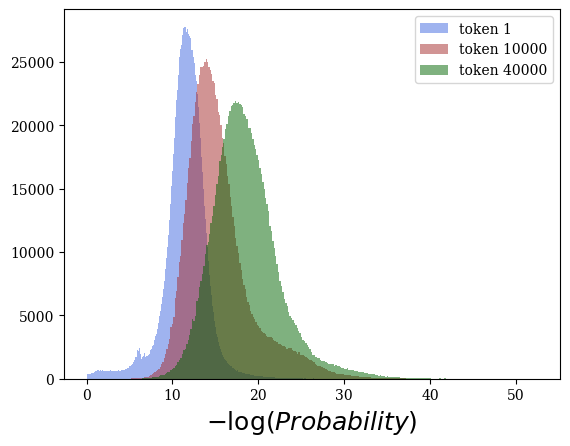
(a) GPT2, 137M

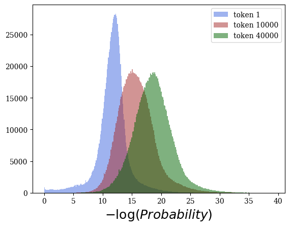
(b) GPT2-XL, 1.6B

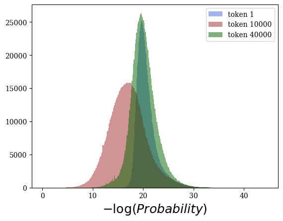
(c) Pythia, 2.8B

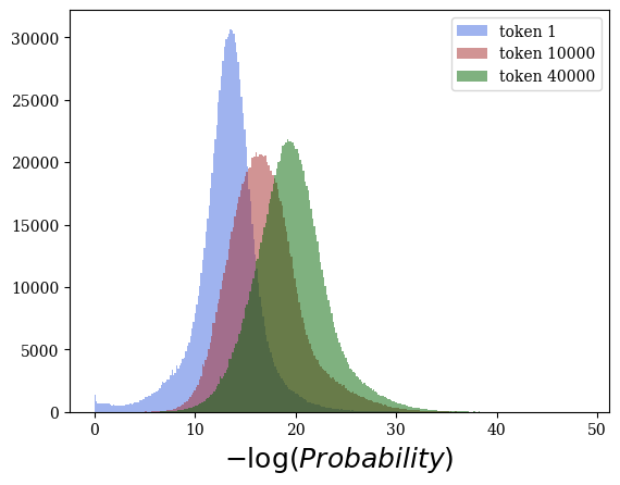
(d) GPT-J, 6B

Figure 11: Examples of the probability distribution of one token among input prefixes.

As mentioned before, Kobayashi et al. (2023) mainly found a correlation between the output token probability and the bias term in the LM head and tried to remove this bias towards more diversified text generation. However, they didn’t analyze the output embedding matrix, which has the most parameters in the LM head, and this paper completes their research.

Geometry of Input Embedding.

As a similar research object with the output embedding, it was found that the word embeddings in LMs, as well as the hidden states, are anisotropy Mu and Viswanath (2018); Ethayarajh (2019); Gao et al. (2018), i.e., these vectors share a common bias and a close direction. Such anisotropies hurt the expressiveness of word embeddings, and the word frequency in the corpus may be an inducement Mu and Viswanath (2018); Valentini et al. (2023). Also, some efforts tried to remove the harmfulness of anisotropies and towards isotropy word embeddings Mu and Viswanath (2018); Gong et al. (2018). These works are based on input embedding, while our paper is on output embedding. Although we can confirm that the input and output embeddings act similarly, they are still completely different components of untied LMs. So the existing conclusions on input embeddings cannot overwrite our work.

Embedding Tying in LMs.

LMs in previous generations often have a shared output embedding from the input embedding, such as BERT Kenton and Toutanova (2019), RoBERTa Liu et al. (2019), GPT2 Radford et al. (2019), etc. That is, the LM head maps the last hidden state to the token probability by dpt-producing the input embedding. Such a paradigm is recommended by Press and Wolf (2017) for fewer parameters. And also refuted by Chung et al. (2020) for a harmfulness to expressiveness. Such a paradigm is being deprecated currently, but the model behavior with and without embedding tying is still interesting to analyze.

(Language) Model Editing and Model Pruning.

Recent Large LMs are expensive to fine-tune or retrain, so there are many model editing methods to control the output of LMs Yao et al. (2023). Current LM parameter editing methods are mainly oriented to entity relationship editing, where they locate some parameters with correlations to the entities, and interference is applied on such parameters Dai et al. (2022); Meng et al. (2022). Moreover, vectorized methods are also proposed with the arithmetic of parameter vectors with editing information Ilharco et al. (2022); Ortiz-Jimenez et al. (2024). As a specific and extreme scenario of model editing, research on model pruning, similar to our dimension removing is also proposed in current years Zhu et al. (2023); Frantar and Alistarh (2023); Kovaleva et al. (2021); Timkey and van Schijndel (2021); Gordon et al. (2020). These pruning are usually unsupervised, where our dimension removing can be a new practice in the supervised pruning paradigm.

Training Dynamics (of LMs).

Investigating what is happening in the training process of language models and other deep learning models is an attractive research topic. Many works about training trajectory Kalra and Barkeshli (2024); Jastrzębski et al. (2018); Lewkowycz et al. (2020), early period training behaviors Frankle et al. (2019); Kalra and Barkeshli (2024); Achille et al. (2018), loss landscape Neyshabur et al. (2020); Keskar et al. (2017); Li et al. (2018), and "knowledge" earned in different stages of training Tirumala et al. (2022); Liu et al. (2021) have been done. Differences in training speed among various network layers (the deeper-slower pattern) have been discovered by Chen et al. (2022), while in this paper, following their method, we don’t find a similar pattern.

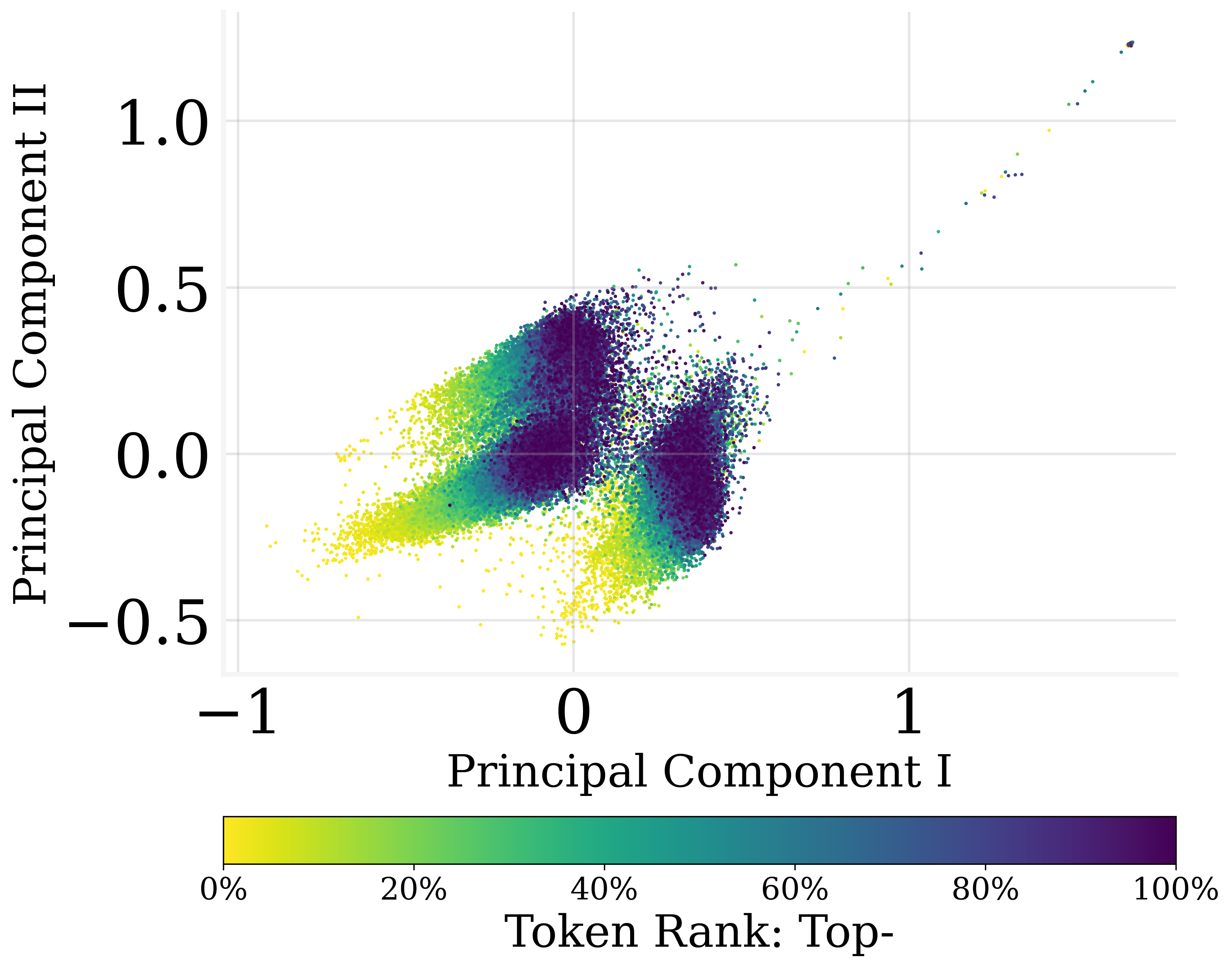
(a) GPT2-XL, 1.6B

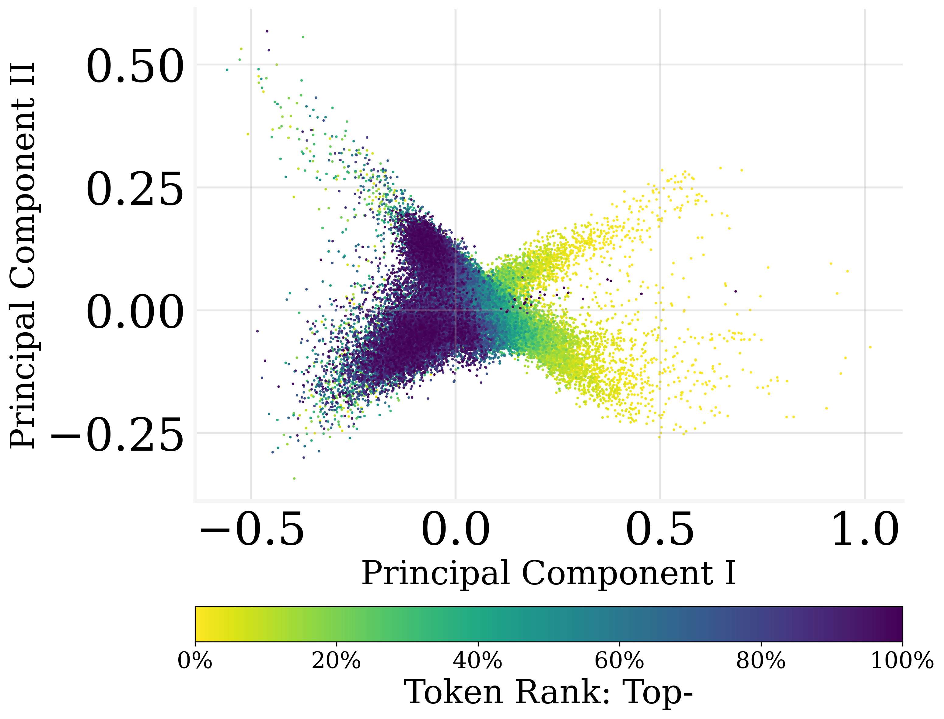
(b) Pythia, 2.8B

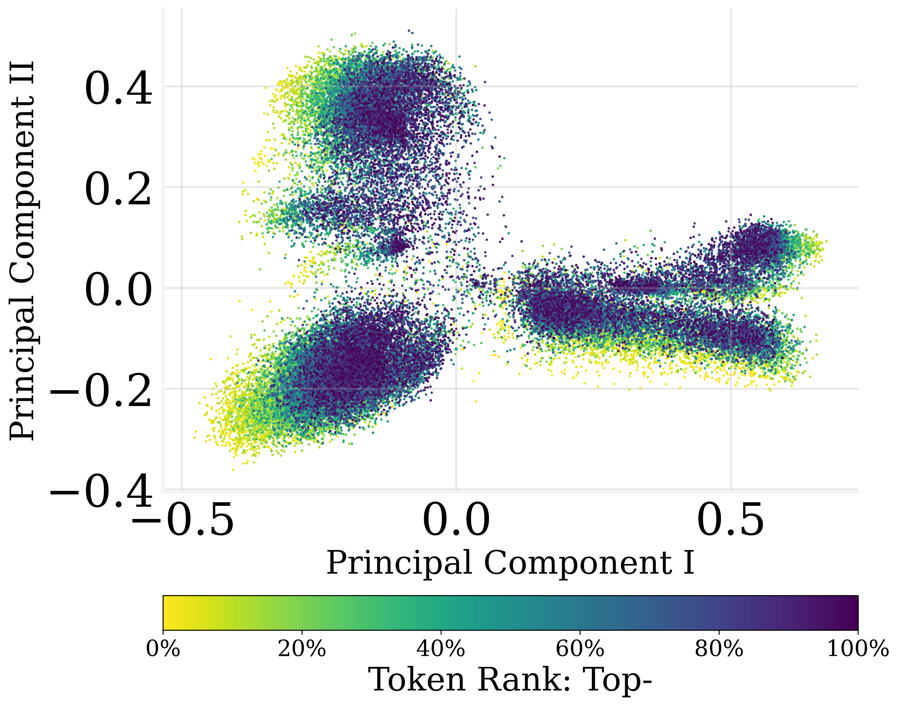
(c) GPT-J, 6B

Figure 12: Supplement for Fig. 1. Output embedding visualizations w.r.t. output token probability for GPT2-XL, Pythia, GPT-J.

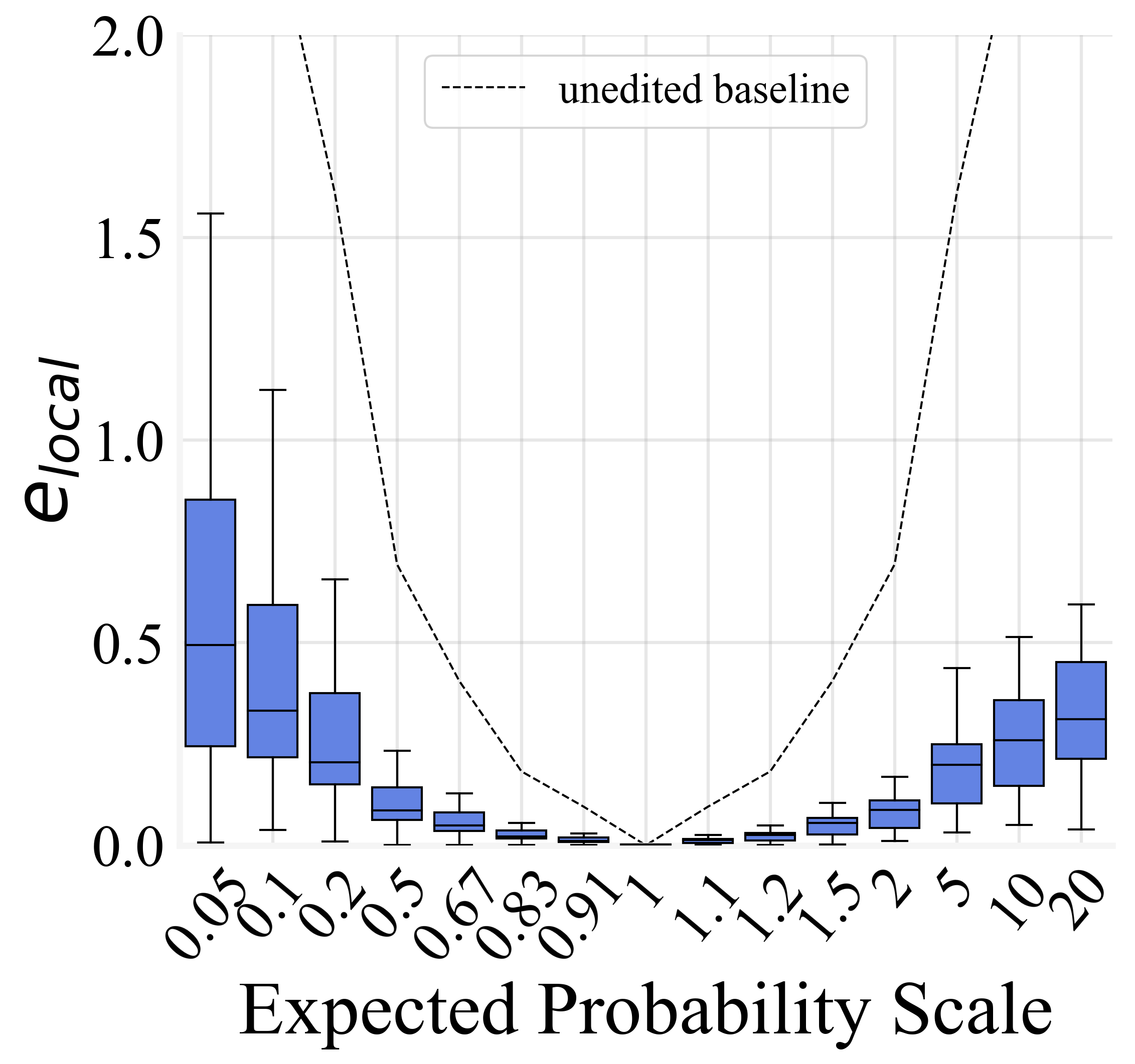
(a) $e_{local}$

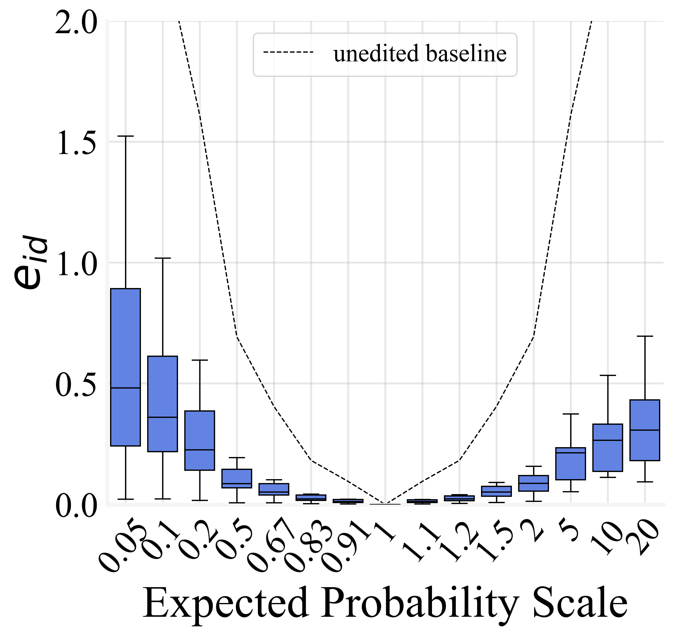
(b) $e_{id}$

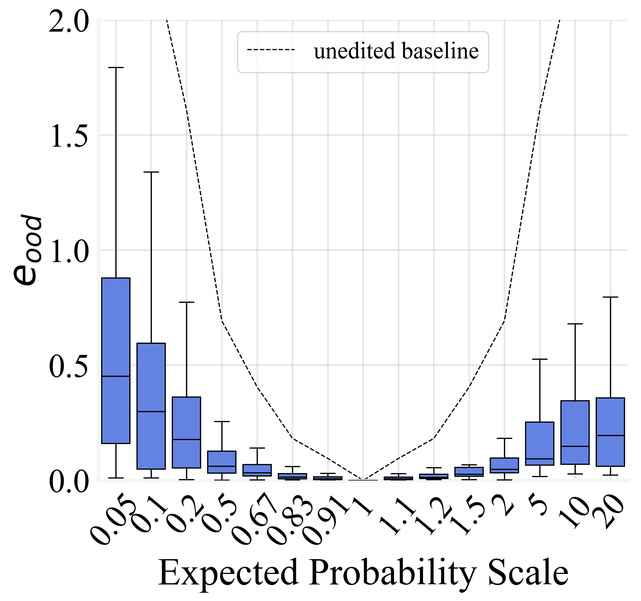
(c) $e_{ood}$

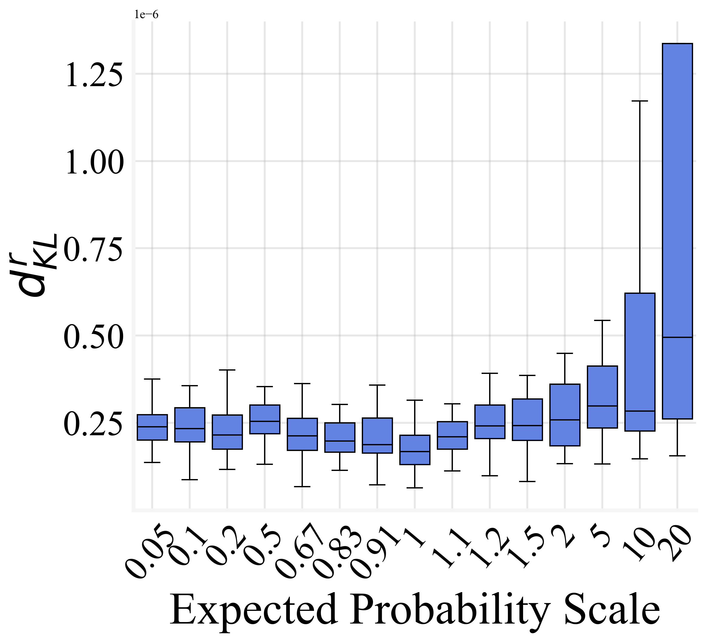
(d) $d_{KL}^{r}$

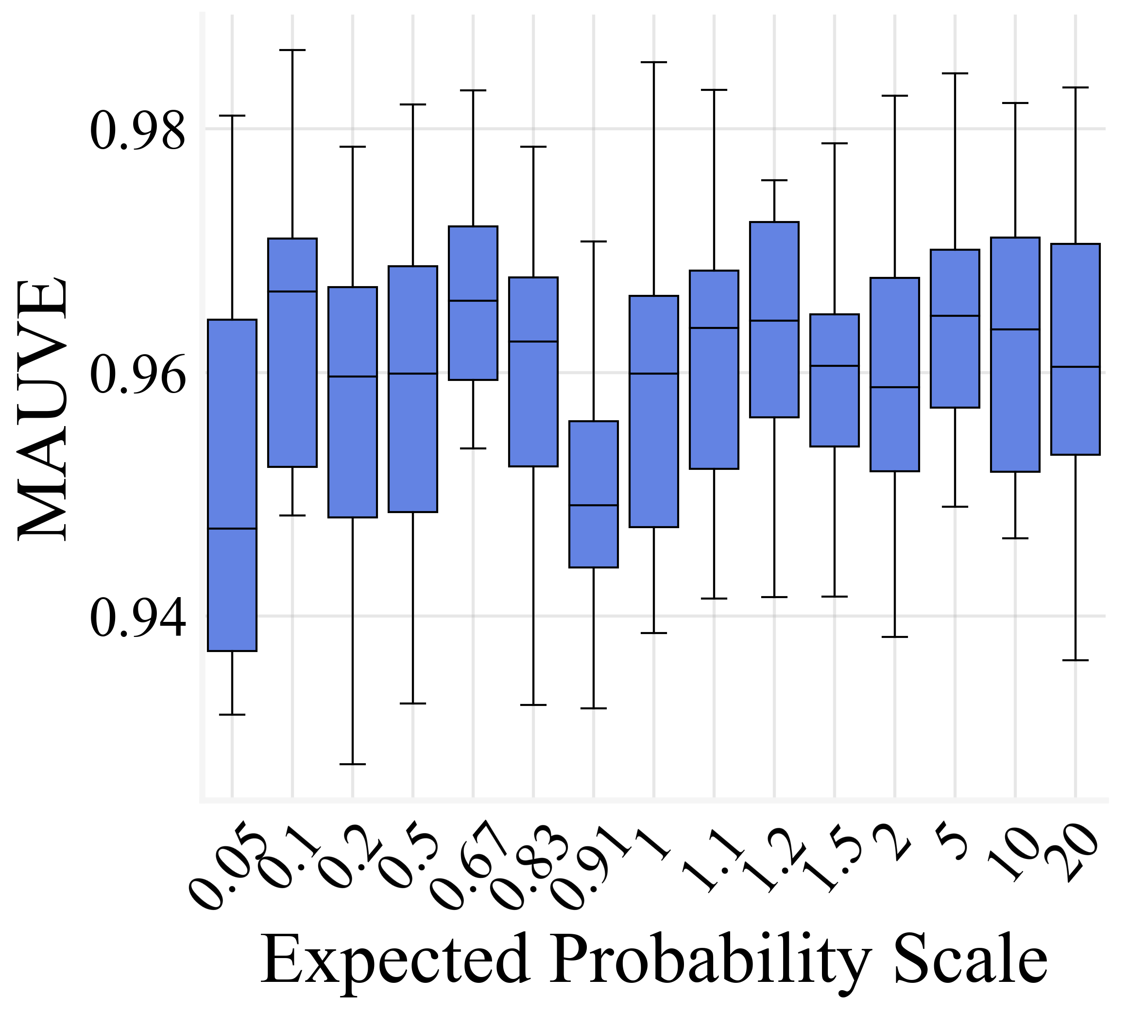
(e) $MAUVE$

Figure 13: Fine-grained results w.r.t. expected editing scales of GPT2.

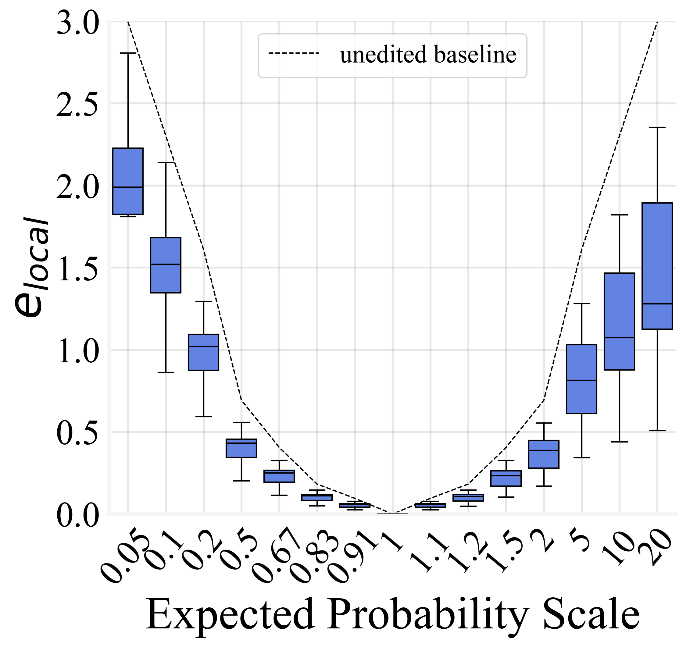
(a) $e_{local}$

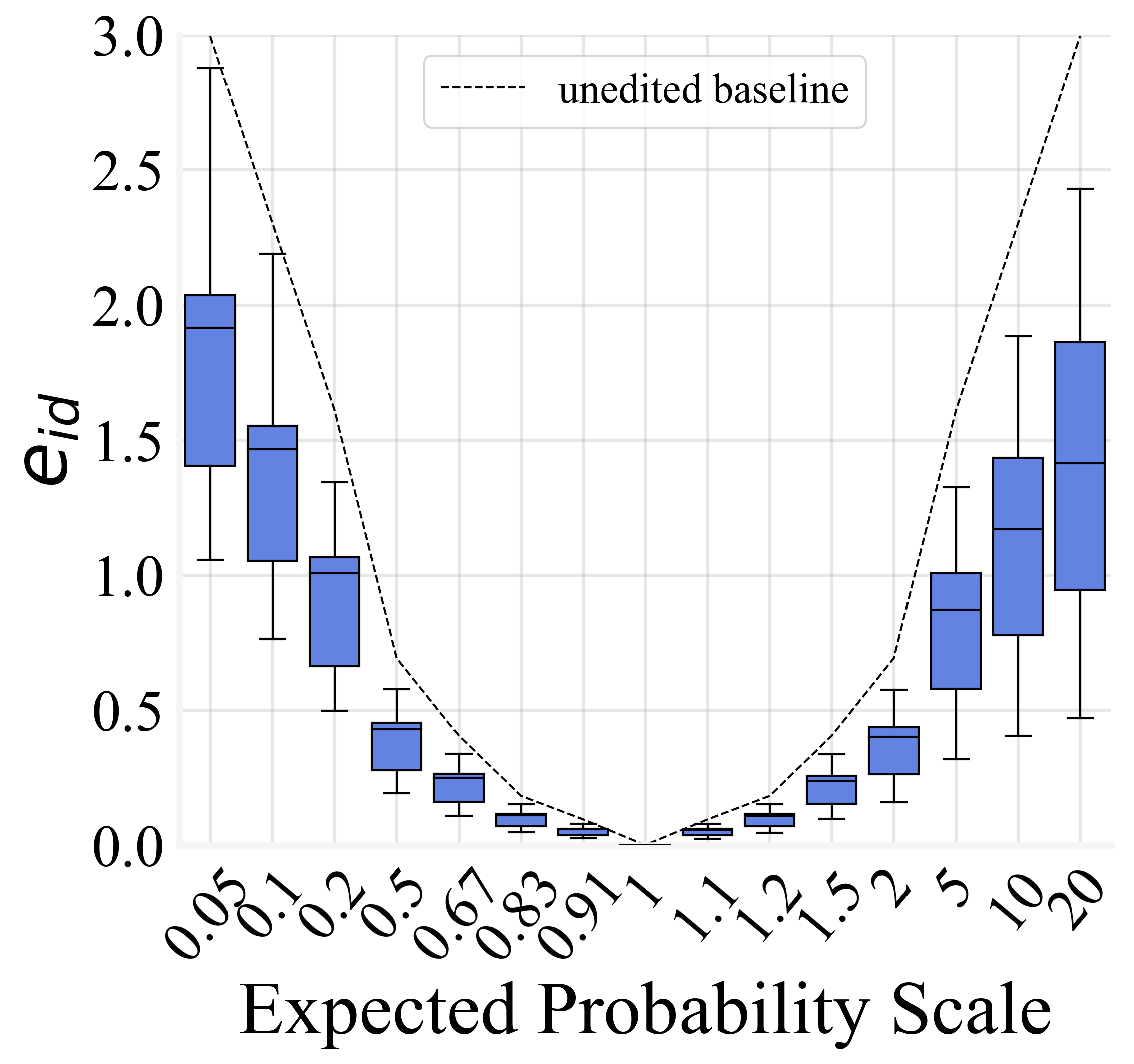
(b) $e_{id}$

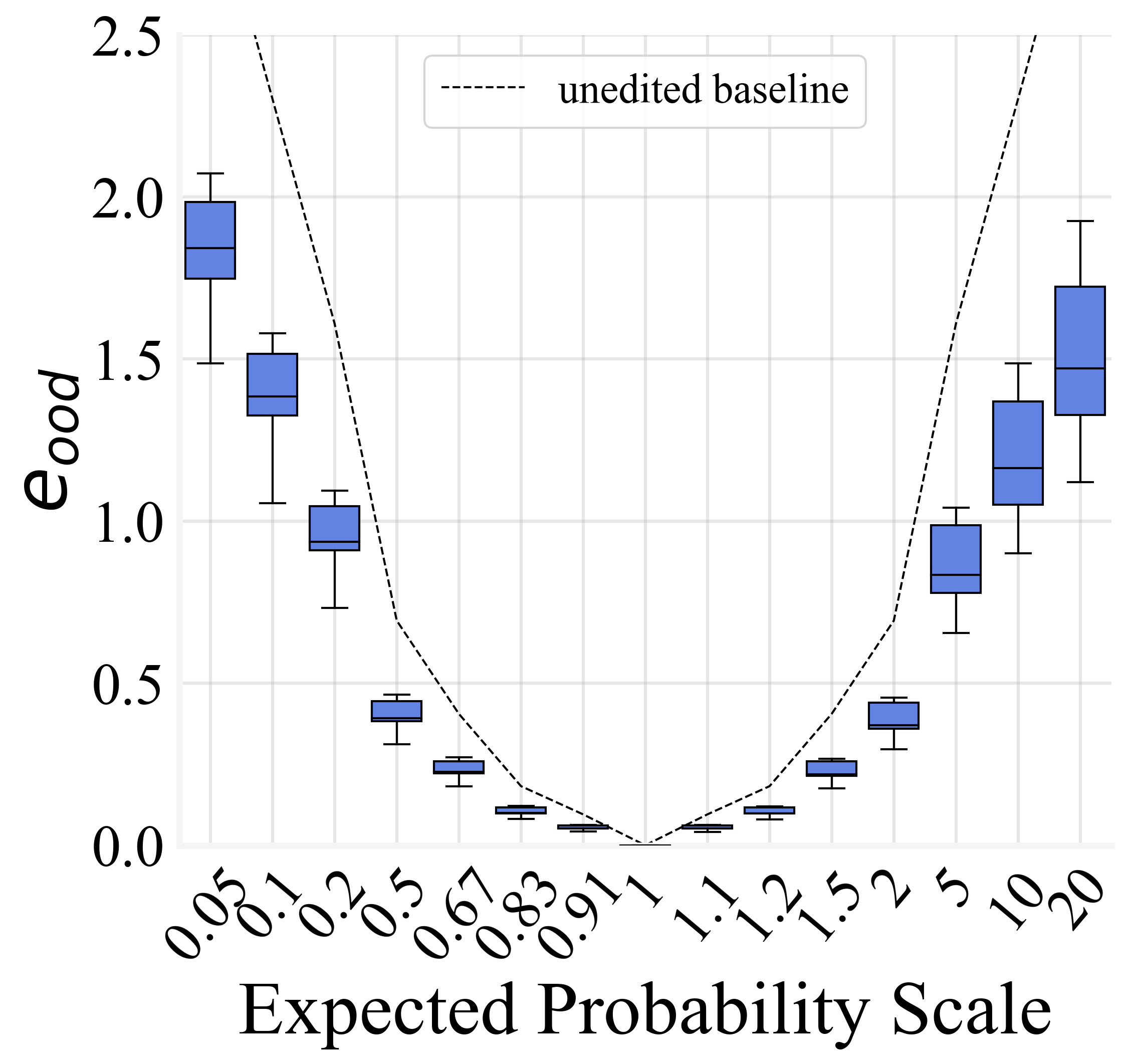
(c) $e_{ood}$

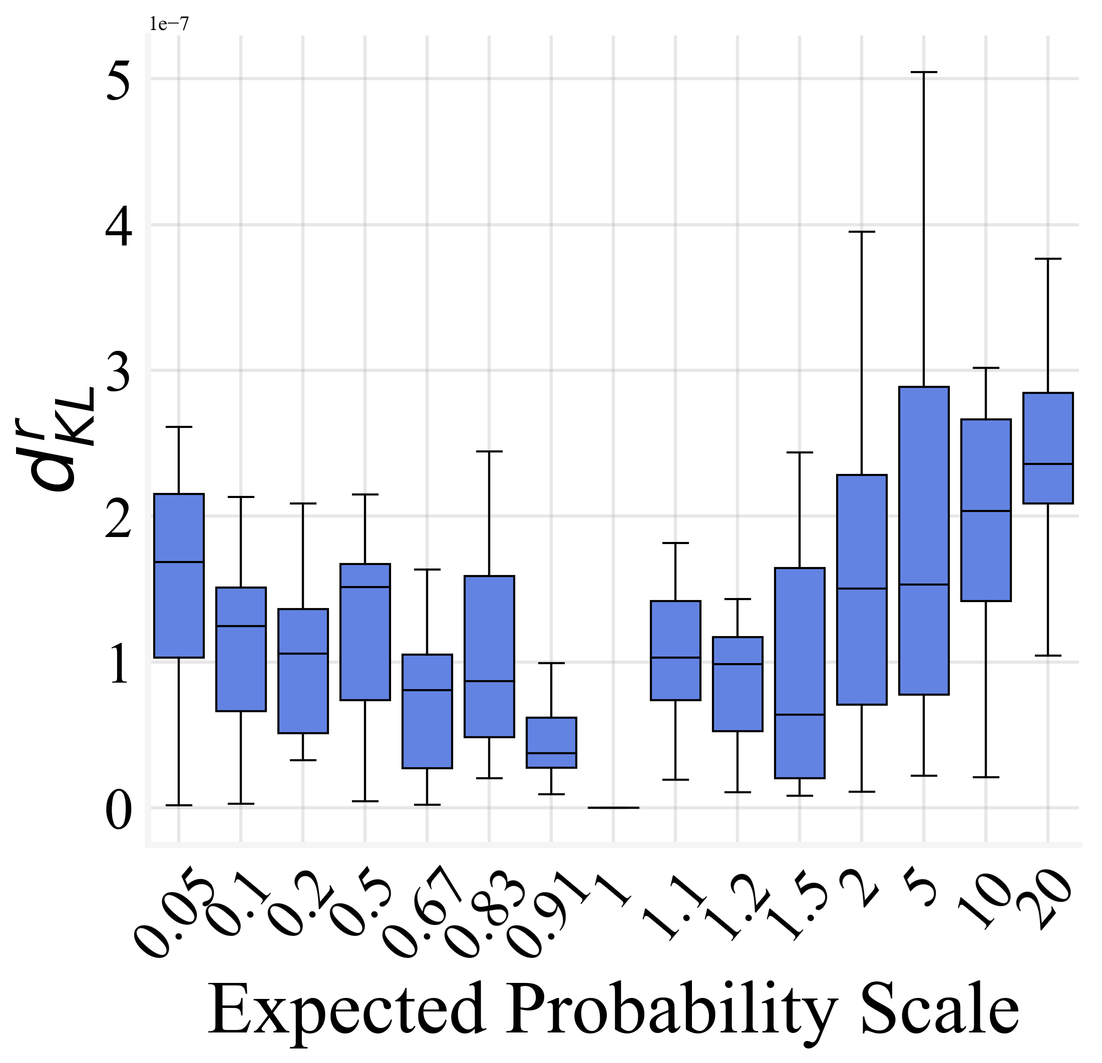
(d) $d_{KL}^{r}$

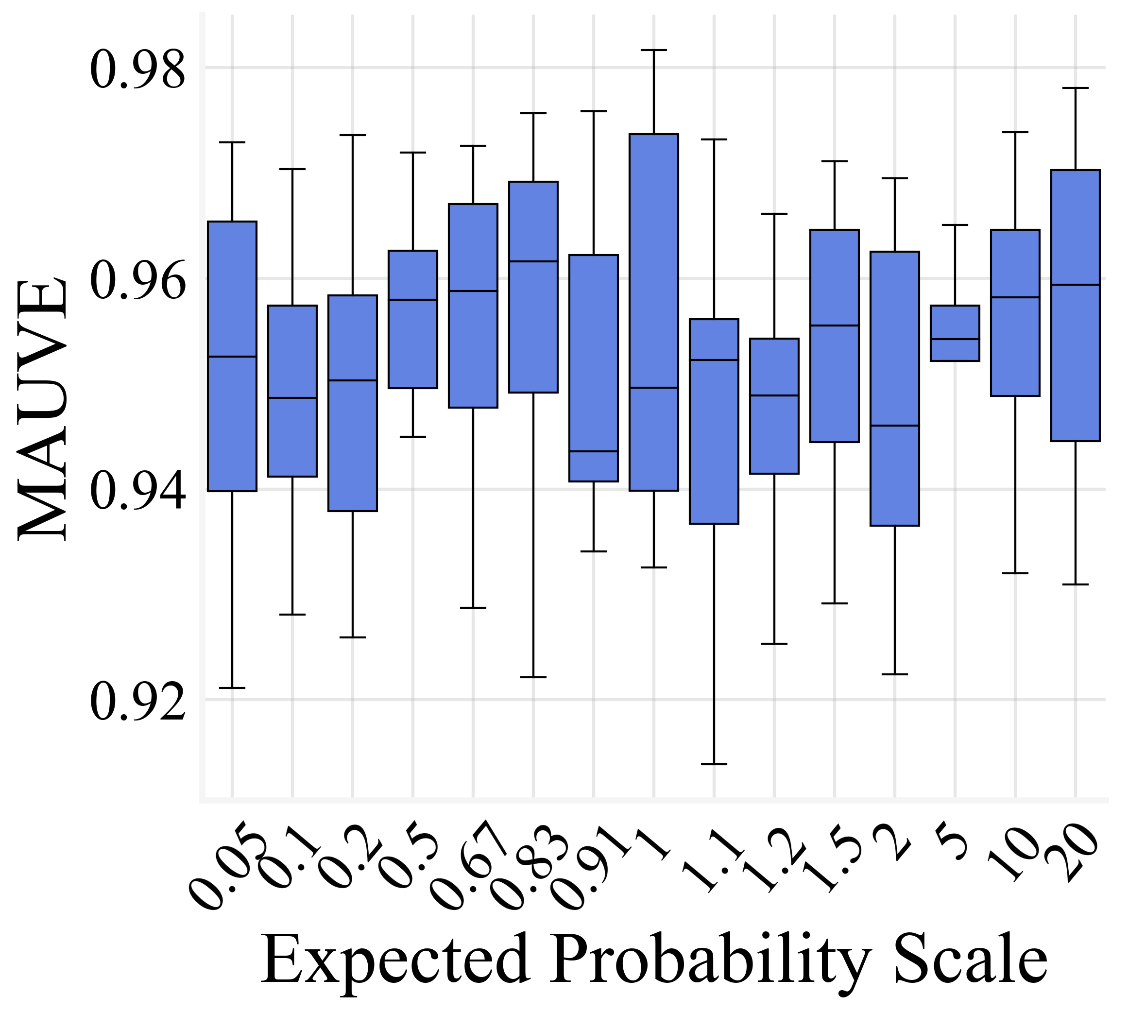
(e) $MAUVE$

Figure 14: Fine-grained results w.r.t. expected editing scales of GPT2-XL.

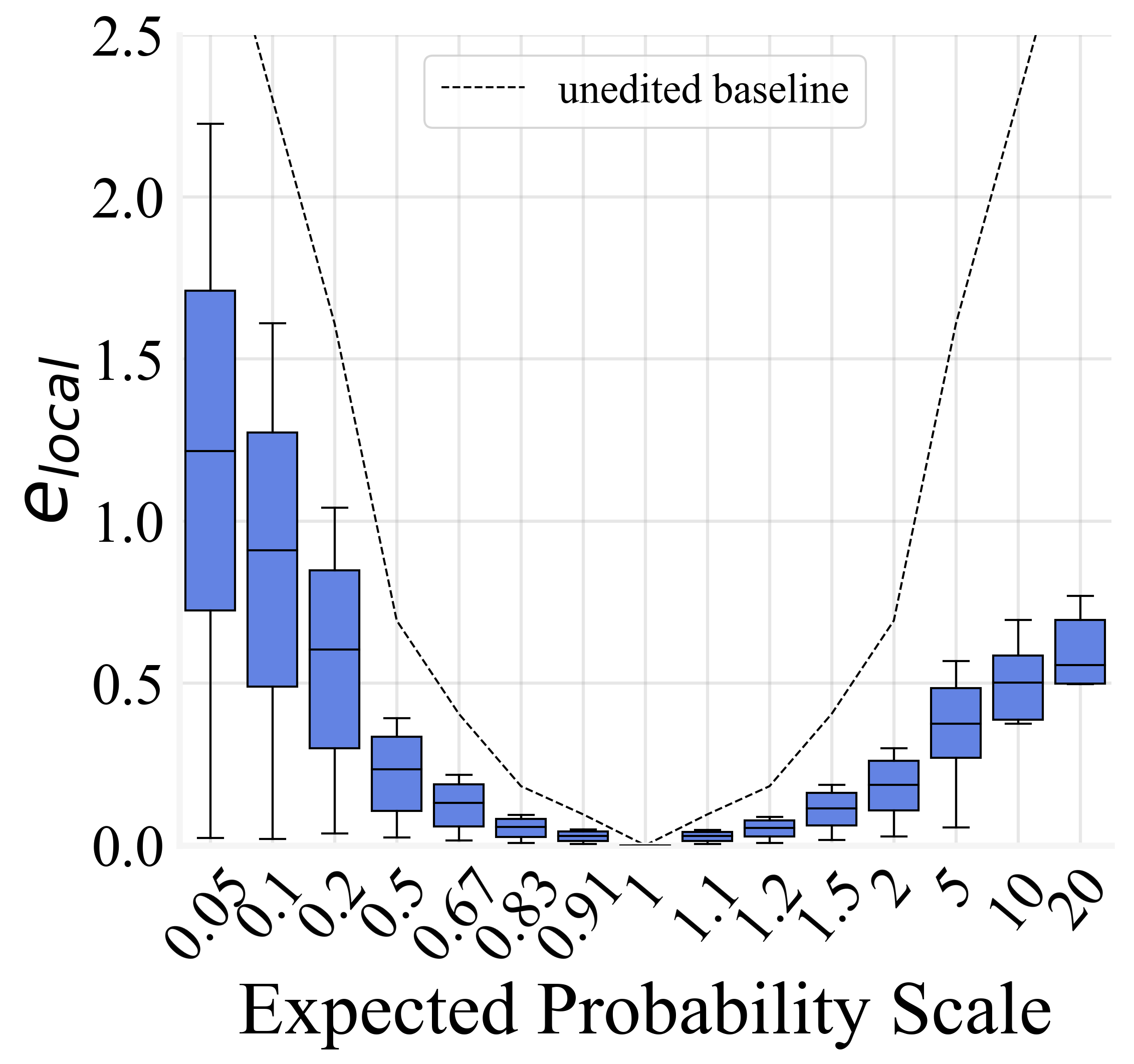
(a) $e_{local}$

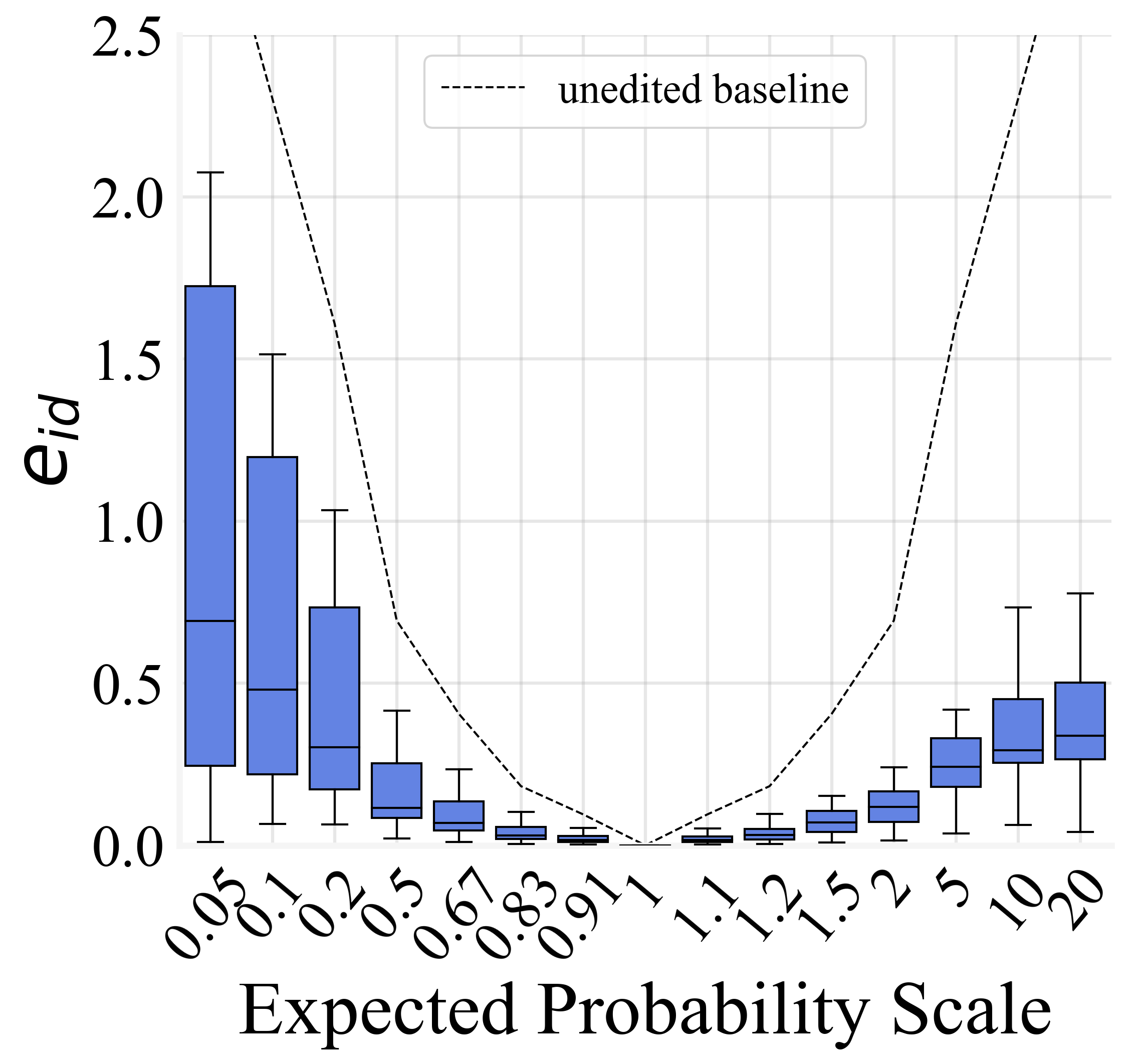
(b) $e_{id}$

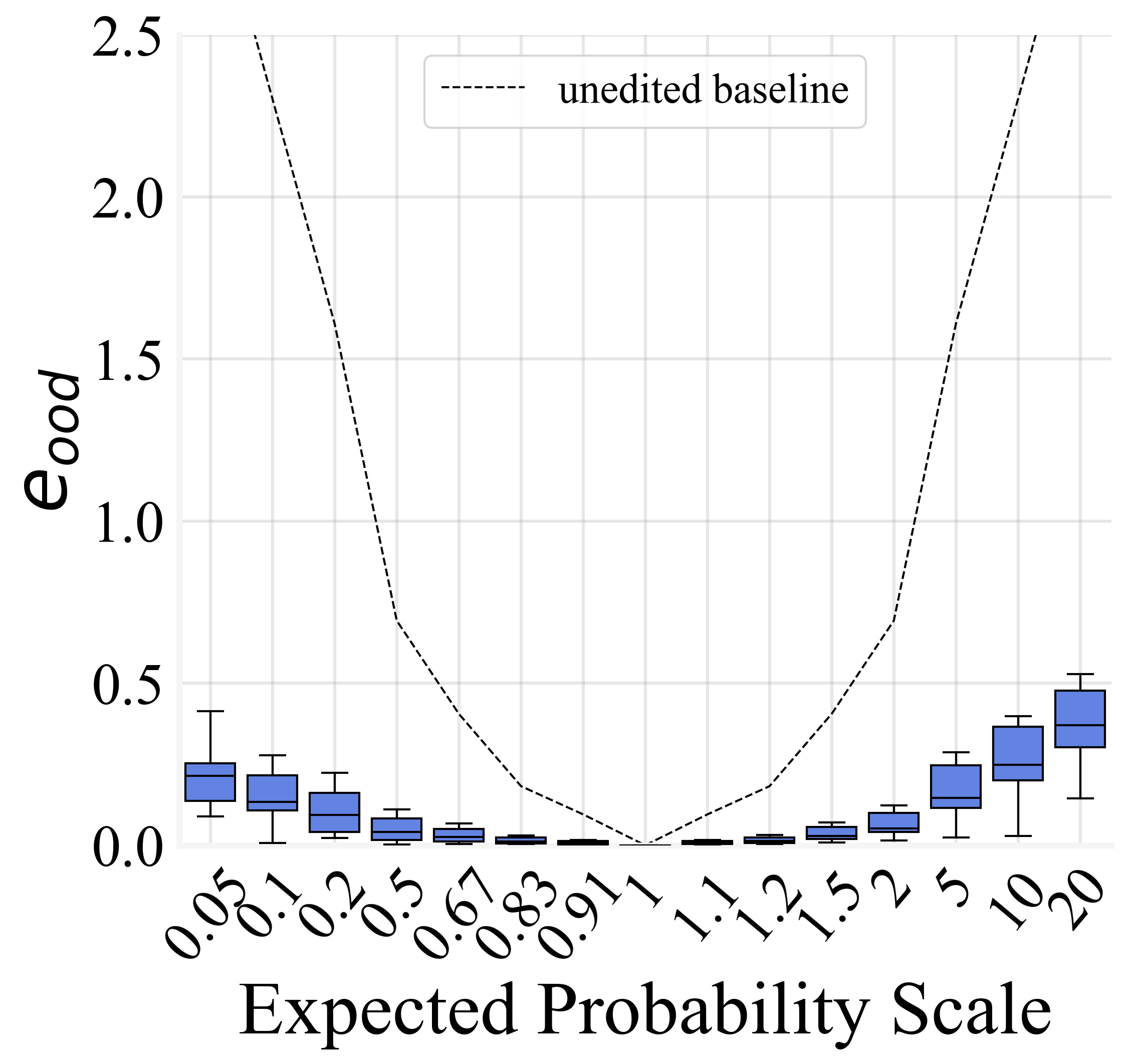
(c) $e_{ood}$

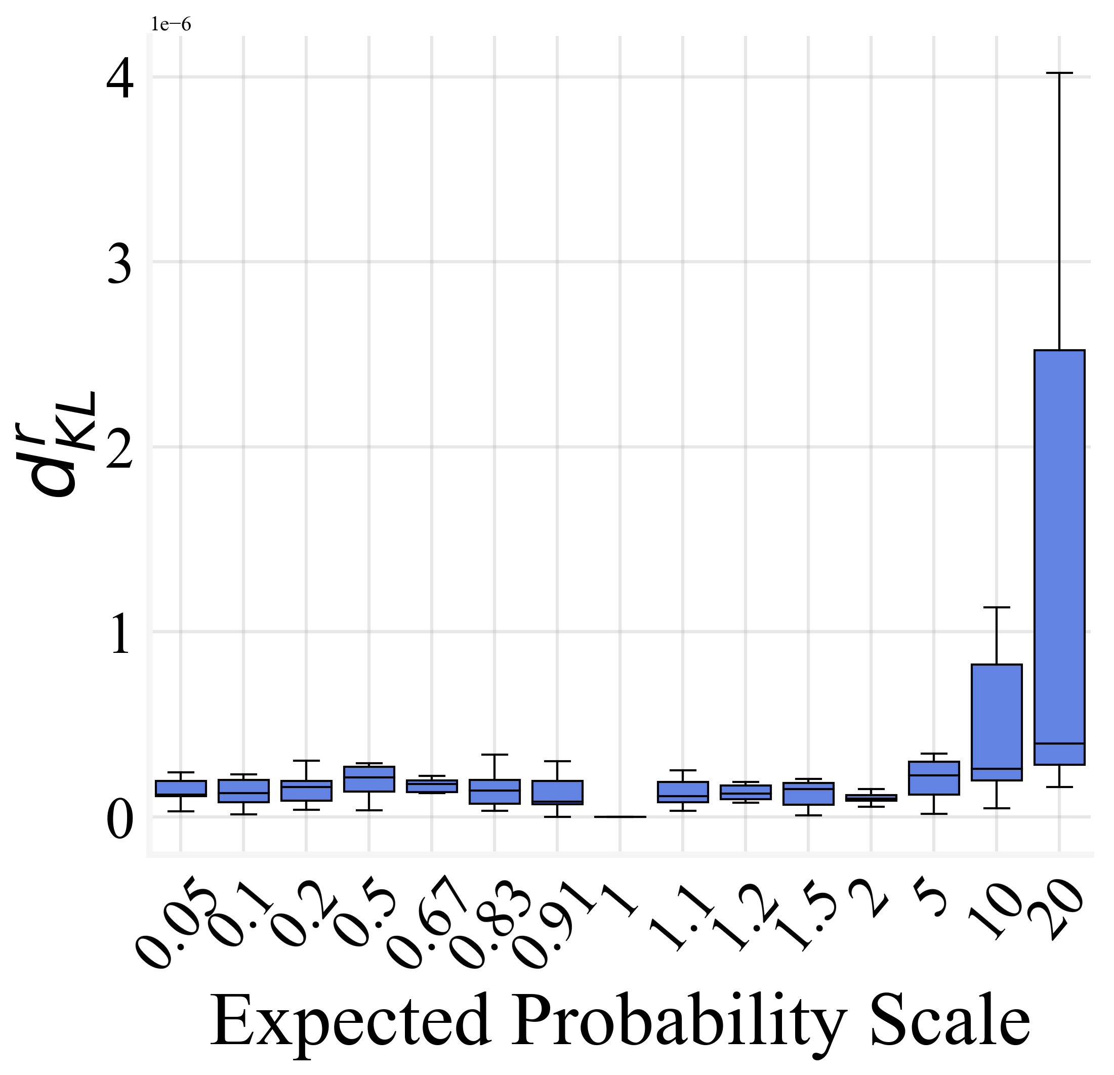
(d) $d_{KL}^{r}$

Figure 15: Fine-grained results w.r.t. expected editing scales of GPT-J.

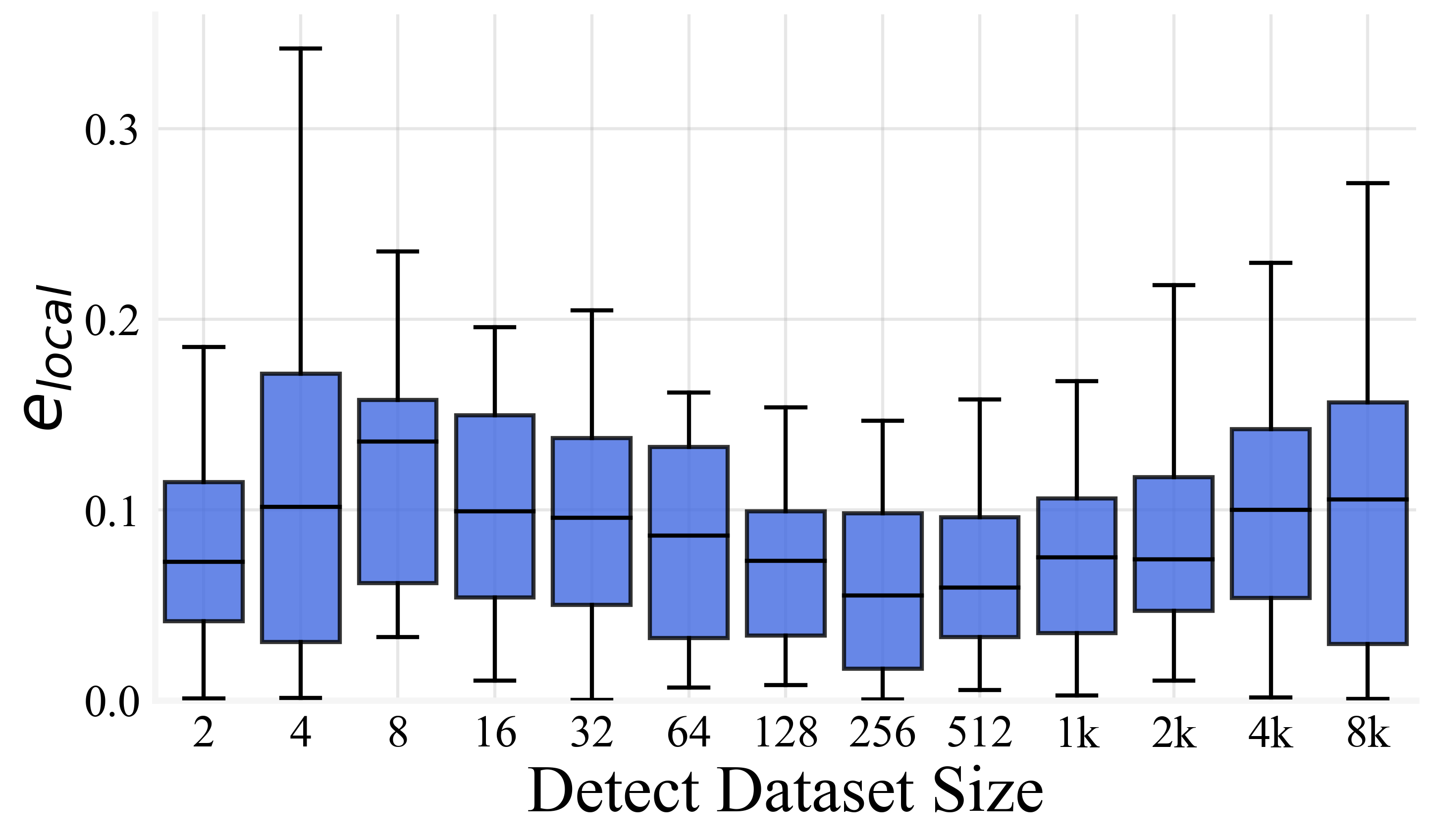
(a) $e_{local}$

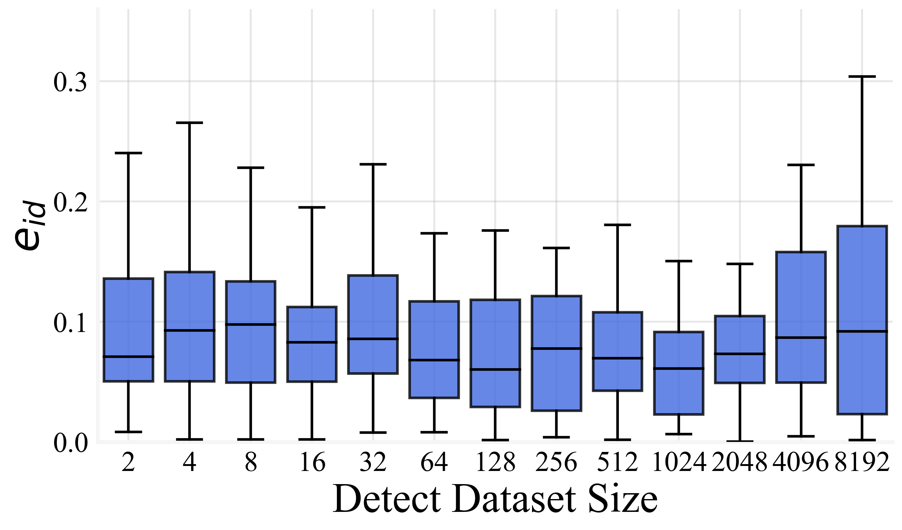
(b) $e_{id}$

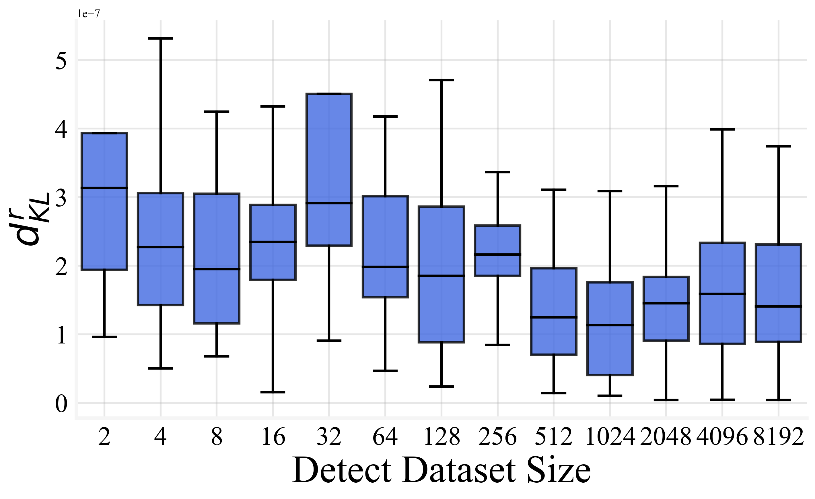
(c) $d_{KL}^{r}$

Figure 16: Supplement for Fig. 5. The $e_{local}$, $e_{id}$, $d_{KL}^{r}$ w.r.t. the detect dataset size.

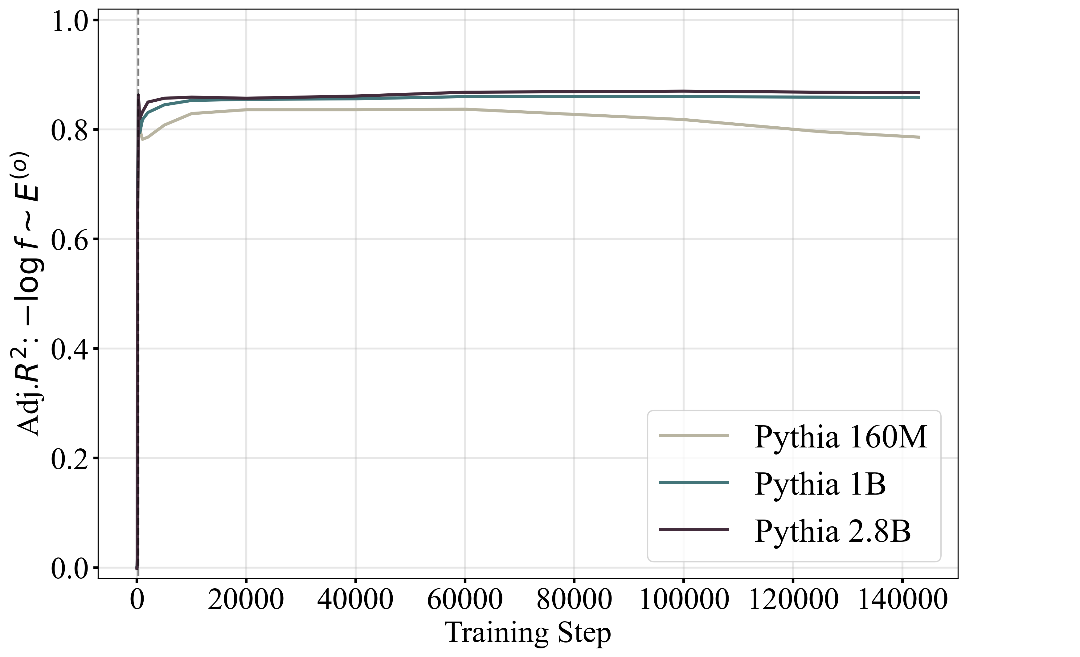
(a)

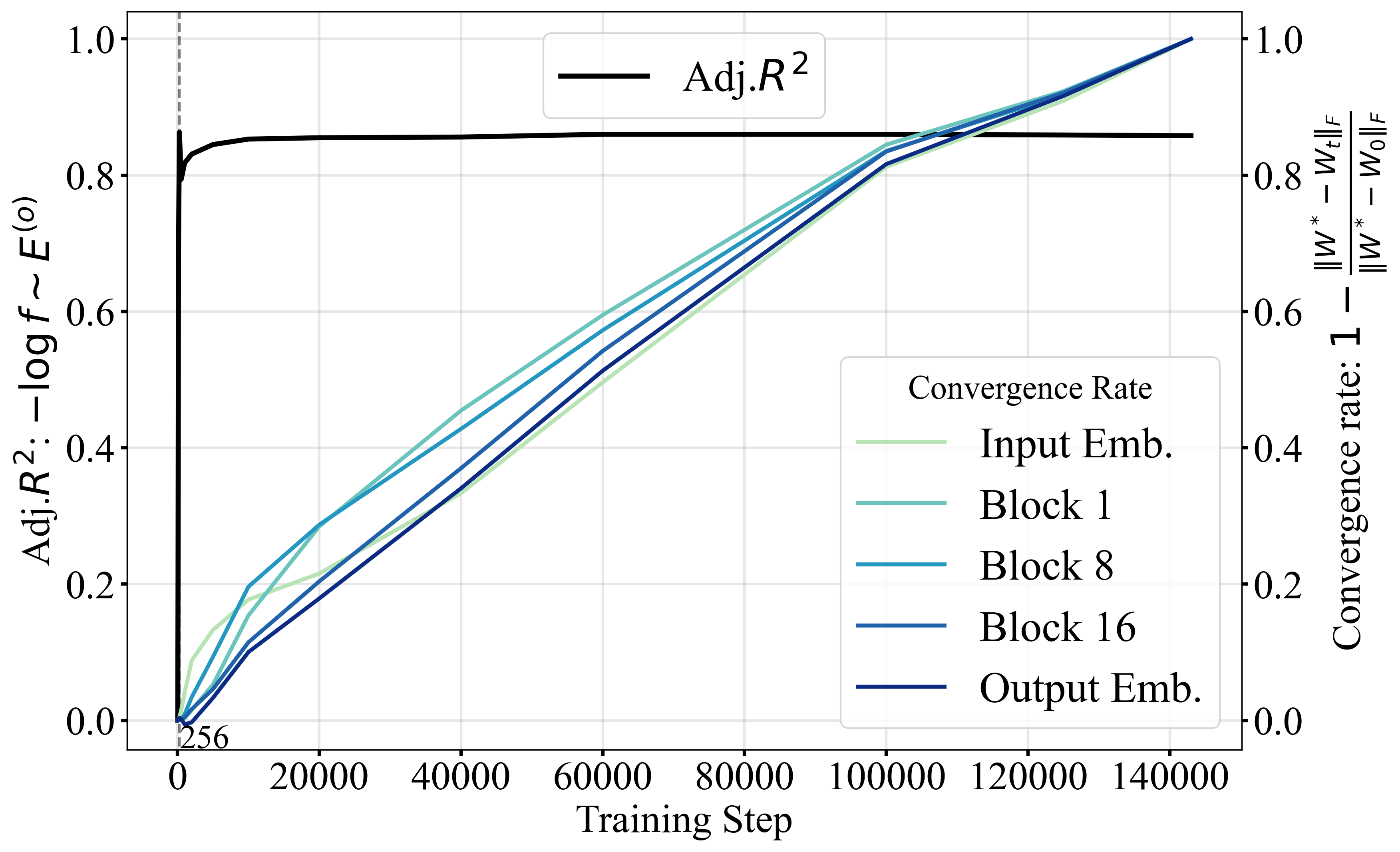
(b)

Figure 17: Supplement for Fig. 7. Without log-scaling.

Appendix B Calculation Details

B.1 Calculation of Averaged Token Probability

Given a dataset $\mathcal{D}=\{x_{i}\}_{i=1}^{m}$, we input each $x_{i}$ into LMs in a teacher forcing style. Denote the length of $x_{i}$ as $l_{i}$, we can get output token probability distribution on each time step (noted as $j$) $\alpha_{\mathcal{D},\theta,i,j}\in\mathbb{R}^{|\mathbb{V}|}$ of an amount of $l_{i}$.

We average all the $\alpha_{\mathcal{D},\theta,i,j}$ on every $i$ and $j$, and get the averaged token probability distribution $\alpha_{\mathcal{D},\theta}$ on dataset $\mathcal{D}$.

B.2 Error Analysis of Eq. 1

In Eq. 1, we do a local linear approximation as:

$$\begin{split}-\log\alpha_{w,\mathcal{D},\theta}&=-\log\mathbb{E}_{x\in\mathcal{D}}[P_{\theta}(w|x)]\\ &\approx\mathbb{E}_{x\in\mathcal{D}}[-\log[P_{\theta}(w|x)]].\\ \end{split}$$

That is, given a set of $\{p_{i}\}_{i=0}^{n}$, where $\forall i,p_{i}>0$ we approximate that $\log\mathbb{E}_{i\in[0,n]}[p_{i}]\approx\mathbb{E}_{i\in[0,n]}[\log p_{i}]$. Assume that we have a non-descending sequence of $p$, that is, $p_{0}\leq p_{1}\leq p_{2}\leq\dots\leq p_{n}$, w.l.o.g. We can confirm that $\mathbb{E}_{i\in[0,n]}[p_{i}]\in[p_{0},p_{n}]$. So we have: $\exists\xi\in(p_{0},\mathbb{E}_{i\in[0,n]}[p_{i}]),s.t.$,

$$\log\mathbb{E}_{i\in[0,n]}[p_{i}]=\frac{1}{\xi}(\mathbb{E}_{i\in[0,n]}[p_{i}]-p_{0})+\log p_{0}$$

We have:

$$\mathbb{E}_{i\in[0,n]}[\log p_{i}]\geq\log p_{0},$$

since $\log^{\prime}(\cdot)>0$. That is:

$$\begin{split}&[\log\mathbb{E}_{i\in[0,n]}[p_{i}]-\mathbb{E}_{i\in[0,n]}[\log p_{i}]]^{2}\\ \leq&\frac{1}{\xi^{2}}(\mathbb{E}_{i\in[0,n]}[p_{i}]-p_{0})^{2}\\ \leq&\frac{1}{p_{0}^{2}}(\mathbb{E}_{i\in[0,n]}[p_{i}]-p_{0})^{2}.\end{split}$$ (3)

We can empirically confirm the concentration of $p_{i}$, shown as examples in Fig. 11, which makes the error shown in Eq. 3 acceptably small. Additionally, a low-probability token shows a wide probability distribution, which is consistent with our findings in Fig. 2, where a low-probability token is assigned with more inaccurate predictions (manifested as a comet-shaped figure).

B.3 Details of MAUVE Calculation

The MAUVE is a similarity between two datasets. Refer Pillutla et al. (2021) for the calculating details of MAUVE. Here we explain our method to get both datasets for MAUVE to measure the harmfulness of our model editing method. We sample 512 data points from the BookCorpus Zhu et al. (2015), and take the first two words of each data point as a prefix to collect a prefix set. Given a generative language model, we input the prefixes and let the model generate naturally into a generated dataset. We do this process on the original model and the edited model and use the two generated datasets to calculate the MAUVE.

Appendix C Ablation Study on Editing Amount Allocation Parameter $b$

We discuss the editing amount allocation parameter $b$ in Algorithm 1. We try different settings of $b$ on GPT2 as shown in Table 3 and Fig. 8.

The results show that when the $b$ is not infinities, the editing remains accurate and stable. That is, the algorithm is not sensitive to a positive integer $b$. But we still recommend a large $b$ when the model is large and the sparsity of MLR slope is not fine.

However, when the $b$ is $+\infty$ or $-\infty$, the editing can not be accurate and is easy to get a larger scale than expected. We infer that both of these infinity $b$ increase the norm of the embedding vector too much, leading to an increase in its output probability as well.

Appendix D Supplementary Experiment Results

Supplement for Fig. 1. Output embedding visualizations w.r.t. output token probability for GPT2-XL, Pythia, GPT-J are shown in Fig. 12.

Supplement for Fig. 2. Output probability fitting results of GPT2-XL and Pythia-2.8B are shown in Fig. 9.

Supplement for Fig. 4. The expected probability scales and the actually edited scales of GPT2-XL is shown in Fig. 10.

Supplement for Table 2. Fine-grained results w.r.t. expected editing scales of GPT2 (Fig. 13), GPT2-XL (Fig. 14), GPT-J (Fig. 15).

Supplement for Fig. 5. The $e_{local}$, $e_{id}$, $d_{KL}^{r}$ w.r.t. the detect dataset size are shown in Fig. 16.

Supplement for Fig. 7. The figures without log-scaling are shown in Fig. 17.

Appendix E Necessary Statements

Repeatability statement.

Models and datasets are all loaded from huggingface. All the datasets are shuffled with random seed 42 and cut into required slices. We calculate MAUVE by the package mauve-text by default parameters. In experiments, all the logarithms are natural.

License of the artifacts.

The artifacts used in this paper are all open-sourced and are used for their intended usage.

Models. GPT2 family are under the MIT license, GPT-J and Pythia are under the apache-2.0 license.

Datasets. WikiDpr is under the cc-by-nc-4.0 license, BookCorpus and Pile is under the MIT license.

Tool. MAUVE is under the GNU license.

References

- Achille et al. (2018) Alessandro Achille, Matteo Rovere, and Stefano Soatto. 2018. Critical learning periods in deep networks. In International Conference on Learning Representations.
- Ba et al. (2016) Jimmy Lei Ba, Jamie Ryan Kiros, and Geoffrey E Hinton. 2016. Layer normalization. arXiv preprint arXiv:1607.06450.
- Biderman et al. (2022) Stella Biderman, Kieran Bicheno, and Leo Gao. 2022. Datasheet for the pile. arXiv preprint arXiv:2201.07311.
- Biderman et al. (2023) Stella Biderman, Hailey Schoelkopf, Quentin Gregory Anthony, Herbie Bradley, Kyle O’Brien, Eric Hallahan, Mohammad Aflah Khan, Shivanshu Purohit, USVSN Sai Prashanth, Edward Raff, et al. 2023. Pythia: A suite for analyzing large language models across training and scaling. In International Conference on Machine Learning, pages 2397–2430. PMLR.
- Chen et al. (2022) Yixiong Chen, Alan Yuille, and Zongwei Zhou. 2022. Which layer is learning faster? a systematic exploration of layer-wise convergence rate for deep neural networks. In The Eleventh International Conference on Learning Representations.
- Chung et al. (2020) Hyung Won Chung, Thibault Fevry, Henry Tsai, Melvin Johnson, and Sebastian Ruder. 2020. Rethinking embedding coupling in pre-trained language models. In International Conference on Learning Representations.
- Dabkowski and Gal (2017) Piotr Dabkowski and Yarin Gal. 2017. Real time image saliency for black box classifiers. Advances in neural information processing systems, 30.
- Dai et al. (2022) Damai Dai, Li Dong, Yaru Hao, Zhifang Sui, Baobao Chang, and Furu Wei. 2022. Knowledge neurons in pretrained transformers. In Proceedings of the 60th Annual Meeting of the Association for Computational Linguistics (Volume 1: Long Papers), pages 8493–8502.
- Ethayarajh (2019) Kawin Ethayarajh. 2019. How contextual are contextualized word representations? comparing the geometry of bert, elmo, and gpt-2 embeddings. In Proceedings of the 2019 Conference on Empirical Methods in Natural Language Processing and the 9th International Joint Conference on Natural Language Processing (EMNLP-IJCNLP), pages 55–65.
- Fei et al. (2023) Yu Fei, Yifan Hou, Zeming Chen, and Antoine Bosselut. 2023. Mitigating label biases for in-context learning. In The 61st Annual Meeting Of The Association For Computational Linguistics.
- Frankle et al. (2019) Jonathan Frankle, David J Schwab, and Ari S Morcos. 2019. The early phase of neural network training. In International Conference on Learning Representations.
- Frantar and Alistarh (2023) Elias Frantar and Dan Alistarh. 2023. Sparsegpt: Massive language models can be accurately pruned in one-shot. In International Conference on Machine Learning, pages 10323–10337. PMLR.
- Gao et al. (2018) Jun Gao, Di He, Xu Tan, Tao Qin, Liwei Wang, and Tieyan Liu. 2018. Representation degeneration problem in training natural language generation models. In International Conference on Learning Representations.
- Gao et al. (2020) Leo Gao, Stella Biderman, Sid Black, Laurence Golding, Travis Hoppe, Charles Foster, Jason Phang, Horace He, Anish Thite, Noa Nabeshima, et al. 2020. The pile: An 800gb dataset of diverse text for language modeling. arXiv preprint arXiv:2101.00027.
- Gehman et al. (2020) Samuel Gehman, Suchin Gururangan, Maarten Sap, Yejin Choi, and Noah A. Smith. 2020. RealToxicityPrompts: Evaluating neural toxic degeneration in language models. In Findings of the Association for Computational Linguistics: EMNLP 2020, pages 3356–3369, Online. Association for Computational Linguistics.
- Gong et al. (2018) Chengyue Gong, Di He, Xu Tan, Tao Qin, Liwei Wang, and Tie-Yan Liu. 2018. Frage: Frequency-agnostic word representation. Advances in neural information processing systems, 31.
- Gordon et al. (2020) Mitchell Gordon, Kevin Duh, and Nicholas Andrews. 2020. Compressing bert: Studying the effects of weight pruning on transfer learning. In Proceedings of the 5th Workshop on Representation Learning for NLP, pages 143–155.
- Guo et al. (2017) Chuan Guo, Geoff Pleiss, Yu Sun, and Kilian Q Weinberger. 2017. On calibration of modern neural networks. In International conference on machine learning, pages 1321–1330. PMLR.
- Ilharco et al. (2022) Gabriel Ilharco, Marco Tulio Ribeiro, Mitchell Wortsman, Ludwig Schmidt, Hannaneh Hajishirzi, and Ali Farhadi. 2022. Editing models with task arithmetic. In The Eleventh International Conference on Learning Representations.
- Jastrzębski et al. (2018) Stanisław Jastrzębski, Zachary Kenton, Nicolas Ballas, Asja Fischer, Yoshua Bengio, and Amos Storkey. 2018. On the relation between the sharpest directions of dnn loss and the sgd step length. In International Conference on Learning Representations.
- Kalra and Barkeshli (2024) Dayal Singh Kalra and Maissam Barkeshli. 2024. Phase diagram of early training dynamics in deep neural networks: effect of the learning rate, depth, and width. Advances in Neural Information Processing Systems, 36.
- Karpukhin et al. (2020) Vladimir Karpukhin, Barlas Oguz, Sewon Min, Patrick Lewis, Ledell Wu, Sergey Edunov, Danqi Chen, and Wen-tau Yih. 2020. Dense passage retrieval for open-domain question answering. In Proceedings of the 2020 Conference on Empirical Methods in Natural Language Processing (EMNLP), pages 6769–6781, Online. Association for Computational Linguistics.
- Kenton and Toutanova (2019) Jacob Devlin Ming-Wei Chang Kenton and Lee Kristina Toutanova. 2019. Bert: Pre-training of deep bidirectional transformers for language understanding. In Proceedings of NAACL-HLT, pages 4171–4186.
- Keskar et al. (2017) Nitish Shirish Keskar, Jorge Nocedal, Ping Tak Peter Tang, Dheevatsa Mudigere, and Mikhail Smelyanskiy. 2017. On large-batch training for deep learning: Generalization gap and sharp minima. In 5th International Conference on Learning Representations, ICLR 2017.
- Kobayashi et al. (2023) Goro Kobayashi, Tatsuki Kuribayashi, Sho Yokoi, and Kentaro Inui. 2023. Transformer language models handle word frequency in prediction head. In Findings of the Association for Computational Linguistics: ACL 2023, pages 4523–4535, Toronto, Canada. Association for Computational Linguistics.
- Kovaleva et al. (2021) Olga Kovaleva, Saurabh Kulshreshtha, Anna Rogers, and Anna Rumshisky. 2021. Bert busters: Outlier dimensions that disrupt transformers. Findings of the Association for Computational Linguistics: ACL-IJCNLP 2021.
- Lewkowycz et al. (2020) Aitor Lewkowycz, Yasaman Bahri, Ethan Dyer, Jascha Sohl-Dickstein, and Guy Gur-Ari. 2020. The large learning rate phase of deep learning: the catapult mechanism. arXiv preprint arXiv:2003.02218.
- Li et al. (2018) Hao Li, Zheng Xu, Gavin Taylor, Christoph Studer, and Tom Goldstein. 2018. Visualizing the loss landscape of neural nets. Advances in neural information processing systems, 31.
- Liu et al. (2019) Yinhan Liu, Myle Ott, Naman Goyal, Jingfei Du, Mandar Joshi, Danqi Chen, Omer Levy, Mike Lewis, Luke Zettlemoyer, and Veselin Stoyanov. 2019. Roberta: A robustly optimized bert pretraining approach. arXiv preprint arXiv:1907.11692.
- Liu et al. (2021) Zeyu Liu, Yizhong Wang, Jungo Kasai, Hannaneh Hajishirzi, and Noah A Smith. 2021. Probing across time: What does roberta know and when? In Findings of the Association for Computational Linguistics: EMNLP 2021, pages 820–842.
- Meng et al. (2022) Kevin Meng, David Bau, Alex Andonian, and Yonatan Belinkov. 2022. Locating and editing factual associations in GPT. Advances in Neural Information Processing Systems, 35.
- Mu and Viswanath (2018) Jiaqi Mu and Pramod Viswanath. 2018. All-but-the-top: Simple and effective postprocessing for word representations. In International Conference on Learning Representations.
- Neyshabur et al. (2020) Behnam Neyshabur, Hanie Sedghi, and Chiyuan Zhang. 2020. What is being transferred in transfer learning? Advances in neural information processing systems, 33:512–523.
- Ortiz-Jimenez et al. (2024) Guillermo Ortiz-Jimenez, Alessandro Favero, and Pascal Frossard. 2024. Task arithmetic in the tangent space: Improved editing of pre-trained models. Advances in Neural Information Processing Systems, 36.
- Pillutla et al. (2021) Krishna Pillutla, Swabha Swayamdipta, Rowan Zellers, John Thickstun, Sean Welleck, Yejin Choi, and Zaid Harchaoui. 2021. Mauve: Measuring the gap between neural text and human text using divergence frontiers. Advances in Neural Information Processing Systems, 34:4816–4828.
- Press and Wolf (2017) Ofir Press and Lior Wolf. 2017. Using the output embedding to improve language models. In Proceedings of the 15th Conference of the European Chapter of the Association for Computational Linguistics: Volume 2, Short Papers, pages 157–163.
- Radford et al. (2019) Alec Radford, Jeff Wu, Rewon Child, David Luan, Dario Amodei, and Ilya Sutskever. 2019. Language models are unsupervised multitask learners.
- Sun et al. (2021) Xiaofei Sun, Diyi Yang, Xiaoya Li, Tianwei Zhang, Yuxian Meng, Han Qiu, Guoyin Wang, Eduard Hovy, and Jiwei Li. 2021. Interpreting deep learning models in natural language processing: A review. arXiv preprint arXiv:2110.10470.
- Timkey and van Schijndel (2021) William Timkey and Marten van Schijndel. 2021. All bark and no bite: Rogue dimensions in transformer language models obscure representational quality. In Proceedings of the 2021 Conference on Empirical Methods in Natural Language Processing, pages 4527–4546.
- Tirumala et al. (2022) Kushal Tirumala, Aram Markosyan, Luke Zettlemoyer, and Armen Aghajanyan. 2022. Memorization without overfitting: Analyzing the training dynamics of large language models. Advances in Neural Information Processing Systems, 35:38274–38290.
- Touvron et al. (2023) Hugo Touvron, Louis Martin, Kevin Stone, Peter Albert, Amjad Almahairi, Yasmine Babaei, Nikolay Bashlykov, Soumya Batra, Prajjwal Bhargava, Shruti Bhosale, et al. 2023. Llama 2: Open foundation and fine-tuned chat models. arXiv preprint arXiv:2307.09288.
- Valentini et al. (2023) Francisco Valentini, Juan Sosa, Diego Slezak, and Edgar Altszyler. 2023. Investigating the frequency distortion of word embeddings and its impact on bias metrics. In Findings of the Association for Computational Linguistics: EMNLP 2023, pages 113–126.
- Vaswani et al. (2017) Ashish Vaswani, Noam Shazeer, Niki Parmar, Jakob Uszkoreit, Llion Jones, Aidan N Gomez, Łukasz Kaiser, and Illia Polosukhin. 2017. Attention is all you need. Advances in neural information processing systems, 30.
- Wang and Komatsuzaki (2021) Ben Wang and Aran Komatsuzaki. 2021. GPT-J-6B: A 6 Billion Parameter Autoregressive Language Model. https://github.com/kingoflolz/mesh-transformer-jax.
- Yao et al. (2023) Yunzhi Yao, Peng Wang, Bozhong Tian, Siyuan Cheng, Zhoubo Li, Shumin Deng, Huajun Chen, and Ningyu Zhang. 2023. Editing large language models: Problems, methods, and opportunities. In Proceedings of the 2023 Conference on Empirical Methods in Natural Language Processing, pages 10222–10240.
- Zhao et al. (2024) Haiyan Zhao, Hanjie Chen, Fan Yang, Ninghao Liu, Huiqi Deng, Hengyi Cai, Shuaiqiang Wang, Dawei Yin, and Mengnan Du. 2024. Explainability for large language models: A survey. ACM Transactions on Intelligent Systems and Technology, 15(2):1–38.
- Zhu et al. (2023) Xunyu Zhu, Jian Li, Yong Liu, Can Ma, and Weiping Wang. 2023. A survey on model compression for large language models. arXiv preprint arXiv:2308.07633.
- Zhu et al. (2015) Yukun Zhu, Ryan Kiros, Rich Zemel, Ruslan Salakhutdinov, Raquel Urtasun, Antonio Torralba, and Sanja Fidler. 2015. Aligning books and movies: Towards story-like visual explanations by watching movies and reading books. In The IEEE International Conference on Computer Vision (ICCV).