Automatic Fused Multimodal Deep Learning for Plant Identification

Abstract

Plant classification is vital for ecological conservation and agricultural productivity, enhancing our understanding of plant growth dynamics and aiding species preservation. The advent of deep learning (DL) techniques has revolutionized this field by enabling autonomous feature extraction, significantly reducing the dependence on manual expertise. However, conventional DL models often rely solely on single data sources, failing to capture the full biological diversity of plant species comprehensively. Recent research has turned to multimodal learning to overcome this limitation by integrating multiple data types, which enriches the representation of plant characteristics. This shift introduces the challenge of determining the optimal point for modality fusion. In this paper, we introduce a pioneering multimodal DL-based approach for plant classification with automatic modality fusion. Utilizing the multimodal fusion architecture search, our method integrates images from multiple plant organs—flowers, leaves, fruits, and stems—into a cohesive model. Our method achieves 83.48% accuracy on 956 classes of the PlantCLEF2015 dataset, surpassing state-of-the-art methods. It outperforms late fusion by 11.07% and is more robust to missing modalities. We validate our model against established benchmarks using standard performance metrics and McNemar’s test, further underscoring its superiority.

[l3]organization=Department of Computer and Systems Sciences, addressline=Stockholm University, postcode=SE-164 25, state=Stockholm, country=Sweden

1 Introduction

Plant classification is among the most significant tasks for agriculture and ecology, it facilitates the preservation of plant species and enhances understanding of their growth dynamics, thus protecting the environment (Zhang et al., 2012). Typically, plants can be categorized into additional specific groupings, such as weeds, invasive species, and plants exhibiting diseases and conditions. According to Dyrmann et al. (2016), between 23 and 71 percent of yield can be lost due to uncontrolled weeds, highlighting the necessity of accurately understanding weed species for more precise herbicide application. Therefore, accurate plant identification is crucial in preventing crop losses and avoiding inaccurate and unnecessary pesticide usage (Meshram et al., 2021).

Manual plant identification typically relies on leaf and flower features and demands profound domain expertise, alongside substantial allocation of time and financial resources (Beikmohammadi et al., 2022). Moreover, Saleem et al. (2018) suggest that the extensive diversity of plant species amplifies the complexity of laboratory classification. Given these challenges, there has been a shift towards automated methods. These approaches, leveraging machine learning (ML) and computer vision (Wäldchen et al., 2018), aim to predict plant types and minimize the reliance on manual skill and resources.

In this regard, some studies have explored traditional ML algorithms for plant classification (Gao et al., 2018; Saleem et al., 2018). However, these algorithms rely on the creation of hand-crafted features, a process heavily dependent on human expertise (Haichen et al., 2021). This human involvement also introduces the potential for biased assumptions and poses challenges in manually identifying suitable features for visual classification. For instance, a classifier based on leaf teeth proves ineffective for species lacking prominent leaf teeth (Wäldchen et al., 2018). Similarly, classifiers relying on leaf contours struggle with species exhibiting similar leaf shapes (Liu et al., 2016).

Recognizing these challenges, numerous studies indicate the superior performance of deep learning (DL) models compared to traditional ones (Nhan et al., 2020; Kolhar and Jagtap, 2021; Kaya et al., 2019). Consequently, researchers have recently adopted DL techniques to develop more effective models for plant identification (Beikmohammadi and Faez, 2018; Beikmohammadi et al., 2022; Espejo-Garcia et al., 2020; Ghazi et al., 2017; Ghosh et al., 2022; Kaya et al., 2019; Lee et al., 2018; Liu et al., 2022; Tan et al., 2020). These models, typically employing convolutional neural networks (CNNs), can extract features themselves without the need for explicit feature engineering (Nhan et al., 2020; Saleem et al., 2018; Wäldchen et al., 2018). However, DL models introduce challenges in engineering model architectures, a task that demands expertise and extensive experimentation and is susceptible to errors (Elsken et al., 2019). Addressing this, neural architecture search (NAS), which automates the design of neural architectures, has demonstrated remarkable performance, surpassing manually designed architectures across various ML tasks, notably in image classification (Liu et al., 2021). These methods have also been effectively applied in plant identification (Umamageswari et al., 2023; Sun et al., 2022).

However, typically, both traditional ML and DL models developed for plant classification tasks are constrained to a single data source, often leaf or whole plant images. From a biological standpoint, a single organ is insufficient for classification (Nhan et al., 2020), as variations in appearance can occur within the same species due to various factors, while different species may exhibit similar features. Moreover, using a whole plant image is insufficient, as different organs vary in scale, and capturing all their details in a single image is impractical (Wäldchen et al., 2018). In response to this limitation, very recent studies have delved into the application of multimodal learning techniques (de Lutio et al., 2021; Liu et al., 2016; Nhan et al., 2020; Salve et al., 2018; Hoang Trong et al., 2020; Wang et al., 2022; Zhou et al., 2021), which integrate diverse data sources to provide a comprehensive representation of phenomena. Particularly, Nhan et al. (2020) illustrate that leveraging images from multiple plant organs outperforms reliance on a single organ, in line with botanical insights. Wäldchen et al. (2018) underscore the emerging trend of multi-organ-based plant identification, indicating promising accuracy improvements due to the diverse plant viewpoints.

In multimodal learning, the fusion of modalities is recognized as a critical challenge (Barua et al., 2023; Zhang et al., 2020). Various fusion strategies outlined in the literature include early, intermediate, late, and hybrid fusions (Boulahia et al., 2021). Early fusion integrates modalities before feature extraction, such as combining multiple 2D images into a single tensor. Intermediate fusion extracts features from each modality separately and then merges them, offering deeper insights. Late fusion combines modalities at the decision level, often through averaging. The hybrid approach mixes these strategies for optimal results.

Among these fusion strategies, late fusion emerges as the most prevalent in the observed plant classification literature, presumably due to its simplicity and adaptability (Baltrusaitis et al., 2019). However, notable work in plant classification by Nhan et al. (2020) demonstrates a compelling alternative through a hybrid approach, showcasing remarkable accuracy in a large-scale dataset. The choice of a specific strategy relies on the discretion of the model developer (Xu et al., 2021), which can introduce bias. This raises a fundamental question: what is the optimal point for modality fusion?

Contribution: In this paper, we propose a novel automatic fused multimodal DL approach for the first time in the context of plant classification. In this regard, the study first identifies the inadequacy of unimodal DL for plant classification, prompting an exploration of multimodal learning, particularly through multimodal fusion. Then, considering images of four visible plant organs – flowers, leaves, fruits, and stems as four different modalities, the automatic fusion of these modalities is performed using the multimodal fusion architecture search algorithm (MFAS) (Perez-Rua et al., 2019). To do so, an unimodal model for each modality is first trained using the MobileNetV3Small pre-trained model. These models are then fused using the MFAS algorithm, resulting in a unified model architecture. Moreover, we evaluate the proposed model against an established baseline in the form of late fusion using an averaging strategy (Baltrusaitis et al., 2019), utilizing standard performance metrics and McNemar’s statistical test (Dietterich, 1998). The results demonstrate that our automated fusion approach enables the construction of a more effective multimodal DL model for plant identification, outperforming the baseline. Additionally, we test our proposed model on individual plant organs, revealing that while expectedly unimodal models, specifically tackled for a single modality, perform better, the performance of the multimodal model is reasonably close to theirs. Finally, we assess the proposed model on subsets of plant organs to show its robustness to missing modalities. The source code of our work is available online at the GitHub repository.

The remainder of this paper is organized as follows. Section 2 introduces our proposed method, outlines the dataset and data preprocessing, and describes model evaluation. Section 3 presents the obtained results. Section 4 discusses the acquired results in relation to other research. Section 5 concludes the paper and highlights the directions for future research.

2 Materials and Methods

2.1 Fusion Automation Algorithm Selection

Different layers of DL models represent different levels of abstractions, and the highest levels are not necessarily the most suitable for fusion (Perez-Rua et al., 2019). Following this insight, to automate the development of a multimodal model architecture, we explore the use of NAS algorithms specifically designed for multimodal frameworks. These algorithms offer a promising solution for automatically identifying the optimal point of fusion rather than relying on manual determination. In this regard, Perez-Rua et al. (2019) introduce MFAS, a multimodal NAS algorithm. Central to their approach is the assumption that each modality possesses a distinct pre-trained model, substantially reducing the search space by maintaining these models static during the search process. The MFAS algorithm iteratively seeks an optimal joint architecture by progressively merging separate pre-trained models at layers. A notable advantage of this methodology lies in its focus on training fusion layers exclusively, resulting in significant computational time savings.

In another work, Xu et al. (2021) present MUFASA, an advanced multimodal NAS algorithm. One of the standout features of this algorithm is its comprehensive approach, which involves searching for optimal architectures not only for the entire fusion architecture but also for each modality individually, all while considering various fusion strategies. Unlike unimodal NAS methods, MUFASA addresses the whole architecture, leveraging the understanding of multimodal nature. Furthermore, unlike Perez-Rua et al.’s (2019) algorithm, MUFASA addresses the architectures of individual modalities while considering their interdependencies. This unique approach positions MUFASA as potentially more powerful at tackling challenges in multimodal fusion.

Among these algorithms, in this study, we select the approach proposed by Perez-Rua et al. (2019), as it is considered more suitable for efficiently searching for optimal multimodal fusion architectures. While MUFASA demonstrates superior potential, it comes with a notable drawback: its high computational demands. Xu et al. (2021) indicate that achieving state-of-the-art performance on widely used academic datasets would necessitate roughly two CPU years of computational time. In contrast, Perez-Rua et al.’s (2019) multimodal architecture search has achieved high accuracy, completing within 150 hours of four P100 GPU time on a large-scale image dataset and much faster on simpler datasets. This difference can be attributed, at least, to the substantial training requirements of MUFASA, which involves optimizing a larger number of weights and evaluating a greater number of configurations.

2.2 Proposed Method

The MFAS algorithm employed in this work requires a pre-trained unimodal model for each modality. Therefore, the method is initiated with the creation of these models.

2.2.1 Unimodal Models

To construct a unimodal model for each modality represented by different plant organs, we employ a transfer learning technique. There are two primary approaches to applying transfer learning. One involves utilizing pre-trained model weights to extract features from a dataset for subsequent classification, while the other entails full or partial updates of pre-trained weights using a new dataset, known as fine-tuning (Espejo-Garcia et al., 2020). We rely on the former approach, leveraging pre-trained weights and replacing a classification layer, as we did not observe an improvement from fine-tuning. Thus, only the top layer undergoes training.

We employ MobileNetV3Small (Howard et al., 2019) as the base model, utilizing weights pre-trained on the ImageNet dataset, for our transfer learning approach. This model is selected for its balance of depth and high performance, compatibility with RGB inputs, and design for an input size close to $256\times 256\times 3$.

2.2.2 Multimodal Fusion Architecture Search

We leverage MFAS algorithm, which utilizes a pre-trained model $\bm{f}^{(i)}(\bm{x}^{(i)})=\hat{z_{i}}$ for each modality $i\in\{1,\dots,m\}$. Here, $\hat{z_{i}}$ denotes an approximation of the true label $z$, derived from the input $\bm{x}$ specific to modality $i$. Each model $\bm{f}^{(i)}$ with size $n_{i}$ is composed of layers $\bm{f}^{(i)}_{l}$, where $l\in\{1,\dots,n_{i}\}$, such that for $l$-th layer, $\bm{x}^{(i)}_{l}=(\bm{f}^{(i)}_{l}\circ\bm{f}^{(i)}_{l-1}\circ\dots\circ\bm{f}^{(i)}_{1})(\bm{x}^{(i)})$ represents features considered for fusion with features from other modalities. The objective of the algorithm is to find optimal combinations of such features to fuse, along with determining the properties of such fusion.

To do so, fusion is performed through another model $\bm{h}$, whose layers are defined as follows:

$$\bm{h}_{l}=\begin{cases}\bm{\sigma}_{\gamma^{a}_{1}}\begin{pmatrix}\bm{W}_{1}\begin{bmatrix}\bm{x}^{(1)}_{\gamma^{1}_{1}}\\ \vdots\\ \bm{x}^{(m)}_{\gamma^{m}_{1}}\\ \end{bmatrix}\end{pmatrix}&\text{if }l=1\\ \\ \bm{\sigma}_{\gamma^{a}_{l}}\begin{pmatrix}\bm{W}_{l}\begin{bmatrix}\bm{x}^{(1)}_{\gamma^{1}_{l}}\\ \vdots\\ \bm{x}^{(m)}_{\gamma^{m}_{l}}\\ \bm{h}_{l-1}\\ \end{bmatrix}\end{pmatrix}&\text{if }l>1\end{cases}$$ (1)

where for $l$-th layer of $\bm{h}$, $\bm{\sigma}_{\gamma^{a}_{l}}$ denotes an activation function, $\bm{W}_{l}$ is a trainable weight matrix and $\gamma_{l}=(\gamma^{1}_{l},\dots,\gamma^{m}_{l},\gamma^{a}_{l})$ is a tuple with indices of features from each modality and an index of an activation function. The maximum number of fusion layers $\bm{h}_{l}$ is denoted by $L:l\in\{1,\dots,L\}$, and is a hyperparameter defined prior to execution of the algorithm. A complete fusion configuration of a particular instance of $\bm{h}$ with $L$ layers is defined by a vector of tuples $[\gamma_{l}]_{l\in\{1,...,L\}}$, while a set of all possible tuples with $L$ layers is denoted by $\bm{\Gamma}_{L}$. A list of possible activation functions with size $k$ and possible modality layers used in $\bm{h}_{l}$ are also hyperparameters that can be implementation-specific.

Given this setup, the algorithm spans a large search space of size $(n_{1}\times\dots\times n_{m}\times k)^{L}$. Since exploring even a small portion of these configurations manually is infeasible, Perez-Rua et al. (2019) have integrated a sequential model-based optimization (SMBO) method into their framework. This approach methodically explores the search space by progressively introducing new configurations, a process which has proven to yield architectures that perform comparably to those identified through direct methods (Perez-Rua et al., 2019).

Although our approach to fusion automation is grounded in the methodologies outlined in (Perez-Rua et al., 2019), it also incorporates several modifications while maintaining certain similarities. In the following, we provide further elaboration on the specific details of our implementation.

• Unimodal models. We utilize the pre-trained MobileNetV3Small model for each modality as detailed in Section 2.2.1.

• Search space. In this paper, the search space is constrained to the following parameters:

  • Maximum of three fusion layers (i.e., $L=3$).

  • Two possible activation functions: ReLU and sigmoid (i.e., $k=2$).

  • 5 fusible layers in each unimodal model: the 1st activation, the 1st, 6th, and 11th inverted residual blocks, and the output from the global average pooling layer on the top of the model (i.e., $n_{i}=5$).

  This results in $5^{4}\times 2=1250$ different configurations for a single fusion layer, and forms a search space of size $1250^{3}\approx 1.95\times 10^{9}$.

• Generating model configurations. In this work, the sampled architectures, denoted by $\mathcal{S}$, are reused across iterations, in contrast to the approach taken by Perez-Rua et al. (2019), where architectures are regenerated in each iteration. During the progression from $l=1$ to $l=L$, newly generated layer configurations are either appended to the sampled configurations or used to replace existing $l$-th layers in $\mathcal{S}$.

• Building architectures. Multimodal architectures are constructed based on fusion configurations. Since the outputs of layers from unimodal models may have different numbers of dimensions, similar to Perez-Rua et al. (2019), global average pooling is applied to each multidimensional output from MobileNetV3Small. Subsequently, the output of each fused layer is concatenated and connected with a dense layer, incorporating an activation function specified in the model configuration. In the case of an intermediate fusion layer ($l>1$), the previous fusion layer is also connected to the dense layer. Each multimodal model is finalized with a classifier layer employing a softmax activation function.

• Weight sharing. In contrast to Perez-Rua et al. (2019), where weights are shared between fusion layers that have the same indices and identical weight matrix sizes, our approach also takes into account the activation functions of the fusion layers. This adjustment acknowledges the significant impact that activation functions can have on the behavior of weights. In our model, weights are shared across all configurations.

• Storing results. Similar to Perez-Rua et al. (2019), if the same configuration is visited twice, the best result is retained.

• Surrogate. In our work, a surrogate similar to the one employed by Perez-Rua et al. (2018) is utilized, as it has proven to be effective in this context. This surrogate comprises an embedding layer with zero masking, yielding vectors with a length of 100; an LSTM layer with 100 neurons; and a regression layer with a single neuron and sigmoid activation. The model is compiled with an Adam optimizer with a learning rate of 0.001, and mean squared error (MSE) loss. Each update is executed for 50 epochs with a batch size of 64.

  Despite Perez-Rua et al. (2019), where batches for the surrogate were created by grouping stored configurations based on their lengths, in this study, we address this issue by applying right zero padding to configurations. Moreover, while Perez-Rua et al. (2019) suggest updating the surrogate model only with recently generated data, our approach diverges by updating the surrogate each time with the entire dataset of results.

• Temperature-based sampling. According to Perez-Rua et al. (2018), the probability of sampling an architecture $i$ with a score $a_{i}$ is $p_{i}=a_{i}/\sum_{j}a_{j}$. However, when incorporating a temperature factor $t$, the probability of sampling $i$ is given by $p_{i}^{1/t}/\sum_{j}p_{j}^{1/t}$. Thus, the larger the $t$, the more stochastic the sampling becomes. Similar to Perez-Rua et al. (2019), this research employs inverse exponential temperature scheduling, as it has shown to perform well in this context too. Therefore, at each step $s$ of the MFAS algorithm, the temperature is computed as $(t_{max}-t_{min})e^{-(s/d)^{2}}+t_{min}$.

2.3 Dataset

We selected the PlantCLEF2015 dataset (Joly et al., 2015) for our proposed plant classification model because it includes images of different plant organs— including leaves, flowers, fruits, and stems—providing a large and diverse collection that ensures a sufficient quantity of images for each organ type as depicted in Figure 1.

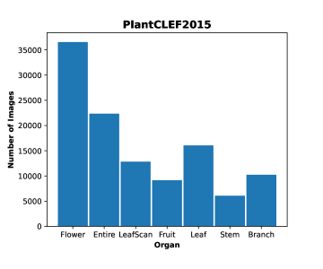
Figure 1: Plant Organ Distributions in PlantCLEF2015

This dataset follows a long-tailed distribution, as depicted in Figure 2. This class imbalance in the data underscores the necessity of employing additional techniques to mitigate its potentially adverse effects on model learning. Furthermore, Figure 3 illustrates the distribution of organ images across classes. Notably, a considerable number of classes entirely lack certain organs. This observation highlights the necessity for models to handle missing modalities effectively, necessitating tailored training approaches.

Figure 2: Class Distribution in PlantCLEF2015

Only the relevant organs—leaves, flowers, fruits, and stems—are considered.

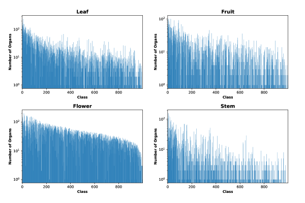
Figure 3: Organ Distribution among Classes in PlantCLEF2015

Logarithmic scale is used to visualize low values.

Moreover, it is evident that flowers, being a discriminative organ (Nhan et al., 2020), are available for most classes, followed by leaves and fruits, although with a noticeable scarcity in many classes. This scarcity is even more pronounced in stems, being the least discriminative and the least available organ across classes. These insights emphasize the importance of addressing the distributional characteristics of organ images within the dataset for robust model training and classification performance.

2.3.1 Data Preprocessing

The original PlantCLEF2015 dataset, in its unprocessed state, lacks suitability for the intended development of our multimodal proposed model. Notably, the dataset contains images stored in varying resolutions and color models without appropriate grouping according to modalities. To rectify these issues and prepare the data and metadata for subsequent model development, essential preprocessing steps have been executed. Further details on these preprocessing steps are provided below.

1. Collecting metadata. Initially, we extract image metadata from the dataset.

2. Standardize images. We convert each image into RGB representation and resize it to the $256\times 256$ resolution. This standardization ensures uniform model input dimensions and minimizes computational load. The adoption of a square shape for resizing is justified by the observation that the average aspect ratio of images in the dataset closely approximates 1.

3. Grouping image indices and corresponding labels. We iterate the metadata to group image indices and labels based on the organs they depict. This is a crucial step for the subsequent modality-wise preprocessing.

4. Filtering small classes. A number of classes in the dataset contain too low a number of images for effective classification, therefore, in this step, we exclude small classes. The classes are filtered in each modality separately because each modality is used individually in step 6, and the proposed multimodal model uses all four modalities simultaneously. A threshold of a minimum of 10 organ images per class is established to include a class in a modality. This filtering results in 302 classes in fruit, 449 in leaf, 862 in flower and 146 in stem modalities, and 956 unique classes in total.

5. Splitting organ indices and corresponding labels. To facilitate model training and evaluation, the data undergoes a stratified split into training, validation, and test sets, with proportions of $60\%:20\%:20\%$. Maintaining consistency with the earlier approaches, splitting is conducted at the modality level.

6. Creating references to unimodal data. Following the observation splitting in step 5, pairs of image indices and labels are organized into data frames to enable loading images and corresponding labels during training, validation and testing of unimodal models (Section 2.2.1).

7. Creating references to multimodal data. In this step, the data is prepared for training the multimodal architecture. To accomplish this, the four modalities must be combined. Each class in the splits generated in step 5 encompasses a varying number of images of distinct organs. A simplistic approach would entail generating all possible combinations of $\textit{flower}\times\textit{leaf}\times\textit{fruit}\times\textit{stem}$ for each class. However, given the unequal distribution of organ images across classes, this would yield numerous similar tuples, potentially burdening computational resources without significant learning benefits. Instead, we only generate $N=max(n_{flower},n_{leaf},n_{fruit},n_{stem})$ random tuples per class, where $n_{m}$ represents the number of images of modality $m$ in the class. We create random tuples for each modality by permuting sequences of modality images and then repeating their elements to match the length of $N$. We store the image indices in the tuple, except when the modality is absent. The resulting tuples are shuffled and, similarly to step 6, together with labels, are stored in a data frame.

2.4 Proposed Model Setup and Configuration

2.4.1 Unimodal Model Training

As mentioned in Section 2.2.1, we train only a classification layer of each unimodal model. This results in 551,612 trainable parameters per model. Each model is trained with identical parameters. We apply an Adam optimizer, initial learning rate of 0.001, utilizing exponential decay of 0.95 every 300 steps during the training of unimodal models. Moreover, models undergo training for 1000 epochs with a batch size of 128 and shuffling. However, we incorporate early stopping with the patience of 10 and the best weight restoration.

To minimize the impact of class imbalance, we employ a weighted cross-entropy loss, where a weight for each class is computed according to the formula:

$$w_{c}=1-\frac{N_{c}}{N}$$ (2)

where $N_{c}$ is the number of instances of a class $c$ within the training data, and $N$ is a total number of instances. Additionally, the L1 and L2 regularizations of $10^{-5}$ are applied. Moreover, label smoothing of 0.1 is applied to the loss.

2.4.2 Multimodal Fusion Architecture Search Execution

During the MFAS algorithm procedure, each multimodal architecture is trained with Adam optimizer, with a learning rate of 0.001 and a weighted cross-entropy loss, with class weights determined according to Equation 2. We fix the number of neurons per fusion layer to 64. Each architecture undergoes training for 2 epochs with a batch size of 128 and shuffling. Given the imbalanced nature of the dataset, we monitor the training progress by checking the F1 macro metric on the validation set. Similar to Perez-Rua et al. (2019), we initialize our temperature scheduler with $t_{max}=10$, $t_{min}=0.2$, and temperature decay $d=4$.

To make models robust to missing modalities (as discussed in Section 2.3), we adopt the multimodal dropout technique proposed by Cheerla and Gevaert (2019). Inspired by a regular dropout, multimodal dropout involves dropping entire modalities during training. This encourages the model to build representations robust to missing modalities. Each modality of a sample is dropped with a similar probability. We utilize a low multimodal dropout rate of 0.125 because many classes are completely devoid of certain modalities.

In this study, we execute the MFAS algorithm for 4 iterations, with 3 progression levels each and set the number of sampled architectures to 50. It is crucial to note that exploring all 1250 initial architectures at the start of the algorithm is time-consuming, so they have been explored in 20 parallel batches. Subsequently, based on the scores obtained, the algorithm has been restarted with the 50 best architectures used as initial ones.

2.4.3 Final Model Training

After the execution of the MFAS algorithm, we select the 10 most performant architectures and train for 100 epochs. Early stopping is employed with a patience of 10, and exponential learning rate decay of 0.95 is applied each epoch. The other hyperparameters remain the same as during the search to determine the best architecture.

Subsequently, we tune the hyperparameters of the best architecture carefully. Initially, the optimal number of neurons per layer is investigated. As suggested by Perez-Rua et al. (2019), small weight matrices are utilized during the algorithm to enhance its speed and reduce memory consumption. However, when focusing on a single architecture, this limitation is no longer applicable. Next, dropouts, various regularization techniques, and other hyperparameters are tested to find an optimal configuration. Finally, the resulting model is trained to completion for 100 epochs with early stopping with a patience of 10. At this stage, the unimodal backbones within it are unfrozen and fine-tuned with a lower learning rate to potentially further enhance performance.

2.5 Model Evaluation

2.5.1 Establishing Baseline

The baseline for the proposed model is established as a late fusion of all unimodal models. This serves as a straightforward approach to fusion, enabling the demonstration that the performance difference between the final model and the baseline is attributed to the unique fusion configuration of the final model.

We implement the late fusion using the averaging strategy, similar to Baltrusaitis et al. (2019). In this approach, the final prediction for an instance $x$ is calculated according to the formula:

$$\hat{y}=\mathop{\text{argmax}}_{y\in Y}p_{\text{avg}}(y|x)$$ (3)

where $y$ represents a class label from the set of all class labels $Y$, and $p_{\text{avg}}$ denotes the average of probabilities from each model. Note that in cases where an instance lacks a modality, the corresponding unimodal model is not involved in the prediction generation process.

2.5.2 Comparison with the Baseline

The evaluation of the proposed model relies on standard performance metrics and comparison against the baseline to determine if the automatic fusion setting of the model leads to improvements. Subsequently, we apply McNemar’s test (Dietterich, 1998) to ascertain if there exists a statistically significant difference between the two models.

To be more specific, in this study, we utilize the following performance metrics:

$$Accuracy=\frac{TP+TN}{TP+TN+FP+FN}$$ (4)

$$Precision=\frac{TP}{TP+FP}$$ (5)

$$Recall=\frac{TP}{TP+FN}$$ (6)

$$F1=2\times\frac{Precision\times Recall}{Precision+Recall}$$ (7)

where with respect to each class, $TP$ (true positives) represents the number of correctly identified instances, $TN$ (true negatives) denotes the number of correctly rejected instances, $FP$ (false positives) signifies the number of incorrectly identified instances, and $FN$ (false negatives) indicates the number of incorrectly rejected instances.

For each class, we compute both micro and macro averages of each metric, except for accuracy. In micro averaging, all $TP$, $TN$, $FP$, and $FN$ values are accumulated before calculating the metric, whereas in macro averaging, a metric is first calculated for each class and then averaged across all classes. The discrepancy between these values provides insight into the performance variation across classes. In conjunction with these metrics, top-5 and top-10 accuracies are also calculated.

2.5.3 Robustness to Missing Modalities

To enable a comparison between unimodal models and multimodal models, we also collect the same metrics discussed in Section 2.5.2 for individual unimodal models. Moreover, to facilitate an understanding of the robustness capabilities of the proposed model in the absence of certain modalities, we collect the mentioned metrics for the proposed model and the baseline on different subsets of modalities.

3 Results

This section presents the findings from our comprehensive evaluation of the proposed model. We have structured our results to provide a clear and systematic presentation under various conditions and compared them to an established baseline.

3.1 Performance of Unimodal Models

After the training procedure (see Section 2.4.1), the unimodal models have been evaluated. Table 1 illustrates the resulting performance metrics.

Modalities:	Flower	Leaf	Fruit	Stem
Accuracy	0.6411	0.5147	0.6759	0.4784
Top-5 accuracy	0.8281	0.7178	0.8416	0.7013
Top-10 accuracy	0.8844	0.7863	0.8895	0.7749
Precisionmicro	0.6411	0.5147	0.6759	0.4784
Precisionmacro	0.6244	0.4532	0.6883	0.4184
Recallmicro	0.6411	0.5147	0.6759	0.4784
Recallmacro	0.5574	0.3815	0.6248	0.3888
F1micro	0.6411	0.5147	0.6759	0.4784
F1macro	0.5671	0.3916	0.6276	0.3814

Table 1: Performance Metrics of Unimodal Models

According to Tabe 1: (i) It is evident that the fruit and flower modalities exhibit higher scores across all metrics compared to leaves and especially stems. This is in line with expectations, considering that stems are the least discriminative organs (Nhan et al., 2020). (ii) Micro metrics demonstrate higher values compared to macro ones. This discrepancy should be attributed to differences in performance among classes. As mentioned in Section 2.3, the dataset is imbalanced, which has affected the overall performance. (iii) Higher macro precision values compared to macro recall suggest that, on average, the models tend to miss correct instances rather than misclassify them. (iv) Relatively high top-$N$ accuracies indicate that the models are typically close to identifying the correct class.

3.2 Finding Final Architecture

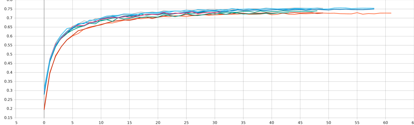
Figure 4: Validation Accuracies of Sampled Architectures per Epoch

As a result of the search to find the best fusion point, 10 best configurations are sampled. These configurations are depicted in Table 2. Consequently, we train the configurations, as described in Section 2.4.3. Figure 4 shows that all architectures converged to approximately 73%–75% validation accuracy. Although showing minimal difference compared to other candidates, the best architecture reported by the MFAS algorithm (1st in Table 2) demonstrated to be the most effective during this test, achieving a validation accuracy of 75.6%. Therefore, we have selected this architecture to proceed with hyperparameter tuning.

Nr.	1st fusion	2nd fusion	3rd fusion	F1macro
1	$\sigma({\color[rgb]{0,0,1}R11},{\color[rgb]{1,.5,0}R1},{\color[rgb]{0,.5,.5}A},{\color[rgb]{.75,0,.25}R1})$	$\sigma({\color[rgb]{0,0,1}R6},{\color[rgb]{1,.5,0}R1},{\color[rgb]{0,.5,.5}A},{\color[rgb]{.75,0,.25}R6})$	$ReLU({\color[rgb]{0,0,1}O},{\color[rgb]{1,.5,0}R11},{\color[rgb]{0,.5,.5}O},{\color[rgb]{.75,0,.25}O})$	0.4652
2	$\sigma({\color[rgb]{0,0,1}R11},{\color[rgb]{1,.5,0}R6},{\color[rgb]{0,.5,.5}R6},{\color[rgb]{.75,0,.25}R11})$	$ReLU({\color[rgb]{0,0,1}R11},{\color[rgb]{1,.5,0}R11},{\color[rgb]{0,.5,.5}O},{\color[rgb]{.75,0,.25}A})$	$ReLU({\color[rgb]{0,0,1}O},{\color[rgb]{1,.5,0}O},{\color[rgb]{0,.5,.5}R11},{\color[rgb]{.75,0,.25}O})$	0.4634
3	$ReLU({\color[rgb]{0,0,1}R1},{\color[rgb]{1,.5,0}R1},{\color[rgb]{0,.5,.5}A},{\color[rgb]{.75,0,.25}R6})$	$\sigma({\color[rgb]{0,0,1}A},{\color[rgb]{1,.5,0}R11},{\color[rgb]{0,.5,.5}R11},{\color[rgb]{.75,0,.25}R1})$	$ReLU({\color[rgb]{0,0,1}O},{\color[rgb]{1,.5,0}O},{\color[rgb]{0,.5,.5}R11},{\color[rgb]{.75,0,.25}O})$	0.4547
4	$ReLU({\color[rgb]{0,0,1}A},{\color[rgb]{1,.5,0}R6},{\color[rgb]{0,.5,.5}O},{\color[rgb]{.75,0,.25}R1})$	$ReLU({\color[rgb]{0,0,1}R11},{\color[rgb]{1,.5,0}R11},{\color[rgb]{0,.5,.5}O},{\color[rgb]{.75,0,.25}A})$	$ReLU({\color[rgb]{0,0,1}O},{\color[rgb]{1,.5,0}O},{\color[rgb]{0,.5,.5}R11},{\color[rgb]{.75,0,.25}O})$	0.4525
5	$ReLU({\color[rgb]{0,0,1}R11},{\color[rgb]{1,.5,0}R6},{\color[rgb]{0,.5,.5}R11},{\color[rgb]{.75,0,.25}R6})$	$\sigma({\color[rgb]{0,0,1}R1},{\color[rgb]{1,.5,0}A},{\color[rgb]{0,.5,.5}O},{\color[rgb]{.75,0,.25}R1})$	$ReLU({\color[rgb]{0,0,1}O},{\color[rgb]{1,.5,0}R11},{\color[rgb]{0,.5,.5}O},{\color[rgb]{.75,0,.25}O})$	0.4463
6	$ReLU({\color[rgb]{0,0,1}R11},{\color[rgb]{1,.5,0}R6},{\color[rgb]{0,.5,.5}R1},{\color[rgb]{.75,0,.25}R11})$	$ReLU({\color[rgb]{0,0,1}R11},{\color[rgb]{1,.5,0}R11},{\color[rgb]{0,.5,.5}O},{\color[rgb]{.75,0,.25}A})$	$ReLU({\color[rgb]{0,0,1}O},{\color[rgb]{1,.5,0}O},{\color[rgb]{0,.5,.5}R11},{\color[rgb]{.75,0,.25}O})$	0.4413
7	$\sigma({\color[rgb]{0,0,1}O},{\color[rgb]{1,.5,0}R1},{\color[rgb]{0,.5,.5}R6},{\color[rgb]{.75,0,.25}R6})$	$\sigma({\color[rgb]{0,0,1}R6},{\color[rgb]{1,.5,0}O},{\color[rgb]{0,.5,.5}O},{\color[rgb]{.75,0,.25}O})$	$ReLU({\color[rgb]{0,0,1}O},{\color[rgb]{1,.5,0}R11},{\color[rgb]{0,.5,.5}A},{\color[rgb]{.75,0,.25}R1})$	0.4376
8	$\sigma({\color[rgb]{0,0,1}R11},{\color[rgb]{1,.5,0}R6},{\color[rgb]{0,.5,.5}A},{\color[rgb]{.75,0,.25}R1})$	$ReLU({\color[rgb]{0,0,1}O},{\color[rgb]{1,.5,0}R1},{\color[rgb]{0,.5,.5}R6},{\color[rgb]{.75,0,.25}R1})$	$ReLU({\color[rgb]{0,0,1}O},{\color[rgb]{1,.5,0}R11},{\color[rgb]{0,.5,.5}O},{\color[rgb]{.75,0,.25}O})$	0.4362
9	$ReLU({\color[rgb]{0,0,1}R11},{\color[rgb]{1,.5,0}O},{\color[rgb]{0,.5,.5}R11},{\color[rgb]{.75,0,.25}O})$	$\sigma({\color[rgb]{0,0,1}R6},{\color[rgb]{1,.5,0}O},{\color[rgb]{0,.5,.5}O},{\color[rgb]{.75,0,.25}O})$	$ReLU({\color[rgb]{0,0,1}O},{\color[rgb]{1,.5,0}R11},{\color[rgb]{0,.5,.5}A},{\color[rgb]{.75,0,.25}R1})$	0.4353
10	$\sigma({\color[rgb]{0,0,1}R11},{\color[rgb]{1,.5,0}R1},{\color[rgb]{0,.5,.5}A},{\color[rgb]{.75,0,.25}R1})$	$ReLU({\color[rgb]{0,0,1}O},{\color[rgb]{1,.5,0}R1},{\color[rgb]{0,.5,.5}R6},{\color[rgb]{.75,0,.25}R11})$	$ReLU({\color[rgb]{0,0,1}O},{\color[rgb]{1,.5,0}R11},{\color[rgb]{0,.5,.5}O},{\color[rgb]{.75,0,.25}O})$	0.4341
$ReLU$ and $\sigma$ denote activation functions of fusion layers, whereas their parameters denote
layers fused from flower, leaf, fruit and stem unimodal models respectively. $A$ – first activation,
$O$ – global average pooling on the top of a model, $RN$ – $N$-th inverted residual block.
F1macro values have been achieved by models for 2 epochs during the search (Section 2.4.2).

Table 2: Best Configurations Sampled by MFAS

3.3 Final Model

To train the final model, we adjust various hyperparameters of the first architecture from Table 2. The number of neurons per fusion layer is increased to 512, and to enhance generalization, dropout rates of 0.1, 0.2, 0.2, and 0.1 are set for the fusion layers and the classification layer, respectively. Additionally, we apply L2 regularization of $10^{-5}$, weight decay of 0.01, and label smoothing of 0.02. Batch normalization was added after each fusion layer.

With all the aforementioned changes, the model is set up for training for 100 epochs, with Adam optimizer, initial learning rate of 0.001 with exponential decay of 0.95 per epoch, and early stopping with patience of 10, resulting in a validation accuracy of 81.72%, as shown in Figure 5. To further enhance performance, we fine-tune the resulting model by unfreezing unimodal base models. To do so, all hyperparameters are retained, except for the initial learning rate, which has been replaced with a value of $10^{-4}$ to prevent erasing previously learned knowledge. As a result, as shown in Figure 5, the validation accuracy increases to 83.45%.

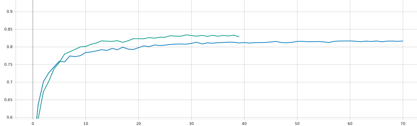
Figure 5: Validation Accuracy of Final Model per Epoch

Blue – before fine-tuning, green – after fine-tuning.

3.4 Comparison with the Baseline

We collect the performance metrics of the proposed model and the baseline on the test set, which are displayed in Table 3.

	Proposed Model	Baseline
Accuracy	0.8348	0.7241
Top-5 accuracy	0.9418	0.8891
Top-10 accuracy	0.9604	0.9293
Precisionmicro	0.8348	0.7241
Precisionmacro	0.8074	0.7220
Recallmicro	0.8348	0.7241
Recallmacro	0.7739	0.6408
F1micro	0.8348	0.7241
F1macro	0.7751	0.6529

Table 3: Performance Metrics of Proposed Model and Baseline

These results indicate that the proposed model significantly outperforms the baseline across all explored metrics and suggest that our automated fused model is substantially more effective and reliable in plant classification on the given dataset compared to a straightforward late fusion approach. The improvement is particularly notable in the macro recall, where it reaches +0.1331. This suggests that the proposed model misses the correct instances of a class significantly less frequently than the baseline. Conversely, a more modest improvement is observed in macro precision, where it reaches +0.0854. Interestingly, the difference between micro and macro precision implies that the baseline demonstrates relatively high precision when positively classifying instances of rare classes.

3.4.1 McNemar’s Test Results

We also conduct McNemar’s test to compare the performance of two multimodal plant classifiers, the proposed model and the baseline. The contingency table of model predictions is provided in Table 4. The test yielded a statistic $\chi^{2}_{1}=617.53$, which is statistically significant ($p<0.001$), indicating a significant difference in performance metrics between our proposed model and the baseline.

$n_{00}$: 1161	$n_{01}$: 248
$n_{10}$: 1192	$n_{11}$: 5927

Table 4: Contingency Table of Proposed Model and Baseline

3.5 Comparison with Unimodal Models

One can observe from Table 1 and Table 3 that both our proposed model and late fusion significantly outperform each individual unimodal model. However, these observations do not fully consider the fact that the unimodal models are evaluated on isolated unimodal datasets, whereas the multimodal model is evaluated on a multimodal dataset containing missing modalities and duplications.

To address this and in order to have a fair comparison, we evaluate both our proposed model and the unimodal models on isolated modalities from the multimodal dataset. The results of this comparison are presented in Table 5.

	Unimodal Model	Proposed Model
Flower	0.5638	0.4647
Leaf	0.3755	0.2094
Fruit	0.6158	0.4166
Stem	0.3622	0.2279

Table 5: Comparison of F1_macro of Proposed and Unimodal Models on Individual Modalities

The metrics presented in Table 5 account for the absence of target modalities by including only those dataset instances that contain the required modality. While the multimodal model demonstrates commendable performance across individual modalities, it generally underperforms compared to the unimodal models when restricted to using only one modality. In detail, interestingly, the performance gap between the multimodal and unimodal models is notably smaller for the flower modality. This might be influenced by the abundance of flower examples in the dataset, providing a richer training environment. Additionally, factors such as the number of classes within each modality and the inherent discriminative capacity of the organs likely affect the performance metrics of the multimodal model. The observed lower performances could stem from a deficiency in data, whereas discrepancies with the unimodal models might be attributed to interference from other modal components within the multimodal system. Given these observations, it is expected that models specifically trained on individual modalities would surpass the performance of a multimodal model when only a single modality is accessible.

3.6 Robustness to Missing Modalities

While cases where a single or all organs are available, represent two extremes, there exists a considerable number of image combinations within the dataset where 2–3 modalities are available. Therefore, it is essential to evaluate the performance of our proposed model and the baseline on all possible subsets of 2–3 modalities. We present the results of this evaluation in Table 6. Similarly to Table 5, it is important to note that the metrics in Table 6 account for the absence of target modalities by excluding instances that miss any of the required modalities.

Modalities	Proposed Model	Baseline
Flower, Leaf	0.6236	0.5102
Flower, Fruit	0.6233	0.5907
Flower, Stem	0.4562	0.4361
Leaf, Fruit	0.6097	0.5818
Leaf, Stem	0.5356	0.4603
Fruit, Stem	0.6142	0.5382
Flower, Fruit, Leaf	0.7816	0.5985
Flower, Stem, Leaf	0.7332	0.5261
Flower, Fruit, Stem	0.6079	0.5416
Leaf, Fruit, Stem	0.7638	0.6143

Table 6: Comparison of F1_macro of Proposed and Baseline Models on Subsets of Modalities

According to Table 5: (i) Across all cases, the proposed model consistently outperforms the baseline, indicating that our approach is superior to naive averaging in any multimodal configuration. (ii) In the cases of leaf–stem and fruit–stem, the latter exhibits higher performance in both models. This suggests that the discriminative features of fruits outweigh the representativeness of leaves. This observation aligns with the metrics presented in Table 1. (iii) An interesting observation arises from the comparison between the combinations of flower–leaf versus flower–fruit. It is notable that the former combination exhibits slightly better performance over the latter in the proposed model, whereas the opposite trend is observed in the baseline. This empirical evidence supports the notion put forth by Nhan et al. (2020) that flowers are the most discriminative organ. However, this discriminativeness seems to be insufficient when all modalities contribute equally to the final prediction, as in late fusion. In such cases, late fusion may favor another highly distinctive organ, such as fruits. In contrast, our model, employing a sophisticated, learned prediction strategy, demonstrates more robustness in either situation. It appears to prefer leaves, as they are more numerous, and the model makes fewer biased assumptions about the equality of modalities. Consequently, it more effectively analyzes combinations of modalities, leading to improved performance across various configurations. (iv) Additionally, the results suggest that stems may have the least positive impact on performance. This finding aligns with the observations in (Nhan et al., 2020), which argue that stems are the least discriminative organ. However, this particular conclusion should be interpreted with caution, as stems are also the least available organ in the dataset.

Overall, the proposed model demonstrates robustness to missing modalities. However, the availability of data remains a bottleneck for performance. Evidently, the less discriminative organs are, the more training data is needed to achieve higher results. This underscores the importance of data availability and diversity in training robust multimodal models.

4 Discussion

Our proposed multimodal DL model, leveraging plant organ images fused via the MFAS algorithm, proves highly effective in automating plant classification, reaching an accuracy of 83.48%. Its performance significantly surpasses the defined baseline and outperforms state-of-the-art models in various aspects with comparable settings, as summarized in Table 7. To be more specific, for example, Ghazi et al. (2017) employed all organs from the PlantCLEF2015 dataset. Despite utilizing larger and more sophisticated classifiers, along with advanced scoring methods, they achieved an accuracy of 80.18%. Despite our architecture being relatively small (6 million parameters), the incorporation of multimodal fusion allowed us to outperform their model, highlighting the strength of multimodality and the advantages of an optimized fusion strategy of our proposed method. Similarly, de Lutio et al. (2021) sampled a large dataset comprising 56608 images of 977 species from the iNaturalist database. Utilizing images and spatio-temporal context, their multimodal model achieved accuracies of 79.12% without satellite imagery and 79.73% with it. While a direct comparison is challenging due to the use of different datasets, our approach, incorporating various organ modalities, yielded higher results. Furthermore, Lee et al. (2018), also using the PlantCLEF2015 dataset, achieved an accuracy of 68.5%. Ge et al. (2016) and Nguyen et al. (2016) extracted flower species from the PlantCLEF2015 dataset and achieved an accuracy of 52.1% and 67.45% respectively. All these results are significantly lower than ours, underscoring the effectiveness of our approach.

In addition to these comparisons, our proposed method demonstrates robustness to missing modalities, as evidenced by its comparison with the baseline in Section 3.6. Even in scenarios where only a single modality is available, the model’s performance is reasonably close to that of standalone unimodal models.

Study	Dataset	Classes	Modalities	Method	Accuracy
Proposed method	PlantCLEF2015	956	Flower, Leaf, Fruit, Stem	MFAS using MobileNetV3Small	83.45%
de Lutio et al. (2021)	iNaturalist	977	Plant images, metadata, satellite imagery	ResNet	79.73%
Lee et al. (2018)	PlantCLEF2015	1000	Plant organ	HGO-CNN + Plant-StructNet	68.5%
Ghazi et al. (2017)	PlantCLEF2015	1000	Plant organ	GoogleNet + VGG	80.18 %
Nguyen et al. (2016)	PlantCLEF2015	967	Flower	GoogleNet	67.45%
Ge et al. (2016)	PlantCLEF2015	967	Flower	MixDCNN	52.1%

Table 7: Comparison with Similar Studies

Extending the related work, we might observe some other multimodal studies achieving better results; however, this is often due to less complex experimental setups. For instance, Zhang et al. (2012) achieved an accuracy of 93.23%, but on a dataset comprising very small images. Similarly, Liu et al. (2016) achieved top-1, top-5 and top-10 accuracies of 71.8%, 91.2% and 96.4% without geographical data, and 50%, 100% and 100% with it, respecively. However, their dataset included only 50 species, each with 10 leaf and 10 flower images, collected in controlled conditions. Likewise, Salve et al. (2018) demonstrated a high GAR score, but their dataset consisted of only 60 species with 10 images each, all collected in laboratory conditions. Furthermore, Nhan et al. (2020) achieved a maximum 98.8% accuracy by utilizing all PlantCLEF2015 organs and 91.4–98.0% depending on model configurations, on only flowers, leaves, fruits, and stems, but they sampled only 50 species from the dataset, each containing all organs, thus not experiencing missing modalities as we did.

5 Conclusions

This study has addressed a critical task in agriculture and ecology: plant classification. By proposing a novel approach in this domain – a multimodal DL model utilizing four plant organs automatically fused via the MFAS algorithm, the study has demonstrated high performance, outperforming other state-of-the-art models despite the smaller size of the model. This underscores the effectiveness of multimodality and an optimal fusion strategy. Moreover, the model exhibits robustness to missing modalities, even when only a single modality is available. We believe that this proposed approach opens up a promising direction in plant classification research. This highlights the need for further exploration through the development of more sophisticated algorithms capable of handling larger numbers of species, thereby unlocking the full potential of this approach. A future research could also consider incorporating a multimodal fusion of vision transformers instead of CNNs for plant classification.

References

- Baltrusaitis et al. (2019) Baltrusaitis, T., Ahuja, C., Morency, L.P., 2019. Multimodal machine learning: A survey and taxonomy. IEEE Trans. Pattern Anal. Mach. Intell. 41, 423–443. URL: https://doi.org/10.1109/TPAMI.2018.2798607, doi:10.1109/TPAMI.2018.2798607.
- Barua et al. (2023) Barua, A., Ahmed, M.U., Begum, S., 2023. A systematic literature review on multimodal machine learning: Applications, challenges, gaps and future directions. IEEE Access 11, 14804–14831. doi:10.1109/ACCESS.2023.3243854.
- Beikmohammadi and Faez (2018) Beikmohammadi, A., Faez, K., 2018. Leaf classification for plant recognition with deep transfer learning, in: 2018 4th Iranian Conference on Signal Processing and Intelligent Systems (ICSPIS), pp. 21–26. doi:10.1109/ICSPIS.2018.8700547.
- Beikmohammadi et al. (2022) Beikmohammadi, A., Faez, K., Motallebi, A., 2022. Swp-leafnet: A novel multistage approach for plant leaf identification based on deep cnn. Expert Systems with Applications 202, 117470. URL: https://www.sciencedirect.com/science/article/pii/S0957417422008016, doi:https://doi.org/10.1016/j.eswa.2022.117470.
- Boulahia et al. (2021) Boulahia, S.Y., Amamra, A., Madi, M.R., Daikh, S., 2021. Early, intermediate and late fusion strategies for robust deep learning-based multimodal action recognition. Machine Vision and Applications 32, 121.
- Cheerla and Gevaert (2019) Cheerla, A., Gevaert, O., 2019. Deep learning with multimodal representation for pancancer prognosis prediction. Bioinformatics 35, i446–i454.
- de Lutio et al. (2021) de Lutio, R., She, Y., D’Aronco, S., Russo, S., Brun, P., Wegner, J.D., Schindler, K., 2021. Digital taxonomist: Identifying plant species in community scientists’ photographs. ISPRS Journal of Photogrammetry and Remote Sensing 182, 112–121. URL: https://www.sciencedirect.com/science/article/pii/S0924271621002641, doi:https://doi.org/10.1016/j.isprsjprs.2021.10.002.
- Dietterich (1998) Dietterich, T.G., 1998. Approximate statistical tests for comparing supervised classification learning algorithms. Neural computation 10, 1895–1923.
- Dyrmann et al. (2016) Dyrmann, M., Karstoft, H., Midtiby, H.S., 2016. Plant species classification using deep convolutional neural network. Biosystems engineering 151, 72–80.
- Elsken et al. (2019) Elsken, T., Metzen, J.H., Hutter, F., 2019. Neural architecture search: A survey. Journal of Machine Learning Research 20, 1–21.
- Espejo-Garcia et al. (2020) Espejo-Garcia, B., Mylonas, N., Athanasakos, L., Fountas, S., Vasilakoglou, I., 2020. Towards weeds identification assistance through transfer learning. Computers and Electronics in Agriculture 171, 105306.
- Gao et al. (2018) Gao, J., Nuyttens, D., Lootens, P., He, Y., Pieters, J.G., 2018. Recognising weeds in a maize crop using a random forest machine-learning algorithm and near-infrared snapshot mosaic hyperspectral imagery. Biosystems engineering 170, 39–50.
- Ge et al. (2016) Ge, Z., Bewley, A., McCool, C., Corke, P., Upcroft, B., Sanderson, C., 2016. Fine-grained classification via mixture of deep convolutional neural networks, in: 2016 IEEE Winter Conference on Applications of Computer Vision (WACV), IEEE. pp. 1–6.
- Ghazi et al. (2017) Ghazi, M.M., Yanikoglu, B., Aptoula, E., 2017. Plant identification using deep neural networks via optimization of transfer learning parameters. Neurocomputing 235, 228–235.
- Ghosh et al. (2022) Ghosh, S., Singh, A., Jhanjhi, N., Masud, M., Aljahdali, S., et al., 2022. Svm and knn based cnn architectures for plant classification. Computers, Materials & Continua 71.
- Haichen et al. (2021) Haichen, J., Qingrui, C., Zheng Guang, L., 2021. Weeds and crops classification using deep convolutional neural network, in: Proceedings of the 3rd International Conference on Control and Computer Vision, Association for Computing Machinery, New York, NY, USA. p. 40–44. URL: https://doi.org/10.1145/3425577.3425585, doi:10.1145/3425577.3425585.
- Hoang Trong et al. (2020) Hoang Trong, V., Gwang-hyun, Y., Thanh Vu, D., Jin-young, K., 2020. Late fusion of multimodal deep neural networks for weeds classification. Computers and Electronics in Agriculture 175, 105506. URL: https://www.sciencedirect.com/science/article/pii/S0168169919319799, doi:https://doi.org/10.1016/j.compag.2020.105506.
- Howard et al. (2019) Howard, A., Sandler, M., Chu, G., Chen, L.C., Chen, B., Tan, M., Wang, W., Zhu, Y., Pang, R., Vasudevan, V., et al., 2019. Searching for mobilenetv3, in: Proceedings of the IEEE/CVF international conference on computer vision, pp. 1314–1324.
- Joly et al. (2015) Joly, A., Goëau, H., Glotin, H., Spampinato, C., Bonnet, P., Vellinga, W.P., Planqué, R., Rauber, A., Palazzo, S., Fisher, B., et al., 2015. Lifeclef 2015: multimedia life species identification challenges, in: Experimental IR Meets Multilinguality, Multimodality, and Interaction: 6th International Conference of the CLEF Association, CLEF’15, Toulouse, France, September 8-11, 2015, Proceedings 6, Springer. pp. 462–483.
- Kaya et al. (2019) Kaya, A., Keceli, A.S., Catal, C., Yalic, H.Y., Temucin, H., Tekinerdogan, B., 2019. Analysis of transfer learning for deep neural network based plant classification models. Computers and Electronics in Agriculture 158, 20–29. URL: https://www.sciencedirect.com/science/article/pii/S0168169918315308, doi:https://doi.org/10.1016/j.compag.2019.01.041.
- Kolhar and Jagtap (2021) Kolhar, S., Jagtap, J., 2021. Plant trait estimation and classification studies in plant phenotyping using machine vision - a review. Information Processing in Agriculture 10. doi:10.1016/j.inpa.2021.02.006.
- Lee et al. (2018) Lee, S.H., Chan, C.S., Remagnino, P., 2018. Multi-organ plant classification based on convolutional and recurrent neural networks. IEEE Transactions on Image Processing 27, 4287–4301.
- Liu et al. (2016) Liu, J.C., Chiang, C.Y., Chen, S., 2016. Image-based plant recognition by fusion of multimodal information, in: 2016 10th International Conference on Innovative Mobile and Internet Services in Ubiquitous Computing (IMIS), pp. 5–11. doi:10.1109/IMIS.2016.60.
- Liu et al. (2022) Liu, K.H., Yang, M.H., Huang, S.T., Lin, C., 2022. Plant species classification based on hyperspectral imaging via a lightweight convolutional neural network model. Frontiers in Plant Science 13. doi:10.3389/fpls.2022.855660.
- Liu et al. (2021) Liu, Y., Sun, Y., Xue, B., Zhang, M., Yen, G.G., Tan, K.C., 2021. A survey on evolutionary neural architecture search. IEEE transactions on neural networks and learning systems 34, 550–570.
- Meshram et al. (2021) Meshram, V., Patil, K., Meshram, V., Hanchate, D., Ramkteke, S., 2021. Machine learning in agriculture domain: A state-of-art survey. Artificial Intelligence in the Life Sciences 1, 100010.
- Nguyen et al. (2016) Nguyen, T.T.N., Le, V., Le, T., Hai, V., Pantuwong, N., Yagi, Y., 2016. Flower species identification using deep convolutional neural networks, in: AUN/SEED-Net Regional Conference for Computer and Information Engineering.
- Nhan et al. (2020) Nhan, N.T.T., Le, T.L., Hai, V., 2020. Do we need multiple organs for plant identification?, in: 2020 International Conference on Multimedia Analysis and Pattern Recognition (MAPR), pp. 1–6. doi:10.1109/MAPR49794.2020.9237787.
- Perez-Rua et al. (2018) Perez-Rua, J.M., Baccouche, M., Pateux, S., 2018. Efficient progressive neural architecture search .
- Perez-Rua et al. (2019) Perez-Rua, J.M., Vielzeuf, V., Pateux, S., Baccouche, M., Jurie, F., 2019. Mfas: Multimodal fusion architecture search, in: 2019 IEEE/CVF Conference on Computer Vision and Pattern Recognition (CVPR), pp. 6959–6968. doi:10.1109/CVPR.2019.00713.
- Saleem et al. (2018) Saleem, G., Akhtar, M., Ahmed, N., Qureshi, W., 2018. Automated analysis of visual leaf shape features for plant classification. Computers and Electronics in Agriculture 157, 270–280. doi:10.1016/j.compag.2018.12.038.
- Salve et al. (2018) Salve, P., Yannawar, P., Sardesai, M.M., 2018. Multimodal plant recognition through hybrid feature fusion technique using imaging and non-imaging hyper-spectral data. Journal of King Saud University - Computer and Information Sciences 34. doi:10.1016/j.jksuci.2018.09.018.
- Sun et al. (2022) Sun, X., Li, G., Qu, P., Xie, X., Pan, X., Zhang, W., 2022. Research on plant disease identification based on cnn. Cognitive Robotics 2, 155–163.
- Tan et al. (2020) Tan, J.w., Chang, S.W., Abdul-Kareem, S., Yap, H.J., Yong, K.T., 2020. Deep learning for plant species classification using leaf vein morphometric. IEEE/ACM Transactions on Computational Biology and Bioinformatics 17, 82–90. doi:10.1109/TCBB.2018.2848653.
- Umamageswari et al. (2023) Umamageswari, A., Bharathiraja, N., Irene, D.S., 2023. A novel fuzzy c-means based chameleon swarm algorithm for segmentation and progressive neural architecture search for plant disease classification. ICT Express 9, 160–167.
- Wang et al. (2022) Wang, Y., Chen, Y., Wang, D., 2022. Recognition of multi-modal fusion images with irregular interference. PeerJ Computer Science 8, e1018.
- Wäldchen et al. (2018) Wäldchen, J., Rzanny, M., Seeland, M., Mäder, P., 2018. Automated plant species identification—trends and future directions. PLOS Computational Biology 14, 1–19. URL: https://doi.org/10.1371/journal.pcbi.1005993, doi:10.1371/journal.pcbi.1005993.
- Xu et al. (2021) Xu, Z., So, D.R., Dai, A.M., 2021. Mufasa: Multimodal fusion architecture search for electronic health records, in: Proceedings of the AAAI Conference on Artificial Intelligence, pp. 10532–10540.
- Zhang et al. (2020) Zhang, C., Yang, Z., He, X., Deng, L., 2020. Multimodal intelligence: Representation learning, information fusion, and applications. IEEE Journal of Selected Topics in Signal Processing PP, 1–1. doi:10.1109/JSTSP.2020.2987728.
- Zhang et al. (2012) Zhang, S.W., Zhao, M.R., Wang, X.F., 2012. Plant classification based on multilinear independent component analysis, in: Huang, D.S., Gan, Y., Gupta, P., Gromiha, M.M. (Eds.), Advanced Intelligent Computing Theories and Applications. With Aspects of Artificial Intelligence, Springer Berlin Heidelberg, Berlin, Heidelberg. pp. 484–490.
- Zhou et al. (2021) Zhou, J., Li, J., Wang, C., Wu, H., Zhao, C., Teng, G., 2021. Crop disease identification and interpretation method based on multimodal deep learning. Comput. Electron. Agric. 189. URL: https://doi.org/10.1016/j.compag.2021.106408, doi:10.1016/j.compag.2021.106408.