∎
Università del Piemonte Orientale
22email: lidia.aceto@uniupo.it 33institutetext: L. Gemignani 44institutetext: Dipartimento di Informatica
Università di Pisa
44email: luca.gemignani@unipi.it
Computing the Action of the Generating Function of Bernoulli Polynomials on a Matrix with An Application to Non-local Boundary Value Problems
Abstract
This paper deals with efficient numerical methods for computing the action of the generating function of Bernoulli polynomials, say , on a typically large sparse matrix. This problem occurs when solving some non-local boundary value problems. Methods based on the Fourier expansion of have already been addressed in the scientific literature. The contribution of this paper is twofold. First, we place these methods in the classical framework of Krylov-Lanczos (polynomial-rational) techniques for accelerating Fourier series. This allows us to apply the convergence results developed in this context to our function. Second, we design a new acceleration scheme. Some numerical results are presented to show the effectiveness of the proposed algorithms.
Keywords:
Rational approximation of Fourier Series Convergence Acceleration Matrix FunctionsMSC:
15A60 65F601 Introduction
In this work we are interested in the approximation of the function
| (1.1) |
which acts on a typically large sparse matrix. As known, this function is the generating function of Bernoulli polynomials i.e.
| (1.2) |
see e.g. Abramowitz , which are very important in various fields of mathematics and, in particular, are intimately connected to differential equations. For example, recall that in a finite-dimensional setting in Boito1 it is proved that for a given matrix and a given vector the non-local boundary value problem (BVP)
| (1.3) | |||
| (1.4) |
admits as unique solution
| (1.5) |
More general differential problems can also be reduced into the form (1.3), (1.4) by the application of semidiscretization-in-space schemes.
BVPs with special non-local boundary conditions are ubiquitous in applied sciences and engineering. Integral boundary conditions are encountered in various applications such as population dynamics, blood flow models, chemical engineering and cellular systems (see e.g. Bou ; Mar and the references given therein). Interestingly, such problems are also relevant in control theory for system identification, where the analysis goes back to the work of Bellmann Bell .
Several numerical methods have been developed in Boito1 ; Boito for evaluating the matrix function when is large and possibly sparse. The approach based on (1.2) is unreliable since the formal series uniformly converges only within . By using an ad-hoc technique for the convergence acceleration of a Fourier series, in Boito for the following rational-trigonometric modification of (1.2) has been obtained
| (1.6) |
Hence, by truncating the series on the right to a finite number of terms, say in the same work it has been proposed to consider the family of approximations given by
| (1.7) |
Although it has also been shown that the series on the right side of (1.6) converges uniformly to on every set with and compact sets, both the residual estimates and the exact evaluations of the asymptotic error constants are still missing. Furthermore, although increasing the value of can bring great benefits to improve the convergence rate of (1.6), computing the polynomial term of can be prone to numerical instabilities whenever has eigenvalues of large magnitude Boito3 .
This work aims to fill these gaps. The starting point is the derivation of the formula (1.6) in a more general framework for the development of acceleration methods for ordinary Fourier series, which in Pogh is called the Krylov-Lanczos approximation, since this approach was originally proposed by Krylov Krylov and Lanczos Lanczos . The term Krylov-Lanczos approximation denotes a class of methods for accelerating trigonometric series of a non-periodic function by polynomial corrections that represent discontinuities of the function and some of its first derivatives. A classical approach among these methods is the Lanczos representation of functions in terms of Bernoulli polynomials and trigonometric series Lanczos ; Lyn . It is shown that this approach, applied to the periodic extension of , leads to the expansion (1.6). The result allows us to adapt the techniques and tools developed in the general framework for the analysis of the function . Specifically, we derive estimates of the residual error in -norm and for pointwise convergence in the regions far from the discontinuities at the endpoints. Furthermore, we develop an alternative acceleration strategy for which replaces the polynomial term in (1.6) with a suitable rational function expressed in a convenient form as sum of ratios.
The paper is organized as follows. In Section 2 we derive the expansion formula (1.6) in the framework of Lanczos representation. In Section 3 we adjust known error estimates for the Lanczos approximation to the function by devising a suitable scheme for evaluating the pointwise convergence in regions away from the discontinuities. In Section 4 we show that this scheme indeeed yields an effective acceleration scheme involving only the manipulation of rational functions. In Section 5 we illustrate the effectiveness of this scheme by numerical experiments related with the solution of a non-local BVP of type (1.3)-(1.4). Finally, conclusions and future work are drawn in Section 6.
2 Lanczos Acceleration of Fourier Expansions
Suppose we set a value for since is analytic over the unit interval, it can be expanded into Fourier series of and we get
the coefficients that occur in this series (Fourier coefficients) are given by
and through the real and imaginary parts of
From the evaluation of the latter integral it therefore follows that
| (2.8) |
Since is non-periodic, the use of the Fourier series has a computational disadvantage, i.e. the series can converge very slowly.
In (Boito, , Lemma 1), the authors developed methods to accelerate the convergence of (2.8) by using relations expressing Bernoulli polynomials by appropriate numerical series of sine and cosine. This led to the relationship given in (1.6).
In this section, a derivation of the so-called Lanczos representation for the function is described. This involves expressing in the form
| (2.9) |
where is a polynomial of degree and has Fourier coefficients with a decay of order as Following the results reported in (Lyn, , pp. 82, 83), for any we get
| (2.10) | |||||
| (2.11) |
where is the k-th Bernoulli polynomial and the coefficients and are such that
cfr. (Lyn, , Eqs. (1.14) and (1.20)). By direct calculation it is easily found that
| (2.12) | |||||
Consequently,
| (2.16) |
In addition, observing that
and that we can rewrite (see (2.10))
To establish whether the newly introduced Lanczos representation of recovers the expression found in Boito and reported in (1.6), we set and Obviously,
| (2.17) |
Concerning from (2.16) we have that
| (2.18) |
with
| (2.19) |
Then, it is immediate to verify that the Lanczos representation
agrees with (1.6).
Such concurrence is interesting from both a theoretical and a practical point of view. Indeed, it makes possible to adapt general results for the Lanczos representation of regular functions to the specific expansion (1.6) of . These results include error estimates and the design of alternative acceleration schemes. The corresponding adaptations for are the subject of the next sections.
3 Error Estimate and Convergence
The connection between the function and the Lanczos representations discussed in the previous section is now exploited to derive the error estimate and to perform a convergence analysis.
Denoting by
the truncation to the first terms of (see (2.11)), we may approximate
| (3.20) |
Then, we are able to provide an estimate for the error
| (3.21) | |||||
Theorem 3.1
For a given integer the following estimate holds
| (3.22) |
where is the -norm.
Proof
Following (Barkhudaryan, Theorem 2.1) and using (2.12) we can write
with
Using the Parseval’s identity, we get
This concludes the proof.
Remark 1
It is worth noting in (3.22) the occurrence of the term which can be problematic for convergence in the domain. This observation is confirmed by many experimental results reported in GL which indicate that the more is the size of , the more is the number of terms of (1.6) needed to reach a prescribed accuracy.
When and (3.20) coincides with (1.7). So, we can rewrite the approximation to given in (1.7) as
| (3.23) |
Using these notation, we define the error as
| (3.24) |
From Theorem 3.1 it is immediate to deduce that
In Table 1 we show a numerical illustration of this result with . For a given and we compute the quantity
| (3.25) |
where is estimated using the Mathematica function NIntegrate applied to the partial sum formed by the first terms of the expansion (3). Doubling the number of terms does not change the results. The integrands are highly oscillatory and Mathematica returns partial errors of order . As can be seen, for each considered the computed value is a good approximation of independently of
| 512 | 1024 | 2048 | |
| 1 | |||
| 0.1 | |||
| 10 |
To investigate pointwise convergence in regions away from the discontinuities at the endpoints of the interval , we follow an approach that is based on the results of KW and differs from the approach used in Boito . This approach avoids the use of Bernoulli polynomials by employing rational corrections of the error in order to accelerate its convergence toward zero. More precisely, we consider the first term in (3.21) without considering a constant, namely (see (2.16))
| (3.28) | |||||
| (3.29) |
From the relation
it follows that
Therefore, we obtains that
| (3.30) | |||||
with
| (3.31) |
Notice that is the classical approximation of the second derivative of the function (see (3.28) and (2.16))
| (3.35) |
over the grid , . Since
| (3.39) |
from Taylor expansion we deduce that
which implies
| (3.43) |
Analogously, for the second term in (3.21) we have
| (3.46) | |||||
| (3.47) |
Using the the formula
we obtain that
| (3.48) | |||||
with
| (3.49) |
Again, we observe that is the classical approximation of the second derivative of the function
| (3.53) |
over the grid , . Notice that (3.35) coincides with (3.53) up to a change of parity of . Hence, from (3.43) we find that
| (3.57) |
In this way, we arrive at the following result which describes the behaviour of the error in the interior of the unit interval.
Theorem 3.2
For any setting
we have
where denotes the ceiling function and
4 Acceleration of Convergence
The results reported in Theorem 3.1 and Theorem 3.2 illustrate theoretically the acceleration capabilities of Lanczos approximation.
However, the numerical results shown in Boito3 clearly indicate that the computation of the polynomial term in (1.6) can be prone to numerical instabilities. To circumvent this issue, in this section we investigate the design of different acceleration techniques for evaluating . Our starting point is the observation that the strategy devised in the previous section for the error analysis of the Lanczos representation can be applied from scratch
to the expansion with or very small values of .
Recalling that (see (3.28) and (3.46))
and denoting by
and
from (3.30) and (3.48) we find that for any the error can be expressed as (see (3.58))
with
The process can be iterated in order to accelerate the convergence of the two series in the left hand side of this relation by the multiplication by the factor . In this way, by setting for an integer ,
and
we find that
or, equivalently,
| (4.59) | |||||
Remark 2
At the approximation of reduces to the approximation already given in (3.21) without acceleration, i.e.
The error estimates for the residual can be derived using the same arguments exploited in the proofs of Theorem 3.1 and Theorem 3.2. A global estimate of can be obtained by introducing the penalty factors , , as pursued in Pogh ; Pogh1 . In particular, the error analysis is extended by replacing the term with the modified form for appropriate choices of such penalty factors. The overall process behaves similarly with the only modification being the use of weighted finite difference approximations for the second derivatives.
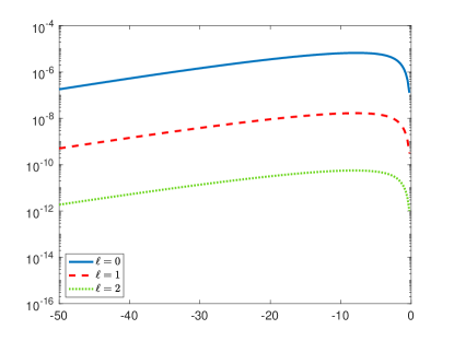
We have performed numerical experiments to test the effectiveness of the proposed acceleration technique. In Figure 1 we illustrate this behavior by drawing the relative error function
for by setting and for different values of and . Our experiments indicate that the method performs quite well for away from the discontinuities and its effectiveness decreases as the value of approaches .

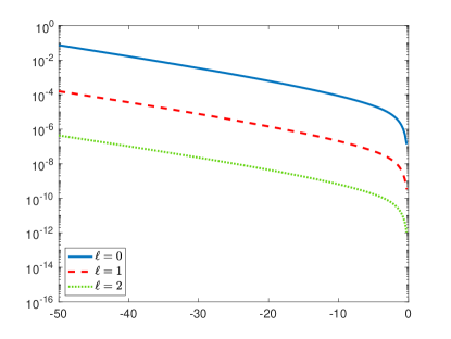
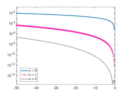
In (a)-(b): In (c)-(d):
If to get reliable algorithm for approximating we must combine our approach with a suitable numerical method for evaluating the exponential function. Indeed, we can rely on the identity
| (4.60) |
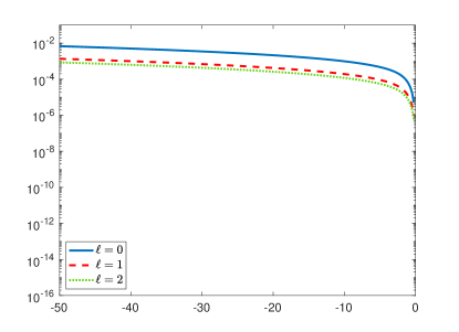
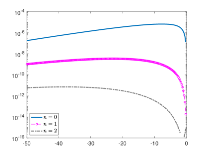
The resulting approach is considered for in Figure 2 where the exponential function is computed using the Matlab built-in function exp.
Another popular method for calculating the exponential is the rational approximation. This tool can be suitable for parallel computations GALSA . For further experiments, we used the rational Chebyshev approximation from for , with and polynomials of degree , where the coefficients of such polynomials up to degree are given in CRV . In this way, we obtain an approximation of , denoted as and defined by
Considering that the rational Chebyshev approximation of has uniform absolute error estimates of the form
cfr. CRV , in Figure 3 we plot the absolute error function
with and for different values of the parameters and


As can be seen by comparing the pictures on the left with those on the right of the figure, the acceleration strategy proposed in this work ( in this example) is more robust than the technique without acceleration () for large input values. To confirm this statement, in the next section we present the results of two numerical tests concerning the computation of with a matrix having a real spectrum located on the negative axis with many eigenvalues of large magnitude. Based on the above results, the use of the acceleration strategy can significantly influence the accuracy of the computation of .
5 Numerical Experiments
In this section we present some experiments starting from the differential problem
| (5.61) |
with the non-local condition
| (5.62) |
As is well known, the numerical solution of such a non-local BVP can be derived by applying the classical method of lines FW . Then one discretizes the one-dimensional operator
by using central differences over the grid of points in the interval and obtains a matrix Thus, the problem (5.61)-(5.62) is reduced to a differential problem of the form (1.3)-(1.4). The derivation of the numerical solution of such a BVP therefore involves the computation of where is the vector with contains the evaluation of on the grid, cfr. (1.5). If we now use with to denote the grid points on the matrix has a tridiagonal structure with non-zero entries
| (5.63) |
When the grid is uniform with stepsize the matrix reduces to with the 1D Laplacian matrix. Note that small values of imply the presence of both large eigenvalues and a large norm of . In light of the Theorem 3.1, the first is a critical fact for the convergence of the approximation (3.20). The second, however, can deteriorate the accuracy of the acceleration strategy. To illustrate these effects, we performed numerical experiments in which we compared for the approximation derived with (3.20) (for such , (3.20) actually reduces to (3.23)) with that in (4.59). As shown in the previous section the latter requires the incorporation of the corrective term . The evaluation of this term boils down to the calculation of quantities
| (5.64) |
and
All these quantities can be obtained from and , , through recurrence relations. Furthermore, is derived from at the cost of additional matrix-by-vector multiplication. The next graph illustrates the computation of the required quantities in (5.64) when .
Therefore, considering that the evaluation of essentially requires the solution of shifted linear systems of the form while the computation of requires solving additional systems, we conclude that for small values of both approximations are comparable in terms of computational cost.
In our numerical experiments we consider as exact solution derived using the MATLAB "backslash" operator and built-in function . We measure the error with
having indicated with the approximate solution provided by one of the two approximations, i.e. and with For short, we denote by
-
Lanc:
-
FastLanc:
For the tridiagonal matrix given in (5.63) and our test suite consists of two experiments:
-
-
Test 1: uniform grid with ;
-
-
Test 2: not uniform grid with
In Table 2 we report the errors provided by the two approximations on a uniform grid for and (i.e. ) when the acceleration is considered. Analogue comparisons for not uniform grid are reported in Table 3. These tables clearly highlight the robustness of the proposed acceleration scheme compared to the strategy based on the use of Lanczos approximation.
| Lanc | ||||||
| 2 | 3 | 4 | 2 | 3 | 4 | |
| 50 | ||||||
| 100 | ||||||
| 200 | ||||||
| FastLanc | ||||||
| 2 | 3 | 4 | 2 | 3 | 4 | |
| 50 | ||||||
| 100 | ||||||
| 200 | ||||||
| Lanc | ||||||
| 2 | 3 | 4 | 2 | 3 | 4 | |
| 50 | ||||||
| 100 | ||||||
| 200 | ||||||
| FastLanc | ||||||
| 2 | 3 | 4 | 2 | 3 | 4 | |
| 50 | ||||||
| 100 | ||||||
| 200 | ||||||
6 Conclusions and Future Work
In this paper we have derived the series expansion of the generating function of Bernoulli polynomials in the framework of the so-called Lanczos acceleration method of Fourier-trigonometric series of smooth non-periodic functions. This is a general method that involves the use of Bernoulli polynomials to accelerate convergence. Our derivation makes it possible to adapt the general error estimates provided for this method to the meromorphic function under consideration, namely the generating function of Bernoulli polynomials. Extensions of this method involving the use of rational functions are also investigated. In particular, we propose a cost-effective acceleration method based on the rational-trigonometric approximation of the residual of the Fourier series. Numerical experiments with finite difference discretizations of differential operators show that our proposed acceleration method outperforms the Lanczos approximation in terms of robustness and accuracy. Future work will focus on the development of an automatic procedure for the selection of the parameters necessary for the construction of the resulting approximations. Another interesting topic is the analysis of Fourier-Padé approximation methods of the residual. Such methods can be very effective when combined with efficient scaling and squaring techniques. The development of these methods for the calculation of is still an ongoing research project.
Acknowledgements.
The authors are members of GNCS-INDAM. Lidia Aceto is partially supported by the "INdAM - GNCS Project", codice CUPE53C23001670001. Luca Gemignani is partially supported by European Union - NextGenerationEU under the National Recovery and Resilience Plan (PNRR) - Mission 4 Education and research - Component 2 From research to business - Investment 1.1 Notice Prin 2022 - DD N. 104 2/2/2022, titled Low-rank Structures and Numerical Methods in Matrix and Tensor Computations and their Application, proposal code 20227PCCKZ – CUP I53D23002280006 and by the Spoke 1 “FutureHPC & BigData” of the Italian Research Center on High-Performance Computing, Big Data and Quantum Computing (ICSC) funded by MUR Missione 4 Componente 2 Investimento 1.4: Potenziamento strutture di ricerca e creazione di "campioni nazionali di R&S (M4C2-19 )" - Next Generation EU (NGEU).References
- (1) Abramowitz, M., and I. A. Stegun. 1965. Handbook of Mathematical Functions: With Formulas, Graphs, and Mathematical Tables. Dover Publications.
- (2) Barkhudaryan, A., R. Barkhudaryan, and A. Poghosyan. 2007. “Asymptotic Behavior of Eckhoff’s Method for Fourier Series Convergence Acceleration.” Anal. Theory Appl. 23 (3): 228–42. https://doi.org/10.1007/s10496-007-0228-0.
- (3) Bellman, R. 1966. “A Note on the Identification of Linear Systems.” Proc. Amer. Math. Soc. 17: 68–71. https://doi.org/10.2307/2035062.
- (4) Boito, P., Y. Eidelman, and L. Gemignani. 2018. “Efficient Solution of Parameter-Dependent Quasiseparable Systems and Computation of Meromorphic Matrix Functions.” Numer. Linear Algebra Appl. 25 (6): e2141, 13. https://doi.org/10.1002/nla.2141.
- (5) ———. 2022. “Computing the Reciprocal of a -Function by Rational Approximation.” Adv. Comput. Math. 48 (1): Paper No. 1, 28. https://doi.org/10.1007/s10444-021-09917-z.
- (6) ———. 2024. “Numerical Solution of Nonclassical Boundary Value Problems.”
- (7) Boucherif, A. 2009. “Second-Order Boundary Value Problems with Integral Boundary Conditions.” Nonlinear Anal. 70 (1): 364–71. https://doi.org/10.1016/j.na.2007.12.007.
- (8) Carpenter, A. J., A. Ruttan, and R. S. Varga. 1984. “Extended Numerical Computations on the ‘’ Conjecture in Rational Approximation Theory.” In Rational Approximation and Interpolation (Tampa, Fla., 1983), 1105:383–411. Lecture Notes in Math. Springer, Berlin. https://doi.org/10.1007/BFb0072427.
- (9) Forsythe, George E., and Wolfgang R. Wasow. 2004. Finite-Difference Methods for Partial Differential Equations. Dover Phoenix Editions. Dover Publications, Inc., Mineola, NY.
- (10) Gallopoulos, E., and Y. Saad. 1992. “Efficient Solution of Parabolic Equations by Krylov Approximation Methods.” SIAM J. Sci. Statist. Comput. 13 (5): 1236–64. https://doi.org/10.1137/0913071.
- (11) Gemignani, Luca. 2023. “Efficient Inversion of Matrix -Functions of Low Order.” Appl. Numer. Math. 192: 57–69. https://doi.org/10.1016/j.apnum.2023.05.026.
- (12) Kiefer, J. E., and G. H. Weiss. 1981. “A Comparison of Two Methods for Accelerating the Convergence of Fourier Series.” Comput. Math. Appl. 7 (6): 527–35. https://doi.org/10.1016/0898-1221(81)90036-5.
- (13) Krylov, A. N. 1950. Lekcii o Približennyh Vyčisleniyah. Gosudarstv. Izdat. Tehn.-Teor. Lit., Moscow-Leningrad.
- (14) Lanczos, C. 1966. Discourse on Fourier Series. Hafner Publishing Co., New York.
- (15) Lyness, J. N. 1974. “Computational Techniques Based on the Lanczos Representation.” Math. Comp. 28: 81–123. https://doi.org/10.2307/2005818.
- (16) Mardanov, M. J., Y. A. Sharifov, Y. S. Gasimov, and C. Cattani. 2021. “Non-Linear First-Order Differential Boundary Problems with Multipoint and Integral Conditions.” Fractal and Fractional 5 (1). https://doi.org/10.3390/fractalfract5010015.
- (17) Poghosyan, A. 2011. “On an Auto-Correction Phenomenon of the Krylov-Gottlieb-Eckhoff Method.” IMA J. Numer. Anal. 31 (2): 512–27. https://doi.org/10.1093/imanum/drp043.
- (18) ———. 2013. “On a Fast Convergence of the Rational-Trigonometric-Polynomial Interpolation.” Adv. Numer. Anal., Art. ID 315748, 13. https://doi.org/10.1155/2013/315748.