Learning Analysis of Kernel Ridgeless Regression with Asymmetric Kernel Learning

Abstract

Ridgeless regression has garnered attention among researchers, particularly in light of the “Benign Overfitting” phenomenon, where models interpolating noisy samples demonstrate robust generalization. However, kernel ridgeless regression does not always perform well due to the lack of flexibility. This paper enhances kernel ridgeless regression with Locally-Adaptive-Bandwidths (LAB) RBF kernels, incorporating kernel learning techniques to improve performance in both experiments and theory. For the first time, we demonstrate that functions learned from LAB RBF kernels belong to an integral space of Reproducible Kernel Hilbert Spaces (RKHSs). Despite the absence of explicit regularization in the proposed model, its optimization is equivalent to solving an $\ell_{0}$-regularized problem in the integral space of RKHSs, elucidating the origin of its generalization ability. Taking an approximation analysis viewpoint, we introduce an $l_{q}$-norm analysis technique (with $0<q<1$) to derive the learning rate for the proposed model under mild conditions. This result deepens our theoretical understanding, explaining that our algorithm’s robust approximation ability arises from the large capacity of the integral space of RKHSs, while its generalization ability is ensured by sparsity, controlled by the number of support vectors. Experimental results on both synthetic and real datasets validate our theoretical conclusions.

Keywords: kernel ridgeless regression, approximation analysis, LAB RBF kernel, the integral space of RKHSs, $\ell_{0}$ regularization

1 Introduction

Kernel methods play a foundational role within the machine learning community, and maintain their importance thanks to their interpretability, strong theoretical foundations, and versatility in handling diverse data types (Ghorbani et al., 2020; Bach, 2022; Jerbi et al., 2023). However, as newer techniques like deep learning gain prominence, kernel methods reveal a shortcoming: the learned function’s flexibility often falls short of expectations. A sufficiently flexible model, often characterized by over-parameterization (Allen-Zhu et al., 2019b; Zhou and Huo, 2024), has attracted researchers’ attention due to the phenomenon of “Benign Overfitting”. This phenomenon, supported by extensive empirical evidence, particularly in deep learning models, suggests that over-parameterized models have the capacity to interpolate noisy training data and yet exhibit effective generalization on test data (Ma et al., 2017; Montanari and Zhong, 2020; Cao et al., 2022; Tsigler and Bartlett, 2023).

The identification of benign overfitting has motivated the exploration of ridgeless regression (Bartlett et al., 2020; Tsigler and Bartlett, 2023), particularly kernel ridgeless regression (Liang and Rakhlin, 2020), because the analysis of kernel interpolation methods proves more tractable and provides valuable insights for understanding the behavior of deep neural networks (Jacot et al., 2018; Belkin et al., 2018). Let the data space $\mathcal{X}$ be a compact subset of $\mathbb{R}^{d}$. We call a kernel a Mercer kernel (Aronszajn, 1950) if it is continuous, symmetric and positive semi-definite on $\mathcal{X}\times\mathcal{X}$. We denote a Mercer kernel by $\mathcal{K}(\cdot,\cdot):\mathcal{X}\times\mathcal{X}\mapsto\mathbb{R}$, and it is defined via $\mathcal{K}({\bf x},{\bf x}^{\prime})=\langle\phi({\bf x}),\phi({\bf x}^{\prime})\rangle,\forall{\bf x},{\bf x}^{\prime}\in\mathcal{X}$. Its generated RKHS is denoted as $(\mathcal{H},\langle\cdot,\cdot\rangle_{\mathcal{K}})$, where $\mathcal{H}_{\mathcal{K}}=\overline{\mathrm{span}}\{\mathcal{K}({\bf x},\cdot):{\bf x}\in\mathcal{X}\}$ with $\langle\mathcal{K}({\bf x},\cdot),\mathcal{K}({\bf x}^{\prime},\cdot)\rangle_{\mathcal{K}}=\mathcal{K}({\bf x},{\bf x}^{\prime})$. Let $\mathcal{Y}\subset\mathbb{R}$ and $\mathcal{Z}=\mathcal{X}\times\mathcal{Y}$. Denote observations ${\bf z}=\{{\bf z}_{i}=({\bf x}_{i},y_{i})\}_{i=1}^{N}\subset\mathcal{Z}^{N}$, which are independently drawn from some Borel probability distribution $\rho$ on $\mathcal{Z}$. Then by adding a regularization to the least-squares loss function, a classical regression model is obtained as follows,

$$f_{\mathrm{ridge}}=\arg\min_{f\in\mathcal{H}}\;\;\sum_{({\bf x}_{i},y_{i})\in{\bf z}}\|f({\bf x}_{i})-y_{i}\|_{2}^{2}+\lambda\|f\|^{2}_{\mathcal{H}},$$ (1)

where $\lambda>0$ is a pre-given trade-off parameter and $\|\cdot\|_{\mathcal{H}}$ is the norm induced by the inner product $\langle\cdot,\cdot\rangle_{\mathcal{K}}$. The model described in Equation (1) is referred to as kernel ridge regression (Vovk, 2013). According to the Representer theorem, its solution can be represented as a linear combination of function evaluations on the training dataset, i.e.,

$$f({\bf t})=\sum_{i}\alpha_{i}\mathcal{K}({\bf t},{\bf x}_{i}),$$ (2)

where ${\bm{\alpha}}\in\mathbb{R}^{N}$ denotes the combination coefficients. Then kernel interpolation is achieved via the kernel ridgeless regression model by setting $\lambda=0$ in (1). That is,

$$f_{\mathrm{ridgeless}}=\lim_{\lambda\to 0}\left\{\arg\min_{f\in\mathcal{H}}\;\;\sum_{({\bf x}_{i},y_{i})\in{\bf z}}\|f({\bf x}_{i})-y_{i}\|_{2}^{2}+\lambda\|f\|^{2}_{\mathcal{H}}\right\},$$ (3)

of which the solution is not unique, but one of them takes the same form as Equation (2) (Rakhlin and Zhai, 2019; Lin et al., 2024).

However, kernel ridgeless regression does not always performs well. In theoretical analysis, current investigations show that ridgeless regression only exhibits the benign overfitting phenomenon under the assumption of a high-dimensional regime (Hastie et al., 2022; Mei and Montanari, 2022). In low-dimensional scenarios (Buchholz, 2022) or fixed-dimensional setups (Beaglehole et al., 2023), the phenomenon is not valid for interpolating kernel machines with popular kernels, such as Gaussian, Laplace, and Cauchy kernels.

This coincides with our practical observation that the performance of kernel ridgeless regression can be unsatisfactory. As shown in Figure 1 (a), the traditional kernel interpolation model using a single RBF kernel is not robust to noisy data and fails to fit signals with varying frequency. As the key insight of benign overfitting or the double descent phenomenon is to leverage over-parameterized models for sample interpolation (Allen-Zhu et al., 2019a; Chatterji and Long, 2021; Tsigler and Bartlett, 2023), the imperfect interpolation observed in kernel machines can be attributed to its inherent lack of flexibility. In the context of kernel ridgeless regression models, as shown in Equation (2), the resulting interpolation function only has only $N$ free parameters, making its flexibility considerably less than that of over-parameterized deep models. Due to this challenge, current experimental investigations of over-parameterized kernel machines often resort to techniques such as random feature (Liu et al., 2022) or neural tangent kernels (Adlam and Pennington, 2020).

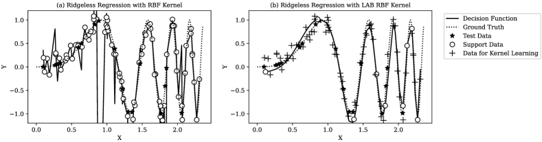
Figure 1: A toy example illustrating kernel ridgeless regression applied to a one-dimensional signal $y=\sin(2x^{3})$. In (a), the traditional RBF kernel is utilized, directly interpolating all data points. In (b), asymmetric kernel learning is applied, where a small subset is used as support data and the LAB RBF kernel is learnt from the remaining data.

Recognizing this problem, this paper introduces a solution by enhancing the model with an asymmetric kernel leaning technique. Specifically, we propose to utilize an asymmetric RBF kernel incorporating with locally adaptive bandwidths as follows,

$$\mathcal{K}({\bf x},{\bf x}_{i})=\exp\left\{-\|\theta_{i}\odot({\bf x}-{\bf x}_{i})\|_{2}^{2}\right\},\qquad\forall{\bf x}_{i}\in{\bf X}_{tr}.$$ (4)

We name the above kernel function as the Local-Adaptive-Bandwidth RBF (LAB RBF) kernel. The distinguishing feature of LAB RBF kernels, in comparison to conventional RBF kernels, is the assignment of distinct bandwidths to each sample ${\bf x}_{i}$ rather than utilizing a uniform bandwidth across all data points. In this approach, we discretely define the bandwidth for each training data point individually.

By incorporating asymmetric kernel learning, a new framework for kernel ridgeless regression is proposed in this paper. As illustrated in Figure 2, our approach not only learns the coefficient ${\bm{\alpha}}$, but also estimates the specific values of $\theta_{i}\in\mathbb{R}^{d},\forall i$ from the training data. The inclusion of data-dependent $\theta_{i}$ greatly enhances flexibility, thereby expanding the hypothesis space significantly, as we will explore in subsequent sections. Leveraging this expanded hypothesis space, it becomes feasible to search for an interpolation function with fewer support data, facilitating a discrete optimization of support data. As shown in Figure 1 (b), this method provides an estimator with varying bandwidths, enabling it to accurately approximate different frequency components of the signal. Furthermore, it demonstrates good generalization ability in the presence of noise, despite the absence of an explicit regularization term in our approach.

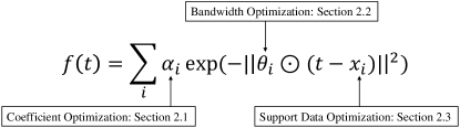
Figure 2: Optimization for evaluating $f$ in our kernel ridgeless regression framework. To enhance the model’s flexibility, we introduce trainable bandwidths, which further enable the reduce of required number of support data.

However, the absence of regularization term and the inherent asymmetry of LAB RBF kernels bring challenges to corresponding theoretical analysis. Specifically, $\theta_{i}$ and $\theta_{j}$ may differ, causing $\mathcal{K}({\bf x}_{i},{\bf x}_{j})$ to potentially differ from $\mathcal{K}({\bf x}_{j},{\bf x}_{i})$. The loss of symmetry precludes the direct application of traditional analysis tools within the scope of Reproducing Kernel Hilbert Spaces (RKHS, Cucker and Zhou (2007)), and even more general cases such as Reproducing Kernel Kreĭn Spaces (RKKS, Oglic and Gärtner (2018)) and Reproducing Kernel Banach Spaces (RKBS, Zhang et al. (2009)).

In this paper, we overcome these challenges and successfully establish the generalization analysis for the proposing algorithm that addresses kernel ridgeless regression using LAB RBF kernel learning; see Theorem 5. In particular,

1. We demonstrate a novel approach to analyze the asymmetric LAB RBF kernels within the existing framework of approximation theory (Cucker and Zhou, 2007) by introducing the integral space of Reproducing Kernel Hilbert Spaces (RKHSs). This integral space can be viewed as a non-trivial extension from the direct sum of Hilbert space, a method previously employed for analyzing Multiple Kernel Learning (MKL). To the best of our knowledge, this marks the first effort to introduce the integral space of RKHSs to machine learning.

2. We uncover the inherent sparsity of the estimator produced from LAB RBF kernels. Subsequently, we establish an equivalent $\ell_{0}$-related model within the integral space of RKHSs. This exploration addresses the origins of generalization ability and sheds light on the implicit regularization mechanisms at play.

Our key insights are twofold: (i) the trainable bandwidths effectively enrich the expansive functional spaces, enhancing the representation ability of LAB RBF kernels. This enhancement allows our algorithm to interpolate the training dataset with only a few support data. (ii) Simultaneously, the inherent sparsity of LAB RBF kernels, controlled by the number of support vectors, ensures their robust generalization ability, as evidenced in the analysis of sample error. Notably, the number of support vectors plays a pivotal role in balancing the approximation ability within the training data and the generalization ability within the test data, a observation validated by our experimental results.

The remainder of this paper is organized as follows. In Section 2, we first establish the framework of asymmetric kernel ridgeless regression. Subsequently, we incorporate LAB RBF kernels into this framework and introduce a solving algorithm for learning local bandwidths and the regression function. In Section 3, we define the function space corresponding to LAB RBF kernels, which is an integral space of RKHSs. We determine the corresponding learning model, setting the foundations for the subsequent analysis. In Section 4, we derive theoretical results on the error analysis of kernel ridgeless regression with LAB RBF kernels. In Section 5, we substantiate our theoretical findings with experimental results, demonstrating the practical implications of our proposed approach. Related works are discussed in Section 6. Finally, a conclusion is provided in Section 7.

2 Kernel Ridgeless Regression with LAB RBF Kernels

In this paper, we use calligraphic letters to denote datasets like $\mathcal{X}=\{{\bf x}_{1},\cdots,{\bf x}_{N}\}\subset\mathbb{R}^{d},\mathcal{Y}=\{y_{1},\cdots,y_{N}\}\subset\mathbb{R}$. We use captain letters in bold to denote data matrix, i.e., ${\bf X}=[{\bf x}_{1},{\bf x}_{2},\cdots,{\bf x}_{N}]\in\mathbb{R}^{M\times N},{\bf Y}=[y_{1},y_{2},\cdots,y_{N}]^{\top}\in\mathbb{R}^{N}$. We use ${\bf K}({\bf X}_{1},{\bf X}_{2})$ to denote the kernel matrix computed on datasets ${\bf X}_{1}$ and ${\bf X}_{2}$. That is, $[{\bf K}({\bf X}_{1},{\bf X}_{2})]_{ij}=\mathcal{K}({\bf x}_{i},{\bf x}_{j})$, $\forall{\bf x}_{i}\in\mathcal{X}_{1},{\bf x}_{j}\in\mathcal{X}_{2}$. The task is to find a linear function in a high dimensional feature space, denoted as $\mathbb{R}^{F}$, which models the dependencies between the features $\phi({\bf x}_{i}),\forall{\bf x}_{i}\in\mathcal{X}$ of input and response variables $y_{i},\forall y_{i}\in\mathcal{Y}$. Throughout this paper, RBF kernels are considered. In order to distinguish LAB RBF kernels from the conventional RBF kernels, we use $\theta\in\mathbb{R}^{M}_{+}$ to denote trainable bandwidths and use ${\bm{\sigma}}\in\mathbb{R}^{M}_{+}$ for fixed bandwidths.

2.1 Asymmetric Kernel Ridgeless Model: Coefficient Optimization

In this paper, we propose the utilization of LAB RBF kernels (4) in the kernel ridgeless regression model (3). However, determining the solution of the kernel ridgeless regression model with asymmetric kernels remains unresolved, as the conventional kernel trick is no longer applicable. In this section, we derive the solution using the asymmetric kernel trick, beginning with a brief review of kernel ridge regression.

Kernel ridge regression (Vovk, 2013) is one of the most elementary kernelized algorithms. The task is to find a linear function in a high dimensional feature space, denoted as $\mathbb{R}^{F}$, which models the dependencies between the features $\phi({\bf x}_{i}),\forall{\bf x}_{i}\in\mathcal{X}$ of input and response variables $y_{i},\forall y_{i}\in\mathcal{Y}$. Here, $\phi:\mathbb{R}^{M}\to\mathbb{R}^{F}$ denotes the feature mapping from the data space to the feature space. Define $\phi({\bf X})=[\phi({\bf x}_{1}),\phi({\bf x}_{2}),\cdots,\phi({\bf x}_{N})]$, then the classical optimization model is as follow:

$$\min_{{\bf w}}\;\;\frac{\lambda}{2}{\bf w}^{\top}{\bf w}+\frac{1}{2}\|{\bf Y}-\phi({\bf X})^{\top}{\bf w}\|_{2}^{2},$$ (5)

where $\lambda>0$ is a trade-off hyper-parameter. By utilizing the following well-known matrix inversion lemma (see Petersen and Pedersen (2008) for more information),

$$({\bf A}+{\bf B}{\bf D}^{-1}{\bf C})^{-1}{\bf B}{\bf D}^{-1}={\bf A}^{-1}{\bf B}({\bf C}{\bf A}^{-1}{\bf B}+{\bf D})^{-1},$$ (6)

one can obtain the solution of KRR as follow

$${\bf w}^{*} =(\phi({\bf X})\phi({\bf X})^{\top}+\lambda{\bf I}_{F})^{-1}\phi({\bf X}){\bf Y}\overset{(a)}{=}\phi({\bf X})(\lambda{\bf I}_{N}+\phi({\bf X})^{\top}\phi({\bf X}))^{-1}{\bf Y},$$

where (6) is applied in (a) with ${\bf A}=\lambda{\bf I}_{F},\;{\bf B}=\phi({\bf X}),\;{\bf C}=\phi^{\top}({\bf X}),\;{\bf D}={\bf I}_{N}$.

Next, we consider applying asymmetric kernels in KRR framework. In recent research on asymmetric kernel-based learning, asymmetric kernels are commonly assumed to be the inner product of two distinct feature mappings (see Suykens (2016); He et al. (2023); Chen et al. (2024) for reference). That is, $\mathcal{K}({\bf t},{\bf x})=\langle\phi({\bf t}),\psi({\bf x})\rangle,\;\;\forall{\bf x},{\bf t}\in\mathbb{R}^{M}.$ Then, imitating the model (5), we can formulate the asymmetric kernel ridge regression as follows,

$$\min_{{\bf w},{\bf v}}\;\lambda{\bf w}^{\top}{\bf v}+(\phi^{\top}({\bf X}){\bf w}-{\bf Y})^{\top}(\psi^{\top}({\bf X}){\bf v}-{\bf Y})$$ (7)

$$\Longleftrightarrow \min_{{\bf w},{\bf v}}\;\lambda{\bf w}^{\top}{\bf v}+\frac{1}{2}\|\phi^{\top}({\bf X}){\bf w}-{\bf Y}\|_{2}^{2}+\frac{1}{2}\|\psi^{\top}({\bf X}){\bf v}-{\bf Y}\|_{2}^{2}-\frac{1}{2}\|\psi^{\top}({\bf X}){\bf v}-\phi^{\top}({\bf X}){\bf w}\|_{2}^{2}.$$

Here, $\lambda>0$ serves as a trade-off hyper-parameter between the regularization term ${\bf w}^{\top}{\bf v}$ and the error term $(\phi^{\top}({\bf X}){\bf w}-{\bf Y})^{\top}(\psi^{\top}({\bf X}){\bf v}-{\bf Y})$. Given the existence of two feature mappings, we have two regressors in $\mathbb{R}^{F}$: $f_{1}({\bf t})=\phi^{\top}({\bf t}){\bf w}$ and $f_{2}({\bf t})=\psi^{\top}({\bf t}){\bf v}$. To enhance clarity regarding the meaning of the error term, we decompose it into the sum of three terms, as shown in the second line. The terms $\frac{1}{2}\|\phi^{\top}({\bf X}){\bf w}-{\bf Y}\|_{2}^{2}+\frac{1}{2}\|\psi^{\top}({\bf X}){\bf v}-{\bf Y}\|_{2}^{2}$ are employed to minimize the regression error. Additionally, the term $\lambda{\bf w}^{\top}{\bf v}-\frac{1}{2}\|\psi^{\top}({\bf X}){\bf v}-\phi^{\top}({\bf X}){\bf w}\|_{2}^{2}$ aims to emphasize the substantial distinction between the two regressors.

As a bilinear optimization problem, the one presented in Equation (7) is non-convex. Therefore, our attention shifts to its stationary points, leading to the following result.

Theorem 1

One of the stationary points of (7) is

$${\bf w}^{*}=\psi({\bf X})(\phi^{\top}({\bf X})\psi({\bf X})+\lambda{\bf I}_{N})^{-1}{\bf Y},\qquad\qquad{\bf v}^{*}=\phi({\bf X})(\psi^{\top}({\bf X})\phi({\bf X})+\lambda{\bf I}_{N})^{-1}{\bf Y}.$$ (8)

The proof is presented in Appendix A. Theorem 1 establishes a crucial result, demonstrating that the stationary points can still be represented as a linear combination of function evaluations on the training dataset. This validates the practical feasibility of the proposed framework. Theorem 1 indicates the proposed asymmetric KRR framework includes the symmetric one. That is, model (7) and (5) share the same stationary points when the two feature mappings are equivalent, as shown in the following corollary.

Corollary 2

If the two feature mappings $\phi$ and $\psi$ are equivalent, i.e. $\phi({\bf x})=\psi({\bf x}),\forall{\bf x}\in\mathbb{R}^{M}$, then stationary conditions of the asymmetric KRR model (7) and the symmetric KRR model (5) are equivalent. And the stationary point is ${\bf w}^{*}={\bf v}^{*}=\phi({\bf X})(\lambda{\bf I}_{N}+\phi({\bf X})^{\top}\phi({\bf X}))^{-1}{\bf Y}.$

With the conclusion in Theorem 1, we can easily apply asymmetric kernel trick $\mathcal{K}({\bf t},{\bf x})=\langle\phi({\bf t}),\psi({\bf x})\rangle$ and obtain two regression functions. By denoting a kernel matrix $[{\bf K}({\bf X},{\bf X})]_{ij}=\mathcal{K}({\bf x}_{i},{\bf x}_{j})=\langle\phi({\bf x}_{i}),\psi({\bf x}_{j})\rangle$, $\forall{\bf x}_{i},{\bf x}_{j}\in\mathcal{X}$, we have:

$$f_{1}({\bf t})=\phi({\bf t})^{\top}{\bf w}^{*}={\bf K}({\bf t},{\bf X})({\bf K}({\bf X},{\bf X})+\lambda{\bf I}_{N})^{-1}{\bf Y},$$ (9)

$$f_{2}({\bf t})=\psi({\bf t})^{\top}{\bf v}^{*}={\bf K}^{\top}({\bf X},{\bf t})({\bf K}^{\top}({\bf X},{\bf X})+\lambda{\bf I}_{N})^{-1}{\bf Y}.$$

The scenario of obtaining two regressors does not occur in a symmetric setting and the existance of the second regressor is often overlooked in prior works on asymmetric kernel regression. Consequently, the relationship between these regressors remains unclear. We discuss this question in Appendix B from a primal-dual perspective. Our analysis reveals that the approximation error of these two regressors can be computed analytically. Notably, if ${\bf K}({\bf X},{\bf X})$ is asymmetric, the errors generally differ, leading to a significant observation: the two regressors represent distinct functions converging toward the ground truth from divergent directions.

When LAB RBF kernels are utilized, the computation of ${\bf K}({\bf X},{\bf t})$ necessitates a bandwidth that is dependent on the testing data ${\bf t}$. Given the impracticality of estimating bandwidths for testing data, we restrict our computations to ${\bf K}({\bf t},{\bf X})$. As a result, only $f_{1}$ in Equation (9) is applicable for our algorithm. From Mercer’s theorem we know that for traditional RBF kernels, there exists a feature mapping function $\phi(\cdot):\mathcal{X}\to\mathcal{F}$ satisfying that $\mathcal{K}_{\sigma}({\bf t},{\bf x})=\langle\phi_{\sigma}({\bf t}),\phi_{\sigma}({\bf x})\rangle$. Recall the definition of the proposed LAB RBF kernel function over dataset $\mathcal{X}$ in Equation (4), we can define

$$\phi({\bf t})=[\phi^{\top}_{\theta_{1}}({\bf t})\;\;\phi^{\top}_{\theta_{2}}({\bf t})\;\;\cdots\;\;\phi^{\top}_{\theta_{N}}({\bf t})]^{\top},$$

$$\psi({\bf x})=[\phi^{\top}_{\theta_{1}}({\bf x})\delta({\bf x}-{\bf x}_{1})\;\;\phi^{\top}_{\theta_{2}}({\bf x})\delta({\bf x}-{\bf x}_{2})\;\;\cdots\;\;\phi^{\top}_{\theta_{N}}({\bf x})\delta({\bf x}-{\bf x}_{N})]^{\top},$$

where $\theta_{i}$ is the corresponding bandwidth for data ${\bf x}_{i}$ and $\delta(\cdot)$ denotes the Dirac delta function. Then we can decompose the asymmetric LAB RBF kernels defined over a dataset $\mathcal{X}$ as the inner product of $\phi$ and $\psi$. That is, given dataset $\mathcal{X}$ and corresponding bandwidth set ${\bm{\Theta}}=\{\theta_{1},\cdots,\theta_{N}\}$, the LAB RBF kernel defined over $\mathcal{X}$ and ${\bm{\Theta}}$ satisfies

$$\mathcal{K}_{\bm{\Theta}}({\bf t},{\bf x}_{i})=\exp\{-\|\theta_{i}\odot({\bf t}-{\bf x}_{i})\|^{2})\}=\langle\phi({\bf t}),\psi({\bf x}_{i})\rangle,\qquad\forall{\bf t}\in\mathbb{R}^{d},{\bf x}_{i}\in\mathcal{X}.$$ (10)

Finally, substituting Equation (10) into $f_{1}$, we obtain the solution of kernel ridgeless regression model with LAB RBF kernels by setting regularization coefficient $\lambda$ in (9) equals to zero:

$$f_{\mathcal{Z},{\bm{\Theta}}}({\bf t}) \triangleq\phi({\bf t})^{\top}{\bf w}=\phi({\bf t})^{\top}\psi({\bf X}){\bm{\alpha}}=\sum_{i=1}^{N}\alpha_{i}\exp\left\{-\|\theta_{i}\odot({\bf t}-{\bf x}_{i})\|_{2}^{2}\right\},$$ (11)

$${\bm{\alpha}} =\lim_{\lambda\rightarrow 0}\left\{({\bf K}_{\bm{\Theta}}({\bf X},{\bf X})+\lambda{\bf I}_{N})^{-1}{\bf Y}\right\},$$

where $\mathcal{Z}\triangleq\{\mathcal{X},\mathcal{Y}\}$ and $[{\bf K}_{\bm{\Theta}}({\bf X},{\bf X})]_{ij}\triangleq\exp\left\{-\|\theta_{j}\odot({\bf x}_{i}-{\bf x}_{j})\|_{2}^{2}\right\},\forall{\bf x}_{i},{\bf x}_{j}\in\mathcal{X}$.

2.2 LAB RBF Kernel Learning: Bandwidth Optimization

The solutions presented in (11) represent simple interpolation functions that may be susceptible to noise in the data. To enhance generalization ability, we employ kernel learning techniques to augment model flexibility and subsequently reduce model complexity. It is essential to note that the solution in (11) corresponds to a stationary point, necessitating additional data for optimizing the bandwidths ${\bm{\Theta}}$. Our algorithm thus divides the available data into two parts: (i) a subset of the available data serves as support data, used for constructing the regression function according to Equation (11), and (ii) the remaining data, termed training data, is utilized for the optimization of bandwidths.

Assume a support dataset $\mathcal{Z}_{sv}=\{\mathcal{X}_{sv},\mathcal{Y}_{sv}\}$ and a training dataset $\mathcal{Z}_{tr}=\{\mathcal{X}_{tr},\mathcal{Y}_{tr}\}$ are pre-given, then according to Equation (11), the optimization model for bandwidths ${\bm{\Theta}}$ is,

$${\bm{\Theta}}^{*} =\arg\min_{{\bm{\Theta}}}\sum_{\{{\bf x}_{i},y_{i}\}\in\mathcal{Z}_{tr}}\left(y_{i}-f_{\mathcal{Z}_{sv},{\bm{\Theta}}}({\bf x}_{i})\right)^{2}$$ (12)

$$=\arg\min_{{\bm{\Theta}}}\sum_{\{{\bf x}_{i},y_{i}\}\in\mathcal{Z}_{tr}}\left(y_{i}-{\bf K}_{\bm{\Theta}}({\bf x}_{i},{\bf X}_{sv}){\bf K}^{-1}_{\bm{\Theta}}({\bf X}_{sv},{\bf X}_{sv}){\bf Y}_{sv}\right)^{2}.$$

Being a function that interpolates a small dataset without any regularization, it is apparent that the generalization performance of $f_{\mathcal{Z}_{sv},{\bm{\Theta}}}$ in Equation 11 does not meet expectations. Nevertheless, through the training of bandwidths ${\bm{\Theta}}$ with additional data, we can significantly enhance the generalization capacity of $f_{\mathcal{Z}_{sv},{\bm{\Theta}}}$.

2.3 Dynamic Strategy: Support Data Optimization

While in kernel methods we can always achieve perfect interpolation of training data when all data points are used as support data, the resulting interpolation function often lacks robust generalization ability. In our approach, integrating asymmetric kernel learning techniques, i.e., the optimization in (12), enables us to achieve a good fit with fewer support data points. Drawing from traditional regularization scenarios, we aim to minimize the support data while effectively approximating the training data. However, this strategy introduces a discrete optimization problem, posing challenges for accurate solution finding.

$$\mathcal{Z}_{sv}=\min_{\mathcal{Z}\subset\mathcal{Z}_{tr}} |\mathcal{Z}|$$ (13)

$$\mathrm{s.t.} y_{i}=f_{\mathcal{Z},{\bm{\Theta}}}({\bf x}_{i}),\quad\forall\{{\bf x}_{i},y_{i}\}\in\mathcal{Z}_{tr},$$

where $|\mathcal{Z}|$ denotes the cardinality of set $\mathcal{Z}$, i.e. the number of data in $\mathcal{Z}$.

Though this discrete optimization presents challenges for direct optimization, numerous existing strategies for data selection can be employed. For instance, it resembles the selection of centers in Nyström approximation (see Williams and Seeger (2000); Rudi et al. (2017) for details). Consequently, the subset selection strategies utilized in these existing works are applicable to the proposed algorithm. Additional experiments evaluating the performance of the proposed algorithm with various reasonable strategies are elaborated in Appendix G.

In this paper, to facilitate theoretical analysis, we apply a dynamic strategy for selecting support data. Initially, we uniformly select $N_{0}$ support data points according to their labels, and then: (i) Optimize (12) to obtain $f_{\mathcal{Z}_{sv},{\bm{\Theta}}}$. (ii) Compute approximation error $e_{i}=(f_{\mathcal{Z}_{sv},{\bm{\Theta}}}({\bf x}_{i})-y_{i})^{2},\forall\{{\bf x}_{i},y_{i}\}\in\mathcal{Z}_{tr}$. (iii) Add data with first $k$ largest error to support dataset. Repeat the above process until all approximation error is less than a pre-given threshold $B$. The overall algorithm is presented in Algorithm 1.

By dynamic strategy, we actually obtain an important property of the resulting estimator, i.e.,

$$(f_{\mathcal{Z}_{sv},{\bm{\Theta}}}({\bf x}_{i})-y_{i})^{2}\leq B,\qquad\forall\{{\bf x}_{i},y_{i}\}\in\mathcal{Z}_{sv}\cup\mathcal{Z}_{tr},$$ (14)

which essentially stands the accuracy of the interpolation of $f_{\mathcal{Z}_{sv},{\bm{\Theta}}}$ on the training dataset. And in the next section, we will shown it helps when analyzing the approximation behavior of LAB RBF kernels.

1:Input: Data $\mathcal{Z}=\{\mathcal{X},\mathcal{Y}\}$.

2:Initialization: Error tolerance $B>0$, initial bandwidth ${\bm{\Theta}}^{(0)}>0$, learning rate for gradient descent method $\eta>0$, $k$ for the dynamic strategy, and uniformly sampled support dataset $\mathcal{Z}_{sv}^{(0)}=\{\mathcal{X}_{sv}^{(0)},\mathcal{Y}_{sv}^{(0)}\}\subset\mathcal{Z}$.

3:t=0.

4:repeat

5:     $\tilde{{\bm{\Theta}}}^{(0)}={\bm{\Theta}}^{(t)}$.

6:     for $l=1,\cdots,L$ do $\triangleright$ Optimize ${\bm{\Theta}}$ via SGD

7:         Randomly sample a subset $\{\mathcal{X}_{s},\mathcal{Y}_{s}\}\subset\mathcal{Z}\setminus\mathcal{Z}_{sv}$.

8:         Compute $\tilde{{\bm{\Theta}}}^{(l)}=\tilde{{\bm{\Theta}}}^{(l-1)}-\eta\frac{\partial}{\partial{\bm{\Theta}}}\|f_{\mathcal{Z}_{sv}^{(t)},\tilde{{\bm{\Theta}}}^{(l)}}({\bf X}_{s})-{\bf Y}_{s}\|^{2}$ according to (12).

9:     end for

10:     ${\bm{\Theta}}^{(t+1)}=\tilde{{\bm{\Theta}}}^{(L)}$.

11:     Compute error $e_{i}=(f_{\mathcal{Z}_{sv}^{(t)},{\bm{\Theta}}^{(t)}}({\bf x}_{i})-y_{i})^{2}$ for all data $\{{\bf x}_{i},y_{i}\}\in\mathcal{Z}\setminus\mathcal{Z}_{sv}$.

12:     if $\max_{i}e_{i}\leq B$ then $\triangleright$ Dynamically adding support data

13:         break.

14:     else

15:         Select the first $k$ samples with the highest errors and include them in the support dataset, resulting in $\mathcal{Z}_{sv}^{(t+1)}$.

16:     end if

17:     t=t+1.

18:until the maximal number of iteration is exceeded.

19:Compute the ${\bm{\alpha}}={\bf K}^{-1}_{{\bm{\Theta}}^{(t)}}({\bf X}^{(t)}_{sv},{\bf X}_{sv}^{(t)}){\bf Y}_{sv}^{(t)}$. $\triangleright$ Compute the final function

20:Return ${\bm{\alpha}},\mathcal{Z}^{(t)}_{sv}$ and ${\bm{\Theta}}^{(t)}$.

Algorithm 1 Learning LAB RBF kernels with SGD and dynamic strategy.

3 Theoretical Interpretation

3.1 Enlarged hypothesis space: Integral Space of RKHSs

To comprehend the learning dynamics of Algorithm 1 and LAB RBF kernels, it is imperative to clarify the underlying function spaces. The LAB RBF kernel, defined in Equation (4), employs distinct bandwidths for individual samples, thus associating itself with multiple RKHSs. Unlike Multiple Kernel Learning (MKL, Gönen and Alpaydın (2011)), which explores a search space comprised of a finite number of RKHSs with a discrete domain of bandwidths (i.e., the kernel dictionary, as discussed in Suzuki (2011)), LAB RBF kernels exhibit a continuous feasible domain of bandwidths. This characteristic results in a function space that surpasses a direct sum of RKHSs. To enhance the understanding of LAB RBF kernels, this paper introduces the concept of the integral space of RKHSs as a novel hypothesis space.

Given a continuous bandwidth candidate set $\Omega\subset\mathbb{R}_{+}^{M}$, a traditional RBF kernel with a fixed uniform bandwidth ${\bm{\sigma}}\in\Omega$ has a form of $\mathcal{K}_{\bm{\sigma}}({\bf x}_{i},{\bf x}_{j})=\exp\{-\|{\bm{\sigma}}\odot({\bf x}_{i}-{\bf x}_{j})\|_{2}^{2}\}$. The RKHS introduced by $\mathcal{K}_{\bm{\sigma}}$ is denoted as $\mathcal{H}_{\bm{\sigma}}$. That is, $\forall{\bf x}\in\mathcal{X}$, $\mathcal{K}_{\bm{\sigma}}(\cdot,{\bf x})\in\mathcal{H}_{\bm{\sigma}}$ and we use $f_{\bm{\sigma}}$ to denote functions belonging to $\mathcal{H}_{\bm{\sigma}}$. Then the integral space of RKHSs defined over $\Omega$ takes the following form,

$$\mathcal{H}_{\Omega} =\int_{{\bm{\sigma}}\in\Omega}\mathcal{H}_{\bm{\sigma}}d\mu({\bm{\sigma}})=\left\{f=(f_{\bm{\sigma}})_{{\bm{\sigma}}\in\Omega}:\left.\int_{{\bm{\sigma}}\in\Omega}\|f_{\bm{\sigma}}\|^{2}_{\mathcal{H}_{\bm{\sigma}}}d\mu({\bm{\sigma}})<\infty\right.\right\},$$

where $(f_{\bm{\sigma}})_{{\bm{\sigma}}\in\Omega}$ is a measurable cross-section and $\mu({\bm{\sigma}})$ denotes a probability distribution of ${\bm{\sigma}}$. For more theoretical discussion of integral spaces of RKHSs, one can refer to Wils (1970); Hotz and Fabian (2012). It has been proved that $\mathcal{H}_{\Omega}$ is again a Hilbert space, where the inner product between $f=(f_{\bm{\sigma}})_{{\bm{\sigma}}\in\Omega},\;g=(g_{\bm{\sigma}})_{{\bm{\sigma}}\in\Omega}\in\mathcal{H}_{\Omega}$ is defined as

$$\langle f,g\rangle_{\mathcal{H}_{\Omega}}:=\int_{{\bm{\sigma}}\in\Omega}\langle f_{\bm{\sigma}},g_{\bm{\sigma}}\rangle_{\mathcal{H}_{\bm{\sigma}}}d\mu({\bm{\sigma}}).$$

Consequently, it holds that $f({\bf x})=\int_{{\bm{\sigma}}\in\Omega}f_{\bm{\sigma}}({\bf x})d\mu({\bm{\sigma}}),\forall{\bf x}\in\mathcal{X}.$ Then the corresponding norm is defined as

$$\|f\|^{2}_{\mathcal{H}_{\Omega}}:=\min\left\{\int_{{\bm{\sigma}}\in\Omega}\|f_{\bm{\sigma}}\|^{2}_{\mathcal{H}_{\bm{\sigma}}}d\mu({\bm{\sigma}}):f=(f_{\bm{\sigma}})_{{\bm{\sigma}}\in\Omega}\right\},$$

where $\|f_{\bm{\sigma}}\|^{2}_{\mathcal{H}_{\bm{\sigma}}}=\langle f_{\bm{\sigma}},f_{\bm{\sigma}}\rangle_{\mathcal{H}_{\bm{\sigma}}}$.

Recall that in Algorithm 1, ${\bm{\Theta}}$ represents a discrete set. Consequently, the estimator $f_{\mathcal{Z}_{sv},{\bm{\Theta}}}$ is constructed from a finite number of kernels, thereby situating it within a sum space of RKHSs associated with these kernels. It is important to note that this inference relies on the assumption of a fixed ${\bm{\Theta}}$. When optimizing ${\bm{\Theta}}$, this sum space also changes according to the variations in bandwidths, as shown in Figure 4. Mathematically, we assume a sum space of RKHSs generated from a bandwidth set ${\bm{\Theta}}$ is denoted as $\mathcal{H}_{\bm{\Theta}}$. Recall that in our approach, a continuous feasible domain of bandwidth is considered, i.e., ${\bm{\Theta}}\subset\Omega$. Consequently, the hypothesis space involved in our approach is the union of all possible $\mathcal{H}_{\bm{\Theta}}$, i.e.

$$\mathrm{Hypothesis\;Space:}\bigcup_{{\bm{\Theta}}\subset\Omega}\mathcal{H}_{\bm{\Theta}}=\mathcal{H}_{\Omega},$$

which indicates that the hypothesis space remains an integral space rather than a fixed sum space.

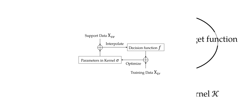
Figure 3: Optimal subspace selection when learning kernels.

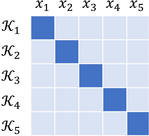
Figure 4: Coefficient matrix of $f_{\mathcal{Z},{\bm{\Theta}}}$, exhibiting sparse property.

3.2 Sparsity of the Estimator

With the established hypothesis space $\mathcal{H}_{\Omega}$, this section delineates the sparse property of the estimator generated by LAB RBF kernels. This characterization aids in our deeper comprehension of the generalization ability of the proposed model. In Algorithm 1, two levels of sparsity are observed:

• Reduced support data: The number of support data points is significantly lower than the total number of training data points. While this sparsity is artificially determined algorithmically, its essential reason lies in the sufficiently large hypothesis space. This expansive hypothesis space enables us to employ fewer support data points to effectively approximate the entire training dataset. This sparsity leads to a fact that $f_{\mathcal{Z}_{sv},{\bm{\Theta}}}$ belongs to a small subspace $\mathcal{H}_{\bm{\Theta}}$ of $\mathcal{H}_{\Omega}$.

• Inherent sparsity of LAB RBF kernels: $f_{\mathcal{Z}_{sv},{\bm{\Theta}}}$ demonstrate sparsity within the hypothesis space $\mathcal{H}_{\bm{\Theta}}$, contributing to a more efficient representation of the data.

In the following, we show the latter sparsity of $f_{\mathcal{Z}_{sv},{\bm{\Theta}}}$ mathematically by comparing with general function in $\mathcal{H}_{\bm{\Theta}}$. Given dataset $\{{\bf x}_{i},y_{i}\}_{i=1}^{N}$, the hypothesis space considered here is taken to be the linear span of the set $\{\mathcal{K}_{\bm{\sigma}}(\cdot,{\bf x}_{i})\}$, $\forall i=1,\cdots,N,\;\forall{\bm{\sigma}}\in\Omega$. This space forms a subspace of $\mathcal{H}_{\Omega}$. In $f_{\mathcal{Z}_{sv},{\bm{\Theta}}}$, only bandwidths in ${\bm{\Theta}}$ are valid, therefore we constrain ${\mu}(\sigma)=\sum_{\theta_{i}\in{\bm{\Theta}}}\delta(\sigma-\theta_{i})$. Then function in this hypothesis space takes a formulation as $f(\cdot)=\sum_{\sigma\in\Theta}f_{\sigma}(\cdot)=\sum_{\sigma\in\Theta}\sum_{i=1}^{N_{sv}}\alpha_{\sigma,i}\mathcal{K}_{\sigma}(\cdot,{\bf x}_{i}),$ where the coefficients ${\bm{\alpha}}_{\bm{\sigma}}\in\mathbb{R}^{{N_{sv}}}$.

Let $\|{\bm{\alpha}}\|_{0}=\sum_{i=1}^{N}\mathbb{I}(\alpha_{i}\neq 0)$, where $\mathbb{I}$ is a indicator function. We can define a $\ell_{0}$-related sparse regularization penalty as below,

$$\mathcal{R}_{0}(f) :=\min\left\{\int_{{\bm{\sigma}}\in\Omega}\|{\bm{\alpha}}_{\bm{\sigma}}\|_{0}d\mu({\bm{\sigma}}):f=(f_{\bm{\sigma}})_{{\bm{\sigma}}\in\Omega},f_{\bm{\sigma}}(\cdot)=\sum_{i=1}^{N}\alpha_{{\bm{\sigma}},i}\mathcal{K}_{\bm{\sigma}}(\cdot,{\bf x}_{i})\right\}.$$ (15)

Without sparsity, a general function in $\mathcal{H}_{\bm{\Theta}}$ typically results in $\mathcal{R}_{0}(f)$ being approximately equal to $|\Theta|\times{N_{sv}}$. However, recall the function estimated by LAB RBF kernels in (11), generated from the same kernels and data, takes a formulation like:

$$f_{\mathcal{Z}_{sv},{\bm{\Theta}}}(\cdot)=\sum_{i=1}^{N_{sv}}\hat{\alpha}_{i}\mathcal{K}_{\theta_{i}}(\cdot,x_{i})=\sum_{\sigma\in\Theta}\sum_{i=1}^{N_{sv}}\alpha_{\sigma,i}\mathcal{K}_{\sigma}(\cdot,x_{i}).$$

Comparing their coefficients, we say $f_{\mathcal{Z}_{sv},{\bm{\Theta}}}$ exhibits sparsity because

$$\alpha_{\sigma,i}=\begin{cases}\hat{\alpha}_{i},\;&\mathrm{if}\;\sigma=\theta_{i},\\ 0,\;&\mathrm{otherwise}.\end{cases}$$

This sparsity can be quantified by the measurement $\mathcal{R}_{0}(f_{\mathcal{Z}{sv},{\bm{\Theta}}})=N_{sv}$, or visually depicted in Figure 4. In this regard, $f_{\mathcal{Z}_{sv},{\bm{\Theta}}}$ demonstrates enhanced sparsity compared to a typical function within the sum space $\mathcal{H}_{\Theta}$, not to mention functions within the integral space $\mathcal{H}_{\Omega}$.

3.3 Equivalence to a $\ell_{0}$-related Model

Utilizing this sparse property, we can gain deeper insights into $f_{\mathcal{Z}_{sv},{\bm{\Theta}}}$ by formulating a sparse optimization model, leveraging the $\mathcal{R}_{0}$ regularization term. Let us define the empirical error $\mathcal{E}_{z}(f)$ and the generalization error $\mathcal{E}_{\rho}(f)$ as follows,

$$\mathcal{E}_{\bf z}(f)=\frac{1}{N}\sum_{{{\bf x}_{i},y_{i}}\in\mathcal{Z}_{tr}}(f({\bf x}_{i})-y_{i})^{2},\quad\quad\quad\mathcal{E}_{\rho}(f)=\int_{\mathcal{Z}}(f({\bf x})-y)^{2}d\rho.$$

Then we have

$$f_{{\bf z},\lambda}=\arg\min_{\begin{subarray}{c}f\in\mathcal{H}_{\Omega}\\ \{{\bm{\theta}}_{i}\}\subset\Omega\end{subarray}}\mathcal{E}_{\bf z}(f)+\lambda\mathcal{R}_{0}(f)$$ (16)

$$\;\;\;\mathrm{s.t.}\quad{\mu}({\bm{\sigma}})=\sum_{i=1}^{N_{sv}}\delta({\bm{\sigma}}-\theta_{i}),$$

where $\lambda,N_{sv}>0$ are pre-given parameters, and $\delta(\cdot)$ denotes the Dirac delta function.

Optimizations involving $\ell_{0}$ norm are generally challenging to solve directly as they often give rise to an NP-hard discrete optimization (Natarajan, 1995), and the problem in (16) is no exception. However, as demonstrated by the following proposition, Algorithm 1 for learning LAB RBF kernel yields an estimator that closely approximates the optimal solution of (16).

Proposition 3

Let $f_{\mathcal{Z}_{sv},{\bm{\Theta}}}$ denotes the regressor produced by Algorithm 1 with dynamics strategy (i.e., $f_{\mathcal{Z}_{sv},{\bm{\Theta}}}$ satisfies (14)) on dataset $\mathcal{Z}=\{{\bf x}_{i},y_{i}\}_{i=1}^{N}$. Then there exists a $\lambda>0$ such that the optimal solution $f_{{\bf z},\lambda}$ of (16) satisfies that $\mathcal{R}_{0}(f_{\mathcal{Z}_{sv},{\bm{\Theta}}})=\mathcal{R}_{0}({f}_{{\bf z},\lambda})$, and $0<\mathcal{E}_{\bf z}(f_{\mathcal{Z}_{sv},{\bm{\Theta}}})-\mathcal{E}_{\bf z}({f}_{{\bf z},\lambda})\leq B.$

The proof is presented in Appendix D. This proposition shows that $f_{\mathcal{Z}_{sv},{\bm{\Theta}}}$ is a $B$-optimal solution of model (16) with some $\lambda$. It establishes a link between a well-trained function derived by kernel ridgeless regression with a LAB RBF kernel — exhibiting good interpolation performance on the training dataset — and the optimal solution of an $\ell_{0}$-related model within the integral space of RKHSs. This relationship effectively highlights the superiority of our method’s strategy for enhancing model flexibility through the learning of the LAB kernel function. Specifically,

• The model’s enhanced flexibility is primarily achieved through the expansion of the hypothesis space, where the estimator is optimized from an integral space of RKHSs $\mathcal{H}_{\Omega}$. This expansion is enabled by optimizing ${{\bm{\theta}}_{i}}$, which selects the optimal subspace from $\mathcal{H}_{\Omega}$, as illustrated in Figure 4. Consequently, the algorithm efficiently minimizes the distance to the underlying function, leading to a small bias.

• The large capacity of hypothesis space also raises the probability of interpolating training data with fewer support data, evidenced by the sparse coefficients of $f_{\mathcal{Z}_{sv},{\bm{\Theta}}}$. This sparsity characteristic clarifies the origin of the model’s generalization capability: with an implicit $\ell_{0}$-related term in effect, controlled by the number of support data, our algorithm effectively reduces variance.

It is worth noting that, despite the absence of a regularization term in the kernel ridgeless regression framework, our approach effectively maintains a balance between bias and variance through our dynamic strategy. From model (16) and Proposition 3, it is determined that a smaller number of support data implies a stronger regularization effect. Note that kernel machines can always interpolate all training data; that is, the value of $B$ can be arbitrarily close to 0 as the number of support data increases. Therefore, our proposed dynamic strategy proves effective as it seeks a balance between the number of support data and the empirical approximation error. The hyper-parameter $B$, which varies with datasets, essentially serves as a trade-off parameter between bias and variance, resembling most regularization schemes.

4 Approximation Analysis

In the preceding sections, we introduced our kernel learning algorithm and corresponding theoretical explanation. The extensive capacity of the integral space of RKHSs and the utilization of the $\ell_{0}$ norm contribute to the exceptional performance of LAB RBF kernels, as evidenced by the experiments in Section 5. Nevertheless, these characteristics also pose significant challenges for approximation analysis. To derive the learning rate of ${f}_{{\bf z},\lambda}$, this section employs three key techniques:

• Addressing the discrete nature of the $\ell_{0}$ norm, we use the optimal estimator of a $\ell_{q}\;(0<q<1)$-regularized model as a stepping-stone function.

• The Rademacher chaos complexity is employed to establish the upper bound of the sample error in the integral space of RKHSs, leveraging the properties of the optimal solution ${f}_{{\bf z},\lambda}$.

• A refined iteration technique is applied to obtain an accurate upper bound of $\mathcal{R}_{0}({f}_{{\bf z},\lambda})$.

The main result is presented in Theorem 5.

4.1 Assumptions and Main Result

We prepare some notations and assumptions for the following analysis. Let $\rho$ be a Borel probability distribution on $\mathcal{Z}$. Then from Proposition 1.8 in Cucker and Zhou (2007), the target regression function can be expressed as $f_{\rho}=\int_{\mathcal{Y}}yd\rho(y|{\bf x}),\;{\bf x}\in\mathcal{X},$ where $\rho(\cdot|{\bf x})$ is the conditional probability measure induced by $\rho$ at ${\bf x}$. Thoughout this paper, we assume that $f_{\rho}$ belongs to a Sobelve space $\mathcal{H}^{s}(\mathbb{R}^{d})$ with some $s>0$, and $\rho(\cdot|{\bf x})$ is support on $[-M,M]$. That is,

Assumption 1

For some constant $1\leq M<\infty$, there hold $|f_{\rho}({\bf x})|\leq M$ and $|y|\leq M$.

Such uniformly boundedness assumptions of the output has been widely used in learning theory e.g., Zhou (2003); Wu et al. (2006); Smale and Zhou (2007). And it also indicates a bounded noise level that $|y-f_{\rho}({\bf x})|\leq 2M$. Based on this assumption, we can apply the following projection operator to our analysis for better estimates.

Definition 4

For $M>0$, the projection operator $\pi_{M}$ is defined as

$$\pi_{M}(t)=\begin{cases}-M&\mathrm{if\;}t\leq-M,\\ t&\mathrm{if\;}-M<t\leq M,\\ M&\mathrm{if\;}t>M.\\ \end{cases}$$

The projection of a function $f:X\to\mathbb{R}$ is defined by $\pi_{M}(f)({\bf x})=\pi_{M}(f({\bf x})),\forall{\bf x}\in\mathcal{X}.$

Such projection operator is introduced in Chen et al. (2004) and is helpful in estimating the $\|\cdot\|_{\infty}$ bound in the following analysis. Under Assumption 1, it is natural to project the estimator $f$ into the same interval as $f_{\rho}$. Thus, we shall consider the error $\|\pi_{M}(f)-f_{\rho}\|_{\mathcal{L}^{2}_{\rho_{\bf X}}}$.

In the previous section, we point out that LAB RBF kernels are actually thed combination of RBF kernels with trainable bandwidths belonging to a pre-given closed interval $\Omega$. Theoretical properties of RBF kernels have been well investigated before. One can refer to Ye and Zhou (2008); Eberts and Steinwart (2011) for RBF kernels with fixed bandwidths, and Ying and Zhou (2007) for RBF kernels with flexible bandwidths. Consider $\mathcal{K}_{\sigma}({\bf x},{\bf x}^{\prime})=\exp\{-\sigma\|{\bf x}-{\bf x}^{\prime}\|^{2}_{2}\},\forall\sigma\in\Omega.$ It has been proved that $\mathcal{K}_{\sigma}\in\mathcal{C}^{\infty}(\mathcal{X}\times\mathcal{X})$ and there exists a bound $\|\mathcal{K}_{\sigma}\|_{C^{\infty}(\mathcal{X}\times\mathcal{X})}<\infty,\;\;\forall\sigma\in\Omega.$ Therefore we can define

$$\kappa:=\sup_{\sigma\in\Omega}\|\mathcal{K}_{\sigma}\|_{C^{\infty}(\mathcal{X}\times\mathcal{X})}<\infty.$$

Given a continuous kernel $\mathcal{K}_{\sigma}$, it can define an integral operator on $\mathcal{L}_{\rho_{\bf X}}^{2}(\mathcal{X})$ as follows

$$\mathcal{L}_{\mathcal{K}}f({\bf x})=\int_{\mathcal{X}}\mathcal{K}_{\sigma^{*}}({\bf x},{\bf t})f({\bf t})d\rho_{\bf X}({\bf t}),\quad{\bf x}\in\mathcal{X},\quad\forall f\in\mathcal{L}_{\rho_{\bf X}}^{2}(\mathcal{X}).$$ (17)

And a Mercer kernel can be defined as $\tilde{\mathcal{K}}_{\sigma}({\bf t},{\bf x})=\int_{\mathcal{X}}\mathcal{K}_{\sigma}({\bf t},{\bf u})\mathcal{K}_{\sigma}({\bf x},{\bf u})d\rho_{\bf X}({\bf u}).$ In this paper, we use the RKHS $\mathcal{H}_{\tilde{K}_{\sigma}}$ satisfying $\sigma\in\Omega$ to approximate $f_{\rho}$. Following the definition in Ying and Zhou (2007), the regularization error associated with a flexible $\mathcal{H}_{\tilde{K}_{\sigma}}$ is defined as follows,

$$\mathcal{D}(\gamma)=\inf_{\sigma\in\Omega}\inf_{f\in\mathcal{H}_{\tilde{K}_{\sigma}}}\left\{\mathcal{E}_{\rho}(f)-\mathcal{E}_{\rho}(f_{\rho})+\gamma\|f\|_{\mathcal{H}_{\tilde{K}_{\sigma}}}\right\}.$$ (18)

As $\gamma\rightarrow 0$, the decay rate of $\mathcal{D}(\gamma)$ measures the lower bound of the approximation ability of the hypothesis space, which in the literature of learning theory are generally assumed as follows (e.g., Cucker and Zhou (2007); Steinwart and Christmann (2008)).

Assumption 2

For some constant $0<\beta\leq 1$ and $c_{\beta}\geq 1$, it holds

$$\mathcal{D}(\gamma)\leq c_{\beta}\gamma^{\beta},\;\;\forall\gamma>0.$$

Then we present the main result.

Theorem 5

Assume the regression $f_{\rho}\in\mathcal{H}^{s}(\mathcal{X})$ with some $s>0$. Given $\Omega$, suppose Assumption 1 and Assumption 2 hold with $M\in[1,+\infty)$ and $\beta\in(0,1]$. If $\xi\in(0,\frac{\beta}{4})$ (which can be arbitrarily small), $\lambda=(\frac{\xi}{\kappa^{2}})^{\frac{1-\xi}{1+\xi}}N^{-\tilde{\tau}}$ with $\tilde{\tau}=\beta/2(1+\xi)(\xi+\beta-\xi\beta)$ and $\delta\in(0,1)$, then with at least $1-\delta$ confidence, it holds that

$$\|\pi_{M}(f_{{\bf z},\lambda}) -f_{\rho}\|_{L_{\rho_{\bf X}}}\leq\tilde{C_{3}}\log^{2}\left(\frac{36}{\delta}\right)\left(\log\left(\frac{72}{\delta}\right)+\log(J(d,s,\beta,\xi)+1)\right)^{2J(d,s,\beta,\xi)}N^{-(\frac{\beta}{4}-\xi)},$$

and

$$\mathcal{R}_{0}(f_{{\bf z},\lambda})\leq C_{3}(\log J(d,s,\beta,\xi))^{3}\left(\log\left(\frac{24}{\delta}\right)+\log(J(d,s,\beta,\xi)+1)\right)^{2J(d,s,\beta,\xi)}N^{\tilde{\tau}+\xi-\frac{\beta}{4}},$$

where $C_{3}$ and $\tilde{C_{3}}$ are some positive constant independent of $N$ and $\delta$ and $J(d,s,\beta,\xi)$ is defined as

$$J(d,s,\beta,\xi)=\max\left\{\frac{\log\frac{2s\beta+2s\xi(1-\beta)-2d\beta}{6s\beta+8s\xi(1-\beta)-d\beta}}{\log\frac{d+2s}{2d}},\frac{\beta}{(1-\beta)\xi^{2}+\xi}\right\}.$$

The convergence rate of Algorithm (16) concerning the accuracy, as well as the model complexity, with respect to the data number is provided by Theorem 5. This pioneering analysis in the integral space of RKHSs unveils valuable insights. The convergence rate can be arbitrarily close to $N^{-\beta/4}$. The sparsity of $f_{{\bf z},\lambda}$, determined by $\mathcal{R}_{0}(f_{{\bf z},\lambda})/N$, demonstrates a superior convergence rate compared to $O\left(N^{-\left(\frac{1}{2}+\frac{\beta}{4}-\xi\right)}\right)$, thanks to the constraint $\tilde{\tau}\leq\frac{1}{2}$. Importantly, $\mathcal{R}_{0}(f_{{\bf z},\lambda})$ also acts as an upper bound for the number of valid bandwidths, facilitating the practical selection of support data. In the literature of approximation analysis, the specific value of $\beta$ in Assumption 2 is determined by certain assumptions regarding the relationship between the underlying function $f_{\rho}$ and the hypothesis spaces. Here we suppose $f_{\rho}\in\mathcal{H}^{s}(\mathcal{X})$ for some $s>0$. According to Proposition 22 in Ying and Zhou (2007), Assumption 2 holds true. However, we refrain from introducing additional assumptions for $s$ to ascertain the specific value of $\beta$. Further details on the value of $\beta$ can be found in Ying and Zhou (2007).

4.2 Framework of Convergence Analysis

From Cucker and Zhou (2007), it holds that $\|f-f_{\rho}\|^{2}_{\mathcal{L}_{\rho_{\bf X}}}=\mathcal{E}_{\rho}(f)-\mathcal{E}_{\rho}(f_{\rho}),\forall f:\mathcal{X}\rightarrow\mathbb{R}$. Thus Theorem 5 can be obtained by estimating the upper bound of $\mathcal{E}_{\rho}(f)-\mathcal{E}_{\rho}(f_{\rho})$. To establish our main result, we employ the well-established framework of error decomposition commonly applied in kernel-based regression with regularization schemes (e.g., Cucker and Zhou (2007); Shi et al. (2019); Mao et al. (2023)). In this context, the proof sketch proceeds through several key steps. Firstly, we introduce the error decomposition framework and review pertinent results from previous work. In Section 4.3, we delve into presenting the sample error analysis. Additionally, the upper bound of $\mathcal{R}_{0}(f{{\bf z},\lambda})$ is discussed in Section 4.4. Finally, consolidating all the findings, we present the proof of Theorem 5 in Section 4.5.

To facilitate the error decomposition, we require some stepping-stone functions. We designate the minimizer of the regularization error in (18) as the regularization function, denoted by $f_{\gamma}$. The corresponding kernel is denoted as $\mathcal{K}_{\sigma^{*}}$ with a bandwidth $\sigma^{*}$. From Cucker and Zhou (2007), it holds that $\mathcal{L}_{\mathcal{K}}$ and its adjoint $\mathcal{L}^{*}_{\mathcal{K}}$ are compact operators because we assume $\mathcal{X}$ is compact. Recall the definition of integral operator $\mathcal{L}_{\mathcal{K}}$ and the Mercer kernel $\tilde{\mathcal{K}}$ in (17) , then $f_{\gamma}$ can be explicitly given by $f_{\gamma}=(\gamma{\bf I}+\mathcal{L}_{\tilde{\mathcal{K}}_{\sigma^{*}}})^{-1}\mathcal{L}_{\tilde{\mathcal{K}}_{\sigma^{*}}}f_{\rho}$. We additionally define $f_{{\bf z},\gamma}(\cdot)=\frac{1}{N}\sum_{i=1}^{N}\mathcal{K}_{\sigma^{*}}(\cdot,{\bf x}_{i})g_{\gamma}({\bf x}_{i})$ where $g_{\gamma}=\mathcal{L}^{*}_{{\mathcal{K}}}(\gamma{\bf I}+\mathcal{L}_{\tilde{\mathcal{K}}_{\sigma^{*}}})^{-1}f_{\rho}$. Finally, to deal with the $\ell_{0}$ regularization term, we introduce the $\ell_{q}$-regularized learning model as shown below,

$${f}_{{\bf z},\gamma}^{q}=\arg\min_{f\in{\mathcal{H}_{\mathcal{K}_{\sigma^{*}}}}}\mathcal{E}_{\bf z}(f)+\gamma\|f\|^{q}_{q},\qquad\forall q\in(0,1),$$ (19)

where $\|f\|_{q}\triangleq(\sum_{i=1}^{N}|\alpha_{i}|^{q})^{1/q}$. And we use $f_{{\bf z},\gamma}^{1}$ denotes the optimal function when $q=1$.

With the above stepping-stone functions, we establish the following error decomposition to prove Theorem 5.

$$\mathcal{E}_{\rho}(\pi_{M}(f_{{\bf z},\lambda}))-\mathcal{E}_{\rho}(f_{\rho})+\lambda\mathcal{R}_{0}(f_{{\bf z},\lambda})\leq\mathcal{S}_{1}+\mathcal{S}_{2}+\gamma N^{1-q}\|f^{1}_{{\bf z},\gamma}\|_{1}^{q},$$ (20)

where

$$\mathcal{S}_{1}=\{\mathcal{E}_{\rho}(\pi_{M}(f_{{\bf z},\lambda}))-\mathcal{E}_{\bf z}(\pi_{M}(f_{{\bf z},\lambda}))\}+\{\mathcal{E}_{\bf z}(f_{{\bf z},\gamma})-\mathcal{E}_{\rho}(f_{{\bf z},\gamma})\},$$

$$\mathcal{S}_{2}=\mathcal{E}_{\rho}(f_{{\bf z},\gamma})+\gamma N^{-1}\sum_{i=1}^{N}|g_{\gamma}({\bf x}_{i})|-\mathcal{E}_{\rho}({f}_{\rho}).$$

Recall that $\ell_{0}$ norm is involved in $\mathcal{R}_{0}$. To associate $\ell_{0}$-related models with existing results, we need some useful conclusions in $\ell_{q}$-related models, which focuses on the non-zero coefficient of the global minimizier of $\ell_{q}$-regularized kernel regression.

Lemma 6

(Shi et al. (2019), Proposition 18) Let $f^{q}_{{\bf z},\gamma}(\cdot)=\sum_{i=1}^{N}K_{\sigma^{*}}(\cdot,{\bf x}_{i})({\bm{\alpha}}^{q}_{{\bf z},\gamma})_{i}$ be the global optimal solution of problem (19) with $0<q<1$. Then for $i\in(1,\cdots,N)$ and $({\bm{\alpha}}^{q}_{{\bf z},\gamma})_{i}\neq 0$, it holds that

$$|({\bm{\alpha}}^{q}_{{\bf z},\gamma})_{i}|\geq\left(\frac{1-q}{\kappa^{2}}\right)^{1/(2-q)}\gamma^{1/(2-q)}.$$

According to Lemma 6, the following lemma can be obtained.

Lemma 7

Let $f_{{\bf z},\lambda}$ be the optimal of (16) and $f_{{\bf z},\gamma}(\cdot)=\sum_{i=1}^{N}\mathcal{K}_{\sigma^{*}}(\cdot,{\bf x}_{i})g_{\gamma}({\bf x}_{i})$ with $g_{\gamma}=\mathcal{L}^{*}_{\mathcal{K}}(\gamma{\bf I}+\mathcal{L}_{\sigma^{*}})f_{\rho}$. For some $0<q<1$, assume $\gamma$ is carefully selected according to $\lambda$ and $q$, such that $\lambda=(\frac{1-q}{\kappa^{2}})^{\frac{q}{2-q}}\gamma^{\frac{2}{2-q}}$. Then it holds that

$$\mathcal{E}_{\bf z}(f_{{\bf z},\lambda})+\lambda\mathcal{R}_{0}(f_{{\bf z},\lambda})\leq\mathcal{E}_{\bf z}(f_{{\bf z},\gamma})+\gamma N^{-1}\sum_{i=1}^{N}|g_{\gamma}({\bf x}_{i})|+\gamma N^{1-q}\|f^{1}_{{\bf z},\gamma}\|_{1}^{q}.$$

Proof  From Lemma 6 and the definition of $\mathcal{R}_{0}$ we know that

$$\mathcal{R}_{0}({f}^{q}_{{\bf z},\gamma})\leq\left(\frac{\kappa^{2}}{\gamma(1-q)}\right)^{\frac{q}{2-q}}\|f_{{\bf z},\gamma}\|_{q}^{q}.$$ (21)

And then we have

$$\mathcal{E}_{\bf z}({f}_{{\bf z},\lambda})+\lambda\mathcal{R}_{0}({f}_{{\bf z},\lambda}) \overset{(a)}{\leq}\mathcal{E}_{\bf z}({f}^{q}_{{\bf z},\gamma})+\lambda\mathcal{R}_{0}({f}^{q}_{{\bf z},\gamma})$$ (22)

$$\overset{(\ref{equ: RO-Rq})}{\leq}\mathcal{E}_{\bf z}({f}^{q}_{{\bf z},\gamma})+\gamma\|f^{q}_{{\bf z},\gamma}\|_{q}^{q}$$

$$\leq\mathcal{E}_{\bf z}({f}^{1}_{{\bf z},\gamma})+\gamma\|f^{1}_{{\bf z},\gamma}\|_{q}^{q}+\gamma\|f^{1}_{{\bf z},\gamma}\|_{1}$$

$$\overset{(b)}{\leq}\mathcal{E}_{\bf z}(f_{{\bf z},\gamma})+\gamma N^{-1}\sum_{i=1}^{N}|g_{\gamma}({\bf x}_{i})|+\gamma\|f^{1}_{{\bf z},\gamma}\|_{q}^{q},$$

where (a), (b), and (c) use the optimal property of ${f}_{{\bf z},\lambda}$, ${f}^{q}_{{\bf z},\gamma}$, and ${f}^{1}_{{\bf z},\gamma}$, respectively. By reverse Holder inequality it holds that $\gamma\|f^{1}_{{\bf z},\gamma}\|_{q}^{q}\leq\gamma N^{1-q}\|f^{1}_{{\bf z},\gamma}\|_{1}^{q}.$ Combine all above inequalities together, it yields the result in Lemma 7 and we complete the proof.  

Lemma 7 bridges ${f}_{{\bf z},\lambda}$ and ${f}_{{\bf z},\gamma}$ via the sparse property of ${f}^{q}_{{\bf z},\gamma}$, supporting the proof of (20). Here we are at the stage of proofing (20).

Proof  By a direct decomposition we have

$$\mathcal{E}_{\rho}(\pi_{M}(f_{{\bf z},\lambda}))-\mathcal{E}_{\rho}(f_{\rho})+\lambda\mathcal{R}_{0}(f_{{\bf z},\lambda})$$

$$= \{\mathcal{E}_{\rho}(\pi_{M}(f_{{\bf z},\lambda}))-\mathcal{E}_{\bf z}(\pi_{M}(f_{{\bf z},\lambda}))\}+\{\mathcal{E}_{\bf z}(\pi_{M}({f}_{{\bf z},\lambda}))-\mathcal{E}_{\bf z}({f}_{{\bf z},\lambda})\}$$

$$+ \left\{\mathcal{E}_{\bf z}(f_{{\bf z},\lambda})+\lambda\mathcal{R}_{0}(f_{{\bf z},\lambda})-\mathcal{E}_{\bf z}(f_{{\bf z},\gamma})-\gamma N^{-1}\sum_{i=1}^{N}|g_{\gamma}({\bf x}_{i})|\right\}$$

$$+ \{\mathcal{E}_{\bf z}(f_{{\bf z},\gamma})-\mathcal{E}_{\rho}(f_{{\bf z},\gamma})\}+\left\{\mathcal{E}_{\rho}(f_{{\bf z},\gamma})+\gamma N^{-1}\sum_{i=1}^{N}|g_{\gamma}({\bf x}_{i})|-\mathcal{E}_{\rho}({f}_{\rho})\right\}.$$

From Assumption 1 and the definition of the projection operator we know that $\mathcal{E}_{\bf z}(\pi_{M}(f_{{\bf z},\lambda}))\leq\mathcal{E}_{\bf z}(f_{{\bf z},\lambda})$. Therefore, the second term and the last second term are at most zero. From Lemma 7 we know that the third term is less than $\gamma N^{1-q}\|f^{1}_{{\bf z},\gamma}\|_{1}^{q}$. Then we get the result in (20) and complete the proof.  

According to (20), one can estimate the total error by analysing the upper bound of $\mathcal{S}_{1},\;\mathcal{S}_{2}$ and $\|f^{1}_{{\bf z},\gamma}\|_{1}^{q}$. Here $\mathcal{S}_{1}$ consists of the sample error of $\pi_{M}(f_{{\bf z},\lambda})$ and $f_{{\bf z},\gamma}$, which is associated with the complexity of hypothesis spaces. And $\mathcal{S}_{2}$ is the convergence rate of $f_{{\bf z},\gamma}$ to the regression function ${f}_{\rho}$ under the $\ell_{1}$ constraint. The asymptotic behavior of $f_{{\bf z},\gamma}$ has been well investigated previously in previous works like Guo and Shi (2013); Shi et al. (2019). Here we directly quote the following result.

Lemma 8

For any $(\gamma,\delta)\in(0,1)^{2}$, it holds with confidence $1-\delta$ that

$$\mathcal{S}_{2} \leq 8\kappa^{2}(2\kappa^{2}+1)\log^{2}\left(\frac{4}{\delta}\right)\left\{\frac{\mathcal{D}(\gamma)}{\gamma^{2}N^{2}}+\frac{\mathcal{D}(\gamma)}{\gamma N}\right\}+\frac{2\kappa+1}{N}\sqrt{\mathcal{D}(\gamma)}\log\left(\frac{4}{\delta}\right)+\frac{3}{2}\sqrt{\gamma\mathcal{D}(\gamma)}+2{\mathcal{D}(\gamma)}.$$

The proof of this lemma can be found in the Lemma 1 and Proposition 4 in Guo and Shi (2013). Then in the following section we focus on the analysis of $\mathcal{S}_{1}$ and we give the proof of Lemma 7.

4.3 Sample Error Estimation via Rademacher Chaos Complexity

Generally, the sample error is often guaranteed by the uniformly concentration inequality and the capacity assumption related to the functional space (cf. Shi (2013)). However, the commonly employed capacity assumptions in kernel learning or multi-kernel learning become invalid for $\mathcal{H}_{\Omega}$ as it constitutes an integral space of infinite spaces. In this section, we leverage the sparse property of $f_{{\bf z},\lambda}$ and the Rademacher chaos complexities to estimate the upper bound of $\mathcal{E}_{\rho}(\pi_{M}(f))-\mathcal{E}_{z}(\pi_{M}(f))$.

Definition 9

Let $\mathcal{F}$ be a class of functions mapping from $\mathcal{X}\times\mathcal{X}$ to $\mathcal{R}$. Let ${\bf x}_{1},\cdots,{\bf x}_{N}$ be $N$ independent and identically distributed (i.i.d.) samples. The homogeneous Rademacher chaos process of order 2, with respect to i.i.d. Rademacher variables $\epsilon_{1},\cdots,\epsilon_{N}$, is a random variable system defined by

$$\mathcal{U}_{f}(\epsilon)=\frac{1}{N}\left[\sup_{f\in\mathcal{F}}\left|\frac{1}{N}\sum_{i,j\in\mathbb{N}_{N},i<j}\epsilon_{i}\epsilon_{j}f({\bf x}_{i},{\bf x}_{j})\right|\right],\;\;f\in\mathcal{F}.$$

Then the empirical Rademacher chaos complexities over $\mathcal{F}$ is defined as the expectation of its suprema. That is,

$$\mathcal{U}_{N}(\mathcal{F}) =\mathbb{E}_{\epsilon}\left[\sup_{f\in\mathcal{F}}\left|\mathcal{U}_{f}(\epsilon)\right|\right]=\mathbb{E}_{\epsilon}\left[\sup_{f\in\mathcal{F}}\left|\frac{1}{N}\sum_{i,j\in\mathbb{N}_{N},i<j}\epsilon_{i}\epsilon_{j}f({\bf x}_{i},{\bf x}_{j})\right|\right].$$

The Rademacher chaos complexities have been previously introduced for the generalization analysis of various kernel learning problems, including multiple kernel learning (Ying and Campbell, 2010; Zhuang et al., 2011) and deep kernel learning (Zhang and Zhang, 2023). In particular, the Rademacher chaos complexity of Gaussian-type kernels has been extensively studied in the literature (Ying and Campbell, 2010).

Lemma 10

(Corollary 1, Ying and Campbell (2010)) Define a Gaussian-type kernel as follows

$$\mathcal{K}_{\mathrm{gau}}=\left\{\exp\{-\sigma\|x-t\|^{2}\}:\sigma\in(0,\infty)\right\}.$$

Then it holds $\mathcal{U}_{N}(\mathcal{K}_{\mathrm{gau}})\leq(1+192e)\kappa^{2}.$

Based on this estimation, the following result shows that the sample error of $\pi_{M}(f_{{\bf z},\lambda})$ can be bounded by the empirical Rademacher chaos complexity over the kernel set derived by bandwidth set ${\bm{\Theta}}=\{\theta_{1},\cdots,\theta_{N_{sv}}\}$. To this end, we first define the function space that $f_{{\bf z},\lambda}$ exists. Recall the constraints in (16), then we consider the following function space

$$\mathcal{W}(R)=\left\{f:f\in\mathcal{H}_{\Omega},\;\;{\mu}({\bm{\sigma}})=\sum_{\theta_{i}\in{\bm{\Theta}}}\delta({\bm{\sigma}}-\theta_{i}),\;\;\mathcal{R}_{0}(f)\leq R,\;\;{\bm{\Theta}}\subset(0,+\infty)\right\}.$$ (23)

Lemma 11

Let $f_{{\bf z},\lambda}\in\mathcal{W}(R)$, where $\mathcal{W}(R)$ is defined by Equation (23) with proper radius $R$. Then, For any ${\bf z}=\{{\bf x}_{i},y_{i}\}_{i=1}^{N}$ and any $\delta\in(0,1)$, with probability at least $1-\delta$, there holds

$$\mathcal{E}_{\rho}(\pi_{M}(f_{z,\lambda})) -\mathcal{E}_{z}(\pi_{M}(f_{z,\lambda}))\leq\frac{1}{2}C_{\kappa}M^{2}\log^{\frac{1}{2}}\left(\frac{2}{\delta}\right)N^{-\frac{1}{2}}R,$$

where $C_{\kappa}=32\kappa\left(\sqrt{384e+2}+1\right)$.

Proof  Based on Assumption 1 and the definition of $\pi_{M}(\cdot)$, it holds that $|\pi_{M}(f)({\bf x}_{i})-y_{i}|\leq 2M,\forall{{\bf x}_{i},y_{i}}\in{\bf z}$. Then applying McDiarmid’s bounded difference inequality, the following inequality holds with at least $1-\delta/2$ probability

$$\sup_{f\in\mathcal{W}(R)}[\mathcal{E}_{\rho}(\pi_{M}(f))-\mathcal{E}_{z}(\pi_{M}(f))]\leq\mathbb{E}\sup_{f\in\mathcal{W}(R)}[\mathcal{E}_{\rho}(\pi_{M}(f))-\mathcal{E}_{z}(\pi_{M}(f))]+4M^{2}\left(\log\frac{2}{\delta}/2N\right)^{\frac{1}{2}},$$

With at least $1-\delta/2$ probability, the first term can be bounded by

$$\mathbb{E}\sup_{f\in\mathcal{W}(R)}\left[\mathcal{E}_{\rho}(\pi_{M}(f))-\mathcal{E}_{z}(\pi_{M}(f))\right]\overset{(a)}{\leq}2\mathbb{E}\mathbb{E}_{\epsilon}\left[\sup_{f\in\mathcal{W}(R)}\frac{1}{N}\sum_{i\in\mathbb{N}_{N}}\epsilon_{i}(\pi_{M}(f)({\bf x}_{i})-y_{i})^{2}\right]$$

$$\overset{(b)}{\leq}2\mathbb{E}_{\epsilon}\left[\sup_{f\in\mathcal{W}(R)}\frac{1}{N}\sum_{i\in\mathbb{N}_{N}}\epsilon_{i}(\pi_{M}(f)({\bf x}_{i})-y_{i})^{2}\right]+8M^{2}\left(\log\frac{2}{\delta}/2N\right)^{\frac{1}{2}},$$

where $(a)$ uses the standard symmetrization arguments and $\epsilon_{i}$ are Rademacher variables. Inequality $(b)$ uses McDiarmid’s bounded difference inequality again. Applying the contraction property of Rademacher averages, it holds that,

$$\mathbb{E}_{\epsilon}[\sup_{f\in\mathcal{W}(R)}\frac{1}{N}\sum_{i\in\mathbb{N}_{N}}\epsilon_{i}(\pi_{M}(f)({\bf x}_{i})-y_{i})^{2}] \leq\frac{4M}{N}\mathbb{E}_{\epsilon}\sup_{f\in\mathcal{W}(R)}\sum_{i\in\mathbb{N}_{N}}\epsilon_{i}\pi_{M}(f)({\bf x}_{i}),$$

because the Lipschitz constant of the loss function $\phi(t)=t^{2},\forall|t|\leq 2M$ is bounded by $4M$. Recall the definition of $\mathcal{W}(R)$ and $\langle\cdot,\cdot\rangle_{\mathcal{H}_{\Omega}}$, we have

$$\mathbb{E}_{\epsilon}\sup_{f\in\mathcal{W}(R)} \sum_{i\in\mathbb{N}_{N}}\epsilon_{i}\pi_{M}(f)({\bf x}_{i})=\mathbb{E}_{\epsilon}\sup_{{\bm{\Theta}}\subset(0,+\infty)}\sup_{\mathcal{R}_{0}(f)\leq R}\sum_{i\in\mathbb{N}_{N}}\epsilon_{i}\pi_{M}\left(\sum_{\sigma\in{\bm{\Theta}}}\left\langle\mathcal{K}_{\sigma}(\cdot,{\bf x}_{i}),f_{\sigma}\right\rangle\right)$$

$$\leq\mathbb{E}_{\epsilon}\sup_{{\bm{\Theta}}\subset(0,+\infty)}\sup_{\mathcal{R}_{0}(f)\leq R}\sum_{i\in\mathbb{N}_{N}}\epsilon_{i}\sum_{\sigma\in{\bm{\Theta}}}\left\langle\mathcal{K}_{\sigma}(\cdot,{\bf x}_{i}),\pi_{M}\left(f_{\sigma}\right)\right\rangle$$

$$=\mathbb{E}_{\epsilon}\sup_{{\bm{\Theta}}\subset(0,+\infty)}\sup_{\mathcal{R}_{0}(f)\leq R}\sum_{\sigma\in{\bm{\Theta}}}\left\langle\sum_{i\in\mathbb{N}_{N}}\epsilon_{i}\mathcal{K}_{\sigma}(\cdot,{\bf x}_{i}),\pi_{M}\left(f_{\sigma}\right)\right\rangle$$

$$\overset{(a)}{\leq}R\mathbb{E}_{\epsilon}\sup_{\sigma\in(0,+\infty)}\left\langle\sum_{i\in\mathbb{N}_{N}}\epsilon_{i}\mathcal{K}_{\sigma}(\cdot,{\bf x}_{i}),\pi_{M}\left(f_{\sigma}\right)\right\rangle$$

$$\overset{(b)}{\leq}RM\;\mathbb{E}_{\epsilon}\sup_{\sigma\in(0,+\infty)}\left|\sum_{i,j\in\mathbb{N}_{N}}\epsilon_{i}\epsilon_{j}\mathcal{K}_{\sigma}({\bf x}_{i},{\bf x}_{j})\right|^{\frac{1}{2}}$$

$$\leq RM\;\left(\sqrt{2N}\;\mathbb{E}_{\epsilon}\sup_{\sigma\in(0,+\infty)}\left|\sum_{i,j\in\mathbb{N}_{N},i<j}\epsilon_{i}\epsilon_{j}\mathcal{K}_{\sigma}({\bf x}_{i},{\bf x}_{j})/N\right|^{\frac{1}{2}}+\sup_{\sigma\in(0,+\infty)}\sqrt{\mathrm{tr}({\bf K}_{\sigma})}\right),$$

where inequality (a) is satisfied because conditions $\mathcal{R}_{0}(f)\leq R$ and $\sigma\in{\bm{\Theta}}$ together indicate the valid number of $f_{\sigma}$ is less than $R$, and inequality (b) is derived by the fact that $\|\pi_{M}\left(f_{\sigma}\right)\|_{\mathcal{H}_{\sigma}}\leq M$. Here ${\bf K}_{\sigma}$ denotes the kernel matrix defined as $[{\bf K}_{\sigma}]_{ij}=\mathcal{K}_{\sigma}({\bf x}_{i},{\bf x}_{j}),$ $\forall{\bf x}_{i},{\bf x}_{j}\in\mathcal{X}$. Finally, recall the definition of Rademacher chaos complexity and $\mathcal{U}_{N}(\mathcal{K}_{\mathrm{gau}})$, we have

$$\mathbb{E}_{\epsilon}\sup_{\sigma\in\Omega}\left|\sum_{i,j\in\mathbb{N}_{N},i<j}\epsilon_{i}\epsilon_{j}\mathcal{K}_{\sigma}({\bf x}_{i},{\bf x}_{j})/N\right|^{\frac{1}{2}}\leq\sqrt{\mathcal{U}_{N}(\mathcal{K}_{\mathrm{gau}})}.$$

Combine all the above estimation with the result in Lemma 10, it yields the following upper bound with at least $1-\delta$ confidence

$$\sup_{f\in\mathcal{W}(R)}[\mathcal{E}_{\rho}(\pi_{M}(f))-\mathcal{E}_{z}(\pi_{M}(f))] \leq\frac{8M^{2}R\kappa}{\sqrt{N}}(\sqrt{384e+2}+1)+12M^{2}\sqrt{\frac{\log(2/\delta)}{2N}},$$

where we use the fact that $\mathrm{tr}({\bf K}_{\sigma})\leq\kappa^{2}N$. With a proper radius $R$ such that $f_{{\bf z},\lambda}\in\mathcal{W}(R)$, we obtain the result in Lemma 11 and complete the proof.  

In a similar approach, we can obtain the following result on the sample error of $f_{z,\gamma}$. Recall $f_{{\bf z},\gamma}(\cdot)=\sum_{i=1}^{N}\mathcal{K}_{\sigma^{*}}(\cdot,{\bf x}_{i})g_{\gamma}({\bf x}_{i})$ with $g_{\gamma}=\mathcal{L}^{*}_{{\mathcal{K}}}(\gamma{\bf I}+\mathcal{L}_{\tilde{\mathcal{K}}_{\sigma^{*}}})^{-1}f_{\rho}$. Then it holds $\|f_{z,\gamma}\|_{\infty}\leq\kappa\|g_{\gamma}\|_{\infty}\leq\frac{\kappa^{2}}{\gamma}\sqrt{D(\gamma)}$ (see proposition 4 in Guo and Shi (2013) for reference).

Lemma 12

For any ${\bf z}=\{{\bf x}_{i},y_{i}\}_{i=1}^{N}$ and any $\delta\in(0,1)$, with probability at least $1-\delta$, there holds

$$\mathcal{E}_{\rho}(f_{z,\gamma}) -\mathcal{E}_{z}(f_{z,\gamma})\leq\frac{C_{\kappa}M\kappa^{2}\sqrt{D(\gamma)}}{4\gamma}N^{-\frac{1}{2}}+6\sqrt{2}M^{2}\log^{\frac{1}{2}}\left(\frac{2}{\delta}\right)N^{-\frac{1}{2}}.$$

Proof  Given data ${\bf z}=\{{\bf x}_{i},y_{i}\}_{i=1}^{N}$, consider $f\in\{f:f(\cdot)=\sum_{i=1}^{N}\alpha_{i}\mathcal{K}_{\sigma^{*}}(\cdot,{\bf x}_{i}),\alpha\in\mathbb{R}\}$. From previous analysis, we know that

$$\mathcal{E}_{\rho}(f)-\mathcal{E}_{z}(f)\leq\frac{8M}{N}\mathbb{E}_{\epsilon}\sum_{i\in\mathbb{N}_{N}}\epsilon_{i}f({\bf x}_{i})+12M^{2}\sqrt{\frac{\log(2/\delta)}{2N}}.$$

Recall the definition of $f_{{\bf z},\gamma}$, it holds

$$\mathbb{E}_{\epsilon}\sum_{i\in\mathbb{N}_{N}}\epsilon_{i}f_{{\bf z},\gamma}({\bf x}_{i}) =\mathbb{E}_{\epsilon}\sum_{i\in\mathbb{N}_{N}}\epsilon_{i}\left\langle\mathcal{K}_{\sigma^{*}}(\cdot,{\bf x}_{i}),f_{{\bf z},\gamma}\right\rangle$$

$$\overset{(a)}{\leq}\mathbb{E}_{\epsilon}\sup_{{\sigma}\in(0,+\infty)}\sum_{i\in\mathbb{N}_{N}}\epsilon_{i}\left\langle\mathcal{K}_{\sigma}(\cdot,{\bf x}_{i}),f_{{\bf z},\gamma}\right\rangle$$

$$\leq\frac{\kappa^{2}}{\gamma}\sqrt{D(\gamma)}\;\mathbb{E}_{\epsilon}\sup_{\sigma\in(0,+\infty)}\left|\sum_{i,j\in\mathbb{N}_{N}}\epsilon_{i}\epsilon_{j}\mathcal{K}_{\sigma}({\bf x}_{i},{\bf x}_{j})\right|^{\frac{1}{2}}$$

$$\leq\frac{\kappa^{2}}{\gamma}\sqrt{D(\gamma)}\;\left(\sqrt{2N}\;\sqrt{\mathcal{U}_{N}(\mathcal{K}_{\mathrm{gau}})}+\sup_{\sigma\in(0,+\infty)}\sqrt{\mathrm{tr}({\bf K}_{\sigma})}\right),$$

where (a) uses the fact that $\sigma^{*}\in(0,+\infty)$. Then combine these estimation with Lemma 10 and $\mathrm{tr}({\bf K}_{\sigma})\leq\kappa^{2}N$, we obtain the result and complete the proof.  

Next we derive the estimator for the total error.

Proposition 13

Suppose Assumption 1 and Assumption 2 hold with $0<\beta\leq 1$. If $(\gamma,q,\delta)\in(0,1)^{3}$, $\lambda=(\frac{1-q}{\kappa^{2}})^{\frac{q}{2-q}}\gamma^{\frac{2}{2-q}}$, and $R>1$, then there exists a subset $\mathcal{Z}_{R}$ of $\mathcal{Z}^{N}$ with measurement at most $\delta$ such that for any ${\bf z}\in\mathcal{W}(R)\setminus\mathcal{Z}(R)$,

$$\mathcal{E}_{\rho} (\pi_{M}(f_{{\bf z},\lambda}))-\mathcal{E}_{\rho}(f_{\rho})+\lambda\mathcal{R}_{0}(f_{{\bf z},\lambda})\leq C_{\kappa}M^{2}\log^{\frac{1}{2}}\left(\frac{6}{\delta}\right)N^{-\frac{1}{2}}R+\left(\frac{3}{2}\sqrt{c_{\beta}}+3c_{\beta}\right)\gamma^{\beta}$$

$$+\frac{1}{4}C_{\kappa}M\kappa^{2}\sqrt{c_{\beta}}\gamma^{\beta/2-1}N^{-\frac{1}{2}}+{C_{1}}\log^{2}\left(\frac{12}{\delta}\right)\max\left\{\gamma^{\beta-2}N^{-2},\gamma^{\beta-1}N^{-1}\right\}+\gamma N^{1-q}\|f^{1}_{{\bf z},\gamma}\|_{1}^{q},$$

where $C_{1}=16\kappa^{2}(2\kappa^{2}+1)+(2\kappa+1)\sqrt{c_{\beta}}.$

Proof  By properly choosing some $R$, we can directly apply lemma 11 and know that there exists $\mathcal{Z}_{1}\subset\mathcal{Z}^{N}$ with the measure at most $\delta/3$ such that for each ${\bf z}\in\mathcal{W}(R)\setminus\mathcal{Z}_{1}$,

$$\mathcal{E}_{\rho}(\pi_{M}(f_{z,\lambda})) -\mathcal{E}_{z}(\pi_{M}(f_{z,\lambda}))\leq\frac{1}{2}C_{\kappa}M^{2}\log^{\frac{1}{2}}\left(\frac{6}{\delta}\right)N^{-\frac{1}{2}}R.$$

Similarly, from Lemma 8 and Lemma 12, we know that there exists $\mathcal{Z}_{2},\mathcal{Z}_{3}\subset\mathcal{Z}^{N}$ with the measure at most $\delta/3$ such that

$$\mathcal{S}_{2} \leq 16\kappa^{2}(2\kappa^{2}+1)\log^{2}\left(\frac{12}{\delta}\right)\max\left\{\frac{\mathcal{D}(\gamma)}{\gamma^{2}N^{2}},\frac{\mathcal{D}(\gamma)}{\gamma N}\right\}$$

$$\quad\quad+\frac{2\kappa+1}{N}\sqrt{\mathcal{D}(\gamma)}\log\left(\frac{12}{\delta}\right)+\frac{3}{2}\sqrt{\gamma\mathcal{D}(\gamma)}+2{\mathcal{D}(\gamma)},\quad\forall{\bf z}\in\mathcal{Z}^{m}\setminus\mathcal{Z}_{2}.$$

and for any ${\bf z}\in\mathcal{Z}^{m}\setminus\mathcal{Z}_{3}$, it holds

$$\mathcal{E}_{\rho}(\pi_{M}(f_{z,\gamma})) -\mathcal{E}_{z}(\pi_{M}(f_{z,\gamma}))\leq\frac{C_{\kappa}M\kappa^{2}\sqrt{D(\gamma)}}{4\gamma}N^{-\frac{1}{2}}+6\sqrt{2}M^{2}\log^{\frac{1}{2}}\left(\frac{6}{\delta}\right)N^{-\frac{1}{2}}.$$

Note that $R\geq 1$. Then we take the above three bounds together and obtain

$$\mathcal{E}_{\rho}(\pi_{M}(f_{{\bf z},\lambda})) -\mathcal{E}_{\rho}(f_{\rho})+\lambda\mathcal{R}_{0}(f_{{\bf z},\lambda})\leq C_{\kappa}M^{2}\log^{\frac{1}{2}}\left(\frac{6}{\delta}\right)N^{-\frac{1}{2}}R+\frac{C_{\kappa}M\kappa^{2}\sqrt{D(\gamma)}}{4\gamma}N^{-\frac{1}{2}}$$

$$+16\kappa^{2}(2\kappa^{2}+1)\log^{2}\left(\frac{12}{\delta}\right)\max\left\{\frac{\mathcal{D}(\gamma)}{\gamma^{2}N^{2}},\frac{\mathcal{D}(\gamma)}{\gamma N}\right\}+\frac{2\kappa+1}{N}\sqrt{\mathcal{D}(\gamma)}\log\left(\frac{12}{\delta}\right)$$

$$+\frac{3}{2}\sqrt{\gamma\mathcal{D}(\gamma)}+2{\mathcal{D}(\gamma)}+\gamma N^{1-q}\|f^{1}_{{\bf z},\gamma}\|_{1}^{q},\quad\forall{\bf z}\in\mathcal{W}(R)\setminus(\mathcal{Z}_{1}\cup\mathcal{Z}_{2}\cup\mathcal{Z}_{3}).$$

Recall Assumption 2, and thus we have

$$\mathcal{E}_{\rho}(\pi_{M}(f_{{\bf z},\lambda}))-\mathcal{E}_{\rho}(f_{\rho})+\lambda\mathcal{R}_{0}(f_{{\bf z},\lambda})\leq C_{\kappa}M^{2}\log^{\frac{1}{2}}\left(\frac{6}{\delta}\right)N^{-\frac{1}{2}}R+\frac{1}{4}C_{\kappa}M\kappa^{2}\sqrt{c_{\beta}}\gamma^{\beta/2-1}N^{-\frac{1}{2}}$$

$$+{C_{1}}\log^{2}\left(\frac{12}{\delta}\right)\max\left\{\gamma^{\beta-2}N^{-2},\gamma^{\beta-1}N^{-1}\right\}+\left(\frac{3}{2}\sqrt{c_{\beta}}+3c_{\beta}\right)\gamma^{\beta}+\gamma N^{1-q}\|f^{1}_{{\bf z},\gamma}\|_{1}^{q}.$$

Thus we complete our proof.  

4.4 Bounding $\mathcal{R}_{0}(f_{{\bf z},\lambda})$ by Iteration Technique

In Proposition 13, the radius $R$ of $\mathcal{R}_{0}(f_{{\bf z},\lambda})$ is assumed to be properly chosen. Then this section determines the specific value of $R$, for which we need the conclusion on the bound of $\|f_{{\bf z},\gamma}^{1}\|_{1}$. To this end, we need assumption on the covering number of the corresponding RKHS $\mathcal{H}_{\sigma^{*}}$. The normalized $\ell_{2}$-metric $d_{2}$ is defined as $d_{2}({\bf x},{\bf x}^{\prime})=\left(\frac{1}{k}\sum_{i=1}^{k}|x_{i}-x^{\prime}_{i}|^{2}\right).$ We consider balls $\mathcal{B}_{\sigma}(s_{j},\epsilon)=\{s\in\mathbb{R}^{k}:d_{2}(s,s_{j})\leq\epsilon\}$ in $\mathbb{R}^{k}$. And the $\ell_{2}$-empirical covering number of $\mathcal{S}$ w.r.t. $\epsilon$ and $d_{2}$ is

$$\mathcal{N}(\mathcal{S},\epsilon,d_{2})= \min\left\{l\in\mathbb{N}:\mathcal{S}\subset\bigcup_{j=1}^{l}\mathcal{B}_{\sigma}(s_{j},\epsilon)\;\;\mathrm{for\;some\;}\{s_{j}\}_{j=1}^{l}\subset\mathcal{H}_{\sigma}\right\},$$

which means the minimal number of balls with radius $\epsilon$ to cover the set $\mathcal{S}$ in $\mathcal{H}_{\sigma^{*}}$. Let $\mathcal{F}$ be a set of function on $\mathcal{X}$, ${\bf x}=\{x_{i}\}_{i=1}^{k}\subset\mathcal{X}^{k}$ and $\mathcal{F}|_{{\bf x}}=\{(f(x_{i}))_{i=1}^{k}:\;f\in\mathcal{F}\}\subset\mathbb{R}^{k}$ Then its $\ell_{2}$ empirical covering number is defined as

$$\mathcal{N}_{2}(\mathcal{F},\epsilon)=\sup_{k\in\mathbb{N}}\sup_{{\bf x}\subset\mathcal{X}^{k}}\mathcal{N}(\mathcal{F}|_{\bf x},\epsilon,d_{2}).$$

We consider the linear combination of functions $\{\mathcal{K}_{\sigma^{*}}(\cdot,{\bf x}_{i})|{\bf x}_{i}\in\mathcal{X}\}$ under the $\ell_{1}$ constraint, denoted as $\mathcal{B}_{{\sigma^{*}},R}$, with some $R>0$

$$\mathcal{B}_{\sigma,R}=\left\{\sum_{i=1}^{N}\alpha_{i}\mathcal{K}_{\sigma}(\cdot,{\bf x}_{i}),\;N\in\mathbb{N},\;{\bf x}_{i}\in\mathcal{X},\;\alpha_{i}\in\mathbb{R},\;\mathrm{and}\;\sum_{i=1}^{N}|\alpha_{i}|\leq R\right\}.$$ (24)

Then we use the following classical covering number assumption for $\mathcal{B}_{\sigma^{*},1}$.

Assumption 3

Let $\sigma^{*}$ defined by the minimizer of (18). For the RBF kernel $\mathcal{K}$ derived by $\sigma^{*}$, there exists $p\in(0,2)$ and a constant $c_{\sigma^{*},p}>0$ independent of $\epsilon$ such that

$$\log_{2}\mathcal{N}_{2}(\mathcal{B}_{\sigma^{*},1},\epsilon)\leq c_{\sigma^{*},p}\epsilon^{-p},\;\;\forall\epsilon>0.$$

Under this assumption, there is existing result on the upper bound of $\|f_{{\bf z},\gamma}^{1}\|_{1}$.

Lemma 14

(Shi et al. (2019), Proposition 16) Let $f_{{\bf z},\gamma}^{1}$ be the optimal solution of (19) when $q=1$. Assume Assumption 2 and Assumption 3 hold with $0<\beta\leq 1$ and $0<\gamma\leq 1$. Take $\gamma=N^{-\tau}$ with $0<\tau<\frac{2}{2+p}$ and $0<\delta<1$. Then with $1-\delta$ confidence, it holds that

$$\|f_{{\bf z},\gamma}^{1}\|_{1}\leq C^{\prime}_{2}\left(\log(1/\delta)+\log(J(\tau,p))\right)^{3}N^{(1-\beta)\tau},$$

where $J(\tau,p)$ is a constant defined by

$$J(\tau,p)=\max\left\{2,\frac{\log\frac{(2-(2+p)\tau)p}{(1-p\tau)(2+p)}}{\log\frac{2p}{2+p}}\right\},$$

and $C^{\prime}_{2}=64((2Cc^{\frac{1}{2}}_{\sigma^{*},p}(2-p)^{-1}M^{2})^{\frac{2+p}{2-p}}M^{2}+4C^{\prime}_{1}+12\sqrt{c_{\beta}}+24c_{\beta})$ with

$$C^{\prime}_{1}=2(12(20+2Cc^{\frac{1}{2}}_{\sigma^{*},p}(2-p)^{-1}) (3M+\kappa)^{2}(2\kappa^{2}+1)$$

$$+176M^{2}+40\kappa^{2}(2\kappa^{2}+1)+3)c_{\beta}+(4\kappa+5)\sqrt{c_{\beta}}$$

and a universal constant $C$.

Then we can bound $\mathcal{R}_{0}(f_{{\bf z},\lambda})$ by a commonly-used iteration technique (e.g. Smale and Zhou (2007); Wu et al. (2006); Shi et al. (2011)) and obtain the following proposition.

Proposition 15

Under the Assumption (1-3), let $0<\delta<1$, $\lambda=(\frac{1-q}{\kappa^{2}})^{\frac{q}{2-q}}N^{-\frac{2}{2-q}\tau}$ and $\gamma=N^{-\tau}$ with $\frac{1-q}{1-q(1-\beta)}<\tau<\min\{\frac{1}{2\beta+1},\frac{2-q}{4}\}$ and $1>q>0$. Then with at least $1-\delta$ confidence we have

$$\mathcal{R}_{0}(f_{{\bf z},\lambda})\leq C_{3}\left(\log\tilde{J}\right)^{3q}\left(\log\left(\frac{24}{\delta}\right)+\log(\tilde{J}+1)\right)^{2\tilde{J}}N^{\left(\frac{q}{2-q}+q(1-\beta)\right)\tau+1-q},$$ (25)

where $\tilde{J}$ is a positive constant defined by

$$\tilde{J}=\max\left\{2,\frac{\log\frac{(2-(2+p)\tau)p}{(1-p\tau)(2+p)}}{\log\frac{2p}{2+p}},\frac{4\tau}{2-q-4\tau}\right\},$$ (26)

and $C_{3}=\left(M^{2(\tilde{J}+1)}+C_{2}\right)\left(\frac{2\kappa^{2}C_{\kappa}}{1-q}\right)^{\tilde{J}}$.

Proof  Let $\lambda=(\frac{1-q}{\kappa^{2}})^{\frac{q}{2-q}}N^{-\frac{2}{2-q}\tau}$ and $\gamma=N^{-\tau}$ with $\frac{1-q}{1-q(1-\beta)}<\tau\leq\frac{1}{2\beta+1}$ and $1>q>0$. And from Proposition 13 and Lemma 14 we know that with confidence $1-\delta$ it holds

$$\mathcal{E}_{\rho}(\pi_{M}(f_{{\bf z},\lambda}))-\mathcal{E}_{\rho}(f_{\rho})+\lambda\mathcal{R}_{0}(f_{{\bf z},\lambda})$$ (27)

$$\leq C_{\kappa}M^{2}\log^{\frac{1}{2}}\left(\frac{6}{\delta}\right)N^{-\frac{1}{2}}R+\left(C_{1}+\frac{3}{2}\sqrt{c_{\beta}}+3c_{\beta}+\frac{1}{4}C_{\kappa}M\kappa^{2}\sqrt{c_{\beta}}\right)\log^{2}\left(\frac{24}{\delta}\right)N^{-\beta\tau}$$

$$+C_{2}^{{}^{\prime}q}\left(\log\left(\frac{2}{\delta}\right)+\log(J(\tau,p))\right)^{3q}N^{(q(1-\beta)-1)\tau+1-q}.$$

Note the fact that $-\beta\tau\leq(q(1-\beta)-1)\tau+1-q$ and $q/(2-q)<1$, then we have

$$\mathcal{R}_{0}(f_{{\bf z},\lambda})\leq\max\{a_{N}R,b_{N}\},\quad\forall{\bf z}\in\mathcal{W}(R)\setminus\mathcal{Z}_{R},$$ (28)

where the measure of $\mathcal{Z}_{R}$ is no more than $\delta$ and

$$a_{N}=\frac{2\kappa^{2}C_{\kappa}M^{2}}{1-q}\log^{1/2}\left(\frac{12}{\delta}\right)N^{-\frac{1}{2}+\frac{2}{2-q}\tau},$$

$$b_{N}=\frac{\kappa^{2}C_{2}}{1-q}\log(J(\tau,p))^{3q}\log^{2}\left(\frac{24}{\delta}\right)N^{\left(\frac{q}{2-q}+q(1-\beta)\right)\tau+1-q},$$

where $C_{2}=2C_{1}+3\sqrt{c_{\beta}}+6c_{\beta}+C_{\kappa}M\kappa^{2}\sqrt{c_{\beta}}/2+2C_{2}$. This follows that

$$\mathcal{W}(R)\subseteq\mathcal{W}(\max\{a_{N}R,b_{N}\})\cup\mathcal{Z}_{R}.$$ (29)

Then we can determine $\mathcal{R}_{0}(f_{{\bf z},\lambda})$ by iteratively applying (29) on a sequence of radii $\{R^{(j)}\}$, which is defined as $R^{(0)}=M^{2}/\lambda$ and

$$R^{(j)} =\max\{a_{N}R^{(j-1)},b_{N}\}\quad\forall j\in\mathbb{N}.$$ (30)

Recall the measure of $\mathcal{Z}(R^{(j)})$ is no more than $\delta$, and from the optimality of $f_{{\bf z},\lambda}$ we know that

$$\lambda\mathcal{R}_{0}(f_{{\bf z},\lambda})\leq\mathcal{E}_{z}(f_{{\bf z},\lambda})+\lambda\mathcal{R}_{0}(f_{{\bf z},\lambda})\leq\mathcal{E}_{z}({\bf 0})+\lambda\mathcal{R}_{0}({\bf 0})\leq M^{2},$$

which indicates that $\mathcal{W}(R^{(0)})=\mathcal{Z}^{N}$. Then apply the inclusion (29) for $j=1,\cdots,J$, we have

$$\mathcal{Z}^{N}=\mathcal{W}(R^{(0)})\subseteq\mathcal{W}(R^{(1)})\cup\mathcal{Z}(R^{(0)})\subseteq\cdots\subseteq\mathcal{W}(R^{(J)})\cup\left(\bigcup_{j=0}^{J-1}\mathcal{Z}(R^{(j)})\right),$$ (31)

where the measure of $\left(\bigcup_{j=0}^{J-1}\mathcal{Z}(R^{(j)})\right)$ is no more than $J\delta$ and therefore the measure of $\mathcal{W}(R^{(J)})$ at least $1-J\delta$. By the definition (30) we have

$$R^{(J)}=\max\{(a_{N})^{J}R^{(0)}, (a_{N})^{J-1}b_{N},\cdots,a_{N}b_{N},b_{N}\}.$$ (32)

The first term can be bounded as

$$(a_{N})^{J}R^{(0)}\leq(a_{N})^{J}M^{2}\lambda^{-1}\leq\left(\frac{2\kappa^{2}C_{\kappa}}{1-q}\log^{\frac{1}{2}}\left(\frac{12}{\delta}\right)\right)^{J}M^{2(J+1)}N^{-\frac{J}{2}+\frac{2(J+1)}{2-q}\tau}.$$ (33)

And the rest terms can be reduced as

$$\max\{(a_{N})^{J-1}b_{N},\cdots,a_{N}b_{N},b_{N}\}=\max\{(a_{N})^{J-1},1\}b_{N}.$$ (34)

Define

$$A_{\delta}=\frac{2\kappa^{2}C_{\kappa}}{1-q}\log^{1/2}\left(\frac{12}{\delta}\right),$$

$$B_{\delta}=\frac{\kappa^{2}C_{2}}{1-q}\log(J(\tau,p))^{3q}\log^{2}\left(\frac{24}{\delta}\right),$$

$$\tilde{\alpha}=\left(\frac{q}{2-q}+q(1-\beta)\right)\tau+1-q,$$

then we have

$$R^{(J)}=\max\left\{A_{\delta}^{J}M^{2(J+1)},B_{\delta},A_{\delta}^{J-1}B_{\delta}\right\}N^{\tilde{\nu}}$$ (35)

where

$$\tilde{\nu} =\max\left\{-\frac{J}{2}+\frac{2(J+1)}{2-q}\tau,\;\tilde{\alpha},\;\tilde{\alpha}+(J-1)\left(-\frac{1}{2}+\frac{2}{2-q}\tau\right)\right\}.$$

We choose $\tau$ by restricting

$$\frac{2\tau}{2-q}-\frac{1}{2}\leq 0$$ (36)

Then we can determine $J$ under this restriction as the minimal integer number satisfying

$$-\frac{J+1}{2}+\frac{2(J+2)}{2-q}\tau\leq 0,$$

and that is,

$$\max\left\{1,\frac{4\tau}{2-q-4\tau}-1\right\}\leq J<\max\left\{2,\frac{4\tau}{2-q-4\tau}\right\}.$$

Then recall (31) and we have that with confidence at least $1-2\delta$,

$$\mathcal{R}_{0}(f_{{\bf z},\lambda})\leq\left(M^{2(J+1)}+C_{2}\right)\left(\frac{2\kappa^{2}C_{\kappa}}{1-q}\right)^{J}\log^{2J}\left(\frac{24}{\delta}\right)(\log J(\tau,p))^{3q}N^{\tilde{\alpha}}.$$

Then we can derive the bound by scaling $(J+1)\delta$ to $\delta$ and complete our proof.  

4.5 Proof of Main Result

Now we are at the stage of proofing Theorem 5.

Proof  From the definition of $f_{\rho}$, we have that $\|\pi_{M}(f_{{\bf z},\lambda})-f_{\rho}\|_{L_{\rho_{\bf X}}}=\mathcal{E}_{\rho}(\pi_{M}(f_{{\bf z},\lambda}))-\mathcal{E}_{\rho}(f_{\rho}).$ Then by Proposition 13 we know that for some $R>0$ there exists a $\mathcal{Z}(R)$ whose measurement is at most $\delta\;(0<\delta<1)$ such that $\forall{\bf z}\in\mathcal{W}(R)\setminus\mathcal{Z}(R)$,

$$\|\pi_{M}(f_{{\bf z},\lambda})-f_{\rho}\|_{L_{\rho_{\bf X}}}\leq C_{\kappa}M^{2}\log^{1/2}\left(\frac{12}{\delta}\right)RN^{-1/2}+\left(\frac{3}{2}\sqrt{c_{\beta}}+3c_{\beta}\right)\gamma^{\beta}$$

$$+{C_{1}}\log^{2}\left(\frac{12}{\delta}\right)\max\left\{\gamma^{\beta-2}N^{-2},\gamma^{\beta-1}N^{-1}\right\}+\gamma N^{1-q}\|f^{1}_{{\bf z},\gamma}\|_{1}^{q}.$$

Let $R$ be the right hand side of (25) and then the measurement of $\mathcal{W}(R)$ is at least $1-\delta$. Lemma 14 guarantee that with at least $1-\delta$ confidence that

$$\|f_{{\bf z},\gamma}^{1}\|_{1}\leq C^{\prime}_{2}\left(\log(1/\delta)+\log(J(\tau,p))\right)^{3}N^{(1-\beta)\tau}.$$

Let $\lambda=(\frac{1-q}{\kappa^{2}})^{\frac{q}{2-q}}N^{-\frac{2}{2-q}\tau}$ and $\gamma=N^{-\tau}$ with $\frac{1-q}{1-q(1-\beta)}<\tau<\min\{\frac{1}{2\beta+1},\frac{2-q}{4}\}$ and $1>q>0$. Combining the above three bound together we have that with at least $1-3\delta$ confidence that

$$\|\pi_{M}(f_{{\bf z},\lambda}) -f_{\rho}\|_{L_{\rho_{\bf X}}}\leq\tilde{C_{3}}\log^{2}\left(\frac{12}{\delta}\right)\left(\log\left(\frac{24}{\delta}\right)+\log(\tilde{J}+1)\right)^{2\tilde{J}}N^{-\Delta},$$

where $\tilde{C_{3}}=16M^{2}(\kappa+1)(\sqrt{384e+2}+1)C_{3}+\frac{1}{2}C_{2}$ and

$$\Delta=\min\left\{\frac{1}{2}-\tilde{\alpha},\;\frac{2\tau}{2-q}-\tilde{\alpha},\;\beta\tau\right\}.$$ (37)

Then under the restriction on $\tau,\beta$, and $q$, we know that

$$\Delta =\frac{2}{2-q}\tau-\tilde{\alpha}=\left(1-q(1-\beta)\right)\tau-(1-q).$$

Finally, we consider the assumptions and restrictions. Recall that Gaussian kernels are considered and we suppose $f_{\rho}\in\mathcal{H}^{s}(\mathcal{X})$ for some $s>0$. Then from the Proposition 22 in Ying and Zhou (2007) we know that Assumption 2 holds true. Recall that $\sigma^{*}$ belongs to a pre-given closed interval $\Omega$, according to previous result in Shi et al. (2011), the capacity assumption 3 is satisfied for Gaussian kernel $\mathcal{K}_{\sigma^{*}}$ and we can choose $p=d/s$. Besides, we choose $q=1-\xi$ and $\tau=\frac{\beta/4}{\xi+\beta-\xi\beta}$ with arbitrarily small $\frac{\beta}{4}>\xi>0$. One can verify this choice satisfies the restriction of $\tau$ and $q$ since $\beta\in(0,1]$. And then we obtain $\Delta=\frac{\beta}{4}-\epsilon$ and

$$\frac{4\tau}{2-q-4\tau}=\frac{\beta}{(1-\beta)\xi^{2}+\xi}>2,$$

$$\frac{\log\frac{(2-(2+p)\tau)p}{(1-p\tau)(2+p)}}{\log\frac{2p}{2+p}}=\frac{\log\frac{1-p\tau}{1-\frac{p+2}{a}\tau}}{\log\frac{p+2}{2p}}+1=\frac{\log\frac{2s\beta+2s\xi(1-\beta)-2d\beta}{6s\beta+8s\xi(1-\beta)-d\beta}}{\log\frac{d+2s}{2d}}+1.$$

By scaling $3\delta$ to $\delta$ we then derive the total bound and complete our proof.  

5 Numerical Experiments

This section presents results that support our earlier theoretical analysis and highlight the outstanding performance of the proposed kernel ridgeless model. We compare these results to advanced regression methods using real datasets, with a specific emphasis on examining the impact of the number of training data and the number of support data. This analysis sheds light on the crucial effects of these factors on the algorithm’s performance.

5.1 Experiment Setting

Datasets. Synthetic data are generated from typical nonlinear regression test functions provided by Cherkassky et al. (1996) with the following formulations:

$$f_{1}({\bf x})=\frac{1+\sin(2x(1)+3x(2))}{3.5+\sin(x(1)-x(2))},\;D=[-2,2]^{2},$$

$$f_{2}({\bf x})=10\sin(\pi x(1)x(2))+20(x(3)-0.5)^{2}+5x(4)+10x(5)+0x(6),\;D=[-1,1]^{6},$$

$$f_{3}({\bf x})=\exp(2\pi x(1)(\sin(x(4)))+\sin(x(2)x(3))),\;D=[-0.25,0.25]^{4},$$

where $D=[a,b]^{n}=\{{\bf x}|{\bf x}\in\mathbf{R}^{n},a\leq x(i)\leq b,\forall 1\leq i\leq n\}$. Real datasets include: Yacht (Gerritsma et al., 2013), Airfoil (Brooks et al., 2014), Parkinson (Tsanas et al., 2009), SML (Romeu-Guallart and Zamora-Martinez, 2014), Electrical (Arzamasov, 2018), Tomshardware (Kawala et al., 2013) from UCI dataset (Asuncion and Newman, 2007), Tecator from StatLib (Vlachos and Meyer, 2005), Comp-active from Toronto University, and KC House from Kaggle (Harlfoxem, 2016). MNIST dataset (Deng, 2012) and Fashion-MNIST (Xiao et al., 2017) are used for testing classification task, where we use the given training and test set. MNIST and Fashion-Mnist contains images of $28\times 28$ pixels, from digit $0$ to digit $9$. We vectorize each image to a $784\times 1$ vector. Each feature dimension of data and the label are normalized to $[-1,1]$. Other detailed description of datasets are provided in Appendix E.

Measurement. We use R-squared ($R^{2}$), also known as the coefficient of determination (refer to Gelman et al. (2019) for more details), on the test set $\mathcal{Z}_{test}$ to evaluate the regression performance.

$$R^{2}=1-\frac{\sum_{({\bf x}_{i},y_{i})\in\mathcal{Z}_{test}}(y_{i}-{\hat{f}({\bf x}_{i})})^{2}}{\sum_{({\bf x}_{i},y_{i})\in\mathcal{Z}_{test}}(y_{i}-\bar{y})^{2}},$$

where $\hat{f}$ is the estimated function, and $\bar{y}$ is the mean of labels.

Compared methods. We compared 9 regression methods, including 2 traditional kernel regression methods using RBF (RBF KRR, (Vovk, 2013)) and indefinite TL1 kernels (TL1 KRR, (Huang et al., 2018)). Additionally, there are multiple kernel learning methods applied on support vector regression, denoted as SVR-MKL and R-SVR-MKL (using only RBF kernel candidates). We also consider 3 recent kernel methods: Falkon (Rudi et al., 2017; Meanti et al., 2022), EigenPro3.0 (Abedsoltan et al., 2023), Recursive feature machines (RFMs, (Radhakrishnan et al., 2022)), with the first 2 being based on the Nyström method. Finally, 2 neural network-based methods are included: ResNet (Chen et al., 2020), and wide neural network (WNN). All setting and hyper-parameters of these methods are given in Appendix F.

Except where specified, all the following experiments randomly take $80\%$ of the total data as training data and the rest as testing data, and are repeated 50 times. In Algorithm 1, we perform the inverse operation on ${\bf K}_{\bm{\Theta}}({\bf X},{\bf X})+\lambda{\bf I}_{N}$, where $\lambda=1e-5$, instead of directly on ${\bf K}_{\bm{\Theta}}({\bf X},{\bf X})$, in order to mitigate potential numerical issues. All the experiments were conducted using Python on a computer equipped with an AMD Ryzen 9 5950X 16-Core 3.40 GHz processor, 64GB RAM, and an NVIDIA GeForce RTX 4060 GPU with 8GB memory. The code is publicly accessible at https://github.com/hefansjtu/LABRBF_kernel.

5.2 Experimental Result

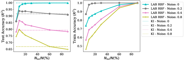
(a) Synthetic data $f_{1}$: 600 training data, 2 features

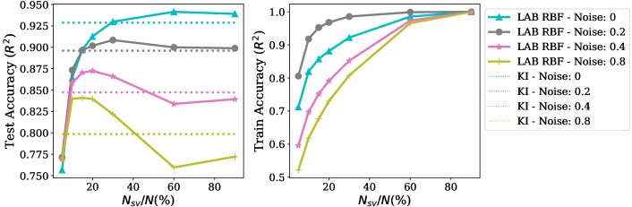
(b) Synthetic data $f_{2}$: 600 training data, 6 features

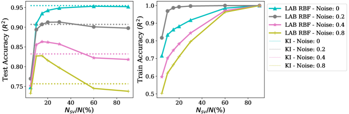
(c) Synthetic data $f_{3}$: 600 training data, 4 features

Figure 5: Effect of the number of support data on the performance of Algorithm 1. Three synthetic are used. Results of Algorithm 1 is presented in solid lines, and results of traditional kernel interpolation models are shown in dash lines. Various levels of noise are introduced into the training data.

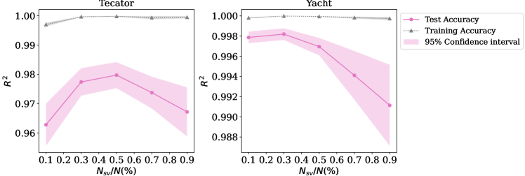
Figure 6: Effect of the number of support data on the performance of Algorithm 1. Two real datasets are used. Test accuracy is presented in solid lines, and training accuracy is shown in dash lines.

The impact of support data number. Figures 5 provide a detailed illustration of the impact of the support data number, displaying training and test accuracy curves in relation to the ratio of support data. To thoroughly evaluate the effect of noise, synthetic data with varying noise levels are considered in Figure 5, measured by the ratio of noise variance to the label variance. The results of the standard RBF kernel interpolation model (denoted as KI) are marked by the dashed lines. It is observed that KI is not robust to noise, as the accuracy sharply decreases with higher noise levels. In contrast, the proposed LAB RBF kernel-based ridgeless regression exhibits good robustness when an appropriate number of support data is selected. This validates our previous analysis, indicating that controlling support data number can enhance the model’s generalization ability.

Then, we utilize two small real datasets to closely examine the impact of the number of support data points. Figure 6 shows that having too few support data limits the capacity of the hypothesis space to fit the data, resulting in underfitting. Conversely, if the number of support data is excessively large, the remaining training data becomes insufficient to provide necessary information for learning bandwidths. This can cause the model to behave more like a simple kernel-based interpolation, making it less robust to noise and prone to overfitting, as evident from Figure 6. Therefore, selecting an appropriate number of support data is crucial to strike a balance between model complexity and overfitting.

Representational ability of the estimator. Four more real datasets with varying feature dimensions are studies in Figure 7, which illustrates the accuracy curve of kernel ridgeless regression with LAB RBF kernels in relation to the number of training data. As the number of training data increases, approximating all training data becomes more challenging, evident in the decline of the training accuracy curve. Conversely, the test accuracy improves with more information, indicating that the proposed algorithm gradually captures the underlying function. It is important to note that with only hundreds of support data, our approach effectively learns from tens of thousands of training data. For instance, with just 500 support data points, our method achieves over 99.5% training accuracy and 97.5% testing accuracy on the MNIST dataset, demonstrating the strong representational ability of the estimator.

In Figure7, results for different numbers of support data are also presented. It is observed that using more support data leads to better accuracy on the training dataset, which again aligns with our theoretical analysis. As the support data number increases, the capacity of the hypothesis space increases, allowing it to capture more complex underlying patterns in the data and resulting in higher training accuracy. However, its effect on generalization ability is not always positive. For instance, the function with 400 support data performs worse than that with only 200 support data in Figure 7 (b). As analyzed previously, a large number of support data implies a complex hypothesis space, which might bring larger sample error.

Comparison with other regression methods on more real datasets. The regression results of 10 methods on small-scale datasets are presented in Table 2. It is evident that greater model flexibility leads to improved regression accuracy, thus highlighting the benefits of flexible models. Notably, TL1 KRR outperforms RBF KRR in most datasets due to its indefinite nature. R-SVR-MKL, which considers a larger number of RBF kernels, exhibits much better performance than RBF KRR. While SVR-MKL, which considers a wider range of kernel types, achieves even higher accuracy compared to R-SVR-MKL. Among the neural network models, both ResNet and WNN demonstrate superior performance to the aforementioned methods. Advanced kernel methods, including Falkon, EigenPro3.0, and RFMs, also present significant improvement over traditionay kernel methods. Overall, LAB RBF achieves the highest regression accuracy, significantly increasing the $R^{2}$ compared to the baseline. Notably, LAB RBF performs better than ResNet in certain datasets, indicating that LAB RBF kernels offer sufficient flexibility and training bandwidths on the training dataset is indeed effective to enhance the model generalization ability.

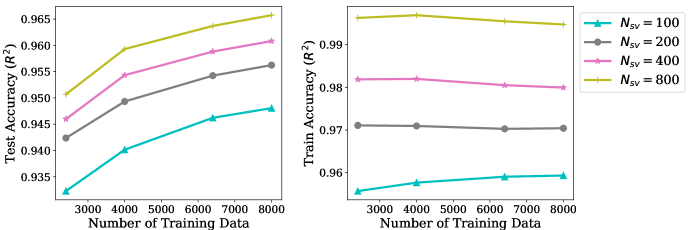
(a) Electricity: 10000 training data, 11 features

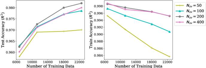
(b) Tomshardware: 28179 training data, 96 features

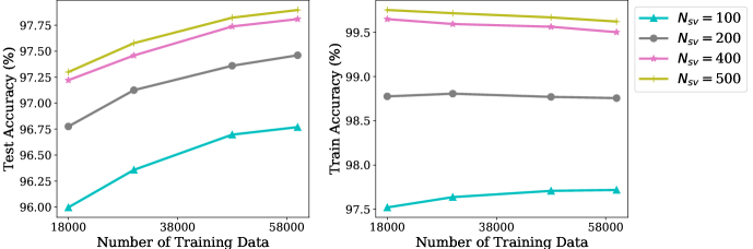
(c) MNIST: 60000 training data, 784 features

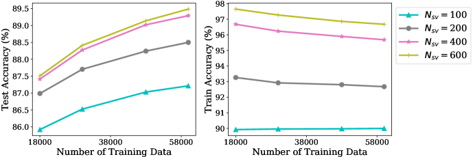
(d) FashionMNIST: 60000 training data, 784 features

Figure 7: Effect of the number of training data on the performance of Algorithm 1. Two regression and two classification real datasets are used. Results of models with different support data number is shown in different color.

Table 2 additionally reports the number of support vectors of kernel methods, which enables a more intuitive understanding of the sizes of decision models. Specifically, it provides the maximal support data number in Algorithm 1 for LAB RBF, and the predefined number of centers for Falkon, and the average number of support vectors for SVR methods. It should be noted that KRR uses all training data as support data, which results in a much larger complexity of the decision model compared to other kernel methods. This observation further underscores the advantage of enhancing kernel flexibility and learning kernels, as demonstrated by the compact size of the decision model achieved with our proposed LAB RBF kernel.

Traditional kernel-based algorithms are inefficient on large-scale datasets due to the matrix inverse operation on the large kernel matrix. Consequently, we compare our algorithm with three advanced kernel methods and two neural-network-based methods. The results are presented in Table 2, which more prominently underscores the capability of LAB RBF kernels in effectively reducing the required number of support data. Furthermore, it achieves a comparable level of regression accuracy to other advanced choices designed for such datasets. Notably, these advanced methods exhibit substantial model sizes. For instance, ResNet has a substantial number of parameters, and RFMs utilize all of the training data as support data. Although Falkon and EigenPro3.0 are based on the Nyström method, their reliance on symmetric kernel functions forces them to use a large amount of training data as support data to achieve high accuracy. In contrast, LAB RBF kernels maintain a comparatively low number of support data, attributed to the high flexibility provided by locally adaptive bandwidths and the kernel learning algorithm.

6 Related Works

Kernel ridgeless regression. The focus of this paper is on kernel ridgeless regression (Liang and Rakhlin, 2020), a kernel-based interpolation model that helps the understanding of benign overfitting phenomenon and over-parameterized models. Due to its solid theoretical foundation and straightforward algorithm, kernel ridgeless regression has continued to be widely studied in the machine learning community. Recent advancements have confirmed the phenomenon of benign overfitting, particularly in high-dimensional regimes (Hastie et al., 2022; Mei and Montanari, 2022). However, it is worth noting that such results often rely on the assumption of input dimensions tending towards infinity, a condition not always reflective of real-world datasets and target functions. Contrarily, in scenarios with lower dimensions (Buchholz, 2022) or fixed-dimensional setups (Beaglehole et al., 2023), interpolating kernel machines do not exhibit the benign overfitting phenomenon for commonly used kernels like Gaussian, Laplace, and Cauchy kernels.

RBF kernels with diverse bandwidths. RBF kernels that allow for different bandwidths in local regions have been investigated for a long time in the fields of kernel regression and kernel density estimation, e.g. Abramson (1982); Brockmann et al. (1993); Zheng et al. (2013). These pioneer works have focused on the selection of optimal bandwidths from data and have demonstrated that locally adaptive bandwidth estimators perform better than global bandwidth estimators in both theory and simulation studies. However, due to limited computing power and problem settings, these works have primarily analyzed one-dimensional algorithms and have not considered the generalization ability. In the field of machine learning, works like Steinwart et al. (2016); Hang and Steinwart (2021); Radhakrishnan et al. (2022) propose the use of feature-adaptive bandwidths and theoretically validate the improvement of flexible bandwidths. Successful experimental attempts have been achieved by directly applying asymmetric kernel functions (Moreno et al., 2003; Koide and Yamashita, 2006) or by incorporating them into existing kernel-based learning models along with asymmetric metric learning (Wu et al., 2010; Pintea et al., 2018). However, many of these studies lack a robust theoretical explanation, leaving the meaning of corresponding models and hypothesis space (no longer RKHS) still unknown. In this paper, for the first time, we demonstrate that LAB RBF kernels are actually involved with the integral space of RKHSs.

Table 1: Mean and standard of $R^{2}\;(\uparrow)$ of different regression methods on real datasets. The number of support vectors of different kernel-based methods are presented in blanket. The best and second-best results are indicated in bold and italic, respectively.

[b] Dataset Tecator Yacht Airfoil SML Parkinson Comp-active^a N=240,M=122 N=308,M=6 N=1503,M=5 N=4137,M=22 N=5875,M=20 N=8192,M=21 RBF KRR 0.9586$\pm$0.0071 (192) 0.9889$\pm$0.0025 (247) 0.8634$\pm$0.0248 (1203) 0.9779$\pm$0.0013 (3310) 0.8919$\pm$0.0091 (4700) 0.9822 (6554) TL1 KRR 0.9670$\pm$0.0113 (192) 0.9705$\pm$0.0033 (247) 0.9464$\pm$0.0065 (1203) 0.9947$\pm$0.0005 (3310) 0.9475$\pm$0.0034 (4700) 0.9801 (6554) R-SVR-MKL 0.9711$\pm$0.0212 (174.2) 0.9945$\pm$0.0008 (224.7) 0.9201$\pm$0.01099 (953.1) 0.9959$\pm$0.0006 (2844) 0.9032$\pm$0.0122 (4047) 0.9834 (1397) SVR-MKL 0.9698$\pm$0.0157 (160.7) 0.9957$\pm$0.0022 (144.5) 0.9535$\pm$0.0042 (1035) 0.9970$\pm$ 0.0006 (1424) 0.9011$\pm$0.0110 (3759) 0.9829 (1423) EigenPro3.0 0.9758$\pm$0.0029 (192) 0.9944$\pm$0.0036 (247) 0.9262$\pm$0.0166 (1203) 0.9934$\pm$0.0009 (3310) 0.9260$\pm$0.0079 (4700) 0.9830 (6554) RFMs 0.9811$\pm$0.0078 (192) 0.9947$\pm$0.0018 (247) 0.9394 $\pm$0.0079 (1203) 0.9960$\pm$0.0007 (3310) 0.9988$\pm$0.0004 (4700) 0.9852 (6554) Falkon 0.9769$\pm$0.0086 (100) 0.9982$\pm$0.0024 (200) 0.9377 $\pm$0.0067 (900) 0.9960$\pm$0.0007 (2000) 0.9492$\pm$0.0063 (4000) 0.9808 (1500) ResNet 0.9841$\pm$0.0067 0.9940$\pm$0.0003 0.9538$\pm$0.0066 0.9976$\pm$0.0004 0.9906$\pm$0.0048 0.9836 WNN 0.9875$\pm$0.0044 0.9924$\pm$0.0025 0.9128$\pm$0.0089 0.9926$\pm$0.0008 0.9139$\pm$0.0055 0.9817 LAB RBF 0.9782$\pm$0.0151 (76) 0.9980$\pm$0.0009 (73) 0.9649$\pm$0.0091 (800) 0.9985$\pm$0.00007 (400) 0.9990$\pm$0.0005 (400) 0.9835 (70)

• The test set of Comp-activ is pre-given.

• Notations N, M denote the data number and the feature dimension, respectively.

Table 2: Mean and standard of $R^{2}(\uparrow)$ of different algorithms in large-scale datasets. The number of support vectors of different kernel-based methods are presented in blanket. The best and second-best results are indicated in bold and italic, respectively.

Dataset	Electrical	KC House	TomsHardware
	N=10000,M= 11	N=21623,M=14	N=28179,M=96
WNN	0.9617$\pm$0.0027	0.8501$\pm$0.0194	0.9248$\pm$0.0303
ResNet	0.9705$\pm$0.0025	0.8823$\pm$0.0117	0.9697$\pm$0.0021
EigenPro3.0	0.9513$\pm$0.0024 (8000)	0.8636$\pm$0.0119 (17291)	0.9436$\pm$0.0282 (20000)
RFMs	0.9582$\pm$0.0028 (8000)	0.9008$\pm$0.0072 (17291)	0.9115$\pm$0.0031 (22544)
Falkon	0.9532$\pm$0.0025 (3000)	0.8640$\pm$0.0145 (5000)	0.9001$\pm$0.0143 (5000)
LAB RBF	0.9654$\pm$0.0034 (300)	0.9103$\pm$0.0061(550)	0.9809$\pm$0.0028 (500)

Asymmetric kernel-based learning. Existing research in asymmetric kernel learning has primarily proposed frameworks based on SVD (Suykens, 2016) and least square SVM (He et al., 2023). However, for regression tasks, current works Mackenzie and Tieu (2004); Pintea et al. (2018) directly incorporate asymmetric kernels into symmetric-kernel-based learning models, lacking interpretability. Additionally, other works primarily focus on interpreting associated optimization models (Wu et al., 2010; Lin et al., 2022), where the corresponding functional space is regarded as a Reproducible Kernel Banach Space. This, however, is not currently applicable to LAB RBF kernels, as their reproducible property remains undetermined. Despite notable progress in theory, current applications of asymmetric kernel matrices often rely on datasets (e.g. the directed graph in He et al. (2023)) or recognized asymmetric similarity measures (e.g. the Kullback-Leibler kernels in Moreno et al. (2003)) This yields improved performance in specific scenarios but leaving a significant gap in addressing diverse datasets. With the help of trainable LAB RBF kernels, this paper proposes a robust groundwork for utilizing asymmetric kernels in tackling general regression tasks.

7 Conclusion

In this paper, we enhance the kernel ridgeless regression with trainable LAB RBF kernels and investigated it from the approximation theory viewpoint. The LAB RBF kernel is highly flexible due to its over-parameterized form, where the bandwidths are data-adaptive and can vary depending on the size of the training data. While the 1-dimensional case of the LAB RBF kernel has been previously studied in statistics, its high-dimensional case and application in machine learning had not been explored. We presented an iterative learning algorithm based on a ridgeless model to determine the bandwidths of the LAB RBF kernel, with controllable support vectors and applicable gradient methods for training the bandwidths. Experimental results on real regression datasets show that our algorithm achieves state-of-the-art accuracy. This demonstrates the benefits of increasing kernel flexibility, and verifies the effectiveness of our proposing learning algorithm.

To investigate the source of the generalization ability in the proposed model without explicit regularization, we introduced the $\ell_{0}$-regularized model in the integral space of RKHSs. The optimal function of this model is equivalent to the interpolation function derived by a well-learned LAB RBF kernel. Through the analysis of this model, we gained insights into the advantages of kernel ridgeless regression with LAB RBF kernels. Our theoretical analysis was based on the standard error decomposition technique, where we utilized the latest results on $\ell_{q}$-regularization models, conclusions on Rademacher chaos complexity of Gaussian kernels, and a refined iteration technique for $\ell_{0}$-regularization. We demonstrated that at the optimal point of our proposed $\ell_{0}$-regularized model, the integral space of RKHSs reduces to a sum space of RKHSs, enabling us to bound the sample error in a complex space.

Our analysis revealed that the excellent representation ability of the proposed model is due to the large hypothesis spaces introduced by LAB RBF kernels, i.e., the integral space of RKHSs, which enables our algorithm to interpolate the training dataset with only a few support vectors. Meanwhile, the natural sparsity of LAB RBF kernels, controlled by the number of support vectors, guarantees their good generalization ability, as seen from the analysis of the sample error. The number of support vectors plays a crucial role in the trade-off between the approximation ability in the training data and the generalization ability in the test data, which is also validated by our experimental results.

Considering the fundamental role of non-Mercer and asymmetric kernels in modern deep learning architectures like transformers (Wright and Gonzalez, 2021; Chen et al., 2024), we hope our analysis of kernel ridgeless regression and LAB RBF kernels will inspire further research on asymmetric kernel learning and the integral space of RKHSs in machine learning.

Acknowledgments and Disclosure of Funding

The author would like to thank Mingzhen He for his insightful suggestions on this work. The research leading to these results received funding from the European Research Council under the European Union’s Horizon 2020 research and innovation program / ERC Advanced Grant E-DUALITY (787960). This paper reflects only the authors’ views and the Union is not liable for any use that may be made of the contained information. This work was also supported in part by Research Council KU Leuven: iBOF/23/064; Flemish Government (AI Research Program). Johan Suykens is also affiliated with the KU Leuven Leuven.AI institute. Additionally, this work received partial support from the National Natural Science Foundation of China under Grants 62376155 and 12171093, as well as from the Shanghai Science and Technology Program under Grants 22511105600, 20JC1412700, and 21JC1400600. Further support was obtained from the Shanghai Municipal Science and Technology Major Project under Grant 2021SHZDZX0102. Xiaolin Huang and Lei Shi are the corresponding authors.

Appendix A Proof of Theorem 1

Here we present the proof of Theorem 1.

Proof  Based on Equation (6), we can express ${\bf w}^{*}$ as:

$${\bf w}^{*} =\psi({\bf X})(\phi^{\top}({\bf X})\psi({\bf X})+\lambda{\bf I}_{N})^{-1}{\bf Y} \overset{(a)}{=}(\lambda{\bf I}_{F}+\psi({\bf X})\phi^{\top}({\bf X}))^{-1}\psi({\bf X}){\bf Y}$$ (38)

where equation (a) is derived from (6) with ${\bf A}={\bf I}_{F},\;{\bf B}=\psi({\bf X}),\;{\bf C}=\phi^{\top}({\bf X}),\;{\bf D}={\bf I}_{N}$. Similarly, for ${\bf v}^{*}$, we have

$${\bf v}^{*} =\phi({\bf X})(\psi^{\top}({\bf X})\phi({\bf X})+\lambda{\bf I}_{N})^{-1}{\bf Y} \overset{(b)}{=}(\lambda{\bf I}_{F}+\phi({\bf X})\psi^{\top}({\bf X}))^{-1}\phi({\bf X}){\bf Y},$$ (39)

where equation (b) again applies (6) with ${\bf A}={\bf I}_{F},\;{\bf B}=\phi({\bf X}),\;{\bf C}=\psi^{\top}({\bf X}),\;{\bf D}={\bf I}_{N}$. Take the derivation of the objective function with respect to ${\bf w}$ and ${\bf v}$ at point $({\bf w}^{*},{\bf v}^{*})$, we observe:

$$\frac{\partial L}{\partial{\bf w}}|_{{\bf w}={\bf w}^{*}\atop{\bf v}={\bf v}^{*}} =(\lambda{\bf I}_{F}+\phi({\bf X})\psi^{\top}({\bf X}))(\lambda{\bf I}_{F}+\phi({\bf X})\psi^{\top}({\bf X}))^{-1}\phi({\bf X}){\bf Y}-\phi({\bf X}){\bf Y}=0,$$

$$\frac{\partial L}{\partial{\bf v}}|_{{\bf w}={\bf w}^{*}\atop{\bf v}={\bf v}^{*}} =(\lambda{\bf I}_{F}+\psi({\bf X})\phi^{\top}({\bf X}))(\lambda{\bf I}_{F}+\psi({\bf X})\phi^{\top}({\bf X}))^{-1}\psi({\bf X}){\bf Y}-\psi({\bf X}){\bf Y}=0.$$

This verifies that the point $({\bf w}^{*},{\bf v}^{*})$ satisfies the stationarity condition.  

Appendix B Alternative derivation of Asymmetric KRR and Function Explanation

We can also derive a similar result in Theorem 1 in a LS-SVM-like approach (Suykens and Vandewalle, 1999), from which we can better understand the relationship between the two regression functions. By introducing error variables $e_{i}=y_{i}-\phi({\bf x}_{i})^{\top}{\bf w}$ and $r_{i}=y_{i}-\psi({\bf x}_{i})^{\top}{\bf v}$, the last term in (7) equals to $\sum_{i}e_{i}r_{i}$. According to this result, we have the following optimization:

$$\min_{{\bf w},{\bf v},{\bf e},{\bf r}} \lambda{\bf w}^{\top}{\bf v}+\sum_{i=1}^{N}e_{i}r_{i}$$ (40)

$$\mathrm{s.t.} r_{i}=y_{i}-\psi({\bf x}_{i})^{\top}{\bf v},\quad\forall i=1,2,\cdots,N,$$

$$e_{i}=y_{i}-\phi({\bf x}_{i})^{\top}{\bf w},\quad\forall i=1,2,\cdots,N.$$

From the Karush-Kuhn-Tucker (KKT) conditions (Boyd and Vandenberghe, 2004), we can obtain the following result on the KKT points.

Theorem 16

Let ${\bm{\alpha}}=[\alpha_{1},\cdots,\alpha_{N}]^{\top}\in\mathbb{R}^{N}$ and ${\bm{\beta}}=[\beta_{1},\cdots,\beta_{N}]^{\top}\in\mathbb{R}^{N}$ be Lagrange multipliers of constraints $r_{i}=y_{i}-\psi({\bf x}_{i})^{\top}{\bf v}$ and $e_{i}=y_{i}-\phi({\bf x}_{i})^{\top}{\bf w},\forall i=1,\cdots,N$, respectively. Then one of the KKT points of (40) is

$${\bf w}^{*}=\frac{1}{\lambda}\psi({\bf X}){\bm{\alpha}}^{*},\quad\quad{\bf v}^{*}=\frac{1}{\lambda}\phi({\bf X}){\bm{\beta}}^{*},$$

$${\bf e}^{*}={\bm{\alpha}}^{*}=\lambda(\phi^{\top}({\bf X})\psi({\bf X})+\lambda{\bf I}_{N})^{-1}{\bf Y},$$

$${\bf r}^{*}={\bm{\beta}}^{*}=\lambda(\psi^{\top}({\bf X})\phi({\bf X})+\lambda{\bf I}_{N})^{-1}{\bf Y}.$$

The proof is presented in Appendix C. This model shares a close relationship with existing models. For instance, by modifying the regularization term from ${\bf w}^{\top}{\bf v}$ to ${\bf w}^{\top}{\bf w}+{\bf v}^{\top}{\bf v}$ and flipping the sign of $\sum_{i=1}^{N}e_{i}r_{i}$, we arrive at the kernel partial least squares model as outlined in Hoegaerts et al. (2004). In the specific case where $\psi=\phi$, its KKT conditions align with those of the LS-SVM setting for ridge regression (Saunders et al., 1998; Suykens et al., 2002). Furthermore, under the same condition of $\psi=\phi$ and when the regularization parameter is set to zero, it reduces to ordinary least squares regression (Hoegaerts et al., 2005).

With the aid of error variables ${\bf e}$ and ${\bf r}$, a clearer perspective on the relationship between $f_{1}$ and $f_{2}$ emerges. As clarified in Theorem 16, the approximation error on training data is equal to the value of dual variables, a computation facilitated through the kernel trick. Consequently, this reveals that $f_{1}$ and $f_{2}$ typically diverge when $\phi$ and $\psi$ are not equal, as they exhibit distinct approximation errors. A complementary geometric insight arises from the term $\sum_{i=1}^{N}e_{i}r_{i}$ within the objective function. This signifies that, in practice, $f_{1}$ and $f_{2}$ tend to approach the target $y$ from opposite directions because the signs in their approximation errors tend to be dissimilar. For practical applications, one may opt for the regression function with the smaller approximation error.

Appendix C Proof of Theorem 16

Here we present the proof of Theorem 16.

Proof 

The Lagrangian of (40) is

$$\mathcal{L}=\lambda{\bf w}^{\top}{\bf v}+\sum_{i=1}^{N}e_{i}r_{i}+\sum_{i}\beta_{i}(y_{i}-e_{i}-\phi({\bf x}_{i})^{\top}{\bf w})+\sum_{i}\alpha_{i}(y_{i}-r_{i}-\psi({\bf x}_{i})^{\top}{\bf v}),$$ (41)

where ${\bm{\alpha}}\in\mathbb{R}^{N}$ and ${\bm{\beta}}\in\mathbb{R}^{N}$ are Lagrange multipliers. The KKT conditions lead to

$$\frac{\partial\mathcal{L}}{\partial{\bf v}}=\lambda{\bf w}-\psi({\bf X}){\bm{\alpha}}=0 \Longrightarrow{\bf w}=\frac{1}{\lambda}\psi({\bf X}){\bm{\alpha}},$$

$$\frac{\partial\mathcal{L}}{\partial{\bf w}}=\lambda{\bf v}-\phi({\bf X}){\bm{\beta}}=0 \Longrightarrow{\bf v}=\frac{1}{\lambda}\phi({\bf X}){\bm{\beta}},$$

$$\frac{\partial\mathcal{L}}{\partial r_{i}}=e_{i}-\alpha_{i}=0 \Longrightarrow e_{i}=\alpha_{i},$$

$$\frac{\partial\mathcal{L}}{\partial e_{i}}=r_{i}-\beta_{i}=0 \Longrightarrow r_{i}=\beta_{i},$$

$$\frac{\partial\mathcal{L}}{\partial\beta_{i}}=y_{i}-e_{i}-\phi({\bf x}_{i})^{\top}{\bf w}=0 \Longrightarrow e_{i}=y_{i}-\phi({\bf x}_{i})^{\top}{\bf w},$$

$$\frac{\partial\mathcal{L}}{\partial\alpha_{i}}=y_{i}-r_{i}-\psi({\bf x}_{i})^{\top}{\bf v}=0 \Longrightarrow r_{i}=y_{i}-\psi({\bf x}_{i})^{\top}{\bf v}.$$

Substitute the first four lines into the last two lines, we can eliminate primal variables ${\bf w},{\bf v},{\bf e},{\bf r}$:

$${\bm{\alpha}}^{*}={\bf Y}-\frac{1}{\lambda}\phi({\bf X})^{\top}\psi({\bf X}){\bm{\alpha}}^{*} \Longrightarrow{\bm{\alpha}}^{*}=\lambda(\lambda{\bf I}_{N}+\phi({\bf X})^{\top}\psi({\bf X}))^{-1}{\bf Y},$$

$${\bm{\beta}}^{*}={\bf Y}-\frac{1}{\lambda}\psi({\bf X})^{\top}\phi({\bf X}){\bm{\beta}}^{*} \Longrightarrow{\bm{\beta}}^{*}=\lambda(\lambda{\bf I}_{N}+\psi({\bf X})^{\top}\phi({\bf X}))^{-1}{\bf Y}.$$

Thus, we get the result in Theorem 16 and the proof is completed.  

Appendix D Proof of Proposition 3

Here we present the proof of Proposition 3.

Proof  The proof is achieved by constructing a equivalent constrained version of optimization (16).

$$f_{\bf z}=\arg\min_{\begin{subarray}{c}f\in\mathcal{H}_{\Omega}\\ \{{\bm{\theta}}_{i}\}\subset\Omega\end{subarray}}\mathcal{E}_{\bf z}({f})\quad\;\mathrm{s.t.}\;\;\mathcal{R}_{0}(f)=N_{sv},\;\;{\mu}({\bm{\sigma}})=\sum_{i=1}^{N_{sv}}\delta({\bm{\sigma}}-\theta_{i}).$$ (42)

We firstly show that $f_{\mathcal{Z}_{sv},{\bm{\Theta}}}$ belongs to this integral space. Recall that $f_{\mathcal{Z}_{sv},{\bm{\Theta}}}$ has an analytical formulation as presented in (43). Let ${\bm{\Theta}}=\{{\bm{\theta}}_{i}\}_{i=1}^{N_{sv}}$ denotes the bandwidth set of these support data. Then there exists a interval $\Omega\subset\mathbb{R}^{M}_{+}$ satisfying that $\theta_{i}\in\Omega,\forall i$ as ${\bm{\Theta}}$ is a discrete set. Without loss of generality, we assume that $\|{\bm{\alpha}}\|_{2}<\infty$. Then define

$$\tilde{f}_{\theta_{i}}({\bf t})\triangleq\alpha_{i}\exp\{-\|\theta_{i}\odot({\bf t}-{\bf x}_{i})\|_{2}^{2}\}=\alpha_{i}\mathcal{K}_{{\bm{\theta}}_{i}}({\bf t},{\bf x}_{i})$$ (43)

and $\tilde{\mu}({\bm{\sigma}})=\sum_{i=1}^{N_{sv}}\delta({\bm{\sigma}}-\theta_{i})$, where $\delta(\cdot)$ denotes the Dirac delta function. Under this definition we have $f_{\mathcal{Z}_{sv},{\bm{\Theta}}}({\bf x})=\int_{\bm{\sigma}}\tilde{f}_{\bm{\sigma}}({\bf x})d\tilde{\mu}({\bm{\sigma}})$ and

$$\int_{{\bm{\sigma}}\in\Omega}\|\tilde{f}_{\bm{\sigma}}\|_{\mathcal{H}_{\bm{\sigma}}}d\tilde{\mu}({\bm{\sigma}})=\sum_{i=1}^{N_{sv}}\|\tilde{f}_{\theta_{i}}\|_{\mathcal{H}_{\theta_{i}}}\leq\|{{\bm{\alpha}}}\|_{2}<\infty,$$

which indicates that $f_{\mathcal{Z}_{sv},{\bm{\Theta}}}\in\mathcal{H}_{\Omega}.$

The formulation in (43) means that for every kernel $\mathcal{K}_{{\bm{\theta}}_{i}}$, only one coefficient are non-zero. Then recall the definition in (15), we have $\mathcal{R}_{0}(f_{\mathcal{Z}_{sv},{\bm{\Theta}}})=N_{sv}$, indicating that $f_{\mathcal{Z}_{sv},{\bm{\Theta}}}$ is a feasible solution of problem (42). recall the stopping condition in the dynamic strategy (14), we have $0<\mathcal{E}_{\bf z}(f_{\mathcal{Z}_{sv},{\bm{\Theta}}})-\mathcal{E}_{\bf z}({f}_{{\bf z}})\leq B.$ Finally, as all constrain in (42) are equalities, we can always find a suitable $\lambda>0$ such that optimization (16) shares the same optimizer as that of (42). That is, $f_{{\bf z}}=f_{{\bf z},\lambda}$. Then, we obtain the desired conclusion and complete the proof.

 

Appendix E Experiment Details

The used datasets can be download from:

• Tecator: http://lib.stat.cmu.edu/datasets/tecator.

• Yacht: https://archive.ics.uci.edu/dataset/243/yacht+hydrodynamics.

• Airfoil: https://archive.ics.uci.edu/dataset/291/airfoil+self+noise.

• SML: https://archive.ics.uci.edu/dataset/274/sml2010.

• Parkinson: https://archive.ics.uci.edu/dataset/189/parkinsons+telemonitoring.

• Comp-activ: https://www.cs.toronto.edu/~delve/data/comp-activ/desc.html.

• TomsHardware: https://archive.ics.uci.edu/dataset/248/buzz+in+social+media.

• KC House: https://www.kaggle.com/datasets/shivachandel/kc-house-data.

• Electrical: https://archive.ics.uci.edu/dataset/471/electrical+grid+stability+simulated+data.

• MNIST:http://yann.lecun.com/exdb/mnist/

• Fashion-MNIST: https://github.com/zalandoresearch/fashion-mnist

Appendix F Details of Compared methods and hyper-parameter setting.

Compared methods: nine regression methods are compared in this experiment, including:

• RBF KRR (Vovk, 2013): classical kernel ridge regression with conventional RBF kernels, served as the baseline.

• TL1 KRR: classical kernel ridge regression employing an indefinite kernel named Truncated $\ell_{1}$ kernel (Huang et al., 2018). The expression of TL1 kernel is $\mathcal{K}({\bf x},{\bf x}^{\prime})=\max\{\rho-\|{\bf x}-{\bf x}^{\prime}\|_{1},0\},$ where $\rho>0$ is a pre-given hyper-parameter. The TL1 kernel is a piecewise linear indefinite kernel and is expected to be more flexible and have better performance than the conventional RBF kernel.

• SVR-MKL: Multiple kernel learning applied on support vector regression. The kernel dictionary includes RBF kernels, Laplace kernels, and polynomial kernels. Results for R-SVR-MKL with only RBF kernels are also provided. The implementation of MKL is available in the Python package MKLpy (Aiolli and Donini, 2015; Lauriola and Aiolli, 2020).

• Falkon (Rudi et al., 2017; Meanti et al., 2022): An advanced and well-developed algorithm for KRR that employs hyper-parameter tuning techniques to enhance accuracy and utilizes Nyström approximation to reduce the number of support data points, enabling it to handle large-scale datasets. We used the public code of Falkon, available at https://github.com/FalkonML/falkon.

• EigenPro3.0 (Abedsoltan et al., 2023): An advanced general kernel machine for large datasets, utilizing Nystöm methods and projected dual preconditioned SGD. We used the public code of EigenPro3.0, available at https://github.com/EigenPro/EigenPro3.

• RFMs (Radhakrishnan et al., 2022): Recursive feature machines is advanced kernel methods which utilizes the mechanism of deep feature learning, resulting high efficient algorithms and ability to handle large datasets. We used the public code of RFMs, available at https://github.com/aradha/recursive_feature_machines.

• ResNet: The regression version of ResNet follows the structure in Chen et al. (2020), and the code is available in https://github.com/DowellChan/ResNetRegression.

• WNN: The regression version of a wide neural network, which is fully-connected and has only one hidden layer.

Implementation details. Among the compared methods, Kernel Ridge Regression (KRR) stands as the fundamental technique that combines the Tikhonov regularized model with the kernel trick. The coefficients of kernels for both SVR-MKL and R-SVR-MKL are calculated following the approach in EasyMKL (Aiolli and Donini, 2015). For Falkon, the code is available at https://github.com/FalkonML/falkon. LAB RBF, ResNet, and WNN are optimized using gradient methods with varying hyper-parameters such as initial points, learning rate, and batch size. The initial weights of both ResNet and WNN are set according to the Kaiming initialization introduced in He et al. (2015). In the subsequent experiments, the Adam optimizer is initially used, and upon stopping, the SGD optimizer is applied. Early stopping is implemented for the training of ResNet and WNN, where $10\%$ of the training data is sampled to form a validation set, and validation loss is assessed every epoch. The epoch with the best validation loss is selected for testing. Detailed hyper-parameters of all compared methods are provided in Table 3 (for small-scale datasets) and Table 4 (for large-scale datasets).

The regression version of ResNet follows the structure in Chen et al. (2020), which has available code in https://github.com/DowellChan/ResNetRegression. Following the structures in Chen et al. (2020), the ResNet block has two types: Identity Block (where the dimension of input and output are the same) and Dense Block (where the dimension of input and output are different). The details of these two block are presented in Figure 8. Considering the different dataset sizes, we use two structures of ResNet in our experiments, denoted by ResNet and ResNetSmall. For the ResNet, we use two Dense Blocks (M-W-100) and two Identity Block (100-100-100) and a linear predict layer (100-1). For the ResNetSmall, we use two Dense Blocks (M-W-50) and a linear predict layer (50-1). Here W is a pre-given width for the network.

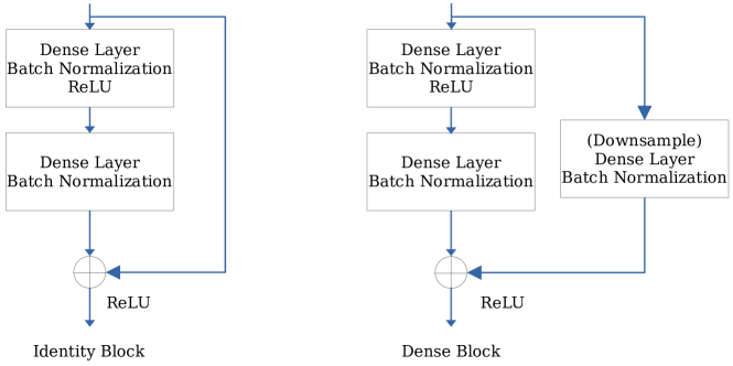
Figure 8: The structures of Identity block and Dense block.

Table 3: Hyper-parameters of eight regression methods for real datasets.

[b] Hyper-parameters Tecator Yacht Airfoil SML Parkinson Comp_activ LAB RBF lr 0.001 0.01 0.01 0.05 0.001 0.001 Batch size 16 128 128 128 128 128 $\sigma_{0}$ 0.5 3 10 50 30 0.1 R-SVR-MKL C 1000 1000 1 1000 10 1 $\epsilon$ 0.001 0.001 0.01 0.001 0.01 0.01 Dictionary RBF kernels: $[100,50,10,1,0.1,0.01,0.001]$ SVR-MKL C 1000 1000 100 1000 1000 1000 $\epsilon$ 0.01 0.01 0.01 0.01 0.01 0.01 Dictionary RBF kernels: $[100,1,0.1,0.001]$ Laplace kernels: $[100,1,0.1,0.001]$ Polynomial kernels: $[1,2,4,10]$ RBF KRR $\sigma$ 1 5 80 5 20 10 $\lambda$ 0.01 0.001 0.001 0.01 0.001 0.001 TL1 KRR $\rho$ 98 6 2.5 22 14 15 $\lambda$ 0.001 0.001 0.001 0.1 0.01 0.001 Falkon $\lambda$ 1e-6 1e-7 1e-6 1e-5 1e-7 1e-6 Center^a 100 200 900 2000 4000 1500 $\sigma$ 10 1 2 1 0.7 2.5 EigenPro3.0 $\sigma$ 3 1 0.5 1 0.5 10 Center^a 197 247 1203 3310 4700 6554 ResNet lr 0.001 0.001 0.001 0.001 0.001 0.001 Batch size 32 32 128 128 128 128 Structure (Width)^b 2(500) 2(500) 1(1000) 1(1000) 1(500) 1(2000) WNN lr 0.001 0.001 0.001 0.001 0.001 0.001 Batch size 32 32 128 128 128 128 Width 800 500 6000 1500 3000 9000

• The center number of Nyström approximation.

• Structure 1:$M-W-100-100-100-1$, Structure 2: $M-W-50-1$.

Table 4: Hyper-parameters of four regression methods for real datasets.

	Hyper-parameters	TomsHardware	Electrical	KC House
LAB RBF	lr	0.001	0.001	0.001
	Batch size	256	256	256
	$\sigma_{0}$	0.1	0.1	1
Falkon	$\lambda$	1e-6	1e-6	1e-6
	Center	3000	3000	5000
	$\sigma$	2	10	5
EigenPro3.0	$\sigma$	7	1	5
	Center	20000	8000	17291
ResNet	lr	0.001	0.001	0.001
	Batch size	128	256	256
	Structure (Width)a	1(3000)	1(2000)	1(2000)
WNN	lr	0.01	0.01	0.01
	Batch size	128	256	128
	Width	3000	3000	5000

• Structure 1:$M-W-100-100-100-1$.

Appendix G Study on different selection strategy of initial support data

The selection of support data has the significant influence on the performance of the proposed algorithm. In light of this, we have introduced a dynamic strategy aimed at mitigating the impact of initial support data selection in the manuscript.

In this section, we delve deeper into the effects of various methods for selecting initial support data and assess the efficacy of the introduced dynamic strategy. We will explore three different approaches to initial data selection: two rational methods (Y-based and X-based) and one irrational method (Extreme Y).

• Y-based (utilized in the manuscript): data is sorted based on their labels, and support data is uniformly selected.

• X-based: k-means is applied to the training data to identify cluster centers, followed by the selection of data points closest to these centers.

• Extreme Y: data is sorted based on their labels, and those with the largest Y values are selected.

Table 5 presents the performance of Algorithm 1 with these selection methods on Yacht and Parkinson datasets. The results indicate that the poor selection method does have a detrimental impact on our performance, particularly evident in the case of Yacht where we struggle to fit the data. In contrast, the other two sensible methods demonstrate good and comparable performance.

In order to further improve, we introduce a dynamic strategy at the end of Section 3. In this strategy, we dynamically incorporate hard samples into the support dataset. We then integrate these approaches with the proposed dynamic strategy to evaluate its effectiveness, of which the results are presented in Table 6. Based on these results, it is evident that the proposed dynamic strategy has a significantly positive impact on performance. It not only enhances accuracy but also reduces variance, resulting in more stable solutions. Even with the bad selection selection, the final performance is improved to a satisfactory level.

Table 5: Performance of Algorithm1 with different selection methods of initial support data.

Dataset	Yacht	Yacht	Yacht	Parkinson	Parkinson	Parkinson
Selection Approach	Extreme Y	Y-based	X-based	Extreme Y	Y-based	X-based
Mean of $R^{2}$	0.0012	0.9957	0.9953	0.8115	0.9921	0.9928
Std of $R^{2}$	0.4805	0.0025	0.0032	0.0126	0.0015	0.0016

Table 6: Performance of Algorithm1 with dynamic strategy and different selection methods of initial support data.

Dataset	Yacht	Yacht	Yacht	Parkinson	Parkinson	Parkinson
Selection Approach	Extreme Y	Y-based	X-based	Extreme Y	Y-based	X-based
Mean of R2	0.9961	0.9982	0.9981	0.9712	0.9972	0.9966
Std of R2	0.0126	0.0015	0.0016	0.0049	0.0007	0.0013

References

• Abedsoltan et al. (2023) A. Abedsoltan, M. Belkin, and P. Pandit. Toward large kernel models. In Proceedings of the 40th International Conference on Machine Learning, volume 202 of Proceedings of Machine Learning Research, pages 61–78. PMLR, 23–29 Jul 2023.
• Abramson (1982) I. Abramson. On bandwidth variation in kernel estimates-a square root law. Annals of Statistics, 10:1217–1223, 1982.
• Adlam and Pennington (2020) B. Adlam and J. Pennington. The neural tangent kernel in high dimensions: Triple descent and a multi-scale theory of generalization. In International Conference on Machine Learning, pages 74–84. PMLR, 2020.
• Aiolli and Donini (2015) F. Aiolli and M. Donini. Easymkl: a scalable multiple kernel learning algorithm. Neurocomputing, 169:215–224, 2015.
• Allen-Zhu et al. (2019a) Z. Allen-Zhu, Y. Li, and Y. Liang. Learning and generalization in overparameterized neural networks, going beyond two layers. Advances in neural information processing systems, 32, 2019a.
• Allen-Zhu et al. (2019b) Z. Allen-Zhu, Y. Li, and Z. Song. A convergence theory for deep learning via over-parameterization. In International conference on machine learning, pages 242–252. PMLR, 2019b.
• Aronszajn (1950) N. Aronszajn. Theory of reproducing kernels. Transactions of the American Mathematical Society, 68(3):337–404, 1950.
• Arzamasov (2018) V. Arzamasov. Electrical Grid Stability Simulated Data . UCI Machine Learning Repository, 2018. DOI: https://doi.org/10.24432/C5PG66.
• Asuncion and Newman (2007) A. Asuncion and D. Newman. UCI machine learning repository, 2007.
• Bach (2022) F. Bach. Information theory with kernel methods. IEEE Transactions on Information Theory, 69(2):752–775, 2022.
• Bartlett et al. (2020) P. L. Bartlett, P. M. Long, G. Lugosi, and A. Tsigler. Benign overfitting in linear regression. Proceedings of the National Academy of Sciences, 117(48):30063–30070, 2020.
• Beaglehole et al. (2023) D. Beaglehole, M. Belkin, and P. Pandit. On the inconsistency of kernel ridgeless regression in fixed dimensions. SIAM Journal on Mathematics of Data Science, 5(4):854–872, 2023.
• Belkin et al. (2018) M. Belkin, S. Ma, and S. Mandal. To understand deep learning we need to understand kernel learning. In International Conference on Machine Learning, pages 541–549. PMLR, 2018.
• Boyd and Vandenberghe (2004) S. P. Boyd and L. Vandenberghe. Convex optimization. Cambridge university press, 2004.
• Brockmann et al. (1993) M. Brockmann, T. Gasser, and E. Herrmann. Locally adaptive bandwidth choice for kernel regression estimators. Journal of the American Statistical Association, 88:1302–1309, 1993.
• Brooks et al. (2014) T. Brooks, D. Pope, and M. Michael. Airfoil Self-Noise. UCI Machine Learning Repository, 2014. DOI: https://doi.org/10.24432/C5VW2C.
• Buchholz (2022) S. Buchholz. Kernel interpolation in sobolev spaces is not consistent in low dimensions. In Conference on Learning Theory, pages 3410–3440. PMLR, 2022.
• Cao et al. (2022) Y. Cao, Z. Chen, M. Belkin, and Q. Gu. Benign overfitting in two-layer convolutional neural networks. Advances in neural information processing systems, 35:25237–25250, 2022.
• Chatterji and Long (2021) N. S. Chatterji and P. M. Long. Finite-sample analysis of interpolating linear classifiers in the overparameterized regime. The Journal of Machine Learning Research, 22(1):5721–5750, 2021.
• Chen et al. (2020) D. Chen, F. Hu, G. Nian, and T. Yang. Deep residual learning for nonlinear regression. Entropy, 22(2):193, 2020.
• Chen et al. (2004) D. R. Chen, Q. Wu, Y. Ying, and D. X. Zhou. Support vector machine soft margin classifiers: Error analysis. Journal of Machine Learning Research, 5(3):1143–1175, 2004.
• Chen et al. (2024) Y. Chen, Q. Tao, F. Tonin, and J. A. K. Suykens. Primal-attention: Self-attention through asymmetric kernel svd in primal representation. Advances in Neural Information Processing Systems, 36, 2024.
• Cherkassky et al. (1996) V. Cherkassky, D. Gehring, and F. Mulier. Comparison of adaptive methods for function estimation from samples. IEEE Transactions on Neural Networks, 7(4):969–984, 1996.
• Cucker and Zhou (2007) F. Cucker and D. X. Zhou. Learning Theory: An Approximation Theory Viewpoint. Cambridge University Press Cambridge, 2007.
• Deng (2012) L. Deng. The mnist database of handwritten digit images for machine learning research [best of the web]. IEEE Signal Processing Magazine, 29(6):141–142, 2012.
• Eberts and Steinwart (2011) M. Eberts and I. Steinwart. Optimal learning rates for least squares svms using gaussian kernels. Advances in neural information processing systems, 24, 2011.
• Gelman et al. (2019) A. Gelman, B. Goodrich, J. Gabry, and A. Vehtari. R-squared for Bayesian regression models. The American Statistician, 2019.
• Gerritsma et al. (2013) J. Gerritsma, R. Onnink, , and A. Versluis. Yacht Hydrodynamics. UCI Machine Learning Repository, 2013. DOI: https://doi.org/10.24432/C5XG7R.
• Ghorbani et al. (2020) B. Ghorbani, S. Mei, T. Misiakiewicz, and A. Montanari. When do neural networks outperform kernel methods? Advances in Neural Information Processing Systems, 33:14820–14830, 2020.
• Gönen and Alpaydın (2011) M. Gönen and E. Alpaydın. Multiple kernel learning algorithms. The Journal of Machine Learning Research, 12:2211–2268, 2011.
• Guo and Shi (2013) Z. C. Guo and L. Shi. Learning with coefficient-based regularization and $\ell_{1}$-penalty. Advances in Computational Mathematics, 39(3-4):493–510, 2013.
• Hang and Steinwart (2021) H. Hang and I. Steinwart. Optimal learning with anisotropic gaussian svms. Applied and Computational Harmonic Analysis, 55:337–367, 2021.
• Harlfoxem (2016) Harlfoxem. House sales in king county, usa. 2016. URL https://www.kaggle.com/harlfoxem/housesalesprediction.
• Hastie et al. (2022) T. Hastie, A. Montanari, S. Rosset, and R. J. Tibshirani. Surprises in high-dimensional ridgeless least squares interpolation. Annals of statistics, 50(2):949, 2022.
• He et al. (2015) K. He, X. Zhang, S. Ren, and J. Sun. Delving deep into rectifiers: Surpassing human-level performance on imagenet classification. 2015 IEEE International Conference on Computer Vision (ICCV), pages 1026–1034, 2015.
• He et al. (2023) M. He, F. He, L. Shi, X. Huang, and J. A. K. Suykens. Learning with asymmetric kernels: Least squares and feature interpretation. IEEE Transactions on Pattern Analysis and Machine Intelligence, 45(8):10044–10054, 2023.
• Hoegaerts et al. (2004) L. Hoegaerts, J. A. K. Suykens, J. Vandewalle, and B. De Moor. Primal space sparse kernel partial least squares regression for large scale problems. In 2004 IEEE International Joint Conference on Neural Networks (IEEE Cat. No. 04CH37541), volume 1, pages 561–563. IEEE, 2004.
• Hoegaerts et al. (2005) L. Hoegaerts, J. A. K. Suykens, J. Vandewalle, and B. De Moor. Subset based least squares subspace regression in RKHS. Neurocomputing, 63:293–323, 2005.
• Hotz and Fabian (2012) T. Hotz and T. Fabian, JE. Representation by integrating reproducing kernels. arXiv preprint arXiv:1202.4443, 2012.
• Huang et al. (2018) X. Huang, J. A. K. Suykens, S. Wang, J. Hornegger, and A. Maier. Classification with truncated $\ell_{1}$ distance kernel. IEEE Transactions on Neural Networks and Learning Systems, 29(5):2025–2030, 2018. doi: 10.1109/TNNLS.2017.2668610.
• Jacot et al. (2018) A. Jacot, F. Gabriel, and C. Hongler. Neural tangent kernel: Convergence and generalization in neural networks. Advances in neural information processing systems, 31, 2018.
• Jerbi et al. (2023) S. Jerbi, L. J. Fiderer, H. Poulsen Nautrup, J. M. Kübler, H. J. Briegel, and V. Dunjko. Quantum machine learning beyond kernel methods. Nature Communications, 14(1):517, 2023.
• Kawala et al. (2013) F. Kawala, A. Douzal, E. Gaussier, and E. Diemert. Buzz in social media . UCI Machine Learning Repository, 2013. DOI: https://doi.org/10.24432/C56G6V.
• Koide and Yamashita (2006) N. Koide and Y. Yamashita. Asymmetric kernel method and its application to Fisher’s discriminant. In 18th International Conference on Pattern Recognition (ICPR’06), volume 2, pages 820–824. IEEE, 2006.
• Lauriola and Aiolli (2020) I. Lauriola and F. Aiolli. Mklpy: a python-based framework for multiple kernel learning. arXiv preprint arXiv:2007.09982, 2020.
• Liang and Rakhlin (2020) T. Liang and A. Rakhlin. Just interpolate: Kernel “ridgeless” regression can generalize. THE ANNALS, 48(3):1329–1347, 2020.
• Lin et al. (2022) R. R. Lin, H. Z. Zhang, and J. Zhang. On reproducing kernel Banach spaces: Generic definitions and unified framework of constructions. Acta Mathematica Sinica, English Series, 38(8):1459–1483, 2022.
• Lin et al. (2024) S.-B. Lin, X. Chang, and X. Sun. Kernel interpolation of high dimensional scattered data. SIAM Journal on Numerical Analysis, 62(3):1098–1118, 2024.
• Liu et al. (2022) F. Liu, J. A. K. Suykens, and V. Cevher. On the double descent of random features models trained with sgd. Advances in Neural Information Processing Systems, 35:34966–34980, 2022.
• Ma et al. (2017) S. Ma, R. Bassily, and M. Belkin. The power of interpolation: Understanding the effectiveness of sgd in modern over-parametrized learning. In International Conference on Machine Learning, 2017.
• Mackenzie and Tieu (2004) M. Mackenzie and A. K. Tieu. Asymmetric kernel regression. IEEE transactions on neural networks, 15(2):276–282, 2004.
• Mao et al. (2023) T. Mao, Z. Shi, and D.-X. Zhou. Approximating functions with multi-features by deep convolutional neural networks. Analysis and Applications, 21(01):93–125, 2023.
• Meanti et al. (2022) G. Meanti, L. Carratino, E. De Vito, and L. Rosasco. Efficient hyperparameter tuning for large scale kernel ridge regression. In International Conference on Artificial Intelligence and Statistics, pages 6554–6572. PMLR, 2022.
• Mei and Montanari (2022) S. Mei and A. Montanari. The generalization error of random features regression: Precise asymptotics and the double descent curve. Communications on Pure and Applied Mathematics, 75(4):667–766, 2022.
• Montanari and Zhong (2020) A. Montanari and Y. Zhong. The interpolation phase transition in neural networks: Memorization and generalization under lazy training. ArXiv, abs/2007.12826, 2020.
• Moreno et al. (2003) P. Moreno, P. Ho, and N. Vasconcelos. A Kullback-Leibler divergence based kernel for SVM classification in multimedia applications. Advances in neural information processing systems, 16, 2003.
• Natarajan (1995) B. K. Natarajan. Sparse approximate solutions to linear systems. SIAM journal on computing, 24(2):227–234, 1995.
• Oglic and Gärtner (2018) D. Oglic and T. Gärtner. Learning in reproducing kernel kreın spaces. In International conference on machine learning, pages 3859–3867. PMLR, 2018.
• Petersen and Pedersen (2008) K. B. Petersen and M. S. Pedersen. The matrix cookbook. Technical University of Denmark, 7(15):510, 2008.
• Pintea et al. (2018) S. L. Pintea, J. C. van Gemert, and A. W. Smeulders. Asymmetric kernel in gaussian processes for learning target variance. Pattern Recognition Letters, 108:70–77, 2018.
• Radhakrishnan et al. (2022) A. Radhakrishnan, D. Beaglehole, P. Pandit, and M. Belkin. Feature learning in neural networks and kernel machines that recursively learn features. arXiv preprint arXiv:2212.13881, 2022.
• Rakhlin and Zhai (2019) A. Rakhlin and X. Zhai. Consistency of interpolation with laplace kernels is a high-dimensional phenomenon. In Conference on Learning Theory, pages 2595–2623. PMLR, 2019.
• Romeu-Guallart and Zamora-Martinez (2014) P. Romeu-Guallart and F. Zamora-Martinez. SML2010. UCI Machine Learning Repository, 2014. DOI: https://doi.org/10.24432/C5RS3S.
• Rudi et al. (2017) A. Rudi, L. Carratino, and L. Rosasco. Falkon: An optimal large scale kernel method. Advances in neural information processing systems, 30, 2017.
• Saunders et al. (1998) C. Saunders, A. Gammerman, and V. Vovk. Ridge regression learning algorithm in dual variables. In International Conference on Machine Learning, 1998.
• Shi (2013) L. Shi. Learning theory estimates for coefficient-based regularized regression. Applied and Computational Harmonic Analysis, 34(2):252–265, 2013.
• Shi et al. (2011) L. Shi, Y. Feng, and D.-X. Zhou. Concentration estimates for learning with $\ell_{1}$-regularizer and data dependent hypothesis spaces. Applied and Computational Harmonic Analysis, 31:286–302, 2011.
• Shi et al. (2019) L. Shi, X. Huang, Y. Feng, and J. A. K. Suykens. Sparse kernel regression with coefficient-based $\ell_{q}-$regularization. Journal of Machine Learning Research, 20(161):1–44, 2019.
• Smale and Zhou (2007) S. Smale and D.-X. Zhou. Learning theory estimates via integral operators and their approximations. Constructive Approximation, 26:153–172, 2007.
• Steinwart and Christmann (2008) I. Steinwart and A. Christmann. Support Vector Machines. Springer Science & Business Media, 2008.
• Steinwart et al. (2016) I. Steinwart, P. Thomann, and N. Schmid. Learning with hierarchical gaussian kernels. arXiv preprint arXiv:1612.00824, 2016.
• Suykens (2016) J. A. K. Suykens. SVD revisited: A new variational principle, compatible feature maps and nonlinear extensions. Applied and Computational Harmonic Analysis, 40(3):600–609, 2016.
• Suykens and Vandewalle (1999) J. A. K. Suykens and J. Vandewalle. Least squares support vector machine classifiers. Neural processing letters, 9:293–300, 1999.
• Suykens et al. (2002) J. A. K. Suykens, T. Van Gestel, J. De Brabanter, B. De Moor, and J. Vandewalle. Least Squares Support Vector Machines. World Scientific, 2002.
• Suzuki (2011) T. Suzuki. Unifying framework for fast learning rate of non-sparse multiple kernel learning. Advances in Neural Information Processing Systems, 24, 2011.
• Tsanas et al. (2009) A. Tsanas, M. Little, P. McSharry, and L. Ramig. Accurate telemonitoring of parkinson’s disease progression by non-invasive speech tests. Nature Precedings, pages 1–1, 2009.
• Tsigler and Bartlett (2023) A. Tsigler and P. L. Bartlett. Benign overfitting in ridge regression. Journal of Machine Learning Research, 24(123):1–76, 2023.
• Vlachos and Meyer (2005) P. Vlachos and M. Meyer. Statlib datasets archive. http://lib.stat.cmu.edu/datasets, 2005.
• Vovk (2013) V. Vovk. Kernel ridge regression. In Empirical inference, pages 105–116. Springer, 2013.
• Williams and Seeger (2000) C. Williams and M. Seeger. Using the Nyström method to speed up kernel machines. Advances in neural information processing systems, 13, 2000.
• Wils (1970) W. Wils. Direct integrals of hilbert spaces i. Mathematica Scandinavica, 26:73–88, 1970.
• Wright and Gonzalez (2021) M. A. Wright and J. E. Gonzalez. Transformers are deep infinite-dimensional non-mercer binary kernel machines. arXiv preprint arXiv:2106.01506, 2021.
• Wu et al. (2006) Q. Wu, Y. Ying, and D.-X. Zhou. Learning rates of least-square regularized regression. Foundations of Computational Mathematics, 6:171–192, 2006.
• Wu et al. (2010) W. Wu, J. Xu, H. Li, and S. Oyama. Asymmetric kernel learning. Technical Report, Microsoft Research, 2010.
• Xiao et al. (2017) H. Xiao, K. Rasul, and R. Vollgraf. Fashion-mnist: a novel image dataset for benchmarking machine learning algorithms. arXiv preprint arXiv:1708.07747, 2017.
• Ye and Zhou (2008) G.-B. Ye and D.-X. Zhou. Learning and approximation by gaussians on riemannian manifolds. Advances in Computational Mathematics, 29:291–310, 2008.
• Ying and Campbell (2010) Y. Ying and C. Campbell. Rademacher chaos complexities for learning the kernel problem. Neural computation, 22(11):2858–2886, 2010.
• Ying and Zhou (2007) Y. Ying and D.-X. Zhou. Learnability of gaussians with flexible variances. Journal of Machine Learning Research, 8:249–276, 2007.
• Zhang et al. (2009) H. Zhang, Y. Xu, and J. Zhang. Reproducing kernel banach spaces for machine learning. Journal of Machine Learning Research, 10(12), 2009.
• Zhang and Zhang (2023) Y. Zhang and M.-L. Zhang. Nearly-tight bounds for deep kernel learning. In International Conference on Machine Learning, pages 41861–41879. PMLR, 2023.
• Zheng et al. (2013) Q. Zheng, C. M. Gallagher, and K. B. Kulasekera. Adaptively weighted kernel regression. Journal of Nonparametric Statistics, 25:855 – 872, 2013.
• Zhou (2003) D.-X. Zhou. Capacity of reproducing kernel spaces in learning theory. IEEE Transactions on Information Theory, 49:1743–1752, 2003.
• Zhou and Huo (2024) T.-Y. Zhou and X. Huo. Learning ability of interpolating deep convolutional neural networks. Applied and Computational Harmonic Analysis, 68:101582, 2024.
• Zhuang et al. (2011) J. Zhuang, I. W. Tsang, and S. C. Hoi. Two-layer multiple kernel learning. In Proceedings of the fourteenth international conference on artificial intelligence and statistics, pages 909–917. JMLR Workshop and Conference Proceedings, 2011.