Mixup Augmentation with Multiple Interpolations

Abstract

Mixup and its variants form a popular class of data augmentation techniques. Using a random sample pair, it generates a new sample by linear interpolation of the inputs and labels. However, generating only one single interpolation may limit its augmentation ability. In this paper, we propose a simple yet effective extension called multi-mix, which generates multiple interpolations from a sample pair. With an ordered sequence of generated samples, multi-mix can better guide the training process than standard mixup. Moreover, theoretically, this can also reduce the stochastic gradient variance. Extensive experiments on a number of synthetic and large-scale data sets demonstrate that multi-mix outperforms various mixup variants and non-mixup-based baselines in terms of generalization, robustness, and calibration.

I Introduction

In recent years, deep networks have made significant breakthroughs in fields such as computer vision and natural language processing. However, deep networks are often large, data-hungry and can easily overfit, especially in the presence of adversarial examples [1] or distributional difference between the training and test data sets [2, 3]. Hence, an important issue is how to improve the generalization of deep networks.

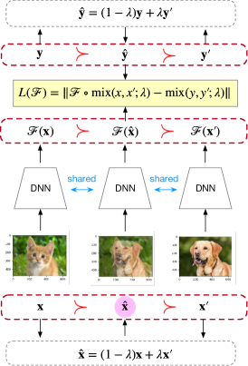
Figure 1: An example of mixup training. Here, a cat and a dog are mixed with a mixing coefficient $\lambda=0.5$. The symbol $\succ$ describes relative ordering along the mixup transformation paths (cat $\succ$ (half-cat+half-dog) $\succ$ dog) in both input and output spaces. Mixup training improves performance by leveraging order relationship along with mixup transformation paths in the hidden space of $\mathcal{F}$.

Data augmentation [4] has been widely used to enhance the performance and generalization capabilities of deep learning models. It enlarges the given training set by applying a variety of transformations to the provided training samples while preserving the original data semantics. Common transformations for image data include random rotation, translation, scaling, and flipping. By introducing these variations, data augmentation helps to mitigate overfitting by providing the model with a more diverse and representative set of examples.

In recent years, mixup [5] has emerged as a powerful data augmentation technique in deep learning. It generates augmented training samples by linearly interpolating pairs of input examples and their corresponding labels. Specifically, given an input-label sample pair $\{({\mathbf{x}},{\mathbf{y}}),({\mathbf{x}}^{\prime},{\mathbf{y}}^{\prime})\}$ from the training set ${\mathcal{D}}$, mixup creates a new sample $(\hat{{\mathbf{x}}},\hat{{\mathbf{y}}})$ via interpolation (Figure 1), where:

$$\hat{{\mathbf{x}}}=\text{mix}({\mathbf{x}},{\mathbf{x}}^{\prime};\lambda),\;\;\hat{{\mathbf{y}}}=\text{mix}({\mathbf{y}},{\mathbf{y}}^{\prime};\lambda),$$ (1)

$\lambda$ is a mixing coefficient drawn from the Beta distribution $Beta(\alpha,\alpha)$ for some $\alpha\in(0,\infty)$, and $\text{mix}(\cdot;\cdot;\lambda)$ is a linear interpolation that mixes the two input arguments based on $\lambda$:

$$\text{mix}({\mathbf{z}},{\mathbf{z}}^{\prime};\lambda)=(1-\lambda){\mathbf{z}}+\lambda{\mathbf{z}}^{\prime}.$$ (2)

Using the implicit order in both the input (denoted ${\mathbf{x}}\succ\hat{{\mathbf{x}}}\succ{\mathbf{x}}^{\prime}$) and output (${\mathbf{y}}\succ\hat{{\mathbf{y}}}\succ{\mathbf{y}}^{\prime}$), the deep network $\mathcal{F}$ is encouraged to behave linearly in-between the training examples $\{({\mathbf{x}},{\mathbf{y}}),({\mathbf{x}}^{\prime},{\mathbf{y}}^{\prime})\}$. In other words, we expect a similar ordering on the network outputs: $\mathcal{F}({\mathbf{x}})\succ\mathcal{F}(\hat{{\mathbf{x}}})\succ\mathcal{F}({\mathbf{x}}^{\prime})$.

Mixup has shown promising results in improving model performance, enhancing generalization, and reducing overfitting [5]. Following its success, a number of variants have been proposed. For instance, manifold mixup [6] explores the application of mixup in the hidden space. FMix [7] incorporates mixing masks of arbitrary shapes, enabling more flexible and diverse sample mixing. Puzzle-mix [8] and co-mixup [9] leverage saliency information to identify informative mixup policies, further enhancing the quality and informativeness of the mixup process. Although mixup and its variants show improved performance, their use of only one single interpolation from each sample pair may limit its augmentation ability.

In this paper, we propose a simple mixup extension called multi-mix, which generates multiple interpolation samples for each sample (and label) pair. For example, from two source samples ${\mathbf{x}}$ and ${\mathbf{x}}^{\prime}$, multi-mix can generate three interpolations $\hat{{\mathbf{x}}}_{1},\hat{{\mathbf{x}}}_{2},\hat{{\mathbf{x}}}_{3}$ with ${\mathbf{x}}\succ\hat{{\mathbf{x}}}_{1}\succ\hat{{\mathbf{x}}}_{2}\succ\hat{{\mathbf{x}}}_{3}\succ{\mathbf{x}}^{\prime}$. By using an ordered sequence of mixup samples, multi-mix can better guide the training process than standard mixup. Moreover, it can be shown theoretically that it also reduces the variance of the stochastic gradient. Extensive experiments are performed to compare the proposed multi-mix with a number of baselines on both synthetic and large-scale data sets. Results demonstrate that multi-mix has superior performance in various aspects including generalization, robustness, and calibration.

The rest of this paper is organized as follows. Section II reviews the related work on the standard mixup and its popular variants. The proposed multi-mix algorithm and corresponding theoretical analysis are presented in Section III. Experimental results are reported in Section IV, and the last section gives some concluding remarks.

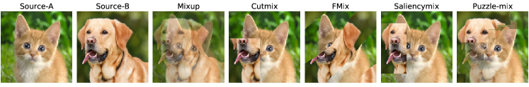
Figure 2: Examples of input mixup and saliency-based mixup techniques.

II Related Work: Mixup and its Variants

Mixup [5] is a recent augmentation approach based on linear interpolation. Due to its simplicity, mixup has attracted much interest in recent years [10, 7, 6, 11, 8, 9, 12]. The various mixup-based methods can be roughly divided into three categories: (i) input mixup, (ii) manifold mixup, and (iii) saliency-based mixup.

Input mixup [5] and its variants [10, 7, 13, 14] augment the data by directly manipulating the input. Besides the standard input mixup, a well-known variant is cutmix [10]. Given two training images ${\mathbf{x}},{\mathbf{x}}^{\prime}$, and the corresponding labels ${\mathbf{y}},{\mathbf{y}}^{\prime}$, cutmix obtains an augmented sample $(\hat{{\mathbf{x}}},\hat{{\mathbf{y}}})$ as:

$$\hat{{\mathbf{x}}} =(\mathbf{1}-\mathbb{I}_{B})\odot{\mathbf{x}}+\mathbb{I}_{B}\odot{\mathbf{x}}^{\prime},\;\;\hat{{\mathbf{y}}}=\text{mix}({\mathbf{y}},{\mathbf{y}}^{\prime};\lambda),$$ (3)

where $\mathbb{I}_{B}$ is a randomly-sampled binary rectangular mask, and $\odot$ is the element-wise product. The mixing ratio $\lambda$ is calculated as the ratio of the area of the rectangular mask and the size of the whole mask $\mathbb{I}_{B}$. FMix [7] further extends cutmix by using binary masks of arbitrary shapes. In Stylemix [13], the content and style information of the input image pairs are leveraged for mixing. Recursivemix [14] explores a recursive mixed-sample learning paradigm in the input space to improve mixup training.

Instead of performing interpolation only at the input, manifold mixup [6] allows interpolation at some hidden layer in a deep network. For each data batch, a layer $s$ (with features $h^{s}(\cdot)$) is first randomly sampled. As in (1), an augmented sample $(\hat{{\mathbf{h}}}^{s},\hat{{\mathbf{y}}})$ is generated by interpolating $(h^{s}({\mathbf{x}}),{\mathbf{y}})$ and $(h^{s}({\mathbf{x}}^{\prime}),{\mathbf{y}}^{\prime})$:

$$\hat{{\mathbf{h}}}^{s} =\text{mix}(h^{s}({\mathbf{x}}),h^{s}({\mathbf{x}}^{\prime});\lambda),\;\;\hat{{\mathbf{y}}}=\text{mix}({\mathbf{y}},{\mathbf{y}}^{\prime};\lambda).$$ (4)

Empirically, this induces smoother boundaries and better generalization. When $s=0$ (the input layer), manifold mixup reduces to standard input mixup. In AlignMixup [12], a matching objective in the hidden space is developed for feature alignment. However, AlignMixup is computationally more expensive as it introduces an additional autoencoder during mixup training.

Saliency-based mixup methods [11, 8, 9, 15, 16, 17] leverage the data’s saliency information to find an informative mixup policy, and have shown performance superior to input and manifold mixup. Instead of using a random selection strategy for mixing, saliencymix [11] selects an informative image patch with a saliency map. Puzzle-mix [8] exploits saliency and local statistics to learn an interpolation strategy for mixing. The augmented sample $(\hat{{\mathbf{x}}},\hat{{\mathbf{y}}})$ is obtained as:

$$\hat{{\mathbf{x}}} = (1-{\mathbf{m}})\odot\Pi_{0}^{\top}s({\mathbf{x}})+{\mathbf{m}}\odot\Pi_{1}^{\top}s({\mathbf{x}}^{\prime}),$$ (5)

$$\hat{{\mathbf{y}}} = \text{mix}({\mathbf{y}},{\mathbf{y}}^{\prime};\hat{\lambda}),$$

where $s(\cdot)$ measures the saliency, and $\Pi_{0}$ and $\Pi_{1}$ are learnable transport plans for the inputs. The mask ${\mathbf{m}}$, with elements $m_{i}$’s in $[0,1]$, is represented as a vector. Each $m_{i}$ is discretized to $d+1$ values: $\{\frac{t}{d}\;|\;t=0,1,\dots,d\}$. Given a $\lambda$ that is randomly sampled from a Beta distribution, $m_{i}$ is generated from the mixing prior $p\left(m_{i}=\frac{t}{d}\right)=\binom{d}{t}\lambda^{t}(1-\lambda)^{d-t}$. Consequently, the mixing ratio $\hat{\lambda}$ for label mixing is set as $\frac{1}{n}\sum^{n}_{i=1}m_{i}$. Intuitively, the mask ${\mathbf{m}}$ and transport plans try to maximize the saliency of the revealed portion of the image. Co-mixup [9] is an extension of puzzle-mix. Instead of mixing only a random pair of input samples, co-mixup generates a batch of mixup samples by accumulating many salient regions from multiple input samples.

Figure 2 shows examples generated by input mixup and some of its variants. As can be seen, input mixup simply overlaps the two source images, which weakens the original information of the object. Cutmix and FMix can well preserve the clarity of the original object. However, the most informative parts may not be included in the mixing result. Saliencymix well covers the important area, but may have sharp borders in the resulting image. The image by puzzle-mix covers the most informative parts and also has smoother borders. This suggests that choosing puzzle-mix as the basic mixup operation in multi-mix is more effective in introducing additional information about the mixup transformation path, thereby aiding in the regularization of network training.

Figure 3: Examples interpolations ($\hat{h}^{0}_{1},\hat{h}^{0}_{2},\hat{h}^{0}_{3},\hat{h}^{0}_{4}$) generated by input mixup (top), cutmix (middle), and puzzle-mix (bottom).

III Multi-Mix: Mixup with Multiple Interpolations

Existing mixup methods generate only one single interpolation for each sample pair. To introduce more mixup information on the mixup transformation path for regularizing the network, we propose multi-mix, which generates mixup sample pairs $\{(\hat{{\mathbf{h}}}_{k}^{s},\hat{{\mathbf{h}}}_{k}^{s})\}_{k=1}^{K}$ with $K>1$ interpolations.

Section III-A describes how this can be extended to multiple interpolations. Section III-B provides theoretical analysis on the effect of using multiple interpolations on gradient variance. Section III-C discusses related methods that also increase the number of mixup samples in each batch.

III-A Generating Multiple Interpolations

In the following, we focus on multi-mix extensions of input mixup, manifold mixup, cutmix and puzzle-mix. Extensions for other mixup variants can be developed analogously.

III-A1 Extending Input Mixup and Manifold Mixup

The multi-mix extensions for input mixup and manifold mixup are straightforward. Given a deep network and a pair of random samples ${\mathbf{x}}$ and ${\mathbf{x}}^{\prime}$, the $K$ interpolations $\{(\hat{{\mathbf{h}}}_{k}^{s},\hat{{\mathbf{y}}}_{k})\}_{k=1}^{K}$ can be generated from input mixup or manifold mixup as:

$$\hat{{\mathbf{h}}}_{k}^{s}=\text{mix}(h^{s}({\mathbf{x}}),h^{s}({\mathbf{x}}^{\prime});\lambda_{k}),\;\hat{{\mathbf{y}}}_{k}=\text{mix}({\mathbf{y}},{\mathbf{y}}^{\prime};\lambda_{k}),$$ (6)

where $s$ is the layer index, and $h^{s}({\mathbf{x}}),h^{s}({\mathbf{x}}^{\prime})$ are the layer-$s$ outputs of ${\mathbf{x}},{\mathbf{x}}^{\prime}$, respectively. For input mixup, $s=0$; whereas for manifold mixup, $s>0$. The $\lambda_{i}$’s satisfy $0<\lambda_{1}<\dots<\lambda_{K}<1$, and are randomly sampled from the same Beta distribution.

III-A2 Extending Cutmix

For cutmix with $K$ interpolations, we need to generate $K$ boxes indicating the $K$ regions of ${\mathbf{x}}$ that are cropped and replaced by the corresponding regions in ${\mathbf{x}}^{\prime}$. We first sample the center that is shared by the $K$ boxes. Let its coordinates be $(r^{x},r^{y})$, where $r^{x}\sim\mathrm{uniform}(0,W)$, $r^{y}\sim\mathrm{uniform}(0,H)$, and $W,H$ are the image’s width and height, respectively. The width and height of the $k$th box are given by $r^{w}_{k}=W\sqrt{{\lambda}_{k}}$ and $r^{h}_{k}=H\sqrt{{\lambda}_{k}}$, respectively, where ${\lambda}_{k}$ is randomly sampled from a Beta distribution.

III-A3 Extending Puzzle-mix

For puzzle-mix with $K$ interpolations, we generate $K$ masks (${\mathbf{m}}_{k}$’s) in (5) by using $K$ mask-mixing priors $\{p_{k}(m_{i})\}_{k=1,2,\dots,K}$. Each $p_{k}(m_{i})$ is parameterized by a $\lambda_{k}$ that is also randomly sampled from a shared Beta distribution.

Figure 3 shows examples generated by the multi-mix extensions of input mixup, cutmix and puzzle-mix on a pair of example images. As can be seen, the generated multiple interpolations show a continuous transformation from one image (cat) to another (dog). For example, consider the multi-mix extension of cutmix (second row). When the cropping box is small, the augmented sample is closer to the cat (left). When the cropping box becomes larger, the sample becomes more like the dog (right).

III-B Variance Reduction with Multi-Mix

Theoretical analysis shows that a small variance in the stochastic gradients can lead to faster convergence [18]. In this section, we theoretically show that multi-mix can reduce this gradient variance.

Instead of only minimizing the loss on the original data samples, mixup and its variants generate artificial samples during training and can be regarded as optimizing the following mixup loss [19, 20]:

$${\mathcal{L}}_{\texttt{mixup}}=\mathop{\mathbb{E}}_{\lambda\sim Beta(\alpha,\alpha)}\mathop{\mathbb{E}}_{({\mathbf{x}},{\mathbf{y}}),({\mathbf{x}}^{\prime},{\mathbf{y}}^{\prime})\in{{\mathcal{D}}}}\mathcal{L}(({\mathbf{x}},{\mathbf{y}}),({\mathbf{x}}^{\prime},{\mathbf{y}}^{\prime}),\lambda),$$

where ${\mathcal{D}}$ is the training set, and $\mathcal{L}(({\mathbf{x}},{\mathbf{y}}),({\mathbf{x}}^{\prime},{\mathbf{y}}^{\prime}),\lambda)$ is the loss on a mixup sample generated from the sample pair $\{({\mathbf{x}},{\mathbf{y}}),({\mathbf{x}}^{\prime},{\mathbf{y}}^{\prime})\}$ with mixup weight $\lambda$. Empirically, for mixup (or its variants) with single interpolation, ${\mathcal{L}}_{\texttt{mixup}}$ is approximated as $\frac{1}{|{{\mathcal{D}}}|}\sum_{({\mathbf{x}},{\mathbf{y}}),({\mathbf{x}}^{\prime},{\mathbf{y}}^{\prime})\in{{\mathcal{D}}}}\mathcal{L}(({\mathbf{x}},{\mathbf{y}}),({\mathbf{x}}^{\prime},{\mathbf{y}}^{\prime}),\lambda)$.

With the proposed multi-mix, ${\mathcal{L}}_{\texttt{mixup}}$ is approximated as

$${\mathcal{L}}_{\texttt{multi-mix}}=\frac{1}{K|{{\mathcal{D}}}|}\sum_{({\mathbf{x}},{\mathbf{y}}),({\mathbf{x}}^{\prime},{\mathbf{y}}^{\prime})\in{{\mathcal{D}}}}\sum_{k=1}^{K}\mathcal{L}(({\mathbf{x}},{\mathbf{y}}),({\mathbf{x}}^{\prime},{\mathbf{y}}^{\prime}),\lambda_{k}).$$

In a particular training iteration, a batch ${\mathcal{B}}$ of $B$ samples from ${{\mathcal{D}}}$ are sampled, and a total of $KB$ mixup samples are generated. For multi-mix, the gradient of the mixup loss on ${\mathcal{B}}$ is:

$$\tilde{{\mathbf{g}}}=\frac{1}{KB}\sum_{({\mathbf{x}},{\mathbf{y}}),({\mathbf{x}}^{\prime},{\mathbf{y}}^{\prime})\in{\mathcal{B}}}\sum_{k=1}^{K}{\mathbf{g}}(({\mathbf{x}},{\mathbf{y}}),({\mathbf{x}}^{\prime},{\mathbf{y}}^{\prime}),\lambda_{k}),$$ (7)

where ${\mathbf{g}}(({\mathbf{x}},{\mathbf{y}}),({\mathbf{x}}^{\prime},{\mathbf{y}}^{\prime}),\lambda_{k})=\nabla\mathcal{L}(({\mathbf{x}},{\mathbf{y}}),({\mathbf{x}}^{\prime},{\mathbf{y}}^{\prime}),\lambda_{k})$ is the loss gradient on a mixup sample generated from $\{({\mathbf{x}},{\mathbf{y}})$, $({\mathbf{x}}^{\prime},{\mathbf{y}}^{\prime})\}$ with mixup weight $\lambda_{k}$. Obviously, we have $\mathbb{E}[\tilde{{\mathbf{g}}}]=\nabla{\mathcal{L}}_{\texttt{mixup}}$. Define

$$\mathrm{Var}[\tilde{{\mathbf{g}}}]=\mathbb{E}[\|\tilde{{\mathbf{g}}}-\mathbb{E}[\tilde{{\mathbf{g}}}]\|^{2}]=\mathbb{E}[\|\tilde{{\mathbf{g}}}\|^{2}]-(\mathbb{E}[\|\tilde{{\mathbf{g}}}\|])^{2}$$ (8)

as the variance of $\tilde{{\mathbf{g}}}$ w.r.t. the data and mixup weights of $\tilde{{\mathbf{g}}}$. The following Proposition shows that multi-mix reduces the gradient’s variance.

Proposition III.1.

$\mathrm{Var}[\tilde{{\mathbf{g}}}]$ decreases with $K$.

Proof is in Appendix A-A. While Proposition III.1 suggests the use of a large $K$, the number of gradient computations also grows with $K$. Moreover, as will be seen in Section IV-I, empirically the performance saturates when $K$ is sufficiently large.

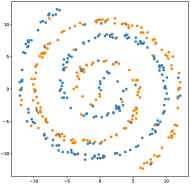
(a) Noisy Spiral.

(b) no mixup (90.67%).

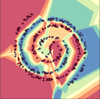
(c) Manifold-mix (94.17%).

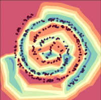
(d) Multi-mix (97.50%).

Figure 4: The noisy spiral data and decision boundaries learned without mixup, with manifold mixup, and manifold mixup with multiple interpolations. Values in brackets are the top-1 test accuracies obtained.

III-C Discussion

The proposed multi-mix introduces more (i.e., a total of $KB$) mixup samples in each batch to help network training. In this section, we discuss related methods that also increase the number of mixup samples in each batch. Note that they do not optimize the networks by introducing more mixup transformation path information as in multi-mix. As will be empirically demonstrated in Section IV, this mixup transformation path is helpful in improving generalization, robustness against data corruption, transferability, and calibration.

III-C1 Large-batch Training

A simple approach (often called large-batch training [21]) is to just use a larger batch size, without mixup (or its variants). However, as discussed in [21], the model’s generalization ability may be degraded in practice. This will also be empirically verified in Section IV-B2.

III-C2 Large-batch Mixup

Alternatively, one can simply use standard mixup (or its variants), but with $KB$ mixup samples. To differentiate this from mixup (using only $B$ mixup samples), we will refer to this as “large-batch mixup” in the sequel. Its loss gradient is

$$\tilde{{\mathbf{g}}}^{\prime}=\frac{1}{KB}\sum_{({\mathbf{x}},{\mathbf{y}}),({\mathbf{x}}^{\prime},{\mathbf{y}}^{\prime})\in{\mathcal{B}}}{\mathbf{g}}(({\mathbf{x}},{\mathbf{y}}),({\mathbf{x}}^{\prime},{\mathbf{y}}^{\prime}),\lambda),$$ (9)

where a single $\lambda$ is sampled from $Beta(\alpha,\alpha)$ and used on all sample pairs in the batch. Note that both (7) and (9) involve $KB$ gradient computations, and thus have the same computational cost in one batch update.

Let $\mathrm{Var}[\tilde{{\mathbf{g}}}^{\prime}]=\mathbb{E}[\|\tilde{{\mathbf{g}}}^{\prime}-\mathbb{E}[\tilde{{\mathbf{g}}}^{\prime}]\|]$ be the variance of the stochastic gradient $\tilde{{\mathbf{g}}}^{\prime}$ w.r.t. the data and mixup weights. The following Proposition shows that with the same computational cost (i.e., $KB$ gradient computations), multi-mix has a smaller variance than large-batch mixup when $B$ is large enough. Proof is in Appendix A-B.

Proposition III.2.

For any $K>1$, $\mathrm{Var}[\tilde{{\mathbf{g}}}]\leq\mathrm{Var}[\tilde{{\mathbf{g}}}^{\prime}]$ when

$$B\geq\frac{\mathrm{Var}_{({\mathbf{x}},{\mathbf{y}}),({\mathbf{x}}^{\prime},{\mathbf{y}}^{\prime})}\mathbb{E}_{\lambda_{k}\sim Beta(\alpha,\alpha)}[{\mathbf{g}}(({\mathbf{x}},{\mathbf{y}}),({\mathbf{x}}^{\prime},{\mathbf{y}}^{\prime}),\lambda_{k})]}{\mathrm{Var}_{\lambda_{k}\sim Beta(\alpha,\alpha)}\mathbb{E}_{({\mathbf{x}},{\mathbf{y}}),({\mathbf{x}}^{\prime},{\mathbf{y}}^{\prime})}[{\mathbf{g}}(({\mathbf{x}},{\mathbf{y}}),({\mathbf{x}}^{\prime},{\mathbf{y}}^{\prime}),\lambda_{k})]}.$$

With a smaller gradient variance, multi-mix converges faster than large-batch mixup. It also has better generalization performance, as will be empirically verified in Section IV-B2. Thus, with the same computation cost, using more interpolations is preferred over the use of more data sample pairs.

III-C3 Batch Augmentation

Multi-mix is also similar to batch augmentation [22], which replicates samples in the same batch with different data augmentations (e.g., random cropping and horizontal flipping). To enhance batch augmentation, mixup can also be used to further enlarge the dataset. However, while batch augmentation focuses on replicating each sample by different transformations, multi-mix generates multiple mixup samples from each sample pair.

IV Experiments

In this section, we perform extensive evaluation of the proposed multi-mix on various tasks, including synthetic image classification (Section IV-A), real-world image classification (Sections IV-B and IV-C), weakly-supervised object localization (Section IV-D), corruption robustness (Section IV-E), transfer learning (Section IV-F), speech recognition (Section IV-G), and calibration analysis (Section IV-H). Section IV-I presents some ablation studies.

	CIFAR-100			Tiny-ImageNet
	PreActResNet18	WRN16-8	ResNeXt29-4-24	PreActResNet18
no mixup	23.53 $\pm$ 0.39	21.93 $\pm$ 0.52	21.84 $\pm$ 0.16	43.54 $\pm$ 0.13
Input mixup	22.49 $\pm$ 0.21	20.18 $\pm$ 0.51	21.78 $\pm$ 0.09	43.35 $\pm$ 0.12
Manifold mixup	21.62 $\pm$ 0.29	20.49 $\pm$ 0.46	21.45 $\pm$ 0.12	41.21 $\pm$ 0.10
Cutout	21.12 $\pm$ 0.38	19.19 $\pm$ 0.39	20.86 $\pm$ 0.13	40.52 $\pm$ 0.15
Cutmix	21.29 $\pm$ 0.26	20.14 $\pm$ 0.50	20.92 $\pm$ 0.10	43.11 $\pm$ 0.12
FMix	21.52 $\pm$ 0.24	19.75 $\pm$ 0.49	21.87 $\pm$ 0.10	42.38 $\pm$ 0.15
Co-mixup	19.89 $\pm$ 0.28	19.24 $\pm$ 0.31	19.43 $\pm$ 0.08	35.94 $\pm$ 0.11
Puzzle-mix	20.61 $\pm$ 0.29	19.27 $\pm$ 0.32	19.74 $\pm$ 0.09	36.79 $\pm$ 0.07
Label-smoothing	23.09 $\pm$ 0.34	21.45 $\pm$ 0.44	20.66 $\pm$ 0.12	43.04 $\pm$ 0.12
Multi-mix (with Puzzle-mix)	19.19 $\pm$ 0.27	18.52 $\pm$ 0.32	18.23 $\pm$ 0.06	34.84 $\pm$ 0.08

TABLE I: Test errors (%) on CIFAR-100 and TinyImagenet. The best results are in bold. The second-best results are underlined. The improvements are statistically significant based on the pairwise t-test at 95% significance level.

IV-A Synthetic Data Classification

Inspired by [6], this experiment uses the synthetic data set Spiral to study the decision boundary learned by the proposed multi-mix. We generate 1,000 samples. 40% of them are used for training, and the rest for testing. To evaluate the method’s robustness, 20% of the training labels are randomly flipped (Figure 4(a)). We consider manifold mixup with $K=1$ and with $K=5$ interpolations. A feed-forward network with eight hidden layers (six units in each layer) and a linear output layer is used. The interpolation is performed in a shallow layer (randomly selected from layers 1 and 2). The network is $\ell_{2}$-regularized and optimized by the Adam optimizer [23], with a learning rate of 0.01. The number of epochs is 3,000, and the batch size is 256.

Figure 4 shows the decision boundaries learned without mixup (Figure 4(b)), with manifold mixup (Figure 4(c)), and with multi-mix extension of manifold mixup (Figure 4(d)). As can be seen, using multiple interpolations enhances manifold mixup, induces a much smoother decision boundary, and improves testing accuracy.

IV-B Classification on CIFAR-100 and TinyImagenet

In this experiment, we use two standard image classification benchmark datasets: CIFAR-100 [24] and Tiny-ImageNet [25]. CIFAR-100 has 100 classes and contains 60,000 32$\times$ 32 color images. The number of training images and test images are 50,000 and 10,000, respectively. Tiny-ImageNet contains 200 classes of $64\times 64$ images. Each class has 500 training images and 50 test images.

IV-B1 Comparison with Various Mixup Variants and Label Smoothing

We use three deep networks (PreActResNet18 [26], WRN16-8, [27] and ResNeXt29-4-24 [28]) for CIFAR-100. Following [9], we use the SGD optimizer with an initial learning rate of 0.2, which is decayed by a factor of 0.1 at epochs 100 and 200. The total number of training epochs is 300. For Tiny-ImageNet, we follow the setting in [8] and use PreActResNet18 with 1,200 training epochs. We use the SGD optimizer with an initial learning rate of 0.2, which is decayed by a factor of 0.1 at epochs 600 and 900. The batch size is 100. To allow parallelism, we use PyTorch’s multi-process data loading technique [29] (with 8 loader worker processes). The experiment is run on a single NVIDIA V6000 GPU.

As discussed in Section III-A, puzzle-mix can generate more informative mixup images. Thus, we apply the proposed multi-mix (with $K=5$) on puzzle-mix. The use of multi-mix on other mixup variants is shown in Section IV-I.

The proposed method is compared with the vanilla classifier (having no mixup) and various mixup variants including (i) input mixup [5], (ii) manifold mixup [6], (iii) cutout [30], (iv) cutmix [10], (v) FMix [7], (vi) co-mixup [9] and (vii) puzzle-mix [8]. Besides, we follow [5] and include (viii) label smoothing [31], which alleviates over-fitting by introducing label noise.

For performance evaluation, as in [8, 9], we use the classification error on the test set. The experiment is repeated three times with different random seeds, and then the average performance is reported.

Table I shows the test errors obtained by the various methods. As can be seen, multi-mix outperforms all the other mixup variants. On CIFAR-100, it achieves improvements of 1.42%, 0.75% and 2.29% over standard puzzle-mix on networks PreActResNet18, WRN16-8, and ResNeXt29-4-24, respectively. It also improves standard puzzle-mix on TinyImagenet by 1.68%. This demonstrates that leveraging multiple interpolations can improve generalization performance.

IV-B2 Comparison with Large-Batch Training, Large-Batch Mixup, and Batch Augmentation

In this experiment, using the same setup with puzzle-mix as in Section IV-B1, we compare with the baselines discussed in Section III-C (namely, (i) batch augmentation [22] and (ii) its variant with mixup; (iii) large-batch training [21], and (iv) large-batch mixup).

For batch augmentation (and its mixup variant), we keep the original batch size of 100. As $K=5$ interpolations are used in multi-mix, we run each label-preserving augmentation (random crop, flipping, and rotation) 5 times for every sample in the batch. The augmented batch size is thus the same as that of multi-mix. Similarly, the batch size for large-batch training and large-batch mixup is $100\times 5=500$.

	test error (%)
large-batch training	33.45 $\pm$ 0.11
large-batch mixup	26.54 $\pm$ 0.07
batch augmentation	20.91 $\pm$ 0.11
batch augmentation with mixup	19.41 $\pm$ 0.08
multi-mix	18.23 $\pm$ 0.06

TABLE II: Test errors (%) of various multiple-augmentation strategies on CIFAR-100.

Table II shows the testing errors on CIFAR-100 using the ResNeXt29-4-24 network. As can be seen, the performance of large-batch training is poor, as it tends to converge to sharp minima of the training loss [21]. Large-batch mixup alleviates the issue of sharp minima and brings some improvements. While batch augmentation and its mixup variant lead to improved generalization performance, multi-mix improves the performance further by a larger margin. This can be explained by the fact that multi-mix can introduce more information in the mixup transformation path in one gradient update. Although large-batch mixup and batch augmentation also produce more augmented samples for gradient update, their generated samples do not include mixup transformation path information as much as in multi-mix.

IV-C Large-Scale ImageNet-1K Classification

In this experiment, we perform large-scale image classification using the ImageNet data [32]. It contains 1.2 million training images and 50,000 validation images from 1,000 classes. For fair comparison, we follow the training protocol in [9] and report the validation error.

We use the ResNet-50 [33], which is trained for a total of 100 epochs. As in [9], these 100 epochs are divided into three stages. From epochs 0-15, input images are resized to 160$\times$160. The initial learning rate is 0.5, and is increased linearly to 1.0 for the first 8 epochs and then decreased linearly to 0.125 until epoch 15. From epochs 16-40, images are resized to 352$\times$352. The learning rate is initially set to 0.2, and decreased linearly to 0.02 at epoch 40. Finally, for the remaining epochs, the image size is still 352$\times$352, but the learning rate is decayed by 0.1 at epochs 65 and 90. SGD is used throughout. Moreover, only basic data augmentation strategies, including random crop and random horizon flip, are used. The proposed multi-mix is compared with no mixup, input mixup, manifold mixup, cutmix, co-mixup and puzzle-mix.

	validation error (%)
no mixup	24.03
Input mixup	22.97
Manifold mixup	23.30
Cutout	24.10
Cutmix	22.92
FMix	23.96
Co-mixup	22.39
Puzzle-mix	22.54
Label smoothing	23.44
Multi-mix (with Puzzle-mix)	22.29

TABLE III: Validation error (%) on ImageNet-1K. The best results are in bold. The second-best results are underlined. Results of the baselines are from [9].

Table III shows the validation errors. Co-mixup has the lowest error of 22.39% among all baselines, and outperforms puzzle-mix by 0.15%. However, the multi-mix extension of puzzle-mix improves co-mixup by 0.10%.

IV-D Weakly-Supervised Object Localization

In this experiment, we perform weakly-supervised object localization (WSOL) [34], which uses image-level labels to identify the part containing the target object in an image from ImageNet without any pixel-level supervision. Following [35], we use the WSOL method of CAM [36], which uses a pre-trained classifier to obtain the target object’s bounding box. Here, we use the networks trained on ImageNet in Section IV-C as the pre-trained classifier.

For performance evaluation, we use the localization accuracy [9] (also called correct localization metric [37]), which is the percentage of images that are correctly localized. The predicted bounding box is considered correct if the intersection over union (IoU) [38] value between the predicted bounding box and one of the ground-truth bounding boxes is higher than 0.25. Intuitively, if the network has learned informative representations from the data, it should perform better on WSOL.

Results are shown in Table IV. Again, the proposed method outperforms all the baselines. This shows leveraging multi-mix helps to learn informative representations in deep networks.

	localization accuracy (%)
no mixup	54.36
Input mixup	55.07
Manifold mixup	54.86
Cutout	54.24
Cutmix	54.91
FMix	54.57
Co-mixup	55.32
Puzzle-mix	55.22
Label smoothing	54.37
Multi-mix (with Puzzle-mix)	55.43

TABLE IV: Localization accuracy (%) in WSOL task. The best results are in bold. The second-best results are underlined.

	random replacement	Gaussian noise
no mixup	41.63	29.22
Input mixup	39.41	26.29
Manifold mixup	39.72	26.79
Cutout	41.75	29.13
Cutmix	46.20	27.13
FMix	41.42	28.58
Co-mixup	38.77	25.89
Puzzle-mix	39.23	26.11
Label smoothing	39.55	27.77
Multi-mix (with Puzzle-mix)	39.01	25.53

TABLE V: Validation errors (%) on background-corrupted ImageNet datasets. The best results are in bold. The second-best results are underlined.

	fine-tuning steps
	1	2	3	4	5	6	7	8	9	10
no mixup	28.22	59.67	76.59	84.48	90.81	92.56	92.89	93.93	93.85	94.43
Input mixup	33.30	64.78	75.90	84.42	92.41	93.62	94.12	94.71	94.99	95.09
Manifold mixup	35.07	67.59	77.96	82.70	91.71	93.36	94.12	94.62	94.83	95.22
Cutout	30.70	64.34	77.99	82.91	90.95	92.59	93.45	93.97	94.12	94.49
Cutmix	39.59	67.99	80.92	86.47	92.93	94.04	94.98	95.21	95.44	95.71
FMix	28.13	58.20	75.34	82.80	90.13	91.96	93.10	93.52	93.71	94.27
Co-mixup	40.78	67.89	82.56	87.20	92.65	94.09	94.90	95.19	95.43	95.81
Puzzle-mix	39.37	70.16	82.69	87.60	93.39	94.45	94.92	95.41	95.57	95.82
Label-smoothing	38.64	64.40	79.31	85.48	91.86	93.37	94.17	94.68	95.01	95.21
Multi-mix (with Puzzle-mix)	45.14	74.72	84.48	88.36	94.10	95.24	95.94	96.08	96.23	96.49

TABLE VI: Localization accuracy (in %) with different numbers of fine-tuning steps on CUB 200-2011. The best results are in bold. The second-best results are underlined.

IV-E Robustness to Corruption

In this section, we evaluate the robustness to images with corrupted background of the various trained ResNet-50 models in Section IV-C. As in [9], the ImageNet validation set images are used. Their backgrounds are corrupted by either (i) random replacement with another image from the validation set, or (ii) addition of Gaussian noise from $\mathcal{N}(0,0.1^{2})$.

Table V shows the validation errors. The proposed puzzle-mix with multiple interpolations shows good robustness against both kinds of background corruption. For random replacement, the use of multiple interpolations improves puzzle-mix, and is competitive with co-mixup. For Gaussian-noise corruption, the proposed method outperforms all mixup baselines. This supports the intuition that multiple interpolations help to induce more robust representations.

IV-F Transfer Learning to Fine-Grained CUB 200-2011

In this experiment, we study the transferability of the various ResNet-50 models trained in Section IV-C. Each model is transferred to the task of object localization on the fine-grained CUB 200-2011 dataset [39], by fine-tuning the last ResNet block and fully-connected layer for a maximum of 10 epochs (using the Adam optimizer with a learning rate of 0.0001). We use the localization accuracy for performance evaluation. The binarization threshold is set to 0.75 as in [40].

Table VI shows the localization accuracies when the number of fine-tuning steps is varied from 1 to 10. Note that using more fine-tuning steps improves performance. As can be seen, the network pretrained using multiple interpolations takes fewer fine-tuning steps and has better localization performance than networks pretrained by the other mixup methods.

Figure 5 shows examples produced by the networks pretrained with different mixup methods with only one fine-tuning step. As can be seen, the predicted bounding box by the proposed method localizes the target object with higher accuracy. This supports that networks augmented by the proposed method are more informative.

	test error (%)
no mixup	4.84
Input mixup	3.91
Manifold mixup	3.67
Cutout	3.76
Cutmix	4.36
FMix	4.10
Co-mixup	3.54
Puzzle-mix	3.70
Label smoothing	4.72
Multi-mix (with Puzzle-mix)	3.41

TABLE VII: Test error (%) on the Google commands dataset. The best results are in bold. The second-best results are underlined.

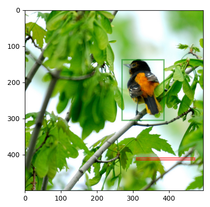
(a) no mixup.

(b) Input mixup.

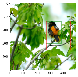
(c) Manifold mixup.

(d) Cutmix.

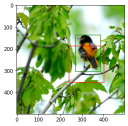
(e) Cutout.

(f) FMix.

(g) Co-mixup.

(h) Puzzle-mix.

(i) Label-smoothing.

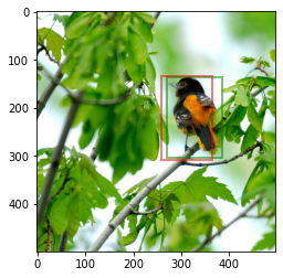
(j) Multi-mix (with Puzzle-mix) .

Figure 5: Example localization results on CUB 200-2011 from networks pretrained with different mixup methods. Red: Predicted bounding box; Green: Ground-truth bounding box.

IV-G Classification on Speech Data

In this experiment, we perform speech classification on the Google commands dataset [41]. This includes 65,000 utterances from 30 categories (e.g., “On”, “Off”, “Stop”, and “Go”). Following [5], the raw waveform utterances are preprocessed by short-time Fourier transform [42] to extract normalized spectrograms. We then use the VGG-11 network [43] and perform various mixup methods at the spectrogram level. The network is trained by SGD for 30 epochs. The initial learning rate is $0.003$ and is decayed by a factor of 10 every 10 epochs. This dataset has a standard training/validation/test split. Following [9], we select the best model based on the validation error and report the corresponding test error.

Table VII shows the test errors. As can be seen, the proposed method again outperforms all the baselines.

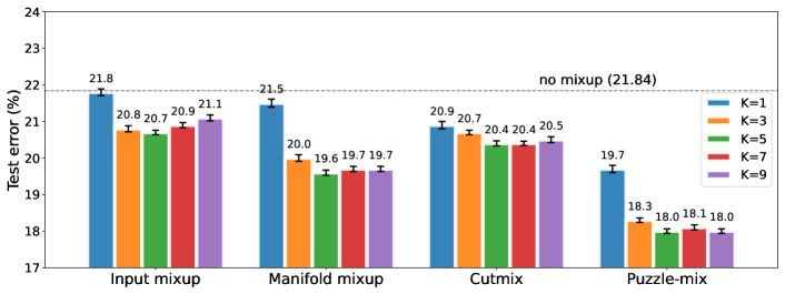
Figure 6: Test errors of the proposed multi-mix extensions on various mixup strategies with different $K$’s. For comparison, the performance with no mixup is shown by the dotted line.

IV-H Calibration Analysis

Deep networks trained with mixup are often better calibrated than models trained without mixup [44]. A well-calibrated model is not over-confident and produces softmax scores that are close to the actual likelihoods of correctness. In this experiment, we study the ResNet-50 models trained on the ImageNet in Section IV-C.

Performance evaluation is based on the popularly-used expected calibration error (ECE) [45, 9]. Specifically, predictions from all test samples are grouped into $M$ bins (each of size $1/M$). Following [9], we used $M=10$. Let $B_{m}$ be the set of samples whose largest softmax scores fall in the interval $I_{m}=\left(\frac{m-1}{M},\frac{m}{M}\right]$. The average accuracy of bin $B_{m}$ is

$$\operatorname{acc}(B_{m})=\frac{1}{|B_{m}|}\sum_{i\in B_{m}}\mathbf{1}(\hat{y}_{i}=y_{i}),$$

where $\hat{y}_{i}$ and $y_{i}$ are the predicted and true class labels for sample $i$, respectively. Similarly, the average confidence of bin $B_{m}$ is defined as:

$$\operatorname{conf}(B_{m})=\frac{1}{|B_{m}|}\sum_{i\in B_{m}}\hat{p}_{i},$$

where $\hat{p}_{i}$ is the logistic output of sample $i$. ECE is then defined as:

$$\mathrm{ECE}=\sum_{m=1}^{M}\frac{|B_{m}|}{n}|\operatorname{acc}(B_{m})-\operatorname{conf}(B_{m})|.$$

A well-calibrated model should have a small ECE.

	ECE (%)
no mixup	5.93
Input mixup	1.18
Manifold mixup	1.70
Cutout	5.72
Cutmix	4.31
FMix	5.89
Co-mixup	2.17
Puzzle-mix	2.06
Label smoothing	5.39
Multi-mix (with Puzzle-mix)	1.46

TABLE VIII: ECE (%) of the ResNet-50 models trained on ImageNet. The best results are in bold. The second-best results are underlined.

Table VIII shows the ECE results. As can be seen, the network trained with the proposed method is better calibrated than most baselines (except input mixup). While input mixup leads to the lowest ECE, its classification error on the same task is high (see Table III). Thus, the proposed method achieves very competitive ECE performance while having the lowest classification error.

Figure 7: Percentage increase in per-epoch training time with $K$ (linear scaling is shown in orange).

IV-I Ablation Study: Effect of $K$

In this experiment, we study the effect of $K$, the number of interpolations. We compare the training time of puzzle-mix (with $K=1$ interpolation) and its multi-mix version (with $K=3,5,7,9$ interpolations) on CIFAR100. We use the setup in Section IV-B. Besides puzzle-mix, we also study the multi-mix extensions of input mixup, manifold mixup and cutmix. The network used is ResNeXt29-4-24, which is trained in the same manner as in section IV-B. The experiment is repeated three times, and both the mean test error and its standard deviation are reported.

Figure 6 shows the test error with different $K$’s. As can be seen, the use of multiple interpolations benefits all mixup variants to different extents. Improvements in input mixup and cutmix are relatively small. This may be due to that their mixing results may lose some object information in the source images, and cutmix causes sharp mixing-box boundaries (see Fig 2). For puzzle-mix, the performance improves with larger $K$. However, a large $K$ is not necessary. In practice, we set $K$ to 5.

Figure 7 shows the relative increase in per-epoch training time of multi-mix (with puzzle-mix) over standard puzzle-mix with different values of $K$. As can be seen, the training time increases with $K$, though sublinearly because of the use of parallelism.

Finally, we provide empirical evidence for the reduction in gradient variance as discussed in Section III-B. Note that directly computing the gradient variance using (8) can be difficult, as it requires computing both $\mathbb{E}[\|\tilde{{\mathbf{g}}}\|^{2}]$ and $\mathbb{E}[\tilde{{\mathbf{g}}}]$. However, for any $K$, we have $\mathbb{E}[\tilde{{\mathbf{g}}}]=\nabla{\mathcal{L}}_{{mixup}}$ (section III-B) which does not depend on $K$. Hence, a larger $\mathbb{E}[\|\tilde{{\mathbf{g}}}\|^{2}]$ indicates a larger gradient variance $\mathrm{Var}[\tilde{{\mathbf{g}}}]$. As such, following [22], we use the expectation of the squared norm $\|\tilde{{\mathbf{g}}}\|^{2}$ as a surrogate to compare $\mathrm{Var}[\tilde{{\mathbf{g}}}]$. We estimate the gradient norm in each batch and average over the whole epoch.

Figure 8 shows the squared $\ell_{2}$-norm of the stochastic gradient with the number of training epochs. As can be seen, the use of a large $K$ reduces the gradient norm, thus supporting the theoretical analysis in Proposition III.1.

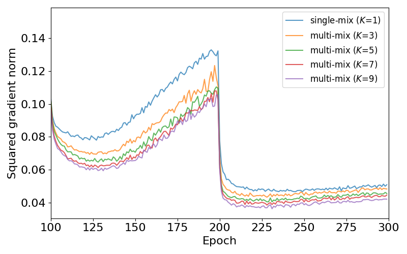
Figure 8: $\ell_{2}$-norm of gradients versus number of training epochs on CIFAR-100. Note that the drop at epoch 200 in Figure 8 is a result of the learning rate decay by a factor of 0.1.

V Conclusion

In this work, we propose a simple yet powerful extension of mixup and its variants with the use of multiple interpolations. Theoretical analysis shows that it can reduce the variance of stochastic gradients, leading to better optimization. Extensive experiments demonstrate that this can improve generalization, induce smoother decision boundaries, and learn more informative representations. Moreover, the obtained network is more robust against data corruption, more transferable, and better calibrated. Hence, this leveraging of mixup order relationships offers an easy and effective tool to improve the mixup family.

Appendix A Proofs

A-A Proof of Proposition III.1

Let the variance of ${\mathbf{g}}(({\mathbf{x}},{\mathbf{y}}),({\mathbf{x}}^{\prime},{\mathbf{y}}^{\prime}),\lambda)$ be

$$\mathrm{Var}[{\mathbf{g}}(({\mathbf{x}},{\mathbf{y}}),({\mathbf{x}}^{\prime},{\mathbf{y}}^{\prime}),\lambda)]=\mathbb{E}[\|{\mathbf{g}}(({\mathbf{x}},{\mathbf{y}}),({\mathbf{x}}^{\prime},{\mathbf{y}}^{\prime}),\lambda)-{\mathbf{g}}\|^{2}],$$

where

$${\mathbf{g}}=\mathbb{E}_{({\mathbf{x}},{\mathbf{y}}),({\mathbf{x}}^{\prime},{\mathbf{y}}^{\prime})}\mathbb{E}_{\lambda_{k}}[{\mathbf{g}}(({\mathbf{x}},{\mathbf{y}}),({\mathbf{x}}^{\prime},{\mathbf{y}}^{\prime}),\lambda_{k})].$$

For simplicity of notations, $\lambda_{k}$ is always sampled from $Beta(\alpha,\alpha)$ in the sequel. Since we have two sources of stochasticity (sample pairs and $\lambda$), and they are independent of each other, we can decouple the variance as:

$$\mathrm{Var}[{\mathbf{g}}(({\mathbf{x}},{\mathbf{y}}),({\mathbf{x}}^{\prime},{\mathbf{y}}^{\prime}),\lambda_{k})]$$

$$= \mathbb{E}_{({\mathbf{x}},{\mathbf{y}}),({\mathbf{x}}^{\prime},{\mathbf{y}}^{\prime})}\mathbb{E}_{\lambda_{k}}[\|{\mathbf{g}}(({\mathbf{x}},{\mathbf{y}}),({\mathbf{x}}^{\prime},{\mathbf{y}}^{\prime}),\lambda_{k})-{\mathbf{g}}\|^{2}]$$

$$= \mathbb{E}_{({\mathbf{x}},{\mathbf{y}}),({\mathbf{x}}^{\prime},{\mathbf{y}}^{\prime})}\mathrm{Var}_{\lambda_{k}}[{\mathbf{g}}(({\mathbf{x}},{\mathbf{y}}),({\mathbf{x}}^{\prime},{\mathbf{y}}^{\prime}),\lambda_{k})]$$

$$+\mathrm{Var}_{({\mathbf{x}},{\mathbf{y}}),({\mathbf{x}}^{\prime},{\mathbf{y}}^{\prime})}[\bar{{\mathbf{g}}}_{1}(({\mathbf{x}},{\mathbf{y}}),({\mathbf{x}}^{\prime},{\mathbf{y}}^{\prime}))],$$

where

$$\mathrm{Var}_{\lambda_{k}}[{\mathbf{g}}(({\mathbf{x}},{\mathbf{y}}),({\mathbf{x}}^{\prime},{\mathbf{y}}^{\prime}),\lambda_{k})]$$

$$= \mathbb{E}_{\lambda_{k}}[\|{\mathbf{g}}(({\mathbf{x}},{\mathbf{y}}),({\mathbf{x}}^{\prime},{\mathbf{y}}^{\prime}),\lambda_{k})-\bar{{\mathbf{g}}}_{1}(({\mathbf{x}},{\mathbf{y}}),({\mathbf{x}}^{\prime},{\mathbf{y}}^{\prime}))\|^{2}],$$

$$\mathrm{Var}_{({\mathbf{x}},{\mathbf{y}}),({\mathbf{x}}^{\prime},{\mathbf{y}}^{\prime})}[\bar{{\mathbf{g}}}_{1}(({\mathbf{x}},{\mathbf{y}}),({\mathbf{x}}^{\prime},{\mathbf{y}}^{\prime}))]$$

$$= \mathbb{E}_{({\mathbf{x}},{\mathbf{y}}),({\mathbf{x}}^{\prime},{\mathbf{y}}^{\prime})}[\|\bar{{\mathbf{g}}}_{1}(({\mathbf{x}},{\mathbf{y}}),({\mathbf{x}}^{\prime},{\mathbf{y}}^{\prime}))-{\mathbf{g}}\|^{2}],$$

and $\bar{{\mathbf{g}}}_{1}(({\mathbf{x}},{\mathbf{y}}),({\mathbf{x}}^{\prime},{\mathbf{y}}^{\prime}))=\mathop{\mathbb{E}}_{\lambda_{k}}[{\mathbf{g}}(({\mathbf{x}},{\mathbf{y}}),({\mathbf{x}}^{\prime},{\mathbf{y}}^{\prime}),\lambda_{k})]$. In other words, $\mathrm{Var}_{\lambda_{k}}$ is the variance due to $\lambda_{k}$, and $\mathrm{Var}_{({\mathbf{x}},{\mathbf{y}}),({\mathbf{x}}^{\prime},{\mathbf{y}}^{\prime})}$ is the variance due to sample pair $\{({\mathbf{x}},{\mathbf{y}}),({\mathbf{x}}^{\prime},{\mathbf{y}}^{\prime})\}$.

Similarly, we can also obtain that:

$$\mathrm{Var}[{\mathbf{g}}(({\mathbf{x}},{\mathbf{y}}),({\mathbf{x}}^{\prime},{\mathbf{y}}^{\prime}),\lambda_{k})]$$

$$= \mathbb{E}_{\lambda_{k}}\mathrm{Var}_{({\mathbf{x}},{\mathbf{y}}),({\mathbf{x}}^{\prime},{\mathbf{y}}^{\prime})}[{\mathbf{g}}(({\mathbf{x}},{\mathbf{y}}),({\mathbf{x}}^{\prime},{\mathbf{y}}^{\prime}),\lambda_{k})]+\mathrm{Var}_{\lambda_{k}}[\bar{{\mathbf{g}}}_{2}(\lambda_{k})],$$

where

$$\mathrm{Var}_{({\mathbf{x}},{\mathbf{y}}),({\mathbf{x}}^{\prime},{\mathbf{y}}^{\prime})}[{\mathbf{g}}(({\mathbf{x}},{\mathbf{y}}),({\mathbf{x}}^{\prime},{\mathbf{y}}^{\prime}),\lambda_{k})]$$

$$= \mathbb{E}_{({\mathbf{x}},{\mathbf{y}}),({\mathbf{x}}^{\prime},{\mathbf{y}}^{\prime})}[\|{\mathbf{g}}(({\mathbf{x}},{\mathbf{y}}),({\mathbf{x}}^{\prime},{\mathbf{y}}^{\prime}),\lambda_{k})-\bar{{\mathbf{g}}}_{2}(\lambda_{k})\|^{2},$$

$$\mathrm{Var}_{\lambda_{k}}[\bar{{\mathbf{g}}}_{2}(\lambda_{k})]$$

$$= \mathbb{E}_{\lambda_{k}}[\|\bar{{\mathbf{g}}}_{2}(\lambda_{k})-{\mathbf{g}}\|^{2}],$$

and $\bar{{\mathbf{g}}}_{2}(\lambda_{k})=\mathbb{E}_{{\mathbf{x}},{\mathbf{x}}^{\prime}}[{\mathbf{g}}(({\mathbf{x}},{\mathbf{y}}),({\mathbf{x}}^{\prime},{\mathbf{y}}^{\prime}),\lambda_{k})]$.

As $\mathrm{Var}_{\lambda_{k}}[{\mathbf{g}}(({\mathbf{x}},{\mathbf{y}}),({\mathbf{x}}^{\prime},{\mathbf{y}}^{\prime}),\lambda_{k})]$ and $\mathrm{Var}_{({\mathbf{x}},{\mathbf{y}}),({\mathbf{x}}^{\prime},{\mathbf{y}}^{\prime})}[{\mathbf{g}}(({\mathbf{x}},{\mathbf{y}}),({\mathbf{x}}^{\prime},{\mathbf{y}}^{\prime}),\lambda_{k})]$ are both non-negative, we have

$$\mathrm{Var}[{\mathbf{g}}(({\mathbf{x}},{\mathbf{y}}),({\mathbf{x}}^{\prime},{\mathbf{y}}^{\prime}),\lambda_{k})] \geq\mathrm{Var}_{({\mathbf{x}},{\mathbf{y}}),({\mathbf{x}}^{\prime},{\mathbf{y}}^{\prime})}[\bar{{\mathbf{g}}}_{1}(({\mathbf{x}},{\mathbf{y}}),({\mathbf{x}}^{\prime},{\mathbf{y}}^{\prime}))]\geq 0,$$

$$\mathrm{Var}[{\mathbf{g}}(({\mathbf{x}},{\mathbf{y}}),({\mathbf{x}}^{\prime},{\mathbf{y}}^{\prime}),\lambda_{k})] \geq\mathrm{Var}_{\lambda_{k}}[\bar{{\mathbf{g}}}_{2}(\lambda_{k})]\geq 0.$$ (10)

Now we are ready to study the variance of $\tilde{{\mathbf{g}}}$ in (7).

$$\mathrm{Var}[\tilde{{\mathbf{g}}}]$$

$$= \mathbb{E}\left[\left\|\frac{1}{B}\sum_{\begin{subarray}{c}({\mathbf{x}},{\mathbf{y}})\in{\mathcal{B}},\\ ({\mathbf{x}}^{\prime},{\mathbf{y}}^{\prime})\in{\mathcal{B}}\end{subarray}}\frac{1}{K}\sum_{k=1}^{K}{\mathbf{g}}(({\mathbf{x}},{\mathbf{y}}),({\mathbf{x}}^{\prime},{\mathbf{y}}^{\prime}),\lambda_{k})-{\mathbf{g}}\right\|^{2}\right]$$

$$= \frac{1}{B^{2}}\mathbb{E}\left[\left\|\sum_{\begin{subarray}{c}({\mathbf{x}},{\mathbf{y}})\in{\mathcal{B}},\\ ({\mathbf{x}}^{\prime},{\mathbf{y}}^{\prime})\in{\mathcal{B}}\end{subarray}}\left(\frac{1}{K}\sum_{k=1}^{K}{\mathbf{g}}(({\mathbf{x}},{\mathbf{y}}),({\mathbf{x}}^{\prime},{\mathbf{y}}^{\prime}),\lambda_{k})-{\mathbf{g}}\right)\right\|^{2}\right]$$

$$= \frac{1}{B^{2}}\left(\sum_{\begin{subarray}{c}({\mathbf{x}},{\mathbf{y}})\in{\mathcal{B}},\\ ({\mathbf{x}}^{\prime},{\mathbf{y}}^{\prime})\in{\mathcal{B}}\end{subarray}}\mathbb{E}\left[\left\|\frac{1}{K}\sum_{k=1}^{K}{\mathbf{g}}(({\mathbf{x}},{\mathbf{y}}),({\mathbf{x}}^{\prime},{\mathbf{y}}^{\prime}),\lambda_{k})-{\mathbf{g}}\right\|^{2}\right]\right.$$

$$\left.\!+\!\sum_{\begin{subarray}{c}\begin{subarray}{c}({\mathbf{x}},{\mathbf{y}})\in{\mathcal{B}},\\ ({\mathbf{x}}^{\prime},{\mathbf{y}}^{\prime})\in{\mathcal{B}}\end{subarray},\\ \begin{subarray}{c}({\mathbf{u}},{\mathbf{v}})\in{\mathcal{B}},\\ ({\mathbf{u}}^{\prime},{\mathbf{v}}^{\prime})\in{\mathcal{B}}\end{subarray},\\ {\mathbf{x}}\neq{\mathbf{u}},{\mathbf{x}}^{\prime}\neq{\mathbf{u}}^{\prime}\end{subarray}}\mathbb{E}[\mathbf{p}(({\mathbf{x}},{\mathbf{y}}),({\mathbf{x}}^{\prime},{\mathbf{y}}^{\prime}))^{\top}\mathbf{p}(({\mathbf{u}},{\mathbf{v}}),({\mathbf{u}}^{\prime},{\mathbf{v}}^{\prime}))]\right),$$

where $\mathbf{p}(({\mathbf{x}},{\mathbf{y}}),({\mathbf{x}}^{\prime},{\mathbf{y}}^{\prime}))=\frac{1}{K}\sum\nolimits_{k=1}^{K}{\mathbf{g}}(({\mathbf{x}},{\mathbf{y}}),({\mathbf{x}}^{\prime},{\mathbf{y}}^{\prime}),\lambda_{k})-{\mathbf{g}}$. For the first term, we have:

$$\mathbb{E}\left[\left\|\frac{1}{K}\sum\nolimits_{k=1}^{K}{\mathbf{g}}(({\mathbf{x}},{\mathbf{y}}),({\mathbf{x}}^{\prime},{\mathbf{y}}^{\prime}),\lambda_{k})-{\mathbf{g}}\right\|^{2}\right]$$

$$= \frac{1}{K^{2}}\left(\sum_{k=1}^{K}\mathbb{E}[\|{\mathbf{g}}(({\mathbf{x}},{\mathbf{y}}),({\mathbf{x}}^{\prime},{\mathbf{y}}^{\prime}),\lambda_{k})-{\mathbf{g}}\|^{2}]\right.$$

$$\left.+\sum_{k,k^{\prime}=1,k\neq k^{\prime}}^{K}\mathbb{E}[({\mathbf{g}}(({\mathbf{x}},{\mathbf{y}}),({\mathbf{x}}^{\prime},{\mathbf{y}}^{\prime}),\lambda_{k})-{\mathbf{g}})^{\top}\right.$$

$$\left.({\mathbf{g}}(({\mathbf{x}},{\mathbf{y}}),({\mathbf{x}}^{\prime},{\mathbf{y}}^{\prime}),\lambda_{k^{\prime}})-{\mathbf{g}})]\right)$$

$$= \frac{1}{K}(\mathrm{Var}[{\mathbf{g}}(({\mathbf{x}},{\mathbf{y}}),({\mathbf{x}}^{\prime},{\mathbf{y}}^{\prime}),\lambda_{k})]$$

$$+(K-1)\mathrm{Var}_{({\mathbf{x}},{\mathbf{y}}),({\mathbf{x}}^{\prime},{\mathbf{y}}^{\prime})}[\bar{{\mathbf{g}}}_{1}(({\mathbf{x}},{\mathbf{y}}),({\mathbf{x}}^{\prime},{\mathbf{y}}^{\prime}))]),$$

where the division by $K$ comes from using $K$ interpolations. For the second term, since we have different sample pairs, we have:

$$\mathbb{E}[\mathbf{p}(({\mathbf{x}},{\mathbf{y}}),({\mathbf{x}}^{\prime},{\mathbf{y}}^{\prime}))^{\top}\mathbf{p}(({\mathbf{u}},{\mathbf{v}}),({\mathbf{u}}^{\prime},{\mathbf{v}}^{\prime}))]$$

$$= \mathbb{E}_{\lambda_{k}}\left(\frac{1}{K}\sum\nolimits_{k\!=\!1}^{K}\bar{{\mathbf{g}}}_{2}(\lambda_{k})\!-\!{\mathbf{g}}\right)^{\top}\left(\frac{1}{K}\sum\nolimits_{k\!=\!1}^{K}\bar{{\mathbf{g}}}_{2}(\lambda_{k})\!-\!{\mathbf{g}}\right)$$

$$= \frac{1}{K^{2}}\left(\sum_{k=1}^{K}\mathbb{E}_{\lambda_{k}}[\|\bar{{\mathbf{g}}}_{2}(\lambda_{k})-{\mathbf{g}}\|^{2}]\right.$$

$$+\left.\sum_{k,k^{\prime}=1,k\neq k^{\prime}}^{K}\mathbb{E}_{\lambda_{k},\lambda_{k^{\prime}}}[(\bar{{\mathbf{g}}}_{2}(\lambda_{k})-{\mathbf{g}})^{\top}(\bar{{\mathbf{g}}}_{2}(\lambda_{k^{\prime}})-{\mathbf{g}})]\right)$$

$$= {\frac{1}{K}\mathrm{Var}_{\lambda_{k}}[\bar{{\mathbf{g}}}_{2}(\lambda_{k})]}.$$

Adding these two terms together, we have

$$\mathrm{Var}[\tilde{{\mathbf{g}}}]$$ (11)

$$= \frac{1}{K}\left(\frac{1}{B}\mathrm{Var}[{\mathbf{g}}(({\mathbf{x}},{\mathbf{y}}),({\mathbf{x}}^{\prime},{\mathbf{y}}^{\prime}),\lambda_{k})]+\frac{B\!-\!1}{B}\mathrm{Var}_{\lambda_{k}}[\bar{{\mathbf{g}}}_{2}(\lambda_{k})]\right)$$

$$+\left(1\!-\!\frac{1}{K}\right)\cdot\frac{1}{B}\mathrm{Var}_{({\mathbf{x}},{\mathbf{y}}),({\mathbf{x}}^{\prime},{\mathbf{y}}^{\prime})}[\bar{{\mathbf{g}}}_{1}(({\mathbf{x}},{\mathbf{y}}),({\mathbf{x}}^{\prime},{\mathbf{y}}^{\prime}))]$$

$$= \frac{1}{B}\mathrm{Var}_{({\mathbf{x}},{\mathbf{y}}),({\mathbf{x}}^{\prime},{\mathbf{y}}^{\prime})}[\bar{{\mathbf{g}}}_{1}(({\mathbf{x}},{\mathbf{y}}),({\mathbf{x}}^{\prime},{\mathbf{y}}^{\prime}))]$$

$$+\frac{1}{K}\left(\frac{1}{B}\mathrm{Var}[{\mathbf{g}}(({\mathbf{x}},{\mathbf{y}}),({\mathbf{x}}^{\prime},{\mathbf{y}}^{\prime}),\lambda_{k})]\right.$$

$$\left.+\frac{B\!-\!1}{B}\mathrm{Var}_{\lambda_{k}}[\bar{{\mathbf{g}}}_{2}(\lambda_{k})]\right.$$

$$\left.-\frac{1}{B}\mathrm{Var}_{({\mathbf{x}},{\mathbf{y}}),({\mathbf{x}}^{\prime},{\mathbf{y}}^{\prime})}[\bar{{\mathbf{g}}}_{1}(({\mathbf{x}},{\mathbf{y}}),({\mathbf{x}}^{\prime},{\mathbf{y}}^{\prime}))]\right).$$

Consider $\frac{1}{B}\mathrm{Var}[{\mathbf{g}}(({\mathbf{x}},{\mathbf{y}}),({\mathbf{x}}^{\prime},{\mathbf{y}}^{\prime}),\lambda_{k})]+\frac{B-1}{B}\mathrm{Var}_{\lambda_{k}}[\bar{{\mathbf{g}}}_{2}(\lambda_{k})]$ in the second term on the RHS. Using (10), we have:

$$\frac{1}{B}\mathrm{Var}[{\mathbf{g}}(({\mathbf{x}},{\mathbf{y}}),({\mathbf{x}}^{\prime},{\mathbf{y}}^{\prime}),\lambda_{k})]+\frac{B-1}{B}\mathrm{Var}_{\lambda_{k}}[\bar{{\mathbf{g}}}_{2}(\lambda_{k})]$$

$$\geq \frac{1}{B}\mathrm{Var}[{\mathbf{g}}(({\mathbf{x}},{\mathbf{y}}),({\mathbf{x}}^{\prime},{\mathbf{y}}^{\prime}),\lambda_{k})]$$

$$\geq \frac{1}{B}\mathrm{Var}_{({\mathbf{x}},{\mathbf{y}}),({\mathbf{x}}^{\prime},{\mathbf{y}}^{\prime})}[\bar{{\mathbf{g}}}_{1}(({\mathbf{x}},{\mathbf{y}}),({\mathbf{x}}^{\prime},{\mathbf{y}}^{\prime}))]\geq 0.$$

Hence, when $K$ increases, the second term decreases, which finishes the proof.

A-B Proof of Proposition III.2

Based on Proposition III.1, we can similarly compute the variance of $\tilde{{\mathbf{g}}}^{\prime}$ from (11) by setting $K^{\prime}=1$ and $B^{\prime}=KB$ for $\tilde{{\mathbf{g}}}^{\prime}$, as follows:

$$\mathrm{Var}[\tilde{{\mathbf{g}}}^{\prime}]$$

$$= \frac{1}{K^{\prime}B^{\prime}}\big{(}\mathrm{Var}[{\mathbf{g}}(({\mathbf{x}},{\mathbf{y}}),({\mathbf{x}}^{\prime},{\mathbf{y}}^{\prime}),\lambda_{k})]$$

$$+(K^{\prime}\!-\!1)\mathrm{Var}_{({\mathbf{x}},{\mathbf{y}}),({\mathbf{x}}^{\prime},{\mathbf{y}}^{\prime})}[\bar{{\mathbf{g}}}_{1}(({\mathbf{x}},{\mathbf{y}}),({\mathbf{x}}^{\prime},{\mathbf{y}}^{\prime}))]$$

$$+(B^{\prime}-1)\mathrm{Var}_{\lambda_{k}}[\bar{{\mathbf{g}}}_{2}(\lambda_{k})]\big{)}$$

$$= \frac{1}{KB}\left(\mathrm{Var}[{\mathbf{g}}(({\mathbf{x}},{\mathbf{y}}),({\mathbf{x}}^{\prime},{\mathbf{y}}^{\prime}),\lambda_{k})]\right.$$

$$\left.+(KB-1)\mathrm{Var}_{\lambda_{k}}[\bar{{\mathbf{g}}}_{2}(\lambda_{k})]\right).$$

to compare the variances of $\tilde{{\mathbf{g}}}$ and $\tilde{{\mathbf{g}}}^{\prime}$, obviously we have

$$\mathrm{Var}[\tilde{{\mathbf{g}}}]\leq\mathrm{Var}[\tilde{{\mathbf{g}}}^{\prime}]$$

$$\Leftrightarrow \mathrm{Var}_{{\mathbf{x}},{\mathbf{x}}^{\prime}}[\bar{{\mathbf{g}}}_{1}(({\mathbf{x}},{\mathbf{y}}),({\mathbf{x}}^{\prime},{\mathbf{y}}^{\prime}))]\leq B\cdot\mathrm{Var}_{\lambda_{k}}[\bar{{\mathbf{g}}}_{2}(\lambda_{k})].$$

Note that this does not depend on the choice of $K$ as long as $K\geq 1$ (which is trivial). In other words, we can let $B_{0}$ such that

$$B \geq \frac{\mathrm{Var}_{({\mathbf{x}},{\mathbf{y}}),({\mathbf{x}}^{\prime},{\mathbf{y}}^{\prime})}[\bar{{\mathbf{g}}}_{1}(({\mathbf{x}},{\mathbf{y}}),({\mathbf{x}}^{\prime},{\mathbf{y}}^{\prime}))]}{\mathrm{Var}_{\lambda_{k}}[\bar{{\mathbf{g}}}_{2}(\lambda_{k})]}$$

$$= \frac{\mathrm{Var}_{({\mathbf{x}},{\mathbf{y}}),({\mathbf{x}}^{\prime},{\mathbf{y}}^{\prime})}\mathbb{E}_{\lambda_{k}}[{\mathbf{g}}(({\mathbf{x}},{\mathbf{y}}),({\mathbf{x}}^{\prime},{\mathbf{y}}^{\prime}),\lambda_{k})]}{\mathrm{Var}_{\lambda_{k}}\mathbb{E}_{({\mathbf{x}},{\mathbf{y}}),({\mathbf{x}}^{\prime},{\mathbf{y}}^{\prime})}[{\mathbf{g}}(({\mathbf{x}},{\mathbf{y}}),({\mathbf{x}}^{\prime},{\mathbf{y}}^{\prime}),\lambda_{k})]}=B_{0},$$

which finishes the proof.

References

- [1] R. Shwartz-Ziv and N. Tishby, “Opening the black box of deep neural networks via information,” ArXiv Preprint:1703.00810, 2017.
- [2] S. Ben-David, J. Blitzer, K. Crammer, A. Kulesza, F. Pereira, and J. W. Vaughan, “A theory of learning from different domains,” Machine Learning, vol. 79, no. 1, pp. 151–175, 2010.
- [3] M. Long, Y. Cao, J. Wang, and M. Jordan, “Learning transferable features with deep adaptation networks,” in International Conference on Machine Learning, pp. 97–105, 2015.
- [4] C. Shorten and T. M. Khoshgoftaar, “A survey on image data augmentation for deep learning,” Journal of Big Data, vol. 6, no. 1, pp. 1–48, 2019.
- [5] H. Zhang, M. Cisse, Y. N. Dauphin, and D. Lopez-Paz, “mixup: Beyond empirical risk minimization,” in International Conference on Learning Representations, 2018.
- [6] V. Verma, A. Lamb, C. Beckham, A. Najafi, I. Mitliagkas, D. Lopez-Paz, and Y. Bengio, “Manifold mixup: better representations by interpolating hidden states,” in International Conference on Machine Learning, 2019.
- [7] E. Harris, A. Marcu, M. Painter, M. Niranjan, A. Prügel-Bennett, and J. Hare, “Fmix: Enhancing mixed sample data augmentation,” ArXiv Preprint, 2020.
- [8] J.-H. Kim, W. Choo, and H. O. Song, “Puzzle mix: Exploiting saliency and local statistics for optimal mixup,” in International Conference on Machine Learning, 2020.
- [9] J. Kim, W. Choo, H. Jeong, and H. O. Song, “Co-mixup: saliency guided joint mixup with supermodular diversity,” in International Conference on Learning Representations, 2021.
- [10] S. Yun, D. Han, S. J. Oh, S. Chun, J. Choe, and Y. Yoo, “Cutmix: Regularization strategy to train strong classifiers with localizable features,” in International Conference on Computer Vision, 2019.
- [11] A. S. Uddin, M. S. Monira, W. Shin, T. Chung, and S.-H. Bae, “Saliencymix: a saliency guided data augmentation strategy for better regularization,” in International Conference on Learning Representations, 2020.
- [12] S. Venkataramanan, E. Kijak, L. Amsaleg, and Y. Avrithis, “Alignmixup: Improving representations by interpolating aligned features,” in Proceedings of the IEEE/CVF Conference on Computer Vision and Pattern Recognition, pp. 19174–19183, 2022.
- [13] M. Hong, J. Choi, and G. Kim, “Stylemix: Separating content and style for enhanced data augmentation,” in Proceedings of the IEEE/CVF Conference on Computer Vision and Pattern Recognition, pp. 14862–14870, 2021.
- [14] L. Yang, X. Li, B. Zhao, R. Song, and J. Yang, “Recursivemix: Mixed learning with history,” arXiv preprint arXiv:2203.06844, 2022.
- [15] S. Lee, M. Jeon, I. Kim, Y. Xiong, and H. J. Kim, “Sagemix: Saliency-guided mixup for point clouds,” ArXiv Preprint:2210.06944, 2022.
- [16] C. Wu, D. Lian, Y. Ge, M. Zhou, E. Chen, and D. Tao, “Boosting factorization machines via saliency-guided mixup,” ArXiv Preprint:2206.08661, 2022.
- [17] A. Ma, N. Dvornik, R. Zhang, L. Pishdad, K. G. Derpanis, and A. Fazly, “Sage: Saliency-guided mixup with optimal rearrangements,” ArXiv Preprint:2211.00113, 2022.
- [18] S. Ghadimi and G. Lan, “Stochastic first- and zeroth-order methods for nonconvex stochastic programming,” SIAM Journal on Optimization, 2013.
- [19] L. Carratino, M. Cissé, R. Jenatton, and J.-P. Vert, “On mixup regularization,” ArXiv Preprint:2006.06049, 2020.
- [20] L. Zhang, Z. Deng, K. Kawaguchi, A. Ghorbani, and J. Zou, “How does mixup help with robustness and generalization?,” in International Conference on Learning Representations, 2021.
- [21] N. S. Keskar, D. Mudigere, J. Nocedal, M. Smelyanskiy, and P. T. P. Tang, “On large-batch training for deep learning: generalization gap and sharp minima,” in International Conference on Learning Representations, 2017.
- [22] E. Hoffer, T. Ben-Nun, I. Hubara, N. Giladi, T. Hoefler, and D. Soudry, “Augment your batch: Improving generalization through instance repetition,” in Proceedings of the IEEE/CVF Conference on Computer Vision and Pattern Recognition, pp. 8129–8138, 2020.
- [23] D. P. Kingma and J. L. Ba, “Adam: a method for stochastic optimization,” in International Conference on Learning Representations, 2015.
- [24] A. Krizhevsky, G. Hinton, et al., “Learning multiple layers of features from tiny images,” Master’s thesis, University of Tront, 2009.
- [25] P. Chrabaszcz, I. Loshchilov, and F. Hutter, “A downsampled variant of imagenet as an alternative to the cifar datasets,” ArXiv Preprint:1707.08819, 2017.
- [26] K. He, X. Zhang, S. Ren, and J. Sun, “Identity mappings in deep residual networks,” in European Conference on Computer Vision, 2016.
- [27] S. Zagoruyko and N. Komodakis, “Wide residual networks,” arXiv preprint arXiv:1605.07146, 2016.
- [28] S. Xie, R. Girshick, P. Dollár, Z. Tu, and K. He, “Aggregated residual transformations for deep neural networks,” in Proceedings of the IEEE conference on computer vision and pattern recognition, 2017.
- [29] S. Li, Y. Zhao, R. Varma, O. Salpekar, P. Noordhuis, T. Li, A. Paszke, J. Smith, B. Vaughan, P. Damania, et al., “Pytorch distributed: Experiences on accelerating data parallel training,” ArXiv preprint:2006.15704, 2020.
- [30] T. DeVries and G. W. Taylor, “Improved regularization of convolutional neural networks with cutout,” ArXiv Preprint:1708.04552, 2017.
- [31] C. Szegedy, V. Vanhoucke, S. Ioffe, J. Shlens, and Z. Wojna, “Rethinking the inception architecture for computer vision,” in Proceedings of the IEEE conference on computer vision and pattern recognition, 2016.
- [32] J. Deng, W. Dong, R. Socher, L.-J. Li, K. Li, and L. Fei-Fei, “Imagenet: A large-scale hierarchical image database,” in 2009 IEEE conference on computer vision and pattern recognition, 2009.
- [33] K. He, X. Zhang, S. Ren, and J. Sun, “Deep residual learning for image recognition,” in Proceedings of the IEEE conference on computer vision and pattern recognition, pp. 770–778, 2016.
- [34] M. Meng, T. Zhang, Q. Tian, Y. Zhang, and F. Wu, “Foreground activation maps for weakly supervised object localization,” in Proceedings of the IEEE/CVF International Conference on Computer Vision, 2021.
- [35] Z. Qin, D. Kim, and T. Gedeon, “Rethinking softmax with cross-entropy: Neural network classifier as mutual information estimator,” ArXiv Preprint:1911.10688, 2019.
- [36] B. Zhou, A. Khosla, A. Lapedriza, A. Oliva, and A. Torralba, “Learning deep features for discriminative localization,” in Proceedings of the IEEE conference on computer vision and pattern recognition, 2016.
- [37] M. Cho, S. Kwak, C. Schmid, and J. Ponce, “Unsupervised object discovery and localization in the wild: Part-based matching with bottom-up region proposals,” in Proceedings of the IEEE conference on computer vision and pattern recognition, pp. 1201–1210, 2015.
- [38] H. Rezatofighi, N. Tsoi, J. Gwak, A. Sadeghian, I. Reid, and S. Savarese, “Generalized intersection over union: A metric and a loss for bounding box regression,” in Proceedings of the IEEE/CVF conference on computer vision and pattern recognition, pp. 658–666, 2019.
- [39] C. Wah, S. Branson, P. Welinder, P. Perona, and S. Belongie, “The caltech-ucsd birds-200-2011 dataset,” 2011.
- [40] Y. Wu, Y. Chen, L. Yuan, Z. Liu, L. Wang, H. Li, and Y. Fu, “Rethinking classification and localization for object detection,” in Proceedings of the IEEE/CVF Conference on Computer Vision and Pattern Recognition (CVPR), 2020.
- [41] P. Warden, “Speech commands: A dataset for limited-vocabulary speech recognition,” ArXiv preprint:1804.03209, 2018.
- [42] L. Durak and O. Arikan, “Short-time fourier transform: two fundamental properties and an optimal implementation,” IEEE Transactions on Signal Processing, pp. 1231–1242, 2003.
- [43] K. Simonyan and A. Zisserman, “Very deep convolutional networks for large-scale image recognition,” ArXiv Preprint:1409.1556, 2014.
- [44] S. Thulasidasan, G. Chennupati, J. A. Bilmes, T. Bhattacharya, and S. Michalak, “On mixup training: Improved calibration and predictive uncertainty for deep neural networks,” Advances in Neural Information Processing Systems, vol. 32, 2019.
- [45] C. Guo, G. Pleiss, Y. Sun, and K. Q. Weinberger, “On calibration of modern neural networks,” in International Conference on Machine Learning, 2017.