On a reconstruction procedure for special spherically
symmetric metrics in the scalar-Einstein-Gauss-Bonnet model:
the Schwarzschild metric test

K. K. Ernazarov^a and V. D. Ivashchuk^a,b,1

^a

Peoples’ Friendship University of Russia (RUDN University), ul. Miklukho-Maklaya 6, Moscow 117198, Russia

^b

Center for Gravitation and Fundamental Metrology, VNIIMS, ul. Ozyornaya 46, Moscow 119361, Russia

The 4D gravitational model with a real scalar field $\varphi$, Einstein and Gauss-Bonnet terms is considered. The action contains the potential $U(\varphi)$ and the Gauss-Bonnet coupling function $f(\varphi)$. For a special static spherically symmetric metric $ds^{2}=(A(u))^{-1}du^{2}-A(u)dt^{2}+u^{2}d\Omega^{2}$, with $A(u)>0$ ($u>0$ is a radial coordinate), we verify the so-called reconstruction procedure suggested by Nojiri and Nashed. This procedure presents certain implicit relations for $U(\varphi)$ and $f(\varphi)$ which lead to exact solutions to the equations of motion for a given metric governed by $A(u)$. We confirm that all relations in the approach of Nojiri and Nashed for $f(\varphi(u))$ and $\varphi(u)$ are correct, but the relation for $U(\varphi(u))$ contains a typo which is eliminated in this paper. Here we apply the procedure to the (external) Schwarzschild metric with the gravitational radius $2\mu$ and $u>2\mu$. Using the “no-ghost” restriction (i.e., reality of $\varphi(u)$), we find two families of $(U(\varphi),f(\varphi))$. The first one gives us the Schwarzschild metric defined for $u>3\mu$, while the second one describes the Schwarzschild metric defined for $2\mu<u<3\mu$ ($3\mu$ is the radius of the photon sphere). In both cases the potential $U(\varphi)$ is negative.

1 Introduction

The pursuit of a unified description of gravity with quantum mechanics has driven theoretical physics for decades. String theory, which was conjectured to be a promising candidate for this unification, ”predicted” the existence of higher-dimensional space-time and a plethora of new fields, including the scalar dilaton. String theory also predicted, in the low energy limit, certain extensions of General Relativity (GR). One such extension involves incorporating the Gauss-Bonnet (GB) term [1, 2, 3, 4], coupled to a function of a scalar field (dilaton), leads to a rich and complex landscape of scalar-Einstein-Gauss-Bonnet (sEGB) gravity. We note that the pure GB term gives us a topological invariant in four dimensions while it is dynamically relevant in higher dimensions.

The advent of sEGB gravity challenges the conventional understanding of black holes established by GR. A nontrivial coupling between the scalar field and the GB term leads to deviations from the Schwarzschild solution, ushering in a new “era” of “hairy” black holes characterized by scalar hair. This scalarization, studied extensively by Kanti et al. [5, 6] and other authors, has profound implications for the properties of black holes, influencing their stability, computability, thermodynamics, and interaction with the surrounding matter — see [7, 8] and references therein. J. Kunz et al. and some other authors extensively studied static and rotating black hole solutions in this model, revealing their unique characteristics [8]. These black holes possess a scalar charge, which affects their gravitational field and thermodynamic properties. The paper by Bronnikov and Elizalde [9] made an important contribution to the theoretical description of possible black hole configurations in the sEGB model (with a scalar field potential term): it was found that the GB term, in general, violates certain well-known “no-go” theorems, which are valid for a minimally coupled scalar field in GR.

While the theoretical foundations of sEGB gravity are compelling, observational evidence remains crucial for validating its predictions. Fortunately, sEGB black holes exhibit distinct observational signatures that can be detected through various astrophysical probes. One such probe involves gravitational waves. Merging black holes in sEGB gravity are expected to emit gravitational waves with characteristic deviations from GR predictions. The possible detection and analysis of these gravitational waves by detectors like LIGO and Virgo offer a powerful tool for testing the validity of sEGB gravity and constraining the parameters of the model [10].

Another promising avenue for probing sEGB black holes lies in studying their shadows [11] and quasinormal modes [12]. The shadow of a black hole, a dark silhouette against a bright background, is influenced by the black hole’s geometry and the surrounding space-time. As shown by Cunha et al. [7], sEGB black holes exhibit distinctive shadow morphologies, deviating from the circular shadows predicted by GR. Similarly, the quasinormal modes of black holes, characteristic frequencies emitted during perturbations, are also sensitive to the presence of the scalar field and the GB term [14]. These observational signatures offer unique opportunities to distinguish sEGB black holes from their GR counterparts.

This paper is inspired by the recent article of Nojiri and Nashed [15], which delves into the realm of special spherically symmetric black holes within the sEGB model governed by the coupling function $f(\varphi)$ and the potential function $V(\varphi)$, where $\varphi$ is a scalar field. In Ref. [15], the authors were dealing with special static spherically symmetric metric

$$ds^{2}=\left(a(r)\right)^{-1}dr^{2}-a(r)dt^{2}+r^{2}d\Omega^{2}.$$

They have solved (partly) the reconstruction problem: for a given redshift function $a(r)>0$, they found implicit relations for $f(\varphi)$ and $V(\varphi)$, which lead to exact solutions to the equations of motion with the given metric. The problem was solved up to (global) resolution of the ghost avoiding restriction, coming from the reality condition for the scalar field solution $\varphi(r)$. Here we verify all reconstruction relations from [15], and after eliminating a typo in the relation for $V(\varphi)$ we apply the reconstruction procedure to the simplest case of the Schwarzschild metric. In this case, the ghost avoiding problem may be readily solved.

2 The scalar-Einstein-Gauss-
Bonnet model

We are dealing with the so-called scalar-Einstein-Gauss-Bonnet model which is governed by the action

$${}S=\int d^{4}z\ \sqrt{|g|}\bigg{(}\frac{R\big{(}g\big{)}}{2\kappa^{2}}-\frac{1}{2}g^{MN}\partial_{M}\varphi\partial_{N}\varphi$$

$${}\hskip 72.26999pt-U(\varphi)+f(\varphi){\cal G}\bigg{)},$$ (2.1)

vvwhere $\kappa^{2}=8\pi{G}/{c^{4}}$, $\varphi$ is a scalar field, $g_{MN}dz^{M}\otimes dz^{N}$ is the 4D metric, $R[g]$ is the scalar curvature, $\cal{G}$ is the Gauss-Bonnet invariant, $U(\varphi)$ is potential, and $f(\varphi)$ is a coupling function.

We study spherically-symmetric solutions with the metric

$${}ds^{2}=g_{MN}dz^{M}dz^{N}$$

$${}\qquad=e^{2\gamma(u)}du^{2}-e^{2\alpha(u)}dt^{2}+e^{2\beta(u)}d\Omega^{2},$$ (2.2)

defined on the manifold

$$M={\mathbb{R}}\times{\mathbb{R}}_{*}\times S^{2}.$$ (2.3)

Here ${\mathbb{R}}_{*}=\left(2\mu,+\infty\right)$, and $S^{2}$ is a 2D sphere with the metric $d\Omega^{2}=d\theta^{2}+\sin^{2}\theta d\varphi^{2}$, where $0<\theta<\pi$, and $0<\varphi<2\pi$.

By substituting the metric (2.2) into the action we obtain $S=4\pi\int du(L+{d(\dots)}/{du})$, where the Lagrangian $L$ reads

$${}L=\frac{1}{\kappa^{2}}\bigg{[}e^{\alpha-\gamma+2\beta}\dot{\beta}\Big{(}\dot{\beta}+2\dot{\alpha}\Big{)}+e^{\alpha+\gamma}\bigg{]}$$

$${}\hskip 28.45274pt-\frac{1}{2}e^{\alpha-\gamma+2\beta}\dot{\varphi}^{2}-e^{\alpha+\gamma+2\beta}U(\varphi)$$

$${}\hskip 28.45274pt-8\dot{\alpha}\dot{\varphi}\frac{df}{d\varphi}\Big{(}\dot{\beta}^{2}e^{\alpha+2\beta-3\gamma}-e^{\alpha-\gamma}\Big{)},$$ (2.4)

and the total derivative term ${d(\dots)}/{du}$ is irrelevant for our consideration.

Here and in what follows we denote $\dot{x}={dx}/{du}$. The equations of motion for the action (2) with the metric (2.2) involved are equivalent to the Lagrange equation corresponding to the Lagrangian (2.4).

The Lagrange equations read

$${}\frac{\partial L}{\partial\gamma}=\frac{1}{\kappa^{2}}\bigg{[}-e^{\alpha-\gamma+2\beta}\dot{\beta}\left(\dot{\beta}+2\dot{\alpha}\right)+e^{\alpha+\gamma}\bigg{]}$$

$${}\hskip 28.45274pt+\frac{1}{2}e^{\alpha-\gamma+2\beta}\dot{\varphi}^{2}-e^{\alpha+\gamma+2\beta}U(\varphi)$$

$${}\qquad-8\dot{\alpha}\dot{\varphi}\frac{df}{d\varphi}\bigg{(}\dot{\beta}^{2}e^{\alpha+2\beta-3\gamma}-e^{\alpha-\gamma}\bigg{)}=0,$$ (2.5)

$${}\frac{d}{du}\bigg{(}\frac{\partial L}{\partial\dot{\alpha}}\bigg{)}-\frac{\partial L}{\partial\alpha}$$

$${}=\!\frac{d}{du}\!\bigg{[}\frac{2}{\kappa^{2}}e^{\alpha-\gamma+2\beta}\dot{\beta}-8\dot{\varphi}\frac{df}{d\varphi}\Big{(}\dot{\beta}^{2}e^{\alpha+2\beta-3\gamma}-\!e^{\alpha-\gamma}\Big{)}\bigg{]}$$

$${}-\frac{1}{\kappa^{2}}\left[e^{\alpha-\gamma+2\beta}\dot{\beta}\big{(}\dot{\beta}+2\dot{\alpha}\big{)}+e^{\alpha+\gamma}\right]$$

$${}\hskip 28.45274pt-\frac{1}{2}e^{\alpha-\gamma+2\beta}\dot{\varphi}^{2}-e^{\alpha+\gamma+2\beta}U(\varphi)$$

$${}\hskip 28.45274pt-8\dot{\alpha}\dot{\varphi}\frac{df}{d\varphi}\Big{(}\dot{\beta}^{2}e^{\alpha+2\beta-3\gamma}-e^{\alpha-\gamma}\Big{)}=0,$$ (2.6)

$${}\frac{d}{du}\bigg{(}\frac{\partial L}{\partial\dot{\beta}}\bigg{)}-\frac{\partial L}{\partial\beta}$$

$${}=\frac{d}{du}\bigg{[}\frac{1}{\kappa^{2}}e^{\alpha-\gamma+2\beta}\big{(}2\dot{\beta}+2\dot{\alpha}\big{)}$$

$${}-8\dot{\alpha}\dot{\varphi}\frac{df}{d\varphi}2\dot{\beta}e^{\alpha+2\beta-3\gamma}\bigg{]}-\bigg{[}\frac{2}{\kappa^{2}}e^{\alpha-\gamma+2\beta}\dot{\beta}\big{(}\dot{\beta}+2\dot{\alpha}\big{)}$$

$${}\hskip 28.45274pt-e^{\alpha-\gamma+2\beta}\dot{\varphi}^{2}-2e^{\alpha+\gamma+2\beta}U(\varphi)$$

$${}\hskip 28.45274pt-16\dot{\alpha}\dot{\varphi}\frac{df}{d\varphi}\dot{\beta}^{2}e^{\alpha+2\beta-3\gamma}\bigg{]}=0,$$ (2.7)

and

$${}\frac{d}{du}\Bigg{(}\frac{\partial L}{\partial\dot{\varphi}}\Bigg{)}-\frac{\partial L}{\partial\varphi}=\frac{d}{du}\bigg{[}-e^{\alpha-\gamma+2\beta}\dot{\varphi}$$

$${}\hskip 28.45274pt-8\dot{\alpha}\frac{df}{d\varphi}\left(\dot{\beta}^{2}e^{\alpha+2\beta-3\gamma}-e^{\alpha-\gamma}\right)\bigg{]}$$

$${}+\bigg{[}e^{\alpha+\gamma+2\beta}\frac{dU}{d\varphi}$$

$${}\ \ \ +8\dot{\alpha}\dot{\varphi}\frac{d^{2}f}{d\varphi^{2}}\left(\dot{\beta}^{2}e^{\alpha+2\beta-3\gamma}-e^{\alpha-\gamma}\right)\bigg{]}=0.$$ (2.8)

3 The reconstruction procedure

As in Ref. [15], we consider a special ansatz for the metric (2.2),

$$ds^{2}=\frac{du^{2}}{A(u)}-A(u)dt^{2}+u^{2}d\Omega^{2},$$ (3.1)

where

$${}e^{2\gamma(u)}=1/A(u),\qquad e^{2\alpha(u)}=A(u)>0,$$

$${}\hskip 28.45274pte^{2\beta(u)}=u^{2}>0.$$ (3.2)

In what follows we use the identities

$$\dot{\alpha}=\frac{\dot{A}}{2A},\qquad\dot{\beta}=\frac{1}{u}.$$ (3.3)

As was done in Ref. [15], we put without loss of generality $\kappa^{2}=1$. We also denote

$$f\left(\varphi(u)\right)=f\left(u\right),\qquad U\left(\varphi(u)\right)=U\left(u\right),$$ (3.4)

and hence,

$${}\frac{d}{du}f(u)=\frac{df}{d\varphi}\frac{d\varphi}{du}\ \Longleftrightarrow\ \dot{f}=\frac{df}{d\varphi}\dot{\varphi},$$ (3.5)

$${}\frac{d}{du}U(u)=\frac{dU}{d\varphi}\frac{d\varphi}{du}\ \Longleftrightarrow\ \dot{U}=\frac{dU}{d\varphi}\dot{\varphi}.$$ (3.6)

Strictly speaking, one should use other notations in (3.4), for instance: $f(\varphi(u))=\hat{f}(u)$, $U(\varphi(u))=\hat{U}(u)$. We hope that notations in (3.4) will not lead to a confusion.

Multiplying (2.5) by $(-2)$ and using the relations (3.3), (3.5), we get

$${}\dot{A}\left[8\dot{f}\left(1-3A\right)+2u\right]+2A-2$$

$${}\hskip 72.26999pt-u^{2}A\dot{\varphi}^{2}+2u^{2}U=0.$$ (3.7)

Equation (3.7) coincides with Eq. (10) from Ref. [15].

Multiplying (2.5) by (-2) and using the relations (3.3) and (3.5), we get

$${}16\ddot{f}A\left(1-A\right)+8\dot{f}\left(\dot{A}-3A\dot{A}\right)+2u\dot{A}$$

$${}\hskip 28.45274pt+2A+u^{2}A\dot{\varphi}^{2}-2+2u^{2}U=0.$$ (3.8)

Equation (3.8) coincides with Eq. (9) from [15].

Analogously, using (3.3) and (3.5), we rewrite Eq. (2.7) as

$${}\left(u^{2}-8u\dot{f}A\right)\ddot{A}-8u\ddot{f}\dot{A}A$$

$${}\hskip 28.45274pt-4\dot{f}\left(\dot{A}^{2}u^{2}+2\dot{A}A-2\dot{A}A\right)$$

$${}\hskip 28.45274pt+2u\dot{A}+u^{2}\left(A\dot{\varphi}^{2}+2U\right)=0.\qquad$$ (3.9)

Equation (3.9) coincides with Eq. (11) from [15].

Now, multiplying Eq. (2.8) by $(-\dot{\varphi})$, we obtain

$${}4\dot{f}\left(A-1\right)\ddot{A}+\ddot{\varphi}\dot{\varphi}Au^{2}+4\dot{f}\dot{A}\dot{A}$$

$${}\hskip 28.45274pt+\left(\dot{A}u^{2}+2uA\right)\dot{\varphi}^{2}-u^{2}U=0.$$ (3.10)

In the case where

$$\dot{\varphi}\neq 0\quad{\rm for}\quad u\in\left(u_{-},u_{+}\right),$$ (3.11)

in some interval $\left(u_{-},u_{+}\right)$ belonging to $\mathbb{R}$, the relations (3.10) and (2.8) are equivalent in this interval. Equation (3.10) coincides with Eq. (12) from Ref. [15].

By adding Eqs. (3.8) and (3.7) and dividing the result by 4, we get the expression for the potential function $U=U(u)$

$${}U=\frac{1}{u^{2}}\bigg{[}1-4A\left(1-A\right)\ddot{f}$$

$${}\hskip 28.45274pt-\dot{A}\left[4\dot{f}\left(1-3A\right)+u\right]-A\bigg{]}.$$ (3.12)

Here we note that Eq. (3.12) coincides with Eq. (13) from [15] up to a typo: in Eq. (13) from [15] the term $a^{\prime}$ in square brackets should be omitted.

The relation (3.12) may be written as

$$u^{2}U=E_{U}\ddot{f}+F_{U}\dot{f}+G_{U},$$ (3.13)

where

$${}E_{U}=-4A\left(1-A\right),$$ (3.14)

$${}F_{U}=-4\dot{A}\left(1-3A\right),$$ (3.15)

$${}G_{U}=1-\dot{A}u-A.$$ (3.16)

Subtracting (2.5) from (2.6) and dividing the result by $2A$, we obtain a relation for $\dot{\varphi}$:

$$\dot{\varphi}^{2}=8\ddot{f}\left(A-1\right)u^{-2}\equiv\Phi.$$ (3.17)

This relation coincides with Eq. (14) from [15]. Due to (3.11) and $u>0$, we get a ghost avoiding restriction (GAC) explored in [15],

$$\Phi=\Phi(u)>0$$ (3.18)

for all $u\in\left(u_{-},u_{+}\right)$.

Subtracting (2.6) from (2.7), we get the master equation for the coupling function $f=f(u)$:

$$E\ddot{f}+F\dot{f}+G=0,$$ (3.19)

where

$${}E=8A\left(2A-u\dot{A}-2\right),$$

$${}F=-8u\ddot{A}A-8u\dot{A}^{2}+8\left(3A-1\right)\dot{A},$$

$${}G=u^{2}\ddot{A}-2A+2.$$ (3.20)

The master equation (3.19) coincides with Eq. (15) from [15].

Let us consider the master equation (3.19). We put

$$E(u)\neq 0\quad{\rm for}\quad u\in\left(u_{-},u_{+}\right),$$ (3.21)

where $\left(u_{-},u_{+}\right)$ is the interval from (3.11). Denoting $y=\dot{f}$, we rewrite Eq. (3.19) as

$$\dot{y}+a(u)y+b(u)=0,$$ (3.22)

where

$$a(u)=\frac{F(u)}{E(u)},\qquad b(u)=\frac{G(u)}{E(u)}.$$ (3.23)

The solution to the differential equation (3.22) can be readily obtained by standard methods:

$${}\dot{f}=y=C_{0}y_{0}(u)$$

$${}\hskip 28.45274pt-y_{0}(u)\int_{u_{0}}^{u}dwb(w)\left(y_{0}(w)\right)^{-1},$$ (3.24)

where $u\in\left(u_{-},u_{+}\right)$, $C_{0}$ is a constant, and

$${}y_{0}(u)=\exp\bigg{(}-\int_{u_{0}}^{u}dva(v)\bigg{)}$$ (3.25)

is the solution to the homogeheous equation: $\dot{y_{0}}+a(u)y_{0}=0$. Integrating (3.24), we obtain

$${}f=C_{1}+C_{0}\int\limits_{u_{0}}^{u}dvy_{0}(v)$$

$${}\qquad-\int_{u_{0}}^{u}dvy_{0}(v)\int_{u_{0}}^{v}dw\,b(w)\left(y_{0}(w)\right)^{-1},$$ (3.26)

where $C_{1}$ is a constant. We note that the GAC (3.18) impose restrictions only on $C_{0}$ and $u_{0}$ since the function $\Phi(u)$ depends on $\dot{f}$ and $\ddot{f}$. Here $C_{1}$ is an arbitrary constant.

4 The Schwarzschild metric test

Here we test the reconstruction procedure by using the Schwarzschild metric.

4.1 Basic relations

Let us start with the simplest case of the Schwarzschild solution with

$$A(u)=1-\frac{2\mu}{u},$$ (4.1)

where $\mu>0$ and $u>2\mu$. In this case, for the master equation (3.19) we get for the functions $E(u)$, $F(u)$ and $G(u)$ defined in (3), (3) and (3.20), respectively:

$${}E=-\frac{48\mu}{u^{2}}\left(u-2\mu\right),$$ (4.2)

$${}F=\frac{64\mu}{u^{3}}\left(u-3\mu\right),$$ (4.3)

$${}G=0.$$ (4.4)

Solving the master equation $E\ddot{f}+F\dot{f}+G=0$, we obtain

$${}f(u)=c_{1}+c_{0}\frac{3}{7}\left(u-2\mu\right)^{1/3}$$

$${}\hskip 72.26999pt\times\left(u^{2}+3\mu u+18\mu^{2}\right),$$ (4.5)

and

$${}\dot{f}=c_{0}u^{2}\left(u-2\mu\right)^{-2/3},$$

$${}\ddot{f}=c_{0}\frac{4u\left(u-3\mu\right)}{3\left(u-2\mu\right)^{5/3}},$$ (4.6)

where $c_{0}$ and $c_{1}$ are constants, and $u>2\mu$. Here the integration constants in the solution (3.26) are related to those in the solution (4.5) as follows: $c_{0}=C_{0}(u_{0})^{-2}(u_{0}-2\mu)^{2/3}$, $c_{1}=C_{1}$.

The GAC relation (3.18) in this case reads

$${}\Phi=\dot{\varphi}^{2}=8u^{-2}\ddot{f}\left(A-1\right)$$

$${}\hskip 28.45274pt=-c_{0}u^{-2}\frac{64\mu(u-3\mu)}{3(u-2\mu)^{5/3}}>0.$$ (4.7)

It is satisfied if

$$c_{0}<0,\quad{\rm for}\quad u>3\mu,$$ (4.8)

and

$$c_{0}>0,\quad{\rm for}\quad 2\mu<u<3\mu.$$ (4.9)

This means that for $c_{0}<0$ we have a real scalar function at $u>3\mu$, i.e., out of the photon sphere, obeying

$$\frac{d\varphi}{du}=8\varepsilon\Bigl{(}-\frac{c_{0}\mu}{3}\Bigr{)}^{1/2}\frac{\left(u-3\mu\right)^{1/2}}{u\left(u-2\mu\right)^{5/6}},$$ (4.10)

$\varepsilon=\pm 1$, which becomes a nonreal complex one for $2\mu<u<3\mu$, i.e., between the photon sphere and the horizon.

On the contrary, for $c_{0}>0$ we have a real scalar function at $2\mu<u<3\mu$, i.e., inside the photonic sphere and out of the horizon, obeying

$$\frac{d\varphi}{du}=8\varepsilon\Bigl{(}\frac{c_{0}\mu}{3}\Bigr{)}^{1/2}\frac{(3\mu-u)^{1/2}}{u(u-2\mu)^{5/6}},$$ (4.11)

$\varepsilon=\pm 1$, which becomes a (nonreal) complex one at $u>3\mu$, i.e. out of the photon sphere. Recall that the radius of the photon sphere in the Schwarzschild solution in the present notations is $3\mu$. In a domain where a ghost is absent, we have a monotonic function $\varphi(u)$, either increasing or decreasing one.

For $U(u)$ we obtain the relation (3.13) with the following functions (3.14), (3.15), (3.16):

$${}E_{U}=8u^{-2}\left(-\mu\right)\left(u-2\mu\right),$$

$${}F_{U}=16u^{-3}\mu\left(u-3\mu\right),\quad G_{U}=0.$$ (4.12)

Hence we get the following expression for the potential function:

$$U(u)=c_{0}\frac{16}{3}u^{-3}\mu(u-3\mu)(u-2\mu)^{-2/3}.$$ (4.13)

According to Eqs. (4.13), (4.8), and (4.9), for a given $c_{0}$ we get: $U(u)<0$ in a domain where there are no ghosts, and $U(u)>0$ in a domain where there is a ghost. The same is true for $\ddot{f}$, see (4.6).

4.2 The scalar field

Here we consider the scalar field $\varphi=\varphi(u)$ in detail. We start with Eqs. (4.10), (4.11), written in the following form:

$${}\frac{d\varphi}{du}=\varepsilon b_{0}\frac{\left(u-3\mu\right)^{1/2}}{u\left(u-2\mu\right)^{5/6}},\ \ {\rm for}\ \ c_{0}<0,\$$ (4.14)

$${}\frac{d\varphi}{du}=\varepsilon b_{0}\frac{\left(3\mu-u\right)^{1/2}}{u\left(u-2\mu\right)^{5/6}},\ \ {\rm for}\ \ c_{0}>0,\$$ (4.15)

where $\varepsilon=\pm 1$ and

$$b_{0}\equiv 8\left(\frac{\left|c_{0}\right|\mu}{3}\right)^{1/2}.$$ (4.16)

Consider the first case $c_{0}<0$, $u>3\mu$. We obtain

$$\frac{d\varphi}{du}\sim\frac{1}{3}\varepsilon b_{0}\left(u-3\mu\right)^{1/2}\mu^{-11/6},$$ (4.17)

as $u\to 3\mu$, and hence

$${}\varphi(u)-\varphi(3\mu+0)$$

$${}\hskip 28.45274pt\sim\varepsilon b_{0}\frac{2}{9}\left(u-3\mu\right)^{3/2}\mu^{-11/6},$$ (4.18)

as $u\to 3\mu$. For $u\to+\infty$ we obtain another asymptotic relation

$$\frac{d\varphi}{du}\sim\varepsilon b_{0}u^{-4/3},$$ (4.19)

which implies

$${}\varphi(+\infty)-\varphi(u)=\int_{u}^{+\infty}d\bar{u}\frac{d\varphi}{d\bar{u}}$$

$${}\hskip 28.45274pt\sim\int_{u}^{+\infty}\varepsilon b_{0}{\bar{u}}^{-4/3}\,d\bar{u}=3\varepsilon b_{0}u^{-1/3},$$ (4.20)

as $u\to+\infty$. We also obtain

$${}\varphi(+\infty)-\varphi\left(3\mu+0\right)=\int_{3\mu}^{+\infty}d\bar{u}\frac{d\varphi}{d\bar{u}}$$

$${}=\varepsilon b_{0}\int_{3\mu}^{+\infty}d\bar{u}\frac{\left(\bar{u}-3\mu\right)^{1/2}}{\bar{u}\left(\bar{u}-2\mu\right)^{5/6}}=\varepsilon b_{0}\mu^{-1/3}I_{1},$$ (4.21)

where

$$I_{1}=\int_{3}^{+\infty}dx\frac{\sqrt{x-3}}{x\left(x-2\right)^{5/6}}.$$ (4.22)

By using Wolphram Alpha we find

$${}I_{1}=\frac{\sqrt{\pi}}{4\Gamma\Bigl{(}\tfrac{5}{6}\Bigr{)}}\bigg{[}7\ _{2}F_{1}\left(-\tfrac{1}{2},1;\tfrac{2}{3};\tfrac{1}{3}\right)$$

$${}\ \ \hskip 28.45274pt-18\ _{2}F_{1}\left(\tfrac{1}{2},1;\tfrac{2}{3};\tfrac{1}{3}\right)+18\bigg{]}\Gamma\Bigl{(}\tfrac{1}{3}\Bigr{)}$$

$${}\hskip 72.26999pt+\pi\sqrt[6]{2}\approx 2.01431.$$ (4.23)

Here and below ${}_{2}F_{1}(x,a;b;c)$ is the hypergeometric function, and $\Gamma(x)$ is the Gamma function.

Now we consider the second case $c_{0}>0$, $2\mu<u<3\mu$. We get

$$\frac{d\varphi}{du}\sim\varepsilon b_{0}\frac{\sqrt{3\mu-u}}{3\mu^{11/6}},$$ (4.24)

as $u\to 3\mu$. This relation implies

$${}\varphi\left(3\mu-0\right)-\varphi(u)=\int_{u}^{3\mu}\frac{d\varphi}{d\bar{u}}d\bar{u}$$

$${}\hskip 28.45274pt\sim\frac{2}{9}\varepsilon b_{0}\left(3\mu-u\right)^{3/2}\mu^{-11/6},$$ (4.25)

as $u\to 3\mu$. For $u\to 2\mu$ we get another asymptotic relation,

$$\frac{d\varphi}{du}\sim\varepsilon b_{0}\frac{\mu^{1/2}\left(u-2\mu\right)^{-5/6}}{2\mu},$$ (4.26)

which implies

$${}\varphi(u)-\varphi\left(2\mu+0\right)=\int_{2\mu}^{u}{d\bar{u}}\frac{d\varphi}{d\bar{u}}$$

$${}\hskip 28.45274pt\sim 3\varepsilon b_{0}\mu^{-1/2}\left(u-2\mu\right)^{1/6},$$ (4.27)

as $u\to 2\mu$.

We also find another relation,

$${}\varphi\left(3\mu-0\right)-\varphi\left(2\mu+0\right)=\int_{2\mu}^{3\mu}{d\bar{u}}\frac{d\varphi}{d\bar{u}}$$

$${}=\varepsilon b_{0}\int_{2\mu}^{3\mu}{d\bar{u}}\frac{\left(3\mu-\bar{u}\right)^{1/2}}{\bar{u}\left(\bar{u}-2\mu\right)^{5/6}}=\varepsilon b_{0}\mu^{-1/3}I_{2},$$ (4.28)

where

$$I_{2}=\int_{2}^{3}dx\frac{\sqrt{3-x}}{x\left(x-2\right)^{5/6}}.$$ (4.29)

The use of Wolphram Alpha gives us

$${}I_{2}=\frac{3\sqrt{\pi}}{\Gamma\Bigl{(}\frac{5}{3}\Bigr{)}}\Bigl{[}2\ _{2}F_{1}\left(-\tfrac{5}{6},1;\tfrac{2}{3};-\tfrac{1}{2}\right)$$

$${}\hskip 28.45274pt-3\ _{2}F_{1}\left(\tfrac{1}{6},1;\tfrac{2}{3};-\tfrac{1}{2}\right)\Bigr{]}\Gamma\Bigl{(}\tfrac{7}{6}\Bigr{)}$$

$${}\hskip 72.26999pt\approx 2.61887.\quad$$ (4.30)

In what follows we put for simplicity

$$\varphi\left(3\mu-0\right)=\varphi\left(3\mu+0\right)=0,\quad\varepsilon=+1.$$ (4.31)

Then, for $c_{0}<0$, the function $\varphi(u)$ is defined on the interval $\left(3\mu,+\infty\right)$. It is monotonically increasing from $0$ to

$$\varphi_{1}\equiv\varphi(+\infty)=b_{0}\mu^{-1/3}I_{1}.$$ (4.32)

For $c_{0}>0$ the function $\varphi(u)$ is defined on the interval $\left(2\mu,3\mu\right)$. It is monotonically increasing from $(-\varphi_{2})$ to $0$, where

$$\varphi_{2}\equiv-\varphi\left(2\mu+0\right)=b_{0}\mu^{-1/3}I_{2}.$$ (4.33)

4.3 The coupling function

Now we explore the coupling function, assuming the relations (4.31). We start with Eq. (4.5) ,

$$f(u)=c_{0}\frac{3}{7}\left(u-2\mu\right)^{1/3}\left(u^{2}+3\mu u+18\mu^{2}\right),$$ (4.34)

where we put (without loss of generality) $c_{1}=0$. Indeed, the inclusion of $c_{1}\neq 0$ into the relation (4.5) will not contribute to the equations of motion since the Gauss-Bonnet term gives us a topological invariant. We obtain

$${}f(u)\sim c_{0}\frac{3}{7}\left(u-2\mu\right)^{1/3}28\mu^{2}$$

$${}\hskip 72.26999pt=12c_{0}\left(u-2\mu\right)^{1/3},\,$$ (4.35)

as $u\to 2\mu$,

$$f\left(3\mu\right)=\frac{108}{7}c_{0}\mu^{7/3},$$ (4.36)

and

$$f\left(u\right)\sim\frac{3}{7}c_{0}u^{7/3},$$ (4.37)

as $u\to+\infty$.

The functions $f(u)$, corresponing to $c_{0}>0$ and $c_{0}<0$, are depicted at Fig. 1 (for $\mu=1$ and $b_{0}=1$ ).

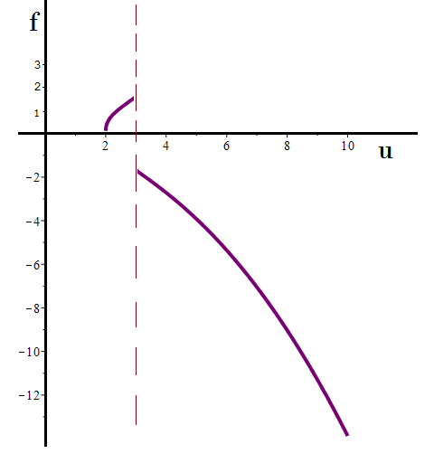
Figure 1: Two functions $f(u)\equiv f(\varphi(u))$ for $\mu=b_{0}=1$. Here the $\varphi(u)$ correspondence obeys in our notations: $\varphi(2)=-\varphi_{2}<0$, $\varphi(3)=0$, and $\varphi(+\infty)=\varphi_{1}>0$.

Let us consider the first case $c_{0}<0$. Due to

$$\varphi_{1}-\varphi(u)\sim{\rm const}\cdot u^{-1/3}$$ (4.38)

as $u\to+\infty$ (see (4.20), (4.31), and (4.32)), and (4.37), we obtain

$$f(\varphi)\sim-C_{f,1}\left(\varphi_{1}-\varphi\right)^{-7}$$ (4.39)

as $\varphi\to\varphi_{1}$. Here $C_{f,1}>0$ is constant.

Now we use the asymptotical relation

$$f(u)-f\left(3\mu+0\right)\sim\dot{f}\left(3\mu+0\right)\left(u-3\mu\right),$$ (4.40)

as $u\to 3\mu+0$. We denote

$${}f_{0}=-f\left(3\mu+0\right)=f\left(3\mu-0\right)$$

$${}\hskip 72.26999pt=|c_{0}|\frac{108}{7}\mu^{7/3}>0.$$ (4.41)

Due to $\varphi\sim{\rm const}\cdot\left(u-3\mu\right)^{3/2}$ as $u\to 3\mu$ (see (4.18), (4.31)), (4.40), and (4.41), we get

$$f(\varphi)+f_{0}\sim-C_{f,+}\varphi^{2/3},$$ (4.42)

as $\varphi\to+0$. Here $C_{f,+}>0$ is a constant proportional to ($\dot{f}\left(3\mu+0\right)<0$).

Let us consider the second case $c_{0}>0$. By using the asymptotical relations

$$f(u)-f\left(3\mu-0\right)\sim\dot{f}\left(3\mu-0\right)\left(u-3\mu\right),$$ (4.43)

as $u\to 3\mu$, and $(-\varphi)\sim{\rm const}\left(3\mu-u\right)^{3/2}$, as $u\to 3\mu$, (see (4.25), (4.31)) and (4.41), we are led to the following asymptotical relation:

$$f(\varphi)-f_{0}\sim-C_{f,-}\left(-\varphi\right)^{2/3},$$ (4.44)

as $\varphi\to-0$. Here $C_{f,-}>0$ is a constant, proportional to $\dot{f}\left(3\mu-0\right)>0$.

Now we rewrite the asymptotic relation (4.35). By using $\varphi+\varphi_{2}\sim{\rm const}\cdot(u-2\mu)^{1/6}$ (see (4.27) and (4.33)), we obtain

$$f(\varphi)\sim C_{f,2}\left(\varphi+\varphi_{2}\right)^{2},$$ (4.45)

as $\varphi\to-\varphi_{2}$. Here $C_{f,2}>0$ is constant.

For $c_{0}<0$ the coupling function $f(\varphi)$ is defined on the interval $(0,\varphi_{1})$. It is negative-definite, $f(\varphi)<0$, and unbounded since $f(\varphi)\to-\infty$ as $\varphi\to\varphi_{1}$. For $c_{0}>0$ the function $f(\varphi)$ is defined on the interval $(-\varphi_{2},0)$. It is posive-definite and bounded since $0<f(\varphi)<f_{0}$. At $\varphi\to-\varphi_{2}$ it vanishes: $f(\varphi)\to+0$.

4.4 The potential function

Now we consider the potential function. Here we keep our agreement (4.31). We start with the relation (4.13) for $U(u)$.

At $c_{0}<0$ and $u>3\mu$ we obtain

$$U(u)\sim-\left|c_{0}\right|\frac{16}{3}u^{-8/3}$$ (4.46)

as $u\to+\infty$, and

$$U(u)\sim-\left|c_{0}\right|\frac{16}{81}\mu^{-8/3}\left(u-3\mu\right),$$ (4.47)

as $u\to 3\mu$. For $c_{0}>0$ and $2\mu<u<3\mu$, we get

$$U(u)\sim-c_{0}\frac{16}{81}\mu^{-8/3}\left(3\mu-u\right),$$ (4.48)

as $u\to 3\mu$ and

$$U(u)\sim-c_{0}\frac{2}{3}\mu^{-1}\left(u-2\mu\right)^{-2/3},$$ (4.49)

as $u\to 2\mu$.

The functions $U(u)$ corresponing to $c_{0}>0$ and $c_{0}<0$ are depicted in Fig. 2 (for $\mu=1$ and $b_{0}=1$).

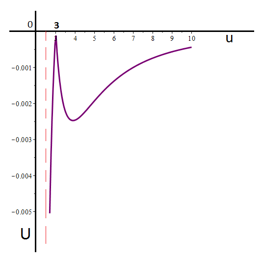
Figure 2: Two functions $U(u)\equiv U(\varphi(u))$ for $\mu=b_{0}=1$. The function $\varphi(u)$ obeys: $\varphi(2)=-\varphi_{2}$, $\varphi(3)=0$, and $\varphi(+\infty)=\varphi_{1}$.

In the case $c_{0}<0$ the point of minimum is reached at

$$u_{\ast}=\frac{3\sqrt{33}+45}{16}\approx 3.8896,$$ (4.50)

with $U\left(u_{\ast}\right)\equiv U_{\ast}=-(16/3)|c_{0}|N_{\ast}$, where
$N_{\ast}\approx 0.0098908$, obtained as

$${}N_{\ast}=N_{1}/N_{2},$$

$${}N_{1}=\Bigl{(}11072\sqrt{33}+49344\Bigr{)}\Bigl{(}\frac{3\sqrt{33}+45}{16}-2\Bigr{)}^{1/3},$$

$${}N_{2}=\frac{\left(3\sqrt{33}+45\right)\left(645165\sqrt{33}+3765123\right)}{16}$$

$${}\hskip 28.45274pt-1290330\sqrt{33}-7530246.$$ (4.51)

Now we consider the potential function in terms of the original variable, i.e., $U(\varphi)$. For $c_{0}<0$, we find

$$U(\varphi)\sim C_{U,1}(\varphi_{1}-\varphi)^{8},$$ (4.52)

as $\varphi\to\varphi_{1}$, where $C_{U,1}<0$ is constant, and

$$U(\varphi)\sim C_{U,0}\varphi^{2/3},$$ (4.53)

as $\varphi\to+0$, where $C_{U,0}<0$ is constant. For $c_{0}>0$ we obtain

$$U(\varphi)\sim C_{U,0}\left(-\varphi\right)^{2/3},$$ (4.54)

as $\varphi\to-0$, and

$$U(\varphi)\sim C_{U,2}(\varphi+\varphi_{2})^{-4},$$ (4.55)

as $\varphi\to-\varphi_{2}$, where $C_{U,2}<0$ is constant.

We see that in both cases $U(\varphi)<0$. For $c_{0}<0$ we obtain

$$U(\varphi)\geq U\left(\varphi_{\ast}\right)=U_{\ast},$$ (4.56)

where $\varphi_{\ast}=\varphi\left(u_{\ast}\right)\approx 0,01145$, i.e., the potential $U(\varphi)$ is bounded. For $c_{0}>0$ we get $U(\varphi)\to-\infty$ as $\varphi\to-\varphi_{2}$, i.e., potential is unbounded.

5 Conclusions

We have studied the 4D gravitational model with a real scalar field $\varphi$, Einstein and Gauss-Bonnet terms. The action contains the potential term $U(\varphi)$ and the Gauss-Bonnet coupling function $f(\varphi)$. For a special (static) spherically symmetric metric $ds^{2}=du^{2}/A(u)-A(u)dt^{2}+u^{2}d\Omega^{2}$, with a given redshift function $A(u)>0$ ($u>0$ is a radial coordinate), we have verified the so-called reconstruction procedure suggested by Nojiri and Nashed [15], according to which there exists a pair of $U(\varphi)$ and $f(\varphi)$, described by certain implicit relations, which leads us to exact solutions to the equations of motion with a given metric governed by $A(u)$. Here we have confirmed that all relations in Ref. [15] for $f(\varphi(u))$ and $\varphi(u)$ are correct, but the expression for $U(\varphi(u))$ contains a typo which is eliminated in this paper.

We have applied the reconstruction procedure to the external Schwarzschild black hole metric with the gravitational radius $2\mu>0$ and $u>2\mu$. Using the “no-ghost” restriction (i.e., reality of $\varphi(u)$), we have found two sets of $(U(\varphi),f(\varphi))$. The first one gives us the Schwarzschild metric defined at $u>3\mu$, and the second one describes the Schwarzschild metric defined for $2\mu<u<3\mu$. In both cases the potential $U(\varphi)$ is negative. For the first set $(U(\varphi),f(\varphi))$ with $\varphi\in(0,\varphi_{1})$, the potential $U(\varphi)$ is bounded, and the coupling function $f(\varphi)<0$ is unbounded, while for the second set $(U(\varphi),f(\varphi))$ with $\varphi\in(-\varphi_{2},0)$ the potential $U(\varphi)$ is unbounded, and the coupling function $f(\varphi)>0$ is bounded.

It should be noted that here $3\mu$ is the radius of the photon sphere, which means that the two domains, where we have real scalar field solutions, are separated by the photon sphere. The general analysis of Ref. [15] and its application to the Hayword black hole solution indicates the possibility to solve the ghost avoidance problem at least locally, i.e,. in two ranges of the radial variable: $(r_{h},r_{1,*})$ and $(r_{2,*},+\infty)$, where $r_{h}$ is the horizon radius, and $r_{h}<r_{1,*}<r_{2,*}$. The problem of enlarging these intervals such that $r_{1,*}=r_{2,*}=r_{*}$ was not studied in Ref. [15]. This problem may be addressed in the forthcoming publications devoted to the reconstruction procedure for a general class of static spherically symmetric metrics $ds^{2}=du^{2}/A(u)-A(u)dt^{2}+C(u)d\Omega^{2}$ (with the areal function $C(u)>0$), with application to dilatonic black holes, e.g., those from [16, 17].

We note also that the reconstruction problem for general sperically symmetric metrics which appear in sEGB model was explored (up to resolving of the ghost avoiding problem) in Ref. [18]. Meanwhile, it was shown in Ref. [19] that arbitrary static spherically symmetric metric may be presented (though, in local parts) as a solution to equations of motion of some scalar tensor theory belonging to the class of Bergmann et al. In Ref. [20] and in some other papers the authors were able to present an arbitrary static spherically symmetric metric obeying $R^{0}_{0}=R^{1}_{1}$ as coming from a “magnetic” solution of certain $GR+NED$ theory ($NED$ means nonlinear electrodynamics).

Funding

The research was funded by RUDN University, scientific project number FSSF-2023-0003.

Conflict of interest

The authors declare that they have no conflicts of interest.

References

- [1] B. Zwiebach, Phys. Lett. B 156, 315 (1985).
- [2] E.S. Fradkin and A.A. Tseytlin, Phys. Lett. B 158, 316-322 (1985).
- [3] E.S. Fradkin and A.A. Tseytlin, Phys. Lett. B 160, 69-76 (1985).
- [4] D. Gross and E. Witten, Nucl. Phys. B 277, 1 (1986).
- [5] P. Kanti, N.E. Mavromatos, J. Rizos, K. Tamvakis and E. Winstanley, Phys. Rev. D 54 , 5049 (1996).
- [6] P. Kanti, N. E. Mavromatos, J. Rizos, K. Tamvakis and E. Winstanley, Phys. Rev. D 57, 6255 (1998).
- [7] R. Konoplya, T. Pappas, and A. Zhidenko, Phys. Rev. D 101, 044054 (2020).
- [8] B. Kleihaus and J. Kunz, Astronomy Reports 67: S108-S114 (2024).
- [9] K.A. Bronnikov and E. Elizalde, Phys. Rev. D 81, 044032 (2010).
- [10] B.P. Abott et al., Phys. Rev. Lett. 116 (6), 061102 (2016).
- [11] V. Perlick and O. Yu. Tsupko, Physics Reports, 947, 1-39 (2022).
- [12] R. Konoplya and A. Zhidenko, Rev. Mod. Phys. 83 (3), 793 (2011).
- [13] P.V.P. Cunha, C.A.R. Herdeiro, E. Radu, and H.F. Runarsson, Phys. Rev. Lett. 125 (21), 211102 (2015).
- [14] R.A. Konoplya, A.F. Zinhailo, and Z. Stuchlik, Phys. Rev. D 99, 124042 (2019).
- [15] S. Nojiri and G.G.L. Nashed, Phys. Rev. D 108 (2), 024014 (2023); arXiv: 2306.14162 [gr-qc].
- [16] A.N. Malybayev, K.A. Boshkayev, and V.D. Ivashchuk, Eur. Phys. J. C 81, Id. 475, 1-12 (2021).
- [17] V.D. Ivashchuk, A.N. Malybayev, G.S. Nurbakova, and G. Takey, Grav. Cosmol. 29, No. 4, 411-418 (2023).
- [18] G.G.L. Nashed and S. Nojiri, Eur. Phys. J. C 83, No.1, Id. 68, 1-16 (2023).
- [19] K.A. Bronnikov, K. Badalov, and R. Ibadov, Grav. Cosmol. 29, No. 1, 43–49 (2023); arXiv: 2212.04544.
- [20] K.A. Bronnikov, Regular black holes sourced by nonlinear electrodynamics, in: “Regular Black Holes. Towards a New Paradigm of Gravitational Collapse,” (Ed. by Cosimo Bambi, Springer Series in Astrophysics and Cosmology (SSAC)) p. 37–67; arXiv: 2211.00743.