Enhancing Dynamic CT Image Reconstruction with Neural Fields Through Explicit Motion Regularizers

Abstract

Image reconstruction for dynamic inverse problems with highly undersampled data poses a major challenge: not accounting for the dynamics of the process leads to a non-realistic motion with no time regularity. Variational approaches that penalize time derivatives or introduce PDE-based motion model regularizers have been proposed to relate subsequent frames and improve image quality using grid-based discretization. Neural fields are an alternative to parametrize the desired spatiotemporal quantity with a deep neural network, a lightweight, continuous, and biased towards smoothness representation. The inductive bias has been exploited to enforce time regularity for dynamic inverse problems resulting in neural fields optimized by minimizing a data-fidelity term only. In this paper we investigate and show the benefits of introducing explicit PDE-based motion regularizers, namely, the optical flow equation, in 2D+time computed tomography for the optimization of neural fields. We also compare neural fields against a grid-based solver and show that the former outperforms the latter.

Keywords Dynamic Inverse Problems  $\cdot$ Neural fields  $\cdot$ Explicit regularizer  $\cdot$ Optical flow

1 Introduction

In many imaging tasks, the target object changes during the data acquisition. In clinical settings for instance, imaging techniques such as Computed Tomography (CT), Positron Emission Tomography (PET) or Magnetic Resonance Imaging (MRI) are used to study moving organs such as the heart or the lungs. Usually, the acquired data is a time series collected at several discretized times $0=t_{0}<t_{1}<\ldots<t_{N_{T}}=T$ but the rapid and constant motion of these organs prevents the scanners from taking enough measurements in a single time instant $t_{i}$ and thus, measurements are highly undersampled in space. One way to proceed is by neglecting the time component and solving several static inverse problems. However, the lack of information makes this naive frame-by-frame reconstruction a severely ill-posed problem leading to a poor reconstruction. It is therefore necessary to seek a spatiotemporal quantity with coherence between subsequent frames whose reconstruction takes into account the dynamic of the process. Typical approaches are variational methods that penalize first-order temporal derivative of the sequence [1, 2, 3] and variational methods that incorporate explicit motion models based on partial differential equations (PDEs) [4, 5, 6, 7]. We focus on the latter focus, which aims at penalizing unrealistic dynamics at the cost of introducing the motion as an additional quantity to discover. We refer to [8] for an extensive review of dynamic inverse problems. The aforementioned papers use classical grid-based representations of the spatiotemporal image which suffer from two issues: (1) their lack of regularity which motivates the use of regularizers such as Tikhonov, total variation, or the previously mentioned motion model, and (2) their complexity grows exponentially with the dimension and polynomially with the discretization due to the curse of dimensionality which can incur in memory burden.

In the last couple of years, coordinate-based multilayer perceptrons (MLPs) have been employed as a new way of parameterizing quantities of interest. In computer vision, these are referred to as neural fields or implicit neural representations [9, 10], while the term Physics-Informed Neural Networks (PINNs) has been adopted when solving PDEs [11, 12]. The main idea is to use a neural network $u_{\theta}$ with trainable weights $\theta$ as an ansatz for the solution of the problem. It takes as input a low-dimensional point in the domain $x\in\Omega$, e.g., a pixel location, and outputs the value $u_{\theta}(x)$ at that point. The problem is then rephrased as a non-convex optimization that seeks optimal weights $\theta$. The method requires training a neural network for every new instance, thus, it is said to be self-supervised and differs from the usual learning framework where a solution map is found by training a network over large datasets. Applications of neural fields include image reconstruction in CT [13, 14, 15], MRI [16, 17, 18, 19, 20], image registration [21, 22, 23], continuous shape representation via signed distance functions [24] and volume rendering [25] among others.

It is well-known that, under mild conditions, neural networks can approximate functions at any desired tolerance [26], but their widespread use has been justified by other properties such as (1) the implicit regularization they introduce, (2) overcoming the curse of dimensionality, and (3) their lightweight, continuous and differentiable representation. In [27, 28] it is shown that the amount of weights needed to approximate the solution of particular PDEs grows polynomially on the dimension of the domain. For the same reason, only a few weights can represent complex images, leading to a compact and memory-efficient representation. Finally, numerical experiments and theoretical results show that neural fields tend to learn smooth functions early during training [29, 30, 31]. This is both advantageous and disadvantageous: neural fields can capture smooth regions of natural images but will struggle at capturing edges. The latter can be overcome with Fourier feature encoding [32].

In the context of dynamic inverse problems and neural fields, most of the literature relies entirely on the smoothness introduced by the network on the spatial and temporal variables to get a regularized solution. This allows minimizing a data-fidelity term only without considering any explicit regularizers. Applications can be found on dynamic cardiac MRI in [17, 20, 19], where the network outputs the real and imaginary parts of the signal, while in [18] the neural field is used to directly fit the measurements and then inference is performed by inpainting the k-space with the neural field and taking the inverse Fourier transform. In [33, 34] neural fields are used to solve a photoacoustic tomography dynamic reconstruction emphasizing their memory efficiency. In [15], a 3D+time CT inverse problem is addressed with a neural field parametrizing the initial frame and a polynomial tensor warping it to get the subsequent frames. To the best of our knowledge, it is the only work making use of neural fields and a motion model via a deformable template.

In this paper, we investigate the performance of neural fields regularized by explicit PDE-based motion models in the context of dynamic inverse problems in CT in a highly undersampled measurement regime with two dimensions in space. Motivated by [4] and leveraging automatic differentiation to compute spatial and time derivatives, we study the optical flow equation as an explicit motion regularizer imposed as a soft constraint as in PINNs. Our findings are based on numerical experiments and are summarized as follows:

• An explicit motion model constraints the neural field into a physically feasible manifold improving the reconstruction when compared to a motionless model.

• Neural fields outperform grid-based representations in the context of dynamic inverse problems in terms of the quality of the reconstruction.

• We show that, once the neural field has been trained, it generalizes well into higher resolutions.

The paper is organized as follows: in section 2 we introduce dynamic inverse problems, motion models and the optical flow equation, and the joint image reconstruction and motion estimation variational problem as in [4]; in section 3 we state the main variational problem to be minimized and study how to minimize it with neural fields and with a grid-based representation; in section 4 we study our method on a synthetic phantom which, by construction, perfectly satisfies the optical flow constraint, and show the improvements given by explicit motion regularizers; we finish with the conclusions in section 5.

2 Dynamic Inverse Problems in Imaging

The development of imaging devices has allowed us to obtain accurate images with non-invasive methods, which has been particularly exploited in areas such as biomedical imaging with Computed Tomography, Magnetic Resonance Imaging, Positron Emission Tomography, etc. Those methods collect measurements from where the imaged object can be recovered. In (static) inverse problems, we aim to reconstruct a quantity $u:\Omega\subset\mathbb{R}^{d}\to\mathbb{R}$ from measurements $f$ by solving an equation of the form

$$Ku+\varepsilon=f,$$ (1)

where $K$ is the forward operator modelling the imaging process and $\varepsilon$ is some noise. For dynamic inverse problems, the time variable is included and thus we seek a time-dependent quantity $u:\Omega\times[0,T]\to\mathbb{R}$ solving an equation of the form

$$K(t)[u(\cdot,t)](\cdot)+\varepsilon=f(\cdot,t),\quad\text{in }\Omega^{\prime}\times[0,T],$$ (2)

where $K$ now is a potentially time-dependent forward operator modelling the imaging process (e.g., a rotating CT scanner).

When the motion is slow compared to the acquisition speed, it is possible to take enough measurements to get a reconstruction by neglecting the time variable, considering the static inverse problem (1) instead, and solving for each $t$ a variational problem of the form

$$\min_{u(\cdot,t)}\mathcal{D}(u(\cdot,t),f(\cdot,t))+\alpha\mathcal{R}(u(\cdot,t)),\quad t\in[0,T],$$

where $\mathcal{D}$ represents a data-fidelity term measuring how well equation (1) for a particular time instance $t$ is satisfied and whose choice depends on the nature of the noise, e.g., $L^{2}$ error for gaussian noise or Kullback-Leibler divergence for Poisson noise. $\mathcal{R}$ is a regularization term such as the total variation [35] that adds prior information on $u(\cdot,t)$, and $\alpha>0$ is a regularization parameter balancing both terms.

However, when the imaged object undergoes some dynamics during measurement acquisition, then the scanner may fail at sampling enough measurements at a certain time $t$ and using the previous time-independent variational formulation will lead to a poor reconstruction with artifacts even with the use of regularizers due to the lack of enough measurements. This has motivated adding temporal regularity in the solution by introducing motion models [4, 6]. Such models aim to solve a joint variational problem with the unknowns being the image sequence $u:\Omega\times[0,T]\to\mathbb{R}$ and the motion given, for instance, by the velocity field $v:\Omega\times[0,T]\to\mathbb{R}^{d}$.

2.1 Motion Model

A motion model describes the relation between pixel intensities of the sequence and the velocity flow from frame to frame through an equation of the form $r(u,v)=0$ in $\Omega\times[0,T]$. Its choice is application-dependent, for instance, the continuity equation is a common choice for 3D problems in space while the optical flow equation is more suitable for 2D problems. These models are typically employed for the task of motion estimation, this is, given the image sequence $u$, to get the velocity flow. For example the optical flow equation reads as

$$r(u,v):=\partial_{t}u+v\cdot\nabla v=0,\quad\text{ in }\Omega\times[0,T].$$

It is derived from the brightness constancy assumption, this is, pixels keep constant intensity along their trajectory in time. This model poses only one equation for $d$ unknowns, the components of the velocity field, leading to an underdetermined set of equations. This is solved by considering a variational problem in $v$ with a regularization term:

$$\min_{v}\mathcal{A}(r(u,v))+\beta\mathcal{S}(v),$$ (3)

where $\mathcal{A}$ is a metric measuring how well the equation $r(u,v)=0$ is satisfied, $\mathcal{S}$ is a regularizer, and $\beta>0$ is the regularization parameter balancing both terms. This variational model was firstly introduced in [36] with $\mathcal{A}$ the $L^{2}$ norm and the regularizer as the $L^{2}$ norm of the gradient. Since then, different even non-smooth norms and regularizers have been tried, for instance, in [37] the $L^{1}$ norm is used to impose the motion model, and in [38] it is employed the $L^{1}$ norm and the total variation for regularization.

2.2 Joint Image Reconstruction and Motion Estimation

To solve highly-undersampled dynamic inverse problems, in [4] it is proposed a joint variational problem where not only the dynamic process $u$ is sought, but also the underlying motion expressed in terms of a velocity field $v$. The main hypothesis is that a joint reconstruction can enhance the discovery of both quantities, image sequence and motion, improving the final reconstruction compared to motionless models. Hence, the sought solution $(u^{*},v^{*})$ is a minimizer for the variational problem given below:

$$\min_{u,v}\mathcal{D}(u,f)+\alpha\mathcal{R}(u)+\beta\mathcal{S}(v)+\gamma\mathcal{A}(r(u,v)),$$ (4)

with $\alpha,\beta,\gamma>0$ being regularization parameters balancing the four terms. In [4], the domain is 2D+time, and among others, it is shown how the purely motion estimation task of a noisy sequence can be enhanced by solving the joint task of image denoising and motion estimation.

This model was further employed for 2D+time problems in [6] and [7]. In the former it is studied its application on dynamic CT with sparse limited-angles and it is studied both $L^{1}$ and $L^{2}$ norms for the data fidelity term, with better results for the former. In the latter, the same logic is used for dynamic cardiac MRI. In 3D+time domains, we mention [39] and [40] for dynamic CT and dynamic photoacoustic tomography respectively.

3 Methods

Depending on the nature of the noise, different data-fidelity terms can be considered. In this work, we consider Gaussian noise $\varepsilon$, so, to satisfy equation (2) we use an $L^{2}$ distance between predicted measurements and data

$$\mathcal{D}(u,f):=\displaystyle\int_{0}^{T}\dfrac{1}{2}\|K(t)[u(\cdot,t)](\cdot)-f(\cdot,t)\|^{2}_{L^{2}(\Omega^{\prime})}dt.$$

Since $u$ represents a natural image, a suitable choice for regularizer $\mathcal{R}$ is the total variation to promote noiseless images and capture edges:

$$\mathcal{R}(u):=\displaystyle\int_{0}^{T}\text{TV}(u(\cdot,t))dt.$$

For the motion model, we consider the optical flow equation (5), and to measure its distance to 0 we use the $L^{1}$ norm. For the regularizer in $v$ we consider the total variation on each of its components.

$$\mathcal{A}(r(u,v)):=\|r(u,v)\|_{L^{1}(\Omega\times[0,T])},\quad\mathcal{S}(v):=\displaystyle\sum_{p=1}^{d}\displaystyle\int_{0}^{T}\text{TV}(v^{p}(\cdot,t))dt.$$ (5)

Thus, the whole variational problem reads as follows:

$$\min_{u,v}\int_{0}^{T} \dfrac{1}{2}\|K(t)[u(\cdot,t)](\cdot)-f(\cdot,t)\|^{2}_{L^{2}(\Omega^{\prime})}+\alpha\text{TV}(u(\cdot,t))+$$ (6)

$$\beta\sum_{p=1}^{d}\text{TV}(v^{p}(\cdot,t))+\gamma\|\partial_{t}u(\cdot,t)+v(\cdot,t)\cdot\nabla u(\cdot,t)\|_{L^{1}(\Omega)}dt.$$

We now describe how to solve this variational problem numerically for the neural field and the grid-based representation. In both cases, we proceed with a discretize-then-optimize approach and assume that measurements $f\in\mathbb{R}^{N_{T}\times N^{\prime}}$ are given on a uniform grid.

3.1 Numerical evaluation with Neural Fields

Since Tomosipo acts on voxelated images and the measurements are given on a grid as well, the predicted measurement at frame $i$ requires the evaluation of the network at points on a cartesian grid to get a grid-based representation $(u_{\theta})_{i}:=\{u_{\theta}(x_{j},t_{i})\}_{j=1,\ldots,N}$. The operator $K(t_{i})$ maps $(u_{\theta})_{i}\in\mathbb{R}^{N}$ to $K(t_{i})(u_{\theta})_{i}\in R^{N^{\prime}}$, for $i=1,\ldots,N_{T}$. To simplify the notation, we let $(Ku_{\theta})_{i}:=K(t_{i})(u_{\theta})_{i}$. For the regularization terms, since neural fields are mesh-free, they can be evaluated at any point of the domain. Additionally, derivatives can be computed with no error through automatic differentiation, thus, these are exact and there is no need to use finite difference schemes. We then discretize (6) as follows:

$$\min_{\theta,\phi} \dfrac{T}{N_{T}}\dfrac{|\Omega^{\prime}|}{N^{\prime}}\sum_{i=1}^{N_{T}}\sum_{j=1}^{N^{\prime}}\dfrac{1}{2}((Ku_{\theta})_{ij}-f_{ij})^{2}+$$ (7)

$$\mathbb{E}_{(x,t)\sim U(\Omega\times[0,T])}\left[\alpha\|\nabla u_{\theta}(x,t)\|_{2}+\beta\left(\displaystyle\sum_{p=1}^{d}\|\nabla v_{\phi}^{p}(x,t)\|_{2}\right)+\gamma|\partial_{t}u_{\theta}(x,t)+v_{\phi}(x,t)\cdot\nabla u_{\theta}(x,t)|\right].$$

The evaluation of the data fidelity term in (7) would require first the evaluation of the network at $N_{T}\times N$ fixed grid-points to get the image $\{(u_{\theta})_{ij}\}_{i=1,\ldots,N_{T};j=1,\ldots,N}$, and, second, the application of the forward model $K(t_{i})$ to each frame $\{(u_{\theta})_{i}\}_{i=1,\ldots,N_{T}}$. This might be expensive and time-consuming, so, we proceed with a stochastic-gradient-descent-like approach in time instead, this is, at each iteration, the network is evaluated at a randomly sampled frame, say, the $i$-th frame, with points of the form $\{(x_{j},t_{i})\}_{j=1,\ldots,N}$ to get the representation of the image at time $t_{i}$. Then, the forward model is applied on this frame only and the parameters are updated to minimize the difference between predicted data and the measured data $f_{i}$ at this frame. One epoch then consists of $N_{T}$ iterations. This represents considerable benefits in terms of memory since the whole scene is never explicitly represented in the whole space-time grid but adds variability during training. Additionally, at each iteration, we sample $N_{c}$ collocation points of the form $\{(x^{c}_{l},t^{c}_{l})\}_{l=1\ldots,N_{c}}$, using a Latin Hypercube Sampling strategy [41] on the domain $\Omega\times[t_{i}-\delta,t_{i}+\delta]$, for some $\delta>0$, with $t_{i}$ the frame used to evaluate the data fidelity term as explained previously. In conclusion, at the $k$-th iteration, some $i$-th frame is sampled and the parameters of the network are updated by taking the gradient with respect to $\theta$ and $\phi$ of the following function:

$$\begin{array}[]{l}\dfrac{T}{N_{T}}\dfrac{|\Omega^{\prime}|}{N^{\prime}}\displaystyle\sum_{j=1}^{N^{\prime}}\dfrac{1}{2}((Ku_{\theta})_{ij}-f_{ij})^{2}+\\ \dfrac{T|\Omega|}{N_{c}}\displaystyle\sum_{l=1}^{N_{c}}\left[\alpha\|\nabla u_{\theta}(x^{c}_{l},t^{c}_{l})\|_{2}+\beta\left(\displaystyle\sum_{p=1}^{d}\|\nabla v_{\phi}^{p}(x^{c}_{l},t^{c}_{l})\|_{2}\right)+\gamma|\partial_{t}u_{\theta}(x^{c}_{l},t^{c}_{l})+v_{\phi}(x^{c}_{l},t^{c}_{l})\cdot\nabla u_{\theta}(x^{c}_{l},t^{c}_{l})|\right].\end{array}$$

Finally, we recall that the choice of $N_{c}$, the amount of collocation points sampled on each iteration, is not clear. One would like to sample as many points as possible to have a better approximation of the regularizer, however, this might be time-consuming and prohibitive in terms of memory because of the use of auto differentiation. Thus, we define the Sampling Rate $SR$ as the rate between $N_{c}$ and the amount of points $N$ on the spatial grid:

$$SR:=\dfrac{N_{c}}{N}.$$ (8)

In the experiments, we use a sampling rate of 0.1.

3.2 Numerical evaluation with grid-based representation

In this section we briefly describe the numerical realization as in [4]. A uniform grid $\{(x_{j},t_{i})\}_{i=1,\ldots,N_{T};j=1,\ldots,N}\subset\Omega\times[0,T]$ is assumed. Next, the quantities of interest are vectorized as $u\in\mathbb{R}^{N_{T}\times N}$, $v\in\mathbb{R}^{N_{T}\times N\times d}$, such that, $u_{ij}$ denotes the value of $u$ at the point $(x_{j},t_{i})$. The operator $K(t_{i})$ maps $u_{i}\in\mathbb{R}^{N}$ to $K(t_{i})u_{i}\in R^{N^{\prime}}$, for $i=1,\ldots,N_{T}$. To simplify the notation, we let $(Ku)_{i}:=K(t_{i})u_{i}$. Finite difference schemes are employed to compute the corresponding derivatives, namely, $D$ and $D_{t}$ denote the discrete gradients in space and time respectively (these could be forward or centred differences). Thus $(Du)\in\mathbb{R}^{N_{T}\times Nd}$, $(D_{t}u)\in\mathbb{R}^{N_{T}\times N}$, and $(Dv^{p})\in\mathbb{R}^{N_{T}\times N\times d}$. Using the previous, the variational problem is discretized as

$$\min_{u,v} \dfrac{T}{N_{T}}\dfrac{|\Omega^{\prime}|}{N^{\prime}}\sum_{i=1}^{N_{T}}\sum_{j=1}^{N^{\prime}}\dfrac{1}{2}((Ku)_{ij}-f_{ij})^{2}+$$

$$\dfrac{T}{N_{T}}\dfrac{|\Omega|}{N}\sum_{i=1}^{N_{T}}\sum_{j=1}^{N}\left[\alpha\|(Du)_{ij}\|_{2}+\beta\left(\displaystyle\sum_{p=1}^{d}\|(Dv^{p})_{ij}\|_{2}\right)+\gamma|(D_{t}u)_{ij}+v_{ij}\cdot(Du)_{ij}|\right].$$

It can be easily seen that this problem is biconvex, hence, in [4], the proposed optimization routine updates the current iteration $(u^{k},v^{k})$ by alternating between the following two subproblems:

• Problem in $u$. Fix $v^{k}$ and solve the following minimization problem for $u$:

  $$u^{k+1}:=\operatorname*{arg\,min}_{u} \dfrac{T}{N_{T}}\dfrac{|\Omega^{\prime}|}{N^{\prime}}\sum_{j=1}^{N^{\prime}}\dfrac{1}{2}((Ku)_{ij}-f_{ij})^{2}+\dfrac{T}{N_{T}}\dfrac{|\Omega|}{N}\sum_{i=1}^{N_{T}}\sum_{j=1}^{N}\alpha\|(Du)_{ij}\|_{2}+\gamma|(D_{t}u)_{ij}+v^{k}_{ij}\cdot(Du)_{ij}|.$$ (9)

• Problem in $v$. Fix $u^{k+1}$ and solve the following minimization problem for $v$:

  $$v^{k+1}:=\operatorname*{arg\,min}_{v}\dfrac{T}{N_{T}}\dfrac{|\Omega|}{N}\displaystyle\sum_{i=1}^{N_{T}}\displaystyle\sum_{j=1}^{N}\beta\left(\displaystyle\sum_{p=1}^{d}\|(Dv^{p})_{ij}\|_{2}\right)+\gamma|(D_{t}u^{k+1})_{ij}+v_{ij}\cdot(Du^{k+1})_{ij}|.$$ (10)

Each subproblem is convex with non-smooth terms involved that can be solved using the Primal-Dual Hybrid Gradient (PDHG) algorithm [42]. We refer to [4] for the details.

4 Numerical Experiments

In our numerical experiments, we make use of Tomosipo [43] to compute the X-ray transform and its transpose for both, the neural field and the grid-based representation. This library provides an integration of the ASTRA-toolbox [44, 45] with PyTorch for deep learning purposes. We make use of fan-beam projection geometry for the forward operator. The architecture for the neural networks in $u$ and $v$ consists of an input layer of size 3, then Fourier feature mappings of the form $(x,t)\to(\Gamma_{1}(x),\Gamma_{2}(t))\in\mathbb{R}^{128}$, then three hidden layers of size 128 and we finish with an output layer of size 1 for $u$ and size $2$ for $v$. Here $\Gamma_{1}(x):=(\sin(2\pi B_{x}x),\cos(2\pi B_{x}x))$ and $\Gamma_{2}(T):=(\sin(2\pi B_{t}t),\cos(2\pi B_{t}t))$, with the matrices $B_{x}$ and $B_{t}$ having non-trainable entries $(B_{x})_{ij}\sim\mathcal{N}(0,\sigma_{x}^{2})$ and $(B_{t})_{ij}\sim\mathcal{N}(0,\sigma_{t}^{2})$. We found $\sigma_{x}=\sigma_{t}=0.1$ to give the best results. The neural networks are trained with Adam optimizer with initial learning rate $10^{-3}$.

4.1 Synthetic experiments

Here we assess our method and compare it against the grid-based one with two synthetic experiments. The considered domain is the square $\Omega=[-1,1]^{2}$. To define the ground-truth phantom $u$ we proceed as follows:

• Let $u_{0}:\Omega\to[0,1]$ be the initial frame, i.e., we let $u(x,0):=u_{0}(x)$.

• Define $\varphi:\Omega\times[0,T]\to\Omega$ describing the motion of the process. It takes a point $(x_{0},t)\in\Omega\times[0,T]$ and outputs $\varphi(x_{0},t)=x\in\Omega$, the new position of $x_{0}$ at time $t$. For each time we can define the function $\varphi_{t}:\Omega\to\Omega$ by $\varphi_{t}(x_{0})=\varphi(x_{0},t)$. We ask for $\varphi_{t}$ to be a diffeomorphism for every $t\in[0,T]$. Hence we can define the trajectory of the point $x_{0}$ as $t\to x(t)=\varphi_{t}(x_{0})$

• Define $u(x,t):=u_{0}(\varphi_{t}^{-1}(x))$.

The phantom thus generated solves exactly the optical flow equation with velocity field $v=\frac{d}{dt}\varphi$.

4.1.1 Two-squares phantom

The first phantom is depicted in figure 1 with two squares moving within an ellipsis-shaped background. The inverse of the motion for the squares on the left and right are $\varphi_{1}^{-1}$ and $\varphi_{2}^{-1}$ respectively, each one given by the following expressions:

$$\varphi_{1}^{-1}(x,y,t)=\begin{pmatrix}x-\frac{t}{5}\cos(2\pi t)\\ y-\frac{3t}{4}\sin(2\pi t)\end{pmatrix},\quad\varphi_{2}^{-1}(x,y,t)=\begin{pmatrix}x-0.3t\\ y-0.8t\end{pmatrix}.$$

From this, the velocity fields are easily expressed as:

$$v_{1}(x,y,t)=\begin{pmatrix}\frac{1}{5}\cos(2\pi t)-\frac{2\pi t}{5}\sin(2\pi t)\\ \frac{3}{4}\sin(2\pi t)+\frac{3\pi t}{2}\cos(2\pi t)\end{pmatrix},\quad v_{2}(x,y,t)=\begin{pmatrix}0.3\\ 0.8\end{pmatrix}.$$

$v_{1}$ produces a spiral-like motion for the square on the left and $v_{2}$ a constant diagonal motion for the square on the right. These are depicted in the second row of figure 1 (see remark 1 to understand this representation).

Remark 1

The second row in figure 1 represents the velocity field as follows: the coloured boundary frame indicates the direction of the velocity field. The intensities of the image indicate the magnitude of the vector. As an example, the square on the right moves constantly up and slightly to the right during the motion.

Measurements are obtained by sampling one random angle per frame and further corrupted with Gaussian noise with standard deviation $\sigma=0.01$. See the third row in figure 1. To highlight the necessity of motion models, two naive reconstructions are shown in the fourth row of figure 1. The one on the left corresponds to a time-static reconstruction, i.e., assuming that the squares are not moving. The result is an image that blurs those regions where the squares moved. The one on the right is a frame-by-frame reconstruction which, as expected, cannot get a reliable reconstruction from one projection only.

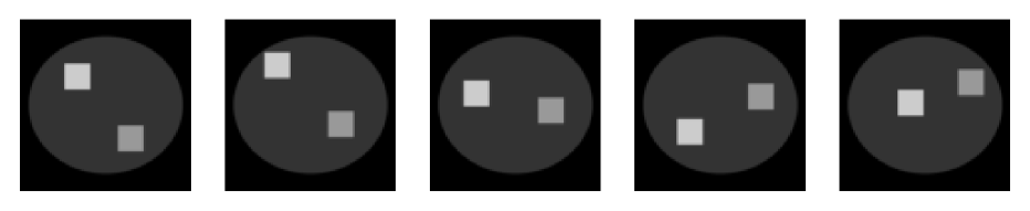
(a)

(b)

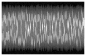
(c)

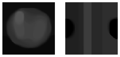
(d)

Figure 1: First row: ground truth image at frames 15, 35, 55, 75, 95 (out of 100). Second row: velocity field at frames 15, 35, 55, 75, 95 (out of 100). Third row: fan-beam measurements with one random angle projection per time instant. Fourth row left: reconstruction neglecting the time component. Fourth row right: frame-by-frame reconstruction from angle at $t=0$.

Effect of the motion regularization parameter $\gamma$.

We begin our study by choosing $\alpha,\beta=0$ and varying $\gamma\in\{0,10^{-5},10^{-4},10^{-3},10^{-2}\}$. In this case, we find that the best reconstruction in terms of PSNR is given by $\gamma=10^{-3}$. We show this reconstruction and the one with $\gamma=0$ in figure 2. The reconstruction with $\gamma=10^{-3}$ achieves a PSNR of 25.7 versus a PSNR of 22.08 for the implicitly regularized neural field. We also show in figure 3(a) how the PSNR changes during the optimization. The curves $\gamma=0$ and $\gamma=10^{-5}$ are the ones performing the worst since almost no motion model is being imposed. As we increase $\gamma$ the reconstruction improves and is consistently better than the motionless one. We mention however the variability of the metric during training which poses challenges as for when to stop training. We claim that this behaviour is due to the randomness coming from the collocation points and an increase in the sampling rate can alleviate it.

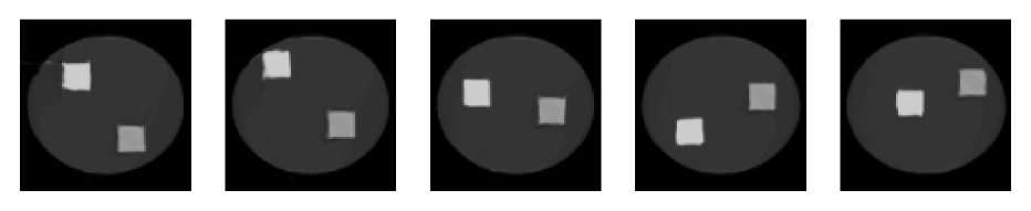
(a)

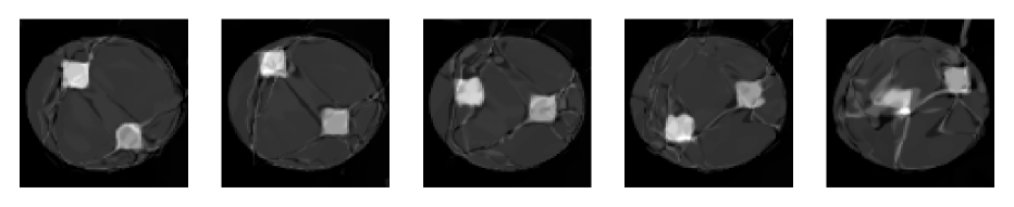
(b)

Figure 2: Reconstructions with neural fields. First row: prediction with neural field $(\alpha,\beta,\gamma)=(0,0,10^{-3})$, PSNR: 25.7. Second row: prediction with implicitly regularized neural field $(\alpha,\beta,\gamma)=(0,0,0)$, PSNR: 22.08.

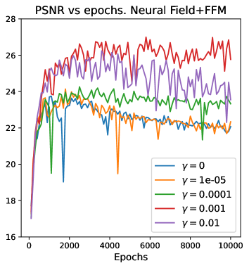
(a)

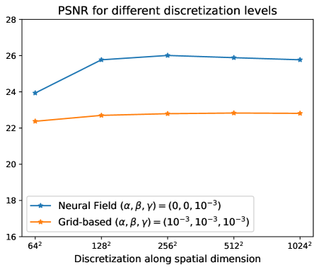
(b)

Figure 3: Left: Evolution of PSNR during training for different values of $\gamma$ and every 100 epochs (in our setting each epoch consists of 100 iterations). Right: PSNR along different discretization levels for neural field and grid-based representations.

Neural fields versus Grid-based method.

We now compare explicitly regularized neural fields against the grid-based method outlined in section 3.2. We do not consider the case $\alpha=\beta=0$ for the grid-based approach, since the lack of a TV regularizer leads to poor performance. For this approach, it was found that the choice $(\alpha,\beta,\gamma)=(10^{-3},10^{-3},10^{-3})$ led to the best results in terms of PSNR, achieving a value of 22.8. We try the same choice for the neural field representation in which case the PSNR is 24.1. Results are shown in figure 4. There it is clear that neural fields outperform the grid-based solution even for the choice of regularization parameters that led to the best behaviour for the grid-based method. Moreover, when comparing the choices $(\alpha,\beta,\gamma)=(10^{-3},10^{-3},10^{-3})$ and $(\alpha,\beta,\gamma)=(0,0,10^{-3})$ from the previous point it can be seen that adding the total variation regularizers on $u$ and $v$ has a negative effect in terms of PSNR for the image reconstruction task.

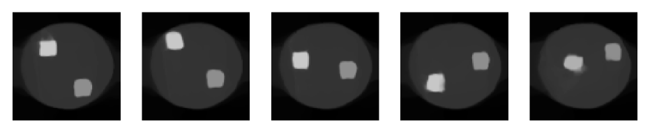
(a)

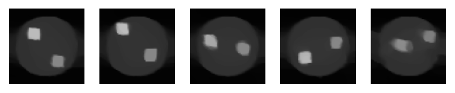
(b)

Figure 4: Reconstructions with different methods for the choice $(\alpha,\beta,\gamma)=(10^{-3},10^{-3},10^{-3})$. From left to right: frames 15, 35, 55, 75, 95 (out of 100). First row: prediction with neural field, PSNR: 24.1. Second row: prediction with grid-based representation, PSNR: 22.8.

Generalization into higher resolution.

We finish this section by assessing the continuous representation of the neural field and their generalization by comparing it against the ground truth at different resolutions. We recall that the neural field and the grid-based were optimized on a fixed grid of size $64\times 64$. Once trained the neural field can be evaluated at any resolution while the grid-based solution is interpolated into higher resolutions via the nearest neighbourhood method. The ground truth image originally defined at $1024\times 1024$ is downsampled to the corresponding resolutions for comparison. For the neural field we take the model with $(\alpha,\beta,\gamma)=(0,0,10^{-3})$ while for the grid-based method, we take the model with $(\alpha,\beta,\gamma)=(10^{-3},10^{-3},10^{-3})$. Results are shown in figure 3(b) where it can be seen that a larger increase in the quality of the reconstruction with respect to the resolution is given by the neural field solution.

5 Conclusion

In this work we studied neural fields for dynamic inverse problems. We saw how to enhance neural fields reconstruction for dynamic inverse problems by making use of explicit PDE-based motion regularizers, namely, the optical flow equation. Constraining the neural field to this physically feasible motion meant a significant improvement with respect to the more widely used motionless implicitly regularized network. This opens the option for studying more motion models, e.g., continuity equation for 3D+time problems, for neural fields since most of the literature relies entirely on the implicit regularization of the network. We saw that the motion regularization parameter $\gamma$ played a relevant role in the quality of the reconstruction however its choice is not clear, a small value of it led to a similar behaviour with the implicitly regularized neural field, while a very large value promotes no motion. Finally, we highlight that our goal was to improve the reconstruction of the image leaving the motion estimation as an auxiliary problem and not a goal. However, there are applications where the motion is a relevant quantity, for example it is used in cardiac imaging for clinical assessment of the heart. In such cases, it can be necessary to think of explicit regularizers for the motion as well.

We have also studied the performance of neural fields against classical grid-based representations, in this case, an alternating scheme plus PDHG, and even for the choice of regularization parameters $\alpha,\beta,\gamma$ for which this approach performed the best, neural fields still were better in terms of PSNR.

We conclude that neural fields with explicit regularizers can significantly improve the discovery of spatiotemporal quantities. Their mesh-free nature makes them suitable for such tasks since derivatives can be computed via automatic differentiation but also their memory consumption can remain controlled even for large-scale imaging tasks [33].

References

- [1] Jennifer A Steeden, Grzegorz T Kowalik, Oliver Tann, Marina Hughes, Kristian H Mortensen, and Vivek Muthurangu. Real-time assessment of right and left ventricular volumes and function in children using high spatiotemporal resolution spiral bssfp with compressed sensing. Journal of Cardiovascular Magnetic Resonance, 20(1):79, 2018.
- [2] Tatiana A Bubba, Maximilian März, Zenith Purisha, Matti Lassas, and Samuli Siltanen. Shearlet-based regularization in sparse dynamic tomography. In Wavelets and Sparsity XVII, volume 10394, pages 236–245. SPIE, 2017.
- [3] Esa Niemi, Matti Lassas, Aki Kallonen, Lauri Harhanen, Keijo Hämäläinen, and Samuli Siltanen. Dynamic multi-source x-ray tomography using a spacetime level set method. Journal of Computational Physics, 291:218–237, 2015.
- [4] Martin Burger, Hendrik Dirks, and Carola-Bibiane Schönlieb. A variational model for joint motion estimation and image reconstruction, Jan 2018.
- [5] Martin Burger, Jan Modersitzki, and Sebastian Suhr. A nonlinear variational approach to motion-corrected reconstruction of density images. arXiv preprint arXiv:1511.09048, 2015.
- [6] Martin Burger, Hendrik Dirks, Lena Frerking, Andreas Hauptmann, Tapio Helin, and Samuli Siltanen. A variational reconstruction method for undersampled dynamic x-ray tomography based on physical motion models. Inverse Problems, 33(12):124008, 2017.
- [7] Angelica I Aviles-Rivero, Noémie Debroux, Guy Williams, Martin J Graves, and Carola-Bibiane Schönlieb. Compressed sensing plus motion (cs+ m): a new perspective for improving undersampled mr image reconstruction. Medical Image Analysis, 68:101933, 2021.
- [8] Andreas Hauptmann, Ozan Öktem, and Carola Schönlieb. Image reconstruction in dynamic inverse problems with temporal models. Handbook of Mathematical Models and Algorithms in Computer Vision and Imaging: Mathematical Imaging and Vision, pages 1–31, 2021.
- [9] Yiheng Xie, Towaki Takikawa, Shunsuke Saito, Or Litany, Shiqin Yan, Numair Khan, Federico Tombari, James Tompkin, Vincent sitzmann, and Srinath Sridhar. Neural fields in visual computing and beyond, May 2022.
- [10] Vincent Sitzmann, Julien Martel, Alexander Bergman, David Lindell, and Gordon Wetzstein. Implicit neural representations with periodic activation functions. Advances in Neural Information Processing Systems, 33:7462–7473, 2020.
- [11] M. Raissi, P. Perdikaris, and G.E. Karniadakis. Physics-informed neural networks: A deep learning framework for solving forward and inverse problems involving nonlinear partial differential equations. Journal of Computational Physics, 378:686–707, Feb 2019.
- [12] Salvatore Cuomo, Vincenzo Schiano Di Cola, Fabio Giampaolo, Gianluigi Rozza, Maizar Raissi, and Francesco Piccialli. Scientific machine learning through physics-informed neural networks: Where we are and what’s next. arXiv preprint arXiv:2201.05624, 2022.
- [13] Guangming Zang, Ramzi Idoughi, Rui Li, Peter Wonka, and Wolfgang Heidrich. Intratomo: self-supervised learning-based tomography via sinogram synthesis and prediction. In Proceedings of the IEEE/CVF International Conference on Computer Vision, pages 1960–1970, 2021.
- [14] Yu Sun, Jiaming Liu, Mingyang Xie, Brendt Wohlberg, and Ulugbek S Kamilov. Coil: Coordinate-based internal learning for imaging inverse problems. arXiv preprint arXiv:2102.05181, 2021.
- [15] Albert W Reed, Hyojin Kim, Rushil Anirudh, K Aditya Mohan, Kyle Champley, Jingu Kang, and Suren Jayasuriya. Dynamic ct reconstruction from limited views with implicit neural representations and parametric motion fields. In Proceedings of the IEEE/CVF International Conference on Computer Vision, pages 2258–2268, 2021.
- [16] Junshen Xu, Daniel Moyer, Borjan Gagoski, Juan Eugenio Iglesias, P Ellen Grant, Polina Golland, and Elfar Adalsteinsson. Nesvor: Implicit neural representation for slice-to-volume reconstruction in mri. IEEE Transactions on Medical Imaging, 2023.
- [17] Johannes F Kunz, Stefan Ruschke, and Reinhard Heckel. Implicit neural networks with fourier-feature inputs for free-breathing cardiac mri reconstruction. arXiv preprint arXiv:2305.06822, 2023.
- [18] Wenqi Huang, Hongwei Bran Li, Jiazhen Pan, Gastao Cruz, Daniel Rueckert, and Kerstin Hammernik. Neural implicit k-space for binning-free non-cartesian cardiac mr imaging. In International Conference on Information Processing in Medical Imaging, pages 548–560. Springer, 2023.
- [19] Jie Feng, Ruimin Feng, Qing Wu, Zhiyong Zhang, Yuyao Zhang, and Hongjiang Wei. Spatiotemporal implicit neural representation for unsupervised dynamic mri reconstruction. arXiv preprint arXiv:2301.00127, 2022.
- [20] Tabita Catalán, Matías Courdurier, Axel Osses, René Botnar, Francisco Sahli Costabal, and Claudia Prieto. Unsupervised reconstruction of accelerated cardiac cine mri using neural fields. arXiv preprint arXiv:2307.14363, 2023.
- [21] Jelmer M Wolterink, Jesse C Zwienenberg, and Christoph Brune. Implicit neural representations for deformable image registration. In International Conference on Medical Imaging with Deep Learning, pages 1349–1359. PMLR, 2022.
- [22] Pablo Arratia López, Hernán Mella, Sergio Uribe, Daniel E Hurtado, and Francisco Sahli Costabal. Warppinn: Cine-mr image registration with physics-informed neural networks. Medical Image Analysis, 89:102925, 2023.
- [23] Jing Zou, Noémie Debroux, Lihao Liu, Jing Qin, Carola-Bibiane Schönlieb, and Angelica I Aviles-Rivero. Homeomorphic image registration via conformal-invariant hyperelastic regularisation. arXiv preprint arXiv:2303.08113, 2023.
- [24] Dieuwertje Alblas, Christoph Brune, Kak Khee Yeung, and Jelmer M Wolterink. Going off-grid: continuous implicit neural representations for 3d vascular modeling. In International Workshop on Statistical Atlases and Computational Models of the Heart, pages 79–90. Springer, 2022.
- [25] Ben Mildenhall, Pratul P Srinivasan, Matthew Tancik, Jonathan T Barron, Ravi Ramamoorthi, and Ren Ng. Nerf: Representing scenes as neural radiance fields for view synthesis. Communications of the ACM, 65(1):99–106, 2021.
- [26] Kurt Hornik, Maxwell Stinchcombe, and Halbert White. Multilayer feedforward networks are universal approximators, Jan 1989.
- [27] Martin Hutzenthaler, Arnulf Jentzen, Thomas Kruse, and Tuan Anh Nguyen. A proof that rectified deep neural networks overcome the curse of dimensionality in the numerical approximation of semilinear heat equations. SN partial differential equations and applications, 1(2):10, 2020.
- [28] Arnulf Jentzen, Diyora Salimova, and Timo Welti. A proof that deep artificial neural networks overcome the curse of dimensionality in the numerical approximation of kolmogorov partial differential equations with constant diffusion and nonlinear drift coefficients. arXiv preprint arXiv:1809.07321, 2018.
- [29] Nasim Rahaman, Aristide Baratin, Devansh Arpit, Felix Draxler, Min Lin, Fred Hamprecht, Yoshua Bengio, and Aaron Courville. On the spectral bias of neural networks. In International conference on machine learning, pages 5301–5310. PMLR, 2019.
- [30] Arthur Jacot, Franck Gabriel, and Clément Hongler. Neural tangent kernel: Convergence and generalization in neural networks. Advances in neural information processing systems, 31, 2018.
- [31] Sifan Wang, Hanwen Wang, and Paris Perdikaris. On the eigenvector bias of fourier feature networks: From regression to solving multi-scale pdes with physics-informed neural networks. Computer Methods in Applied Mechanics and Engineering, 384:113938, 2021.
- [32] Matthew Tancik, Pratul Srinivasan, Ben Mildenhall, Sara Fridovich-Keil, Nithin Raghavan, Utkarsh Singhal, Ravi Ramamoorthi, Jonathan Barron, and Ren Ng. Fourier features let networks learn high frequency functions in low dimensional domains. Advances in neural information processing systems, 33:7537–7547, 2020.
- [33] Luke Lozenski, Mark A Anastasio, and Umberto Villa. A memory-efficient dynamic image reconstruction method using neural fields. arXiv preprint arXiv:2205.05585, 2022.
- [34] Luke Lozenski, Refik Mert Cam, Mark A Anastasio, and Umberto Villa. Proxnf: Neural field proximal training for high-resolution 4d dynamic image reconstruction. arXiv preprint arXiv:2403.03860, 2024.
- [35] Leonid I. Rudin, Stanley Osher, and Emad Fatemi. Nonlinear total variation based noise removal algorithms, Nov 1992.
- [36] Berthold K.P. Horn and Brian G. Schunck. Determining optical flow, Aug 1981.
- [37] Gilles Aubert, Rachid Deriche, and Pierre Kornprobst. Computing optical flow via variational techniques. SIAM Journal on Applied Mathematics, 60(1):156–182, 1999.
- [38] Christopher Zach, Thomas Pock, and Horst Bischof. A duality based approach for realtime tv-l 1 optical flow. In Pattern Recognition: 29th DAGM Symposium, Heidelberg, Germany, September 12-14, 2007. Proceedings 29, pages 214–223. Springer, 2007.
- [39] Nargiza Djurabekova, Andrew Goldberg, Andreas Hauptmann, David Hawkes, Guy Long, Felix Lucka, and Marta Betcke. Application of proximal alternating linearized minimization (palm) and inertial palm to dynamic 3d ct. In 15th international meeting on fully three-dimensional image reconstruction in radiology and nuclear medicine, volume 11072, pages 30–34. SPIE, 2019.
- [40] Felix Lucka, Nam Huynh, Marta Betcke, Edward Zhang, Paul Beard, Ben Cox, and Simon Arridge. Enhancing compressed sensing 4d photoacoustic tomography by simultaneous motion estimation. SIAM Journal on Imaging Sciences, 11(4):2224–2253, 2018.
- [41] Michael Stein. Large sample properties of simulations using latin hypercube sampling. Technometrics, 29(2):143–151, 1987.
- [42] Antonin Chambolle and Thomas Pock. A first-order primal-dual algorithm for convex problems with applications to imaging, Dec 2010.
- [43] Allard Hendriksen, Dirk Schut, Willem Jan Palenstijn, Nicola Viganò, Jisoo Kim, Daniël Pelt, Tristan van Leeuwen, and K. Joost Batenburg. Tomosipo: Fast, flexible, and convenient 3D tomography for complex scanning geometries in Python. Optics Express, Oct 2021.
- [44] Wim Van Aarle, Willem Jan Palenstijn, Jan De Beenhouwer, Thomas Altantzis, Sara Bals, K Joost Batenburg, and Jan Sijbers. The astra toolbox: A platform for advanced algorithm development in electron tomography. Ultramicroscopy, 157:35–47, 2015.
- [45] Wim Van Aarle, Willem Jan Palenstijn, Jeroen Cant, Eline Janssens, Folkert Bleichrodt, Andrei Dabravolski, Jan De Beenhouwer, K Joost Batenburg, and Jan Sijbers. Fast and flexible x-ray tomography using the astra toolbox. Optics express, 24(22):25129–25147, 2016.