Long-range ballistic propagation of 80$\%$-excitonic-fraction polaritons in a perovskite metasurface at room temperature

Abstract

Exciton-polaritons, hybrid light-matter elementary excitations arising from the strong coupling regime between excitons in semiconductors and photons in photonic nanostructures, offer a fruitful playground to explore the physics of quantum fluids of light as well as to develop all-optical devices. However, achieving room temperature propagation of polaritons with a large excitonic fraction, which would be crucial, e.g., for nonlinear light transport in prospective devices, remains a significant challenge. Here we report on experimental studies of exciton-polariton propagation at room temperature in resonant metasurfaces made from a sub-wavelength lattice of perovskite pillars. Thanks to the large Rabi splitting, an order of magnitude larger than the optical phonon energy, the lower polariton band is completely decoupled from the phonon bath of perovskite crystals. The long lifetime of these cooled polaritons, in combination with the high group velocity achieved through the metasurface design, enables long-range propagation regardless of the polariton excitonic fraction. Remarkably, we observed propagation distances exceeding hundreds of micrometers at room temperature, even when the polaritons possess a very high excitonic component, approximately 80$\%$. Furthermore, the design of the metasurface introduces an original mechanism for directing uni-directional propagation through polarization control. This discovery of a ballistic propagation mode, leveraging high-speed cooled polaritons, heralds a promising avenue for the development of advanced polaritonic devices.

I Introduction

Exciton-polaritons are hybrid light-matter excitations emerging from the strong coupling regime between photons and excitons in semiconductors [1, 2]. The manipulation of these elementary excitations in confining geometries, e.g., quantum wells embedded in microcavities [3], has paved the way for probing the fundamental physics of out-of-equilibrium Bose-Einstein condensation, as well as the rich physics of quantum fluids of light [4]. Exciton-polaritons are currently at the forefront of developing advanced all-optical devices [5]. Investigating polariton propagation is crucial for designing devices that fully exploit high-speed and efficient polaritonic signal transmission. Thanks to their hybrid nature, polariton propagation features unique properties not found in purely photonic or excitonic transport. From their photonic component, exciton-polaritons benefit from a small effective mass and high group velocity, enabling ballistic propagation over macroscopic distances, and allowing for the tailoring of these propagation properties through the engineering of their potential landscape [6, 7]. In addition, their excitonic component introduces highly nonlinear behaviors, giving rise to propagating solitons [8], nonlinear tunneling effects [9], and even superfluid regimes [10, 11, 12]. Exciton-polaritons can also be directed by external fields that interact with the polariton flow through their excitonic component [13].

A wide range of active materials capable of sustaining an excitonic response has been utilized to study polariton propagation, including GaAs-based quantum wells for foundational research at cryogenic temperatures [14, 15, 16, 17, 18, 19, 20, 21], along with more recent studies involving materials that operate at room temperature such as ZnO [22], organic materials [12, 23, 24], GaN [25], transition-metal dichalcogenides (TMDs) [26, 27], and perovskites [28, 29, 30, 31, 32]. Nevertheless, much of this research has focused on photonic-like polaritons with a low excitonic fraction (less than 50$\%$). Overcoming the challenges associated with achieving macroscopic propagation of polaritons with a high excitonic fraction (i.e., larger than 50$\%$) is essential to ultimately harness the full potential of these hybrid excitations in innovative communication devices. The primary obstacle is that the microcavity design, a commonly employed system for generating exciton-polaritons, generally offers relatively low group velocities, which decrease significantly as the excitonic fraction increases. Moreover, the thermal broadening of the excitonic resonance at room temperature poses a significant challenge for the macroscopic propagation of highly excitonic polaritons. For example, one of the most used perovskite materials, (C₆H₅C₂H₄NH₃)₂PbI₄ (PEPI), displays a strong excitonic resonance with $30\text{\,}\mathrm{meV}$ homegeneous linewidth at room temperature [33, 34], thus suggesting that PEPI-based polaritons with an excitonic fraction in excess of 50$\%$ would have a minimum linewidth of $15\text{\,}\mathrm{meV}$, even in the best case scenario of negligible photonic losses. For a group velocity of $2\text{\,}\mathrm{\SIUnitSymbolMicro m}\text{/}\mathrm{ps}$, which is typical of polaritons in microcavity samples, this linewidth corresponds to an extremely short propagation length, i.e., less than $100\text{\,}\mathrm{nm}$.

In this work, we overcome the previously mentioned limitations by engineering a photonic potential landscape, tailored through a sub-wavelength lattice of pillars resonant with the active excitonic transition of the PEPI perovskite. This dispersion engineering allows for the decoupling of high-speed and excitonic-like polaritons from the thermal bath, ultimately enabling polariton propagation over macroscopic distances at room temperature. As a result, ballistic propagation of polaritons with 80$\%$ excitonic fraction at a speed of $25\text{\,}\mathrm{\SIUnitSymbolMicro m}\text{/}\mathrm{ps}$ and a linewidth as small as a few meV is experimentally demonstrated across distances exceeding 100 µm. Our findings suggest an original mechanism for long distance polariton propagation, and provide a unique platform to engineer polaritonic transport at room temperature.

II Polariton eigenmodes from a large nano-imprinted perovskite metasurface

Our sample consists of a high-quality and homogeneous PEPI metasurface, covering a large area of $\sim$ 3 cm². This metasurface was successfully fabricated using the thermal imprinting method [35, 36] (further details on the fabrication are reported in the Methods section and detailed in Ref.  [36]). A sketch of the fabricated metasurface is shown in Fig. 1(a). The overall PEPI thickness is estimated as $110\text{\,}\mathrm{nm}$, while the patterned thickness is $t_{\text{pattern}}=$70\text{\,}\mathrm{nm}$$ (i.e., unpatterned thickness $t_{\text{slab}}=$40\text{\,}\mathrm{nm}$$). The metasurface consists of a square lattice of pillars, with both the period and diameter being $300\text{\,}\mathrm{nm}$ each, as depicted in Fig. 1(b).

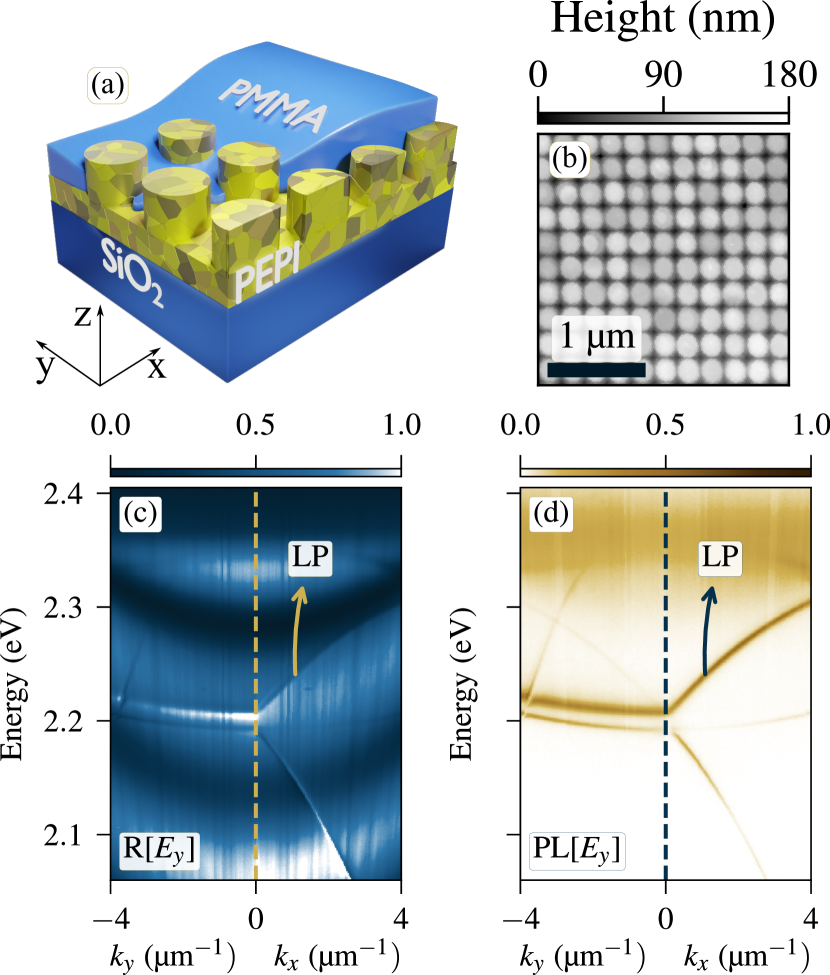
Figure 1: (a) Three-dimensional sketch of the active metasurface studied in this work (not to scale). (b) Scanning electron microscope image of the sample. (c) Reflectivity ($R$) and (d) photoluminescence ($PL$) spectra for $E_{y}$-polarized light with wavevector pointing along the $k_{x}$ and $k_{y}$ directions, respectively, and obtained from the structure pictured in (a). In this paper, our focus lies on the study of the propagation from the lower polariton branch, referred to as “LP” in panels (c)-(d). The broadband signal that is visible in (d) around 2.394 eV is attributed to bare PEPI exciton emission.

Signatures of polariton excitations in the system are experimentally probed by angle-resolved reflectance (ARR) and photoluminescence (ARPL), respectively (we refer to the Methods section for futher details of the experimental setup). For both the ARR and ARPL measurements, the signals can be analyzed in two different polarizations: $E_{y}$ (i.e., S-polarization with respect to $xz$ plane) and $E_{x}$ (i.e., P-polarization with respect to $xz$ plane). In Fig. 1(c,d) we show results for the $E_{y}$ polarization only, along both $k_{x}$ and $k_{y}$. Due to the C₄ symmetry of the square lattice, the results for the $E_{x}$ polarization along $k_{x}$ and $k_{y}$ (not shown here) are identical to those in $E_{y}$ polarization along $k_{y}$ and $k_{x}$, respectively. We now focus on the polariton mode denoted as LP (for Lower Polariton) in Figs. 1(c,d). The strong coupling regime is clearly evidenced by the anticrossing effect observed in both ARR and ARPL spectra. This is highlighted by the bending of the LP mode as it approaches the exciton resonant energy in PEPI ($E_{X}=2.394$ eV). We observe that the dispersion of the LP mode is almost flat along $k_{y}$, but highly dispersive along $k_{x}$, with a relatively large group velocity. Therefore the LP mode is a perfect candidate for studying polariton propagation along the $x$ direction. In addition, as previously discussed, the C₄ symmetry imposes a similar polaritonic mode for the $E_{x}$ polarization, which is the ideal candidate for studying propagation along the $y$ direction.

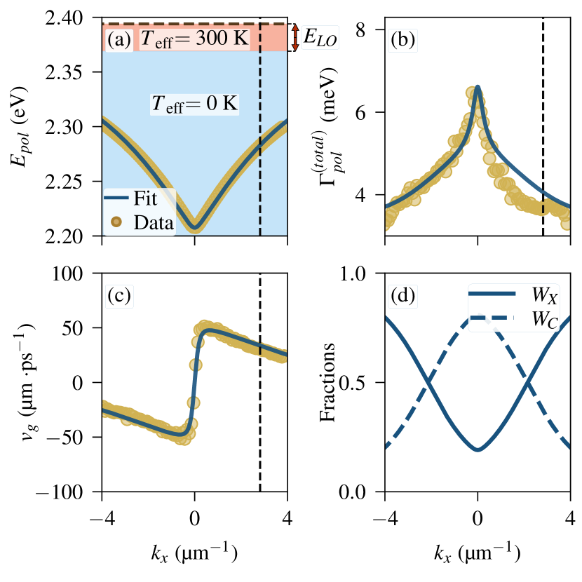
Figure 2: The yellow dots in panels (a), (b) and (c) represent the energy peak position, the linewidth (full width at half maximum), and the group velocity, respectively, measured for the polaritonic branch (LP in Fig. 1), as a function of the wave vector, $k_{x}$. The full lines in (a), (b), and (c) are theoretical curves for the LP polaritonic mode obtained from the coupled oscillators model, with the excitonic resonance indicated as a dashed line in (a). From the same model, we plot in (d) the Hopfield coefficients, the dashed (full) line representing the calculated photonic (excitonic) fraction of this polaritonic mode as a function of the wave vector. In (a,b,c), the vertical dashed lines correspond to the wave vector for which polaritons possess excitonic fraction $W_{X}=63\%$, corresponding to the propagation measurements in Fig. 3 and Fig.4 .

Figures 2(a,b,c) present the resonance energy, linewidth (measured as the full width at half maximum from the PL spectra), and group velocity of LP, extracted from ARPL measurements. The experimental results are nicely fitted by the coupled oscillator model between PEPI excitons and photonic Bloch resonances, given by:

$$\tilde{E}_{pol}(k_{x})=\frac{\tilde{E}_{ph}(k_{x})+\tilde{E}_{X}}{2}-\frac{1}{2}\sqrt{4V^{2}+\left[\tilde{E}_{ph}(k_{x})-\tilde{E}_{X}\right]^{2}}\,.$$ (1)

Here, we can explicitly separate the real part contribution (i.e., the resonances dispersion) from the losses due to the imaginary part: $\tilde{E}_{pol}(k_{x})=E_{pol}(k_{x})+i\Gamma_{pol}(k_{x})/2$. In the expression given in Eq. (1), $V$ is the exciton-photon coupling strength, $\tilde{E}_{X}=E_{X}+i\Gamma_{X}/2$ is the dispersionless excitonic band of energy $E_{X}$ and linewidth $\Gamma_{X}$, and $\tilde{E}_{ph}(k_{x})$ is the complex photonic mode dispersion, which can be approximated by an analytic expression as Eq.(2) (the full expression of all photonic modes along both $k_{x}$ and $k_{y}$ is reported in the Supplemental Information, for completeness):

$$\tilde{E}_{ph}(k_{x})=E_{0}+i\frac{\Gamma_{0}}{2}+\sqrt{\left(\hbar vk_{x}\right)^{2}+\left(U+i\frac{\Gamma_{0}}{2}\right)^{2}}\,.$$ (2)

In Eq. (2), $v$ is the group velocity of the guided modes, which are then folded and coupled by the periodic metasurface. The coupling strength between guided modes is given by the parameter $U$, while $\Gamma_{0}$ accounts for the coupling between guided modes and the radiative continuum, due to the periodic dielectric modulation. From Eq. (2), one may extract the photonic dispersion, $E_{ph}(k_{x})$, as well as the photonic losses, $\Gamma_{ph}(k_{x})$, by calculating the real and imaginary parts of $\tilde{E}_{ph}(k_{x})$, respectively.

The group velocity along $x$ for the given polaritonic branch is straightforwardly obtained from the derivative of real part of the polaritonic dispersion. In the wavevector range shown in Fig. 2(c), the group velocity rapidly increases from $v_{g}=$0\text{\,}\mathrm{\SIUnitSymbolMicro m}\text{\,}{\mathrm{ps}}^{-1}$$ to $v_{g}=$50\text{\,}\mathrm{\SIUnitSymbolMicro m}\text{\,}{\mathrm{ps}}^{-1}$$ for a slight wavevector increase; then, its value remains above $v_{g}=$25\text{\,}\mathrm{\SIUnitSymbolMicro m}\text{\,}{\mathrm{ps}}^{-1}$$ at larger wavevector.

In addition, we report in Fig. 2(d) the calculated Hopfield coefficients (i.e., excitonic and photonic fractions, respectively), given by:

$$W_{X},W_{ph}\approx\frac{1}{2}\left(1\pm\frac{E_{ph}-E_{X}}{\sqrt{(E_{ph}-E_{X})^{2}+4V^{2}}}\right).$$ (3)

Our results demonstrate that perovskite metasurfaces can exhibit highly excitonic polaritons with high group velocity (tens of $\mathrm{\SIUnitSymbolMicro m}\text{\,}{\mathrm{ps}}^{-1}$) and low losses (few $\mathrm{meV}$).

In terms of model parameters, the exciton energy is extracted from the absorption measurement on an unpatterned PEPI thin film, resulting in $E_{X}=$2.394\text{\,}\mathrm{eV}$$. From a fitting procedure, we estimated $E_{0}=$2.294\text{\,}\mathrm{eV}$$, $v=$77.5\text{\,}\mathrm{\SIUnitSymbolMicro m}\text{\,}{\mathrm{ps}}^{-1}$$, $U=$10\text{\,}\mathrm{meV}$$, $\Gamma_{0}=$2.2\text{\,}\mathrm{meV}$$ and $\Gamma_{X}=$0.3\text{\,}\mathrm{meV}$$. The exciton-photon coupling strength is estimated as $V=$127\text{\,}\mathrm{meV}$$, leading to a Rabi-splitting energy of $\sim$254\text{\,}\mathrm{meV}$$ at zero detuning, which is in good agreement with previous reports [37, 38]. An inhomogeneous broadening quantified as $\Gamma_{inh}=$3\text{\,}\mathrm{meV}$$ is added to the total polariton linewidth: $\Gamma_{pol}^{\text{(total)}}=\Gamma_{pol}+\Gamma_{inh}$. Notice that these parameters well reproduce both the real and imaginary parts of the complex LP mode dispersion, as measured from the data shown, e.g., in Figs. 2(a,b,c), as well as from the iso-frequency measurements and propagation experiments in both real and momentum space, that we are going to present in Sec. III.

III Suppression of thermal broadening of perovskite polaritons

Intriguingly, the excitonic losses estimated from the fit in the previous Section, $\Gamma_{X}=0.3$ meV, are orders of magnitude smaller than the value ($\sim$$30\text{\,}\mathrm{meV}$) that is either reported in the literature for the homogeneous linewidth of PEPI excitons at room temperature [33, 34], or obtained from a rough estimate of the full width at half maximum of uncoupled excitons in the PL spectra of Fig. 1(d). Moreover, as shown in Fig. 2(b), the polariton linewidth evidently narrows down as the excitonic fraction increases. As a direct consequence, at $63\%$ excitonic fraction (i.e., $k_{x}\approx$2.8\text{\,}{\mathrm{\SIUnitSymbolMicro m}}^{-1}$$), the measured polariton linewidth is about $4\text{\,}\mathrm{meV}$. Additionally, from the propagation experiment described in the next section, we extract a polariton lifetime of 0.7 ps, corresponding to a homogeneous linewidth of 0.94 meV for polaritonic states with $63\%$ excitonic fraction. This unusual narrowing of the polariton linewidth is explained by the suppression of the thermal broadening for our polaritonic states, as thoroughly described in the following.

In general, exciton-photon interaction is orders of magnitude stronger than exciton-phonon coupling, as explained by Savona and Piermarocchi [39]. Thus, polaritons are primarily formed from photons and “isolated” excitons. Subsequently, the thermal broadening is due to polariton-phonon interaction and not to exciton-phonon interaction. As a consequence, the polariton homogeneous linewidth is given by:

$$\Gamma_{pol}\left(T\right)=\underbrace{W_{C}\cdot\Gamma_{ph}+W_{X}\cdot\Gamma_{X}}_{\text{coupled-oscillator linewidth}}+\Gamma_{\text{th}}\left(T\right)\,,$$ (4)

in which $\Gamma_{X}$ is the homogeneous exciton linewidth at $0\text{\,}\mathrm{K}$ (notice, not at the temperature $T$!), and $\Gamma_{\text{th}}\left(T\right)$ is the thermal broadening induced from the polariton-phonon interaction.

The main contribution to polaritonic dephasing at high-temperature is the optical phonon-polariton interaction, which scatters polaritons into the excitonic states [40, 41, 42]. This process is particularly favourable given the high density of states available in the excitonic reservoir at $E_{X}$. But the energy conservation allows for such scattering in the energy range $E_{pol}\in\left[E_{X}-E_{\text{LO}},E_{X}\right]$, where $E_{\text{LO}}\sim 20-30$ meV is the optical phonons energy in PEPI [43, 33, 34, 44]. This essentially divides the spectrum into two regions, as represented in Fig. 2(a): the first region is defined by $E_{pol}>E_{X}-E_{\text{LO}}$, where polaritons can efficiently scatter with phonons at room temperature; the second region is defined by $E_{pol}<E_{X}-E_{\text{LO}}$, where the phonon-polariton scattering is suppressed and polaritons effectively behave like in an environment at $T_{\text{eff}}=$0\text{\,}\mathrm{K}$$. Strikingly, all the experimental data taken for the LP band are compatible with these polaritons being located in the $T_{\text{eff}}=$0\text{\,}\mathrm{K}$$ region, regardless of the excitonic fraction. Therefore, these polaritons are “cooled” and do not exhibit any thermal broadening: $\Gamma_{th}\approx 0$. This argument gives a remarkably simple but effective account for the reduced polariton linewidth observed in the experimental data reported in Fig. 2(b).

We further notice that the suppression of the polariton-phonon scattering channel was theoretically suggested and experimentally demonstrated by Trichet et al. [40, 41] for ZnO-based polaritons. A similar mechanism was recently predicted for TMD-based polaritons. [42]. In the hypothesis of low losses ($\Gamma_{pol}\ll E_{pol}$, $\Gamma_{X}\ll E_{X}$), the condition $E_{pol}<E_{X}-E_{\text{LO}}$ can be rewritten from Eq.(1) and Eq.(3) as:

$$V>E_{\text{LO}}\sqrt{\frac{W_{X}}{1-W_{X}}}\,.$$ (5)

In particular, for the case of $W_{X}=50\%$, this condition corresponds to $V>E_{\text{LO}}$ [40, 41] that is difficult to be satisfied for exciton-polaritons in III-V semiconductors or TMD monolayers, but it can be easily met in materials with stronger oscillator strengths, such as the PEPI under investigation in the present work. Thus, for PEPI polaritons we can safely assume that $\Gamma_{th}\approx 0$, even for polariton eigenmodes with very large excitonic fraction. Specifically, for our PEPI metasurface, using $V=$127\text{\,}\mathrm{meV}$$ and $E_{\text{LO}}=$30\text{\,}\mathrm{meV}$$, the condition of cooled polaritons Eq.(5) is satisfied for $W_{X}<95\%$.

IV Polariton propagation: measurements in real space

In this section we present the results of a propagation experiment involving polaritonic eigenmodes with $\sim 63\%$ excitonic fraction. From the PL signal under non-resonant pumping, this fraction is selected by using a spectral band-pass filter centered at $E_{f}=$2.283\text{\,}\mathrm{eV}$$. This spectral filtering corresponds to an average wave vector of $2.8\text{\,}{\mathrm{\SIUnitSymbolMicro m}}^{-1}$, with an excitonic fraction of $63\%$.

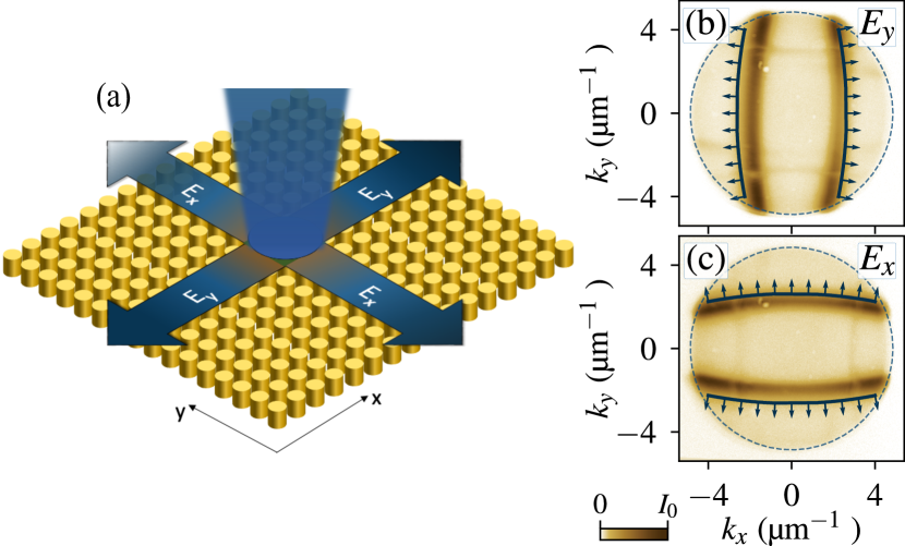
Figure 3: (a) Schematic representation of the in-plane propagation of polaritonic modes excited with $E_{x}$ and $E_{y}$ polarised light, respectively. (b)-(c) Iso-frequency wavevector dispersion of exciton-polaritons, filtered at $E_{0}=$2.283\text{\,}\mathrm{eV}$$, as obtained from mapping the far-field emission in (b) $E_{y}$ and (c) $E_{x}$ polarisations, respectively. The arrows indicate the group velocity patterns. The dashed circles indicate the numerical aperture of the objective lens, while the solid lines are the iso-frequency cuts of the bands calculated with Eq. (1), using the same parameters as in Fig. 2. Details on the theoretical model for the description of polaritonic modes, both as a function of $k_{x}$ and $k_{y}$, are given in the Supplemental Material.

Since the propagation direction is dictated by the group velocity vectors, it is crucial to investigate the group velocity pattern of the polaritons at the selected energy before studying the propagation itself. This pattern can be directly visualized from the iso-frequency mapping of the polaritonic modes. Indeed, the group velocity follows the normal direction of the iso-frequency curves, since it is defined from the gradient of the energy surface in momentum space: $\mathbf{v}_{g}=1/\hbar\,\nabla_{\mathbf{k}}E_{pol}$. Figure 3(b)-(c) presents the measured iso-frequency map for two different polarizations, obtained by projecting the far-field PL emission onto a camera sensor. Two polaritonic modes at this energy are revealed: one is $E_{y}$-polarized, with a dispersion only along $k_{x}$, and corresponding to the LP mode shown in Fig. 1(c)-(d); the other is $E_{x}$-polarized, with dispersion only along $k_{y}$. The results of the iso-frequency curves calculated from the theory are also plotted, showing very good agreement with experimental results. The iso-frequency cuts reveal that the $E_{y}$-($E_{x}$-)polarized mode contains two approximately parallel bands along $k_{y}$ ($k_{x}$), with a group velocity pattern that is almost uniform along the $x$ ($y$) direction. This is further confirmed by the measurement of the group velocity of the LP mode for different values of $k_{y}$, as shown in Fig. S2 of the Supplemental Material.

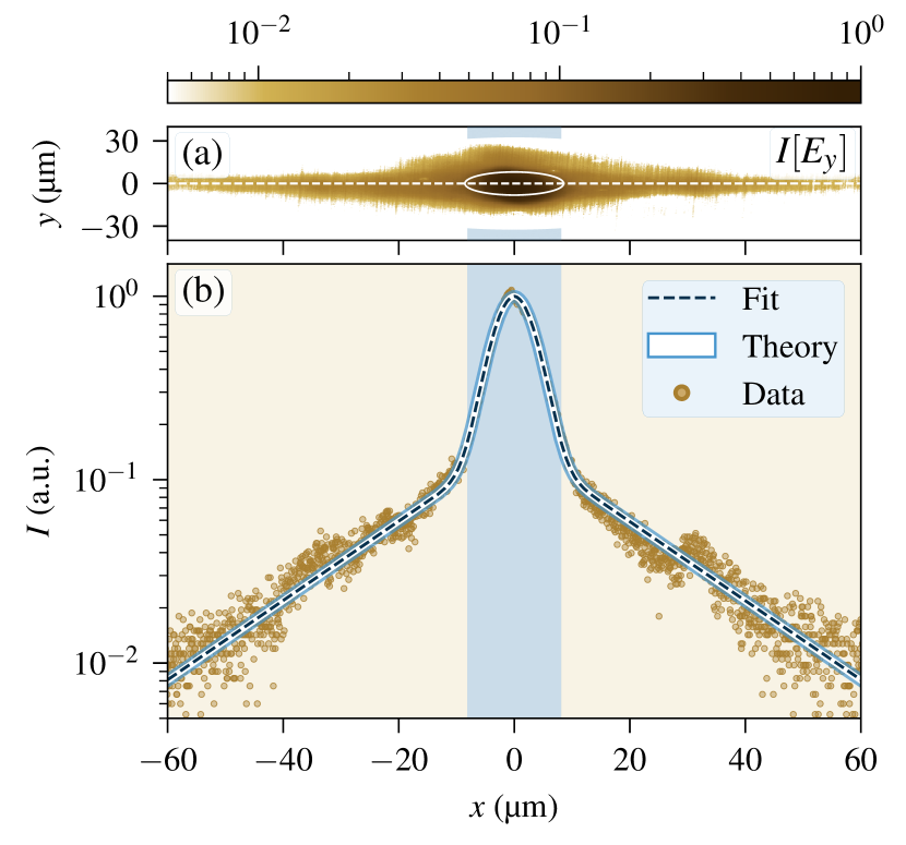
Figure 4: (a) Spatially resolved photoluminescence image of the polaritonic states filtered at $2.283\text{\,}\mathrm{eV}$, with $E_{y}$ polarization selection. The blue-shaded area in the centre corresponds to the pump spot region. (b) Intensity profile selected at $y=0$. The scattered points represent the experimental data, while the dashed line is the fitting results obtained from Eq. (6), and the white line with blue contour is calculated with the theoretical model for the polariton propagation presented in the Supplementary Material.

From the results shown above, we expect that the polariton propagation in the 2D metasurface consists of two one-dimensional flows of uniform propagating fronts with constant group velocity, respectively along the $x$ and $y$ directions, with orthogonal polarizations, as pictorially depicted in Fig. 3(a). Such a propagation scenario is experimentally demonstrated by visualizing the farfield image in real space. In particular, Fig. 4(a) presents the spectrally filtered PL image in real space, measured in $E_{y}$ polarization. In this experiment, the non-resonant pumping of $\sim 2-3$ $\mathrm{\SIUnitSymbolMicro m}$ diameter is focused at $x=y=0$. These results clearly show that polaritons are locally injected at $x=y=0$ under the pump spot, and then propagate along the $x$ direction. Strikingly, the polariton flow remains tightly focused along $y$ direction, even about $x=$60\text{\,}\mathrm{\SIUnitSymbolMicro m}$$ away from the pumping spot, as it is evident from Fig. 4(a). This observation confirms that the velocity vector is aligned along the $x$ direction. Evidently, by switching polarization from $E_{y}$ to $E_{x}$, also the propagation direction switches from $x$ to $y$.

To quantitatively evaluate the propagation properties, the intensity profile at $y=0$ is extracted from the PL image and reported in Fig. 4(b). In the real-space PL, we still have part of the PEPI uncoupled excitonic signal around the excitation spot. Still, these excitons possess high effective mass and zero group velocity, which prevents their propagation over long distances to a large extent. Hence, it is safe to confirm that the PL signal detected far away from the pumping spot comes from propagating polaritons. The PL intensity is then fitted using a phenomenological law of two components function: a Gaussian centered in the origin to account for the excitonic reservoir, an exponential decay curve outside the spot, where the dynamics is dominated by polariton propagation:

$$I(x)=I_{0}e^{-\frac{x^{2}}{2\sigma^{2}}}+I_{1}e^{-\frac{|x|}{l}}\,.$$ (6)

Here, $\sigma$ is the size of the pumping spot and $l$ is the decay length. By applying this function to fit the experimental data, we estimated a propagation constant $l=$20\text{\,}\mathrm{\SIUnitSymbolMicro m}$$ and a pumping spot size $\sigma\sim$3.5\text{\,}\mathrm{\SIUnitSymbolMicro m}$$. This value of decay length corresponds to a polariton lifetime of $0.7\text{\,}\mathrm{ps}$, if ballistic propagation is assumed. This lifetime corresponds to a homogeneous linewidth of $0.94\text{\,}\mathrm{meV}$. We notice that this linewidth is much smaller than the value $4\text{\,}\mathrm{meV}$ obtained from the fit in the previous section. This indicates that the inhomogeneous broadening effects are the dominant contributions to the total polariton linewidth in the emission spectra. Such an observation is in good agreement with the value $\Gamma_{inh}=3$ meV, which is used as fitting parameter for the inhomogeneous broadening in the results of Fig. 2. Finally, the same parameters for the polaritonic modes are implemented in a 1D propagation model (see the Supplemental Material for details). The calculated spatial decay given by this model, whose results are shown in Fig. 4, perfectly reproduces the experimental results and the phenomenological law.

V Polariton propagation: measurements in momentum space

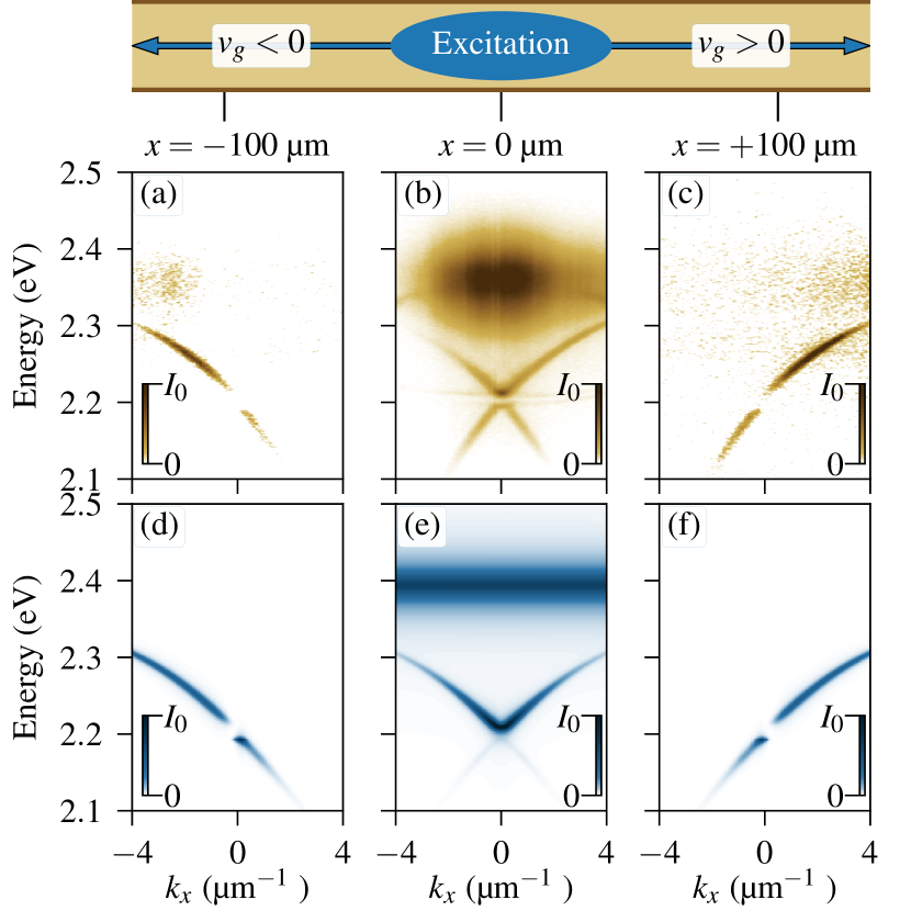
Figure 5: (a)-(b)-(c) Normalized PL spectra obtained by spatially filtering the signal at $x=$-100\text{\,}\mathrm{\SIUnitSymbolMicro m}$$, $x=$0\text{\,}\mathrm{\SIUnitSymbolMicro m}$$ and $x=$100\text{\,}\mathrm{\SIUnitSymbolMicro m}$$, respectively. The pump spot is focused at $x=$0\text{\,}\mathrm{\SIUnitSymbolMicro m}$$. (d)-(e)-(f) Simulated PL spectra calculated for the same positions as (a)-(b)-(c). Details on the theoretical model for the description of polariton propagation, as well as on the signal denoising, are given in the Supplemental Material.

To investigate the ballistic nature of the polariton propagation in the nano-imprinted 2D metasurfaces, we show the monitoring of this propagation in momentum space, with the aim of probing possible backscattering. To do so, a slit of width $S=$17\text{\,}\mathrm{\SIUnitSymbolMicro m}$$, playing the role of a spatial filter, is put at the intermediate image position in the optical path of the ARPL experiment setup [45]. By moving the slit position along the $x-$axis, we can probe the polariton dispersion either immediately below or far from the excitation spot. In this experiment, the spectral filter from the previous experiment is removed. The experimental results corresponding to three different slit positions are shown in Fig. 5(a-c). The corresponding theoretical calculations, obtained from the 1D propagation model, are shown in Fig 5(d-e).

Under the pumping spot at $x=0$, the ARPL results show all of the polaritonic branches that were previously visible in the measured reflectivity and PL spectra of Fig. 1(c)-(d). We notice that all the branches reported in Fig. 5 are broadened as compared to the ones measured without spatial filter in Fig. 1(c)-(d). This is due to an uncertainty on the emission wavevector, $\Delta_{k}\approx 1/S$, introduced by the finite extent of the spatial filter. Moreover, the intensity distribution is very different from the one measured without the spatial filter: the strongest signals are observed from the uncoupled excitons and the zero-group velocity point in the polariton branches. Indeed, polaritons/excitons injected in these states cannot propagate, and would radiatively emit photoluminescence under the pump spot, while states of non-zero group velocity propagate out of the pump spot region.

At $x=$100\text{\,}\mathrm{\SIUnitSymbolMicro m}$$ ($x=-$100\text{\,}\mathrm{\SIUnitSymbolMicro m}$$) away from the excitation, only polaritonic states at positive (negative) group velocity are observed. This demonstrates that polaritons propagate ballistically along the $x$ direction without any backscattering. Moreover, thanks to the absence of the signal from uncoupled excitons far from the pump spot, we can appreciate the linewidth narrowing of the LP branch when it approaches the excitonic energy. This appears as a further confirmation of our interpretation about the quenching of the thermal broadening. Most impressively, this propagation across $100\text{\,}\mathrm{\SIUnitSymbolMicro m}$ is observed even with polaritons at $k_{x}=$4\text{\,}{\mathrm{\SIUnitSymbolMicro m}}^{-1}$$, corresponding to an excitonic fraction of 80$\%$. Since the extracted lifetime for polaritonic eigenmodes with $55\%$ excitonic fraction is $0.7\text{\,}\mathrm{ps}$, which is only limited by the photonic losses, we estimate that the lifetime of these 80$\%$ excitonic fraction polaritons is even longer, about $1.26\text{\,}\mathrm{ps}$.

VI Conclusion and Perspectives

We have successfully demonstrated ballistic propagation, in the hundred-micrometer-range, of high-excitonic-fraction polaritons at room temperature. This significant achievement is enabled by the suppression of thermal-induced broadening in perovskite polaritons, formed within a large-scale and homogeneous perovskite metasurface fabricated through direct nano-imprint technology. The metasurface design introduces an innovative mechanism for directing unidirectional and high-speed propagation across macroscopic distances through polarization control. Given the strong nonlinearity exhibited by PEPI polaritons at high excitonic fractions [46], our platform opens new avenues for exploring nonlinear transport of quantum fluids of light beyond traditional microcavity architectures. By leveraging methods such as the precise tailoring photonic dispersion [47], or employing novel concepts of loss engineering such as bound states in the continuum [48, 49, 50], we anticipate unlocking new regimes of superfluidity and non-equilibrium hydrodynamics. Finally, from the potential applications perspective, the ability to route and confine low-loss, highly nonlinear polaritons at room temperature using a scalable and cost-effective fabrication method paves the way for integrating polariton physics into all-optical and integrated devices, marking a significant advancement for the field where polariton-based devices could revolutionize signal processing and transmission.

Acknowledgement: The authors would like to thank the staff from the Nanolyon Technical Platform for helping and supporting all nanofabrication processes. We also thank Le Si Dang and Lucio Claudio Andreani for fruitful discussions. H.S.N, C.S, E.D acknowledge financial support from by the French National Research Agency (ANR) under the project POPEYE (ANR-17-CE24-0020), project EMIPERO (ANR-18-CE24-0016). S.Z. and D.G. acknowledge financial support from PNRR MUR project PE0000023-NQSTI.

VII METHODS

VII.1 Sample fabrication

The fabrication process initiates by depositing a thin layer of PEPI onto substrates composed of $2\text{\,}\mathrm{\SIUnitSymbolMicro m}$ thick SiO₂ on silicon (Si). This is achieved by spin-coating a 20% wet solution of PEPI in Dimethylformamide (DMF) at 5000 rpm for 30 seconds. Following this step, the PEPI film undergoes annealing at 95°C for 90 seconds to induce crystallization before proceeding to the imprinting step. Subsequently, a Si mold with the desired structure is pressed onto the PEPI film using a thermal press. This imprinting process occurs at 100°C under a pressure of 100 bar for approximately 10 minutes. As a result, the structure from the mold is directly transferred onto the PEPI film. Details of the fabrication method were already reported in Ref.  [36].

VII.2 Experimental setup

The sample is illuminated via a microscope objective (20x magnification, NA=0.42) using a white-light beam (halogen lamp) for ARR experiments or a non-resonant laser ($400\text{\,}\mathrm{nm}$, $80\text{\,}\mathrm{MHz}$, $50\text{\,}\mathrm{ps}$) for ARPL experiments . The signal that is scattered or emitted from the sample is then collected through the same objective, and analyzed by imaging the back-focal plane of the microscope objective for measurements in momentum-space, or the sample plane for measurements in real-space. For dispersion measurements, the signal is first projected onto the entrance of a spectrometer, whose output is coupled to the sensor of a CCD camera. For the propagation experiment in real-space, the signal is spectrally filtered by a band pass filter at 543 nm, and then projected onto the sensor of a SCMOS camera. For the propagation experiment in momentum space, the signal is spatially filtered by a slit that is positioned in correspondence of the plane of the intermediate image [45].

I Suppression of thermal broadening

In order to investigate the impact of exciton losses on the polariton, we performed the fit of Eq. (1) reported in the main text in two different configurations. In the first case, we fixed the excitonic linewidth at $\Gamma_{X}=$0.3\text{\,}\mathrm{meV}$$, representing excitonic losses without any thermal broadening effect. Secondly, we set the exciton linewidth corresponding to the bare exciton as $\Gamma_{X}=$30\text{\,}\mathrm{meV}$$, i.e., including thermal broadening effects. The resulting polaritonic linewidths are compared in Fig. S1 with experimental data extracted from the photoluminescence (PL) spectrum of Fig. 1(d) in the main text. Remarkably, we observed a significant agreement between the fitted model and experimental results for the choice $\Gamma_{X}=$0.3\text{\,}\mathrm{meV}$$, meaning that polariton losses are not affected by thermal broadening of the bare excitons.

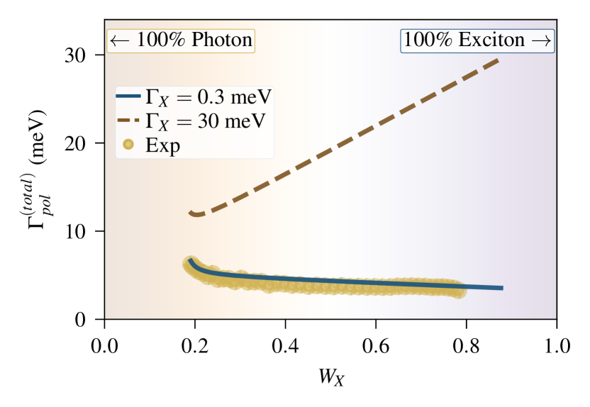
Figure S1: The lines depict the polaritonic linewidths for various excitonic fractions $W_{X}$, as fitted from Eq. (1) in the main text. The solid line represents the fit with an excitonic linewidth $\Gamma_{X}=$0.3\text{\,}\mathrm{meV}$$, while the dashed line corresponds to $\Gamma_{X}=$30\text{\,}\mathrm{meV}$$. Scattered data points are derived from experimental PL measurements.

II Measurement of the group velocity pattern for 63$\%$ excitonic-fraction polaritons

With the aim of highlighting the uniform group velocity along $x$-direction for $y$-polarized polaritons in the 63$\%$ excitonic fraction case, we experimentally measured the group velocity, $v_{g}$, corresponding to different values of $k_{y}$. Here, the velocity is extracted from the slope of the dispersion along $k_{x}$, at various values of $k_{y}$. Experimentally, the scanning of $k_{y}$ is achieved by moving the image of the back-focal plane of the microscope objective with respect to the entrance slit of the spectrometer [45]. The results, shown in Fig. S2(a), confirm that the group velocity (for both forward and backward propagating polaritons) does not depend on $k_{y}$.

Moreover, we can also extract the polariton linewidth, $\Gamma_{pol}$, at different values of $k_{y}$ from the very same measurements. The results, shown in Fig. S2(b), confirm that the polariton linewidth does not depend on $k_{y}$, as predicted by the analytical model.

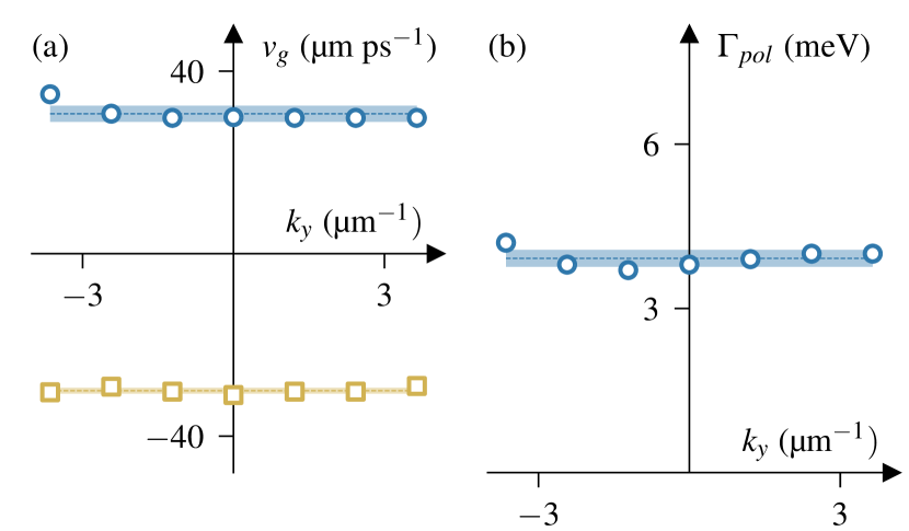
Figure S2: Experimental results for (a) the group velocity along $x$ direction, and (b) the linewidth of $y$-polarized polaritons having 63$\%$ excitonic fraction. The colored areas represent 1 standard deviation around the average values.

III Theoretical model for photonic and polaritonic dispersions

III.1 Photonic modes

As discussed in detail in Ref. [36], the two photonic modes that give rise to the two polaritonic branches observed in Figs. 1(c,d) can be described by the following analytic expression:

$$\tilde{E}_{ph(\pm)}=E_{0}+i\frac{\Gamma_{0}}{2}\pm\sqrt{\left(\hbar vk_{x}\right)^{2}+\left(U+i\frac{\Gamma_{0}}{2}\right)^{2}}+\frac{\hbar va}{4\pi}k_{y}^{2}\,,$$ (S1)

in which $v$ is the group velocity of the photonic guided modes that are folded and coupled by the periodic metasurface with lattice pitch $a$. The coupling strength between guided modes is quantified by the parameter $U$, while $\Gamma_{0}$ accounts for the coupling between guided modes and the radiative continuum, due to the periodic dielectric modulation. From this expression, we separate the real part contribution (i.e., the resonances dispersion) from the the imaginary part (i.e., the contribution to the losses):

$$\tilde{E}_{ph(\pm)}=E_{ph(\pm)}+i\frac{\Gamma_{ph(\pm)}}{2}\,.$$ (S2)

Notice that the $\tilde{E}_{ph+}$ photonic mode in the latter expression corresponds to the mode indicated as $\tilde{E}_{ph}$ in Eq. (2) of the main text.

III.2 Strong coupling regime

The coupling between these photonic modes and perovskite excitons gives rise to four polartonic branches [36], analytically described as:

$$\tilde{E}_{LP(\pm)} =\frac{\tilde{E}_{ph(\pm)}+\tilde{E}_{X}}{2}-\sqrt{V^{2}+\left[\frac{\tilde{E}_{ph(\pm)}-\tilde{E}_{X}}{2}\right]^{2}}\,,$$ (S3)

$$\tilde{E}_{UP(\pm)} =\frac{\tilde{E}_{ph(\pm)}+\tilde{E}_{X}}{2}+\sqrt{V^{2}+\left[\frac{\tilde{E}_{ph(\pm)}-\tilde{E}_{X}}{2}\right]^{2}}\,,$$ (S4)

from which the decomposition into real and imaginary parts can be explicitly written as:

$$\tilde{E}_{LP(\pm)} =E_{LP(\pm)}+i\frac{\Gamma_{LP(\pm)}}{2}\,,$$ (S5)

$$\tilde{E}_{UP(\pm)} =E_{UP(\pm)}+i\frac{\Gamma_{UP(\pm)}}{2}\,.$$ (S6)

Also in this case, notice that the polaritonic mode here indicated as $\tilde{E}_{LP+}$ corresponds to the one denoted as $\tilde{E}_{pol}$ in Eq. (1) of the main text. The calculated dispersion and linewidth of photonic modes and lower polaritonic modes, obtained from Eq. (S1) and Eq. (S3), are presented in Fig. S3. The model parameters used to obtain the results for these plots read as follows: $a=$300\text{\,}\mathrm{nm}$$, $v=$77.5\text{\,}\mathrm{\SIUnitSymbolMicro m}\text{/}\mathrm{ps}$$, $U=$10\text{\,}\mathrm{meV}$$, $\Gamma_{0}=$2.2\text{\,}\mathrm{meV}$$, $E_{X}=$2.394\text{\,}\mathrm{eV}$$, $E_{0}=$2.294\text{\,}\mathrm{eV}$$ and $\Gamma_{X}=$0.3\text{\,}\mathrm{meV}$$. Finally, to take into account the effect of disorder, an inhomogeneous broadening of $\Gamma_{inh}=3$ meV is added to the polariton linewidths, such that:

$$\Gamma_{LP(\pm)}^{\text{(total)}} =\Gamma_{LP(\pm)}+\Gamma_{inh}\,,$$ (S7)

$$\Gamma_{UP(\pm)}^{\text{(total)}} =\Gamma_{UP(\pm)}+\Gamma_{inh}\,.$$ (S8)

As shown in the main text, we obtain an almost perfect matching between experimental data and the analytic curves obtained from this model, both for the real and imaginary parts of polaritonic modes, respectively.

III.3 iso-frequency curves in high momentum limit

In the limit of a large momentum, $\hbar vk_{x}\gg U,\Gamma_{0}$, the expressions for the photonic modes given in Eq. Eq. (S1) simplify as:

$$\tilde{E}_{ph(\pm)}\approx E_{0}+i\frac{\Gamma_{0}}{2}\pm\hbar vk_{x}+\frac{\hbar va}{4\pi}k_{y}^{2}\,.$$ (S9)

Moreover, considering that the losses $\Gamma_{0}$,$\Gamma_{X}$ are negligeable with respect to $\hbar vk_{x}$ and $V$, the real part dispersion of the lower polariton modes, given by Eq. (S3), can be rewritten as:

$$E_{LP(\pm)}\approx\frac{E_{0}+E_{X}}{2}\pm\frac{\hbar vk_{x}}{2}+\frac{\hbar va}{8\pi}k_{y}^{2}-\sqrt{V^{2}+\left[\frac{E_{0}-E_{X}}{2}\pm\frac{\hbar vk_{x}}{2}+\frac{\hbar va}{8\pi}k_{y}^{2}\right]^{2}}\,.\\$$ (S10)

We notice that the expressions above are for polaritonic modes coming from $E_{y}$-polarized photonic branches. For polaritonic modes arising from $E_{x}$-polarized photons, we will have similar expression but switching between $k_{x}$ and $k_{y}$. Therefore, the iso-frequency curves at $E_{iso}$ for $LP(+)$ modes are given by:

$$\frac{\hbar vk_{x}}{2}+\frac{\hbar va}{8\pi}k_{y}^{2}-\sqrt{V^{2}+\left[\frac{E_{0}-E_{X}}{2}+\frac{\hbar vk_{x}}{2}+\frac{\hbar va}{8\pi}k_{y}^{2}\right]^{2}}+\frac{E_{0}+E_{X}}{2}-E_{iso} =0\,,$$ (S11)

$$\frac{\hbar vk_{y}}{2}+\frac{\hbar va}{8\pi}k_{x}^{2}-\sqrt{V^{2}+\left[\frac{E_{0}-E_{X}}{2}+\frac{\hbar vk_{y}}{2}+\frac{\hbar va}{8\pi}k_{x}^{2}\right]^{2}}+\frac{E_{0}+E_{X}}{2}-E_{iso} =0\,$$ (S12)

for $E_{y}$ and $E_{x}$ polarization respectively.

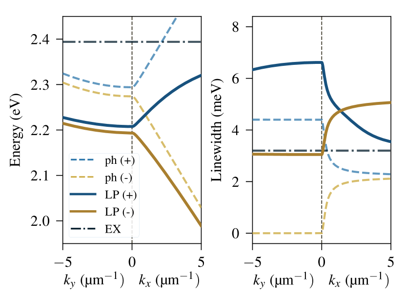
Figure S3: Theoretical calculation of the (a) energy dispersion and (b) linewidth along $k_{x}$ and $k_{y}$ of photonic modes $\tilde{E}_{ph(\pm)}$ and lower polaritonic modes $\tilde{E}_{LP(\pm)}$ that are given by Eq. (S1) and Eq. (S3) , respectively. The parameters are: $a=$300\text{\,}\mathrm{nm}$$, $v=$77.5\text{\,}\mathrm{\SIUnitSymbolMicro m}\text{/}\mathrm{ps}$$, $U=$10\text{\,}\mathrm{meV}$$, $\Gamma_{0}=$2.2\text{\,}\mathrm{meV}$$, $E_{X}=$2.394\text{\,}\mathrm{eV}$$, $E_{0}=$2.294\text{\,}\mathrm{eV}$$, $\Gamma_{X}=$0.3\text{\,}\mathrm{meV}$$ and $\Gamma_{inh}=3$ meV

.

IV Theoretical model for polariton propagation

In this section, we present the theoretical model corresponding to the results shown in Figs. 5(d,e,f) of the main text.

IV.1 Polariton density

In order to study the propagation of polaritonic excitations within the metasurface plane, we developed an approximated method to calculate the steady state spatial density distribution of polaritons with complex energy dispersion $\tilde{E}_{pol}=E_{pol}+i\Gamma_{pol}/2$, defined as $n(x,\tilde{E}_{pol})$. The input parameters of the model are given in the previous Sec. III. We discuss only the case of $y-$polarised polaritons here, while the case of $x-$polarised polaritons can be easily derived from the former. In the case of $y-$polarised polaritons, the propagation can be well approximated by a group velocity pointing in the $x$ direction, $\mathbf{v}_{g}=v_{g}\hat{x}$, where $\hat{x}$ is the unit vector of the $x$ coordinate axis. This assumption is justified from the energy cut shown in Fig. 3(a). We start by considering a generation rate $G(x,E_{pol})$ for polaritons with energy $E_{pol}$ at position $x$, as obtained from a non-resonant Gaussian excitation spot centered at $x=0$, i.e.,

$$G(x,E_{pol})=G_{0}(E_{pol})e^{-x^{2}/2\sigma^{2}}\,,$$ (S13)

in which the amplitude $G_{0}(E_{pol})$ represents the spectral distribution of polariton injection, and $\sigma$ determines the spot size. For a given polariton energy $E_{pol}$, a polaritonic mode has a well defined group velocity $v_{g}$. On a first approximation, we can neglect any nonlinear effect, i.e., we assume that each energy component of the polaritonic dispersion is independent from the others. In steady state, the total net flux of polaritons is null, and we get the condition:

$$\frac{\partial n(x,\tilde{E}_{pol})}{\partial x}v_{g}+\Gamma_{pol}n(x,\tilde{E}_{pol})=G(x,E_{pol})\,.$$ (S14)

Using the generation rate obtained from Eq. (S13), we have the differential equation:

$$\frac{\partial n(x,\tilde{E}_{pol})}{\partial x}v_{g}+\Gamma_{pol}n(x,\tilde{E}_{pol})=G_{0}(E_{pol})e^{-x^{2}/2\sigma^{2}}.$$ (S15)

At $x=0$, the polariton density is maximized for any eigenmode of energy $E_{pol}$, thus $\frac{\partial n(0,\tilde{E}_{pol})}{\partial x}=0$, which gives the boundary condition:

$$n(0,\tilde{E}_{pol})=\frac{G_{0}(E_{pol})}{\Gamma_{pol}}\,.$$ (S16)

Moreover, for each polariton eigenmode with complex energy $\tilde{E}_{pol}$, using Eq. (S16) as initial value at $x=0$, Eq. (S15) can be easily integrated numerically, which gives the solution $n(x,\tilde{E}_{\text{pol}})$ of the polariton density.

We finally notice that the same excitation spot is also responsible for the injection of non-propagating uncoupled excitons with density:

$$n_{X}(x)=n_{0}e^{-x^{2}/2\sigma^{2}}\,.$$ (S17)

IV.2 The PL signal

The photoluminesce (PL) spectrum measured at energy $E$ and due to a polariton eigenmode with complex energy $\tilde{E}_{pol}=E_{pol}+i\Gamma_{pol}/2$ can be modeled by the following Lorentzian profile:

$$S_{pol}(E,\tilde{E}_{pol})=\frac{(\Gamma_{pol}+\Gamma_{inh})}{\pi\left[(E-E_{pol})^{2}+(\Gamma_{pol}+\Gamma_{inh})^{2}/4\right]}\,.$$ (S18)

The PL intensity of the polariton mode at energy $E_{pol}$, when spatially selected at position $x\in[x_{1},x_{2}]$, is given by:

$$I_{pol}(E,\tilde{E}_{pol})\propto\underbrace{S_{pol}(E,\tilde{E}_{pol})}_{\text{spectrum}}.\underbrace{(\Gamma_{pol}-W_{X}.\Gamma_{X})}_{\text{radiative losses}}.\underbrace{\int_{x_{1}}^{x_{2}}n(x,\tilde{E}_{pol})dx}_{\text{polariton population}}.$$ (S19)

Similarly, the PL spectrum and the PL intensity of uncoupled excitons, when spatially selected in position $x\in[x_{1},x_{2}]$, are respectively given by:

$$S_{X}(E) =\frac{\Gamma_{X}^{\text{(uncoupled)}}}{\pi\left[(E-E_{X})^{2}+\left(\Gamma_{X}^{\text{(uncoupled)}}\right)^{2}/4\right]}$$ (S20)

$$I_{X}(E) \propto S_{X}(E)\int_{x_{1}}^{x_{2}}n_{X}(x)dx\,.$$ (S21)

Here, the linewidth $\Gamma_{X}^{\text{(uncoupled)}}$ of uncoupled excitons is the room temperature one, i.e., including thermal broadening effects, and thus $\Gamma_{X}^{\text{(uncoupled)}}=30$ meV.

Taking into account the two lower polaritonic branches, $LP(\pm)$, and the uncoupled excitons, the total PL intensity at energy $E$ and wavevector $k_{x}$, when spatially selected at position $x\in[x_{1},x_{2}]$, is given by:

$$I_{total}(E,k_{x})=\sum_{pol=LP(\pm)}I_{pol}\left(E,\tilde{E}_{pol}(k_{x})\right)+I_{X}(E)\,,$$ (S22)

in which $E_{LP(\pm)}(k_{x})$ represent the dispersions of the lower polariton modes, respectively, as given in Eq. (S3). Finally, a selection in real space (i.e., spatial selection) induces a broadening in momentum space, due to the reciprocal relation $\Delta_{x}\cdot\Delta_{k}\sim 1$. This broadening is taken into account by a convolution of $I_{total}(E,k_{x})$ with a Gaussian function whose standard deviation is $\Delta_{k}$.

IV.3 Numerical parameters

The dependence of the polariton energy on the wave-vector along the propagation direction, $E_{pol}(k_{x})$, and its corresponding linewidth, $\Gamma_{pol}(k_{x})$, is calculated as detailed in Sec. III, for both polaritonic eigenmodes. The only supplemental parameters to calculate the spatial distribution of polariton density [see Eq. (S14)] and the PL in momentum space [see Eq. (S22)] are the spectral distribution $G_{0}(E_{pol})$ for the polariton injection, and the injection density $n_{0}$ for uncoupled excitons. For the former, we apply a simple phenomenological law, i.e., assuming $G_{0}(E_{pol})\propto\exp\left(-|E_{pol}-E_{c}|/W\right)$, which exhibits a polariton concentration at energy $E_{c}$. Numerically, we assume $W=$30\text{\,}\mathrm{meV}$$, $E_{c}=$2.209\text{\,}\mathrm{eV}$$ for LP(+) mode and $E_{bn}=$2.17\text{\,}\mathrm{eV}$$ for LP(-) mode. For the amplitude of injection, we assume that the LP(+) mode is pumped 80 times more efficiently than the LP(-) one. Using these parameters, the theoretical calculation for the decay of 63$\%$ excitonic-fraction polaritons in real-space, as well as the polariton density in momentum-space after spatial selection, are presented in Fig. 4 in the main text. We highlight the remarkably good agreement between these calculation and the experimental data presented in Figs. 4 and 5 of the main text.

V Denoising of PL signal

Figure S4: $S_{1}$, $S_{2}$, and $S_{3}$ are three PL signals coming from three different positions on the sample. These signals are then convoluted using the kernel $K$ defined in Eq. (S23), and reported in the plot as $S_{1}\ast K$, $S_{2}\ast K$ and $S_{3}\ast K$. These convoluted signals are the ones also reported in Fig. 5(a-c) of the main text.

The signal-to-noise ratio of propagated polaritons in Fig. 5(a-c) is particularly low. This is due to the signal collection being performed at $|x|=$100\text{\,}\mathrm{\SIUnitSymbolMicro m}$$ from the excitation spot, while the propagation length fitted from Fig. 4 is estimated to be of the order of $l\approx$20\text{\,}\mathrm{\SIUnitSymbolMicro m}$$. To “denoise” the experimental data of Fig. 5(a-c), we performed a convolution $S\ast K$ of the signal $S$ using a $5\times 5$ Gaussian kernel $K$ defined as:

$$K=\frac{1}{2^{8}}\begin{bmatrix}1&4&6&4&1\\ 4&16&24&16&4\\ 6&24&36&24&6\\ 4&16&24&16&4\\ 1&4&6&4&1\end{bmatrix}\,.$$ (S23)

The convolution kernel in Eq. (S23) is normalized such that the sum of all its elements is equal to 1. Since the Fourier transform of a Gaussian is still a Gaussian, the convolution between the actual signal and $K$ quenches the high-frequency components. The low-pass filtering effect of such a convolution effectively increases the signal-to-noise ratio. As an example, this is explicitly demonstrated in Fig. S4, in which we show three the signals obtained from PL measurements before (upper panels) and after (lower panels) the convolution. The same convolution technique has been used to denoise the experimental data shown in Fig. 3 in the main text.

References

- Hopfield [1958] J. J. Hopfield, Theory of the contribution of excitons to the complex dielectric constant of crystals, Phys. Rev. 112, 1555 (1958).
- Agranovich [1960] V. M. Agranovich, Dispersion of electromagnetic waves in crystals, Sov. Phys. JETP 37, 307 (1960).
- Weisbuch et al. [1992] C. Weisbuch, M. Nishioka, A. Ishikawa, and Y. Arakawa, Observation of the coupled exciton-photon mode splitting in a semiconductor quantum microcavity, Phys. Rev. Lett. 69, 3314 (1992).
- Carusotto and Ciuti [2013] I. Carusotto and C. Ciuti, Quantum fluids of light, Rev. Mod. Phys. 85, 299 (2013).
- Sanvitto and Kéna-Cohen [2016] D. Sanvitto and S. Kéna-Cohen, The road towards polaritonic devices, Nature Materials 15, 1061–1073 (2016).
- Gao et al. [2012] T. Gao, P. S. Eldridge, T. C. H. Liew, S. I. Tsintzos, G. Stavrinidis, G. Deligeorgis, Z. Hatzopoulos, and P. G. Savvidis, Polariton condensate transistor switch, Phys. Rev. B 85, 235102 (2012).
- Ballarini et al. [2013a] D. Ballarini, M. De Giorgi, E. Cancellieri, R. Houdré, E. Giacobino, R. Cingolani, A. Bramati, G. Gigli, and D. Sanvitto, All-optical polariton transistor, Nature Communications 4, 10.1038/ncomms2734 (2013a).
- Amo et al. [2011] A. Amo, S. Pigeon, D. Sanvitto, V. G. Sala, R. Hivet, I. Carusotto, F. Pisanello, G. Leménager, R. Houdré, E. Giacobino, C. Ciuti, and A. Bramati, Polariton superfluids reveal quantum hydrodynamic solitons, Science 332, 1167 (2011).
- Nguyen et al. [2013] H. S. Nguyen, D. Vishnevsky, C. Sturm, D. Tanese, D. Solnyshkov, E. Galopin, A. Lemaître, I. Sagnes, A. Amo, G. Malpuech, and J. Bloch, Realization of a double-barrier resonant tunneling diode for cavity polaritons, Phys. Rev. Lett. 110, 236601 (2013).
- Amo et al. [2009] A. Amo, J. Lefrère, S. Pigeon, C. Adrados, C. Ciuti, I. Carusotto, R. Houdré, E. Giacobino, and A. Bramati, Superfluidity of polaritons in semiconductor microcavities, Nature Physics 5, 805 (2009).
- Nguyen et al. [2015] H. S. Nguyen, D. Gerace, I. Carusotto, D. Sanvitto, E. Galopin, A. Lemaître, I. Sagnes, J. Bloch, and A. Amo, Acoustic black hole in a stationary hydrodynamic flow of microcavity polaritons, Phys. Rev. Lett. 114, 036402 (2015).
- Lerario et al. [2016] G. Lerario, D. Ballarini, A. Fieramosca, A. Cannavale, A. Genco, F. Mangione, S. Gambino, L. Dominici, M. D. Giorgi, G. Gigli, and D. Sanvitto, High-speed flow of interacting organic polaritons, Light: Science Applications 6, e16212 (2016).
- Liran et al. [2018] D. Liran, I. Rosenberg, K. West, L. Pfeiffer, and R. Rapaport, Fully guided electrically controlled exciton polaritons, ACS Photonics 5, 4249 (2018).
- Wertz et al. [2010] E. Wertz, L. Ferrier, D. D. Solnyshkov, R. Johne, D. Sanvitto, A. Lemaître, I. Sagnes, R. Grousson, A. V. Kavokin, P. Senellart, G. Malpuech, and J. Bloch, Spontaneous formation and optical manipulation of extended polariton condensates, Nature Physics 6, 860 (2010).
- Steger et al. [2013] M. Steger, G. Liu, B. Nelsen, C. Gautham, D. W. Snoke, R. Balili, L. Pfeiffer, and K. West, Long-range ballistic motion and coherent flow of long-lifetime polaritons, Phys. Rev. B 88, 235314 (2013).
- Freixanet et al. [2000] T. Freixanet, B. Sermage, A. Tiberj, and R. Planel, In-plane propagation of excitonic cavity polaritons, Phys. Rev. B 61, 7233 (2000).
- Langbein et al. [2007] W. Langbein, I. Shelykh, D. Solnyshkov, G. Malpuech, Y. Rubo, and A. Kavokin, Polarization beats in ballistic propagation of exciton-polaritons in microcavities, Phys. Rev. B 75, 075323 (2007).
- Suárez-Forero et al. [2020] D. G. Suárez-Forero, V. Ardizzone, S. F. C. da Silva, M. Reindl, A. Fieramosca, L. Polimeno, M. D. Giorgi, L. Dominici, L. N. Pfeiffer, G. Gigli, D. Ballarini, F. Laussy, A. Rastelli, and D. Sanvitto, Quantum hydrodynamics of a single particle, Light: Science Applications 9, 10.1038/s41377-020-0324-x (2020).
- Walker et al. [2013] P. M. Walker, L. Tinkler, M. Durska, D. M. Whittaker, I. J. Luxmoore, B. Royall, D. N. Krizhanovskii, M. S. Skolnick, I. Farrer, and D. A. Ritchie, Exciton polaritons in semiconductor waveguides, Applied Physics Letters 102, 012109 (2013).
- Marsault et al. [2015] F. Marsault, H. S. Nguyen, D. Tanese, A. Lemaître, E. Galopin, I. Sagnes, A. Amo, and J. Bloch, Realization of an all optical exciton-polariton router, Applied Physics Letters 107, 201115 (2015).
- Ballarini et al. [2013b] D. Ballarini, M. D. Giorgi, E. Cancellieri, R. Houdré, E. Giacobino, R. Cingolani, A. Bramati, G. Gigli, and D. Sanvitto, All-optical polariton transistor, Nature Communications 4, 10.1038/ncomms2734 (2013b).
- Franke et al. [2012] H. Franke, C. Sturm, R. Schmidt-Grund, G. Wagner, and M. Grundmann, Ballistic propagation of exciton–polariton condensates in a ZnO-based microcavity, New Journal of Physics 14, 013037 (2012).
- Hou et al. [2020] S. Hou, M. Khatoniar, K. Ding, Y. Qu, A. Napolov, V. M. Menon, and S. R. Forrest, Ultralong-range energy transport in a disordered organic semiconductor at room temperature via coherent exciton-polariton propagation, Advanced Materials 32, 2002127 (2020).
- Zhang et al. [2011] C. Zhang, C.-L. Zou, Y. Yan, R. Hao, F.-W. Sun, Z.-F. Han, Y. S. Zhao, and J. Yao, Two-photon pumped lasing in single-crystal organic nanowire exciton polariton resonators, Journal of the American Chemical Society 133, 7276 (2011).
- Ciers et al. [2017] J. Ciers, J. G. Roch, J.-F. Carlin, G. Jacopin, R. Butté, and N. Grandjean, Propagating polaritons in iii-nitride slab waveguides, Phys. Rev. Appl. 7, 034019 (2017).
- Barachati et al. [2018] F. Barachati, A. Fieramosca, S. Hafezian, J. Gu, B. Chakraborty, D. Ballarini, L. Martinu, V. Menon, D. Sanvitto, and S. Kéna-Cohen, Interacting polariton fluids in a monolayer of tungsten disulfide, Nature Nanotechnology 13, 906 (2018).
- Liu et al. [2023] B. Liu, J. Lynch, H. Zhao, B. R. Conran, C. McAleese, D. Jariwala, and S. R. Forrest, Long-range propagation of exciton-polaritons in large-area 2d semiconductor monolayers, ACS Nano 17, 14442 (2023), pMID: 37489978, https://doi.org/10.1021/acsnano.3c03485 .
- Su et al. [2018] R. Su, J. Wang, J. Zhao, J. Xing, W. Zhao, C. Diederichs, T. C. H. Liew, and Q. Xiong, Room temperature long-range coherent exciton polariton condensate flow in lead halide perovskites, Science Advances 4, 10.1126/sciadv.aau0244 (2018).
- Peng et al. [2022] K. Peng, R. Tao, L. Haeberlé, Q. Li, D. Jin, G. R. Fleming, S. Kéna-Cohen, X. Zhang, and W. Bao, Room-temperature polariton quantum fluids in halide perovskites, Nature Communications 13, 7388 (2022).
- Xu et al. [2023] D. Xu, A. Mandal, J. M. Baxter, S.-W. Cheng, I. Lee, H. Su, S. Liu, D. R. Reichman, and M. Delor, Ultrafast imaging of polariton propagation and interactions, Nature Communications 14, 3881 (2023).
- Chen et al. [2023] Y. Chen, Y. Shi, Y. Gan, H. Liu, T. Li, S. Ghosh, and Q. Xiong, Unraveling the ultrafast coherent dynamics of exciton polariton propagation at room temperature, Nano Letters 23, 8704 (2023), pMID: 37681647, https://doi.org/10.1021/acs.nanolett.3c02547 .
- Wang et al. [2024] Y. Wang, G. Adamo, S. T. Ha, J. Tian, and C. Soci, Electrically generated exciton polaritons with spin on-demand (2024), arXiv:2404.13256 [physics.optics] .
- Neutzner et al. [2018] S. Neutzner, F. Thouin, D. Cortecchia, A. Petrozza, C. Silva, and A. R. Srimath Kandada, Exciton-polaron spectral structures in two-dimensional hybrid lead-halide perovskites, Phys. Rev. Mater. 2, 064605 (2018).
- Srimath Kandada et al. [2022] A. R. Srimath Kandada, H. Li, E. R. Bittner, and C. Silva-Acuña, Homogeneous optical line widths in hybrid ruddlesden–popper metal halides can only be measured using nonlinear spectroscopy, The Journal of Physical Chemistry C 126, 5378 (2022), https://doi.org/10.1021/acs.jpcc.2c00658 .
- Mermet-Lyaudoz et al. [2023] R. Mermet-Lyaudoz, C. Symonds, F. Berry, E. Drouard, C. Chevalier, G. Trippé-Allard, E. Deleporte, J. Bellessa, C. Seassal, and H. S. Nguyen, Taming friedrich–wintgen interference in a resonant metasurface: Vortex laser emitting at an on-demand tilted angle, Nano Letters 23, 4152 (2023).
- Ha My Nguyen et al. [2024] D. Ha My Nguyen, P. Bouteyre, G. Trippé-Allard, C. CHEVALIER, E. Deleporte, E. Drouard, C. Seassal, and H.-S. Nguyen, Nanoimprinted exciton-polaritons metasurfaces:cost-effective, large-scale, high homogeneity, and room temperature operation, Optical Materials Express 10.1364/ome.512255 (2024).
- Dang et al. [2020] N. H. M. Dang, D. Gerace, E. Drouard, G. Trippé-Allard, F. Lédée, R. Mazurczyk, E. Deleporte, C. Seassal, and H. S. Nguyen, Tailoring Dispersion of Room-Temperature Exciton-Polaritons with Perovskite-Based Subwavelength Metasurfaces, Nano Letters 20, 2113 (2020).
- Dang et al. [2022] N. H. M. Dang, S. Zanotti, E. Drouard, C. Chevalier, G. Trippé-Allard, M. Amara, E. Deleporte, V. Ardizzone, D. Sanvitto, L. C. Andreani, C. Seassal, D. Gerace, and H. S. Nguyen, Realization of polaritonic topological charge at room temperature using polariton bound states in the continuum from perovskite metasurface, Advanced Optical Materials 10, 2102386 (2022), https://onlinelibrary.wiley.com/doi/pdf/10.1002/adom.202102386 .
- Savona and Piermarocchi [1997] V. Savona and C. Piermarocchi, Microcavity polaritons: Homogeneous and inhomogeneous broadening in the strong coupling regime, physica status solidi (a) 164, 45 (1997), https://onlinelibrary.wiley.com/doi/pdf/10.1002/1521-396X .
- Trichet et al. [2011] A. Trichet, L. Sun, G. Pavlovic, N. Gippius, G. Malpuech, W. Xie, Z. Chen, M. Richard, and L. S. Dang, One-dimensional zno exciton polaritons with negligible thermal broadening at room temperature, Phys. Rev. B 83, 041302 (2011).
- Trichet [2012] A. Trichet, Polaritons unidimensionnels dans les microfils de Zno : vers la dégénérescence quantique dans les gaz de polaritons unidimensionnels, Theses, Université de Grenoble (2012).
- Ferreira et al. [2022] B. Ferreira, R. Rosati, and E. Malic, Microscopic modeling of exciton-polariton diffusion coefficients in atomically thin semiconductors, Phys. Rev. Mater. 6, 034008 (2022).
- Gauthron et al. [2010] K. Gauthron, J.-S. Lauret, L. Doyennette, G. Lanty, A. A. Choueiry, S. J. Zhang, A. Brehier, L. Largeau, O. Mauguin, J. Bloch, and E. Deleporte, Optical spectroscopy of two-dimensional layered (c_6h_5c_2h_4-NH_3)_2-PbI_4 perovskite, Optics Express 18, 5912 (2010).
- Feldstein et al. [2020] D. Feldstein, R. Perea-Causín, S. Wang, M. Dyksik, K. Watanabe, T. Taniguchi, P. Plochocka, and E. Malic, Microscopic picture of electron–phonon interaction in two-dimensional halide perovskites, The Journal of Physical Chemistry Letters 11, 9975 (2020), pMID: 33180499, https://doi.org/10.1021/acs.jpclett.0c02661 .
- Cueff et al. [2024] S. Cueff, L. Berguiga, and H. S. Nguyen, Fourier imaging for nanophotonics, Nanophotonics 13, 841 (2024).
- Fieramosca et al. [2019] A. Fieramosca, L. Polimeno, V. Ardizzone, L. De Marco, M. Pugliese, V. Maiorano, M. De Giorgi, L. Dominici, G. Gigli, D. Gerace, D. Ballarini, and D. Sanvitto, Two-dimensional hybrid perovskites sustaining strong polariton interactions at room temperature, Science Advances 5, 10.1126/sciadv.aav9967 (2019).
- Nguyen et al. [2018] H. S. Nguyen, F. Dubois, T. Deschamps, S. Cueff, A. Pardon, J.-L. Leclercq, C. Seassal, X. Letartre, and P. Viktorovitch, Symmetry breaking in photonic crystals: On-demand dispersion from flatband to dirac cones, Phys. Rev. Lett. 120, 066102 (2018).
- Zanotti et al. [2022] S. Zanotti, H. S. Nguyen, M. Minkov, L. C. Andreani, and D. Gerace, Theory of photonic crystal polaritons in periodically patterned multilayer waveguides, Phys. Rev. B 106, 115424 (2022).
- Nigro and Gerace [2023] D. Nigro and D. Gerace, Theory of exciton-polariton condensation in gap-confined eigenmodes, Phys. Rev. B 108, 085305 (2023).
- Sigurdsson et al. [2024] H. Sigurdsson, H. C. Nguyen, and H. S. Nguyen, Dirac exciton–polariton condensates in photonic crystal gratings, Nanophotonics doi:10.1515/nanoph-2023-0834 (2024).
— SUPPLEMENTAL MATERIAL —