What makes unlearning hard and what to do about it

Abstract

Machine unlearning is the problem of removing the effect of a subset of training data (the “forget set”) from a trained model e.g. to comply with users’ requests to delete their data, or remove mislabeled, poisoned or otherwise problematic data. With unlearning research still being at its infancy, many fundamental open questions exist: Are there interpretable characteristics of forget sets that substantially affect the difficulty of the problem? How do these characteristics affect different state-of-the-art algorithms? We present the first investigation into these questions. We identify two key factors affecting unlearning difficulty and the performance of unlearning algorithms. Our evaluation on forget sets that isolate these identified factors reveals previously-unknown behaviours of state-of-the-art algorithms that don’t materialize on random forget sets. Based on our insights, we develop a framework coined Refined-Unlearning Meta-algorithm (RUM) that encompasses: (i) refining the forget set into homogenized subsets, according to different characteristics; and (ii) a meta-algorithm that employs existing algorithms to unlearn each subset and finally delivers a model that has unlearned the overall forget set. RUM substantially improves top-performing unlearning algorithms. Overall, we view our work as an important step in deepening our scientific understanding of unlearning and revealing new pathways to improving the state-of-the-art.

1 Introduction

Deep learning models have generated impressive success stories recently by leveraging increasingly large and data-hungry neural networks that are also increasingly expensive to train. This trend has led to reusing previously-trained models for a wide range of tasks more than ever before. However, the heavy reliance of deep models on training data, together with the difficulty of removing data from trained models after-the-fact, has exacerbated concerns on perpetuating harmful or outdated information, violating user privacy and other issues. Specifically, deep networks are highly non-convex, making it difficult to trace (and thus attempt to remove) the effect of a given subset of training data on the model weights. We are therefore faced with important technical challenges when it comes to building machine learning pipelines that are performant while efficiently supporting deletion requests. Machine unlearning (Nguyen et al., 2022) is a growing field that aims to address this important issue.

While unlearning is receiving increasing attention (Triantafillou et al., 2023), it is still a young area of research and the factors affecting the success of different approaches remain poorly-understood. Understanding what makes an unlearning problem easy or hard is crucial for several reasons. First, knowledge of behaviours of unlearning algorithms on different types of forgetting requests may inform which unlearning method to choose for a given request. In fact, for some requests it may be that all current methods are inadequate, suggesting that one should pay the cost of retraining from scratch rather than opting for “approximate unlearning” that imperfectly removes information after-the-fact. Further, deepening our understanding of unlearning can illuminate pathways for improving both unlearning algorithms as well as evaluation protocols by focusing on relevant factors that affect difficulty.

To this end, we present the first investigation into different factors that characterize the difficulty of an unlearning problem. We find that the unlearning problem becomes harder i) the more entangled the retain and forget sets are and ii) the more memorized the forget set examples are. Our investigation reveals that different unlearning algorithms suffer disproportionately as the difficulty level increases and surfaces previously-unknown behaviours and failure modes of state-of-the-art unlearning algorithms. Inspired by our findings, we propose a Refined-Unlearning Meta-algorithm (RUM) for improving unlearning pipelines. RUM contains two steps: i) a refinement procedure that divides the given forget set into subsets that are homogeneous with respect to relevant factors that influence algorithms’ behaviours, and ii) a meta-algorithm that dictates how to unlearn each of those subsets and compose the resulting models to arrive at one that has unlearned the entire forget set. Our thorough investigation shows that RUM boosts unlearning performance of several state-of-the-art algorithms and addresses issues that our investigation of unlearning difficulty has uncovered.

2 Preliminaries

2.1 Unlearning problem formulation

Let $\theta^{o}=\mathcal{A}(\mathcal{D}_{train})$ be the weights obtained by applying a training algorithm $\mathcal{A}$ on a training dataset $\mathcal{D}_{train}$. We will refer to $\theta^{o}$ as the “original model”. Further, let $\mathcal{S}\subseteq\mathcal{D}_{train}$ denote a subset of the training data referred to as the “forget set”. For convenience, we will refer to its complement as the “retain set” $\mathcal{R}=\mathcal{D}_{train}\setminus\mathcal{S}$. Informally, the goal of an unlearning algorithm $\mathcal{U}$ is to utilize $\theta^{o}$, $\mathcal{S}$ and $\mathcal{R}$ to produce an unlearned model $\theta^{u}=\mathcal{U}(\theta^{o},\mathcal{S},\mathcal{R})$ from which the influence of $\mathcal{S}$ is removed.

This idea has been formalized by considering the distributional similarity between the model $\theta^{u}$ produced by $\mathcal{U}$ and the model $\theta^{r}$ produced by the optimal unlearning approach: retraining from scratch on an adjusted training dataset that excludes the forget set: $\theta^{r}=\mathcal{A}(\mathcal{D}_{train}\setminus S)$. Note that we refer to distributions here since rerunning $\mathcal{U}$ and $\mathcal{A}$ with different random seeds (that control e.g. the initialization and the order of mini-batches) will lead to slightly different weights. The ideal unlearning algorithm then, according to this viewpoint, is one that yields the same distribution of weights as retraining from scratch. Of course, for an unlearning algorithm to be practical, we would additionally desire it to be significantly more computationally efficient than retraining the model.

The following definition, borrowed from (Triantafillou et al., 2023) (and similar to (Ginart et al., 2019)) formalizes this idea in a framework inspired by differential privacy (Dwork, 2006).

Definition 2.1.

Unlearning. An unlearning algorithm $\mathcal{U}$ is an $(\epsilon,\delta)$-unlearner (for $\mathcal{A}$, $\mathcal{D}_{train}$ and $\mathcal{S}$) if the distributions of $\mathcal{A}(\mathcal{D}_{train}\setminus S)$ and $\mathcal{U}(\theta^{o},\mathcal{S},\mathcal{D}_{train}\setminus S)$ are $(\epsilon,\delta)$-close.

where we say two distributions $\mu,\nu$ are $(\epsilon,\delta)$-close if $\mu(B)\leq e^{\epsilon}\nu(B)+\delta$ and $\nu(B)\leq e^{\epsilon}\mu(B)+\delta$ for all measurable events $B$.

According to the above definition, an unlearning algorithm is said to be exact unlearning if it satisfies the above definition for $\epsilon=\delta=0$, i.e., it yields a distribution of models identical to that of retraining from scratch. For neural networks, the only known exact solutions involve retraining, either naively, or in the context of mixtures where one can retrain only a subset of models affected by the deletion request (Bourtoule et al., 2021). These approaches unfortunately are inefficient; in the worst-case, even clever schemes suffer inefficiency similar to naive retraining, and may also yield poorer performance. To address this, a plethora of approximate unlearning algorithms have been recently proposed, whose $\epsilon$ and $\delta$ values aren’t known in general, but are substantially more efficient and may have higher utility.

Evaluating approximate unlearning.

Since the success of (most) approximate unlearning algorithms cannot be proved within tight $(\epsilon,\delta)$ bounds, the community has considered various empirical measurements of success, guided by three desiderata: i) good forgetting quality, 2) high utility, and 3) efficiency. An unlearning algorithm thus is faced with a complex balancing act, as there are well-known trade-offs both between forgetting quality and utility, as well as forgetting quality and efficiency, and a good unlearning metric should capture these nuances.

Utility and efficiency are straightforward to measure, and, in the context of classifiers, can be represented by the accuracy on the retain and test sets, and time in seconds, respectively. Measuring forgetting quality, on the other hand, is more complex and several proxies have been proposed. The simplest one is to inspect the accuracy on the forget set, with the goal of matching the accuracy on the forget set that would have been obtained by retraining from scratch. Alternatively, inspired from privacy literature Carlini et al. (2022a); Mattern et al. (2023), Membership Inference Attacks (MIAs) have been adopted by the unlearning community Kurmanji et al. (2024); Liu et al. (2024); Hayes et al. (2024) to measure forgetting quality. In essence, an MIA is designed to infer from the model’s characteristics (e.g. loss, confidence) whether a data point has been used in training, and then unlearned, versus was never trained on in the first place. Intuitively, the failure of an attacker to tell apart unlearned examples from never-seen examples marks a success for the unlearning algorithm in terms of this metric. We will consider both of these proxies in our experimental investigation.

To holistically evaluate an unlearning algorithm, we desire a single metric that captures both forgetting quality and utility. We will later introduce a “tug-of-war” metric for this purpose, inspired by Triantafillou et al. (2023).

2.2 Memorization

Deep neural networks are known to “memorize” (a subset of) their training data, with a recent theory showing that label memorization is in fact necessary for achieving close-to-optimal generalization error in classifiers (Feldman, 2020) when the data distribution is long-tailed.

Definition 2.2.

Memorization score (Feldman, 2020). The memorization score for an example $i\in\mathcal{D}$, with respect to a training dataset $\mathcal{D}$ and training algorithm $\mathcal{A}$ is

$$\text{mem}(\mathcal{A},\mathcal{D},i)=\Pr_{f\sim\mathcal{A}(\mathcal{D})}[f(x_{i})=y_{i}]\ -\Pr_{f\sim\mathcal{A}(\mathcal{D}\setminus i)}[f(x_{i})=y_{i}]$$ (1)

where $x_{i}$ and $y_{i}$ are the feature and label, respectively, of example $i$.

The first term in the above equation considers models trained on all of $\mathcal{D}$ whereas the second term considers models trained on $\mathcal{D}$ excluding example $i$. Intuitively, the memorization score for an example $i$ is high if including it in training yields a different distributon of predictions on that example than excluding it from training would have. Recent works (Feldman, 2020; Feldman and Zhang, 2020; Jiang et al., 2020) identify atypical examples or outliers of the data distribution as examples that are more highly memorized: if an example has a noisy or incorrect label, the model is required to memorize it in order to predict it correctly.

3 Related Work

Approximate unlearning algorithms.

A plethora of algorithms have been proposed that aim to identify effective data scrubbing procedures post-training. We now describe representative methods.

Fine-tune Warnecke et al. (2021); Golatkar et al. (2020) relies on catastrophic forgetting to diminish the confidence of the original model $\theta^{o}$ on $\mathcal{S}$. Catastrophic forgetting is induced by simply fine-tuning on the retain set $\mathcal{D}_{train}\setminus\mathcal{S}$. On the other hand, NegGrad Golatkar et al. (2020); Graves et al. (2021); Thudi et al. (2022) instead directly maximizes the loss on $\mathcal{S}$. This approach has been found empirically to cause a large drop in the utility of the model. To address this, NegGrad+ Kurmanji et al. (2024) combines fine-tuning and gradient ascent, by jointly minimizing the loss function on the retain set, and maximizing the loss function with respect to the forget set. SCRUB, proposed by the same authors as NegGrad+, extends the contrastive learning behind NegGrad+ by framing it as a student-teacher problem. Concretely, SCRUB is a bi-optimization algorithm, where the student aims to mimic the teacher’s behaviour on $\mathcal{R}$ and to disobey the teacher’s output with respect to $\mathcal{S}$. L1-sparse Liu et al. (2024) infuses weight “sparsity” into the unlearning algorithm by fine-tuning on the retain set with an L1-penalty, drawing inspiration from the model pruning literature Frankle and Carbin (2018); Ma et al. (2021). Influence Unlearning Izzo et al. (2021); Koh and Liang (2017) arrives at the important model’s weights by estimating how removing a data point affects $\theta^{o}$ via influence functions Cook and Weisberg (1982), and draws connections to $(\epsilon,\delta)$-forgetting Wang et al. (2022); Guo et al. (2019).

A different line of work is “relabelling-based” methods that trick the model to learn new labels for $S$. This can be achieved by finetuning the model with respect to a dataset $\mathcal{D}_{relabel}=(X_{\mathcal{S}},Y)$, where $X_{\mathcal{S}}$ are the features and labels $Y$ are sampled from a prior distribution of the label space. Saliency Unlearning (SalUn) Fan et al. (2023) learns $\mathcal{D}_{relabel}$ by optimising only the salient parameters of the model. Concretely, the authors argue that the model’s weights $\theta^{o}$ can be decomposed into salient weights and “intact” model weights, by investigating the weight space with respect to the forget set $S$ ala Smilkov et al. (2017); Adebayo et al. (2018).

Difficulty of Unlearning.

The closest research to ours is the contemporaneous work of Fan et al. (2024), where the authors study adversarial unlearning cases, i.e. “worst-case” forget sets. Fan et al. (2024) arrives at difficult forget sets by solving a bi-level optimization based on fine-tuning (i.e. catastrophic forgetting). Instead, we arrive at difficult partitions through the lens of interpretable factors: the degree of entanglement between the retain and forget set and memorization. While the primary aim of Fan et al. (2024) is to construct more pessimistic evaluation benchmarks, our primary aim is to deepen our understanding of unlearning problems and of the behaviour of state-of-the-art algorithms when operating on forget set of different identified characteristics, ultimately improving unlearning pipelines.

Catastrophic forgetting, atypical examples and privacy.

(Jagielski et al., 2022) and (Toneva et al., 2018) study catastrophic forgetting during training. (Jagielski et al., 2022) finds that, when training on large datasets, examples that were only seen early in training may enjoy better privacy, in terms of MIAs and extraction attacks, compared to examples seen recently. (Toneva et al., 2018) investigate “forgetting events”, where an example that was previously correctly predicted becomes incorrectly predicted later in training. They find that examples with noisy labels witness a larger number of these forgetting events. Further, Carlini et al. (2019) find that models trained with Differential Privacy (DP) find it primarily hard to correctly predict atypical examples. We build on this literature by studying the difficulty of unlearning after-the-fact, rather than (passive) forgetting during training and draw connections to memorization, a notion closely related to atypicality in the data distribution.

4 What Makes Unlearning Hard?

In this section, we identify and empirically examine two factors that affect the difficulty of unlearning. Before diving in, we first define a simple proxy for unlearning difficulty that we will use in this section. Our goal is to capture the difficulty of performing the “balancing act” of forgetting $\mathcal{S}$ while retaining the ability to perform well on $\mathcal{R}$ and generalize well to the test set. We propose a metric to capture this “tug-of-war” (ToW) using the relative difference between the accuracies of the unlearned and the retrained model on the forget, retain and test sets, in a manner inspired by (Triantafillou et al., 2023).

$$\text{ToW}(\theta^{u},\theta^{r},\mathcal{S},\mathcal{R},\mathcal{D}_{test})=(1-\text{da}(\theta^{u},\theta^{r},\mathcal{S}))\cdot(1-\text{da}(\theta^{u},\theta^{r},\mathcal{R}))\cdot(1-\text{da}(\theta^{u},\theta^{r},\mathcal{D}_{test}))$$

where $\text{a}(\theta,\mathcal{D})=\frac{1}{|\mathcal{D}|}{\sum_{(x,y)\in\mathcal{D}}[f(x;\theta)=y]}$ is the accuracy on $\mathcal{D}$ of a model $f$ parameterized by $\theta$ and $\text{da}(\theta^{u},\theta^{r},\mathcal{D})=|\text{a}(\theta^{u},\mathcal{D})-\text{a}(\theta^{r},\mathcal{D})|$ is the absolute difference between the accuracy of models $\theta^{u}$ and $\theta^{r}$ on $\mathcal{D}$. Therefore, ToW rewards unlearned models that match the accuracy of the retrained-from-scratch model, on each of the forget, retain, and test sets. ToW ranges from 0 to 1, with higher values associated with better unlearning.

4.1 The more entangled the forget and retain sets are, the harder unlearning becomes

Prior research (e.g., by Feldman et al Feldman (2020) and Carlini et al Carlini et al. (2019)) has tried to identify prototypical (or atypical) examples and their impact on learning. Primarily, this depended on the position of examples within the overall data space distribution. In contrast, here we focus on the embedding space, as unlearning depends heavily on how the model has learned to represent training data. Furthermore, instead of looking at isolated examples, we delve into how “entangled” the retain and forget sets are in embedding space. We hypothesize that higher “entanglement” leads to harder unlearning: if the two sets are highly entangled, attempting to erase $\mathcal{S}$ will cause accidentally erasing $\mathcal{R}$ too.

We propose to measure entanglement between the retain and forget sets via the below Entanglement Score (ES), inspired by a measure previously introduced in (Goldblum et al., 2020) to study learned representations.

$$\text{ES}(\mathcal{R},\mathcal{S};\theta^{o})=\frac{\frac{1}{|\mathcal{R}|}\sum_{i\in\mathcal{R}}(\phi_{i}-\mu_{\mathcal{R}})^{2}+\frac{1}{|\mathcal{S}|}\sum_{j\in\mathcal{S}}(\phi_{j}-\mu_{\mathcal{S}})^{2}}{\frac{1}{2}\big{(}(\mu_{\mathcal{R}}-\mu)^{2}+(\mu_{\mathcal{S}}-\mu)^{2}\big{)}}$$ (2)

where $\phi_{i}=g(x_{i};\theta^{o})$ is the embedding of example $x_{i}$ according to the “original model” $f$, parameterized by $\theta^{o}$; where $g$ denotes the forward pass through $f$ up till the penultimate layer, i.e. excluding the classifier layer. Further, $\mu_{\mathcal{R}}=\frac{1}{|\mathcal{R}|}\sum_{i\in\mathcal{R}}\phi_{i}$ is the mean embedding of the retain set, and analogously, $\mu_{\mathcal{S}}$ the mean embedding of the forget set, while $\mu$ is the mean embedding over all of $\mathcal{D}_{train}=\mathcal{R}\cup\mathcal{S}$.

Intuitively, ES measures entanglement between $\mathcal{S}$ and $\mathcal{R}$ in the embedding space of the original model (before unlearning begins). The numerator measures intra-class variance, capturing the tightness of each of those two sets, independently, while the denominator measures inter-class variance between those two sets. Higher ES score corresponds to higher entanglement in the embedding space.

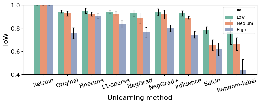
(a) Entanglement Score (ES) vs ToW

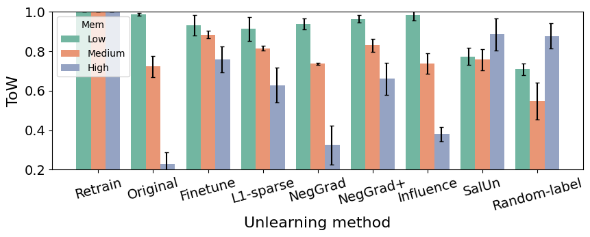
(b) Memorization vs ToW

Figure 1: Uncovering two factors that affect unlearning difficulty according to ToW (where higher is better). Left: the more entangled the retain and forget sets are in the embedding space, the harder it is to unlearn. Right: the less memorized a forget set is (thus having influenced the model less), the easier it is to unlearn (for most algorithms). Error bars correspond to 95% confidence intervals from running each algorithm 3 times (6 times for relabelling-based that had higher variance).

Our investigation hinges on generating three different forget/retain partitions with different degrees of entanglement: low, medium, and high. But, Equation (2) does not directly suggest a procedure for generating retain/forget partitions with a desired ES score. Hence, we achieved this indirectly using a proxy. Specifically, let $d(i,\mu;\theta^{o})=||\phi_{i}-\mu||^{2}$ denote the l2-distance in the original model’s embedding space between example $i$ and centroid $\mu$, as defined above. We compute this distance for each example in $\mathcal{D}_{train}$ and sort those examples according to their $d$-values. We then form each forget set to contain a contiguous subset of examples from different ranges of that sorted list. We find that this procedure allows us to construct retain/forget partitions of varying ES values. The ES values for our low, medium and high partitions are 309.94$\pm$98.56, 1076.99$\pm$78.64, 1612.21$\pm$110.82 for CIFAR-10, and 963.82$\pm$113.53, 2831.24$\pm$558.63, and 3876.90$\pm$426.92 for CIFAR-100. We include details of this procedure in the Section A.3, and visualizations to confirm the degree of retain/forget entanglement is in line with the scores we compute. We experiment on two datasets and two architectures, CIFAR-10/CIFAR-100 and ResNet-18/ResNet-50 with $|S|=3000$. Refer to Section A.2 for implementation details and Section A.6 for more detailed results for both datasets.

We observe from Figure 1(a) that it is harder to unlearn when the retain and forget sets are more entangled: all unlearning algorithms have poorer performance for highly-entangled vs lower-entangled settings. Further, we notice that different unlearning algorithms suffer disproportionately as the entanglement increases. Notably, methods based on relabelling (SalUn and Random-label) perform very poorly when the entanglement is high. We hypothesize that this is because, if two examples $i$ and $j$ are close neighbours in embedding space, with $i$ in the forget set and $j$ in the retain set, forcing example $i$ to be confidently predicted as an incorrect class (as relabelling algorithms do) will also cause $j$ to be predicted as that incorrect class, too, thus causing a drop in retain accuracy, which is captured by ToW. This effect will be less pronounced if $i$ and $j$ are far from each other.

4.2 The more memorized the forget examples are, the harder unlearning becomes

Feldman et al Feldman (2020) have already established that models must memorize some atypical examples in order to perform well. Further, prior literature has also established that noisy examples (that are more likely to be memorized) witness more “forgetting events” during training (their predicted label flips to an incorrect one) Toneva et al. (2018) and that models trained with Differential Privacy (DP), a procedure where noise is added to the gradients (making it harder to memorize), find it primarily hard to correctly predict atypical examples Carlini et al. (2019). In this section, we build upon these prior insights by investigating the connection between the degree of memorization of the forget set and difficulty of unlearning.

Let’s begin by inspecting Definition 2.2: if an example is not really memorized, the predictions of the model on that example will not change much whether the example was included in training or not. This implies that even the original model (no unlearning) is similar to retrain-from-scratch in terms of predictions on those examples, making unlearning unnecessary or trivial. On the other hand, for highly-memorized examples, the predictions between the original and retrained models will differ significantly, implying that an unlearning algorithm has “more work” to do to turn the original model into one that resembles the retrained one. We now investigate how the level of memorization of the forget set affects the behaviour of state-of-the-art unlearning algorithms. We hypothesize, based on our above intuition, that unlearning is easier when the forget set contains less-memorized examples.

To investigate this, we first compute the memorization score $\text{mem}(\mathcal{A},\mathcal{D}_{train},i)$ of each example $i\in\mathcal{D}_{train}$ and we sort all examples according to their scores. We then use that sorted list to create three different forget sets, corresponding to the lowest $N$ scores (“low-mem”), the highest $N$ (“high-mem”), and the $N$ that are nearest to 0.5, i.e. the midpoint of the range of memorization scores (“medium-mem”), where $N=3000$. We then apply different unlearning algorithms on each of these forget sets and compute ToW. We perform this experiment on CIFAR-10 using ResNet-18 and on CIFAR-100 using ResNet-50. Refer to Section A.2 for implementation details.

We first emphasize two key sets of conclusions. First, in terms of ToW, Figure 1(b) shows that, indeed, for most algorithms, the lower the memorization level of the forget set, the easier the problem is. In line with our prior discussion, even the original model performs well on “low-mem”, but performs very poorly on “high-mem”. Interestingly though, the two relabelling-based algorithms (SalUn and Random-label) follow an inverse trend: they perform better for higher-memorized forget sets. Second, breaking down ToW into its parts, we find interesting trends in terms of the forget set accuracy, in Figure 8. Specifically, for several unlearning algorithms, the forget accuracy for “low-mem” is still very high after unlearning them, as the model can infer the correct labels for such examples even when they weren’t included in training; this follows directly by Definition 2.2 if unlearning is done by retraining, and is shown here for the first time for approximate unlearning algorithms. On the other hand, we find that, for “high-mem”, different unlearning algorithms can (to varying degrees) cause the forget set accuracy to drop substantially; this is consistent with both Toneva et al. (2018) and Carlini et al. (2019), but shown here for the first time for approximate unlearning algorithms. Notably, we find that relabelling-based algorithms cause a larger drop in the accuracy of the forget set, relative to other approaches. This benefits ToW in the case of “high-mem” forget sets, where retraining has poor accuracy on this set (so they get rewarded by matching it), but it hurts on “low-mem”, since it causes a large discrepancy from retraining, which has high accuracy on this set (since it makes similar predictions to the original model on this set, by definition, and the original model has high accuracy on all of $\mathcal{D}_{train}$).

Overall, we have presented the first investigation into the behaviour of unlearning algorithms applied on forget sets of different degrees of memorization. A key finding is that different algorithms outshine others for different forget sets. Most notable is the failure of relabelling-based algorithms on the “low-mem” forget set, which is easy for other algorithms and, in fact, even no unlearning in that case might be an acceptable solution. We intuit that this is due to their aggressive unlearning strategy yielding “overforgetting” (producing a forget set accuracy that is lower than that of retraining from scratch) as discussed above. Furthermore, we observe that different unlearning algorithms work best for the “low-mem”, “medium-mem” and “high-mem” forget sets. Concretely, from Figure 1(b) we note that Finetune is best for “medium-mem”, SalUn is best for “high-mem”, and a number of algorithms are top-performers for “low-mem” (including no unlearning). This reveals a possible pathway for improving unlearning based on using different algorithms for different forget sets. So, how can one build on these insights to further improve unlearning algorithms performance?

5 Refined-Unlearning Meta-algorithm (RUM) for Improved Unlearning

Previously, we observed that unlearning algorithms have different behaviours on forget sets with different properties. For example, while “low mem” forget sets are almost trivial to unlearn (and even doing nothing may be acceptable), SalUn and Random-label perform poorly on them. On the other hand, SalUn and Random-label evidently outperform other unlearning algorithms on “high mem”. These observations suggest that the optimal unlearning algorithm to use is dependent on the properties of the forget set. One could therefore pick the best unlearning algorithm for each unlearning request, based on these factors. However, in practical scenarios, forget sets may be distributed differently than in our preliminary experiments, that were designed to cleanly separate different factors of interest. Indeed, real-world forget sets would likely contain a mixture of examples from different modes of the data distribution, some rare or highly-memorized while others common and not memorized at all. So, what can be done about these expected heterogeneous forget sets? How can our insights above be leveraged to improve unlearning for such cases?

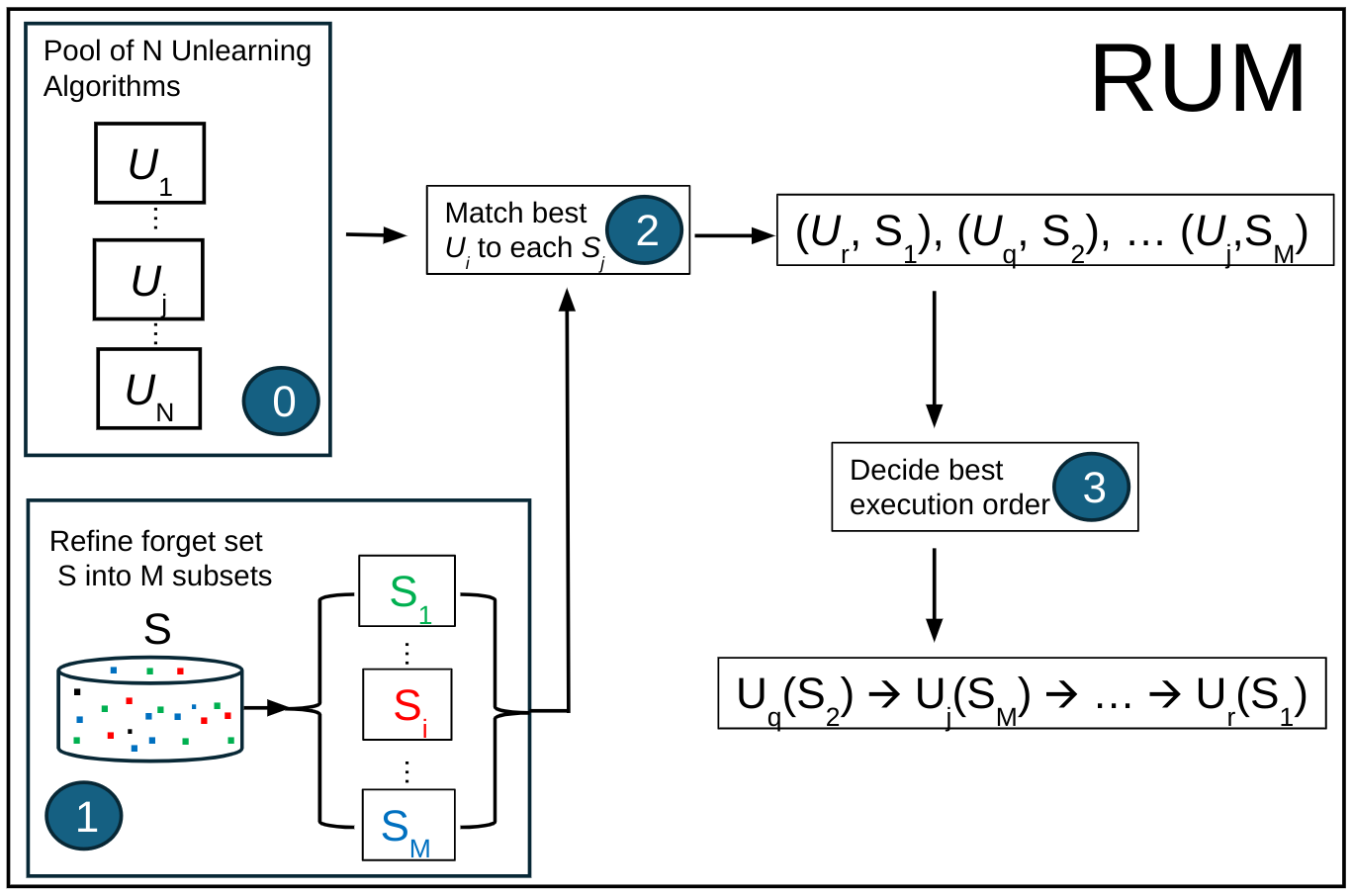
Figure 2: Overview of RUM.

To address this, we first propose a refinement procedure that divides forget sets into homogeneous subsets (with respect to the factors that we have found to affect the difficulty of unlearning and behaviours of existing algorithms). Second, we propose to utilize a pool of state-of-the-art algorithms to unlearn different subsets. Put together, we propose a Refined-Unlearning Meta-algorithm (RUM), comprised of two steps: 1) Refinement and 2) Meta-unlearning. Figure 2 overviews RUM.

Step 1: Refinement.

We introduce a function $\mathcal{F}$ that partitions the forget set $S$ into $K$ subsets: $\{S_{i}\}_{i=1}^{K}=\mathcal{F}(\mathcal{S})$ such that each forget set example appears in exactly one such subset. The intention of $\mathcal{F}$ is to generate homogeneous subsets w.r.t factor(s) that affect difficulty / algorithm’s behaviours.

Step 2: Meta-Unlearning.

Having obtained the subsets $\{S_{i}\}_{i=1}^{K}$ of $\mathcal{S}$, we now require a “meta-algorithm” $\mathcal{M}$ that dictates how to perform the individual unlearning requests and how to compose the resulting unlearned models to arrive to a model that has unlearned all of $\mathcal{S}$. In this work, we focus on meta-algorithms that tackle unlearning of subsets in a sequence, leaving other designs for future work. It therefore remains for our “meta-algorithm” to decide: i) what unlearning algorithm to apply for each subset, ii) what order should the unlearning requests be executed in.

More concretely, we assume access to a pool of existing unlearning algorithms $\mathcal{U}_{1}\dots\mathcal{U}_{N}$, like the ones described in related work, for instance. Let $\mathcal{M^{U}}(S_{i})$ denote a procedure that takes as input a subset $S_{i}$ and returns an unlearning algorithm $\mathcal{U}\in\{\mathcal{U}_{1}\dots\mathcal{U}_{N}\}$ that will be used for that subset. This selection can be done by leveraging insights such as those in Section 4. Further, let $\mathcal{M^{O}}$ denote a procedure that takes as input the $K$ subsets of $\mathcal{S}$ and returns a sorted list $S^{\prime}=\mathcal{M^{O}}(\mathcal{F}(\mathcal{S}))$ containing the K subsets in the desired order of execution.

Given the above ingredients, RUM proceeds by executing $K$ unlearning requests in a sequence, with step $i$ of that sequence corresponding to unlearning subset $S^{\prime}[i]$ by applying $\mathcal{U}_{i}(\theta^{o},S^{\prime}[i],\mathcal{R}_{i})=\theta^{u}_{i}$, where $\theta^{u}_{i}$ denotes the unlearned model up to step $i$ and $\mathcal{U}_{i}=\mathcal{M^{U}}(S^{\prime}[i])$ and $\mathcal{R}_{i}=\mathcal{R}\cup\{S^{\prime}[i+1],\dots S^{\prime}[K]\}$ is the retain set for step $i$, containing $\mathcal{R}$ as well as all other subsets of $\mathcal{S}$ that have not yet been unlearned in the sequence so far. We finally return the unlearned model of the last step $\theta^{u}_{K}$.

Our RUM framework is meant as an analysis framework, surfacing new problems to be solved and offering new pathways into future state-of-the-art algorithms. Nonetheless, we contribute below specific top-performing RUM instantiations, with specific choices for $\mathcal{F}$ and for $\mathcal{M}$.

6 Experimenting with RUM flavours

We now present RUM instantiations using a refinement strategy based on memorization scores and experimental evaluations answering the following questions: Q1: How useful is refinement alone? That is, for a given unlearning algorithm $\mathcal{U}$, does applying $\mathcal{U}$ sequentially on the $K$ homogeneous subsets of $\mathcal{S}$ outperform applying $\mathcal{U}$ once on all of $\mathcal{S}$? Q2: Can we obtain further gains by additionally selecting the best-performing unlearning algorithm for each forget set subset? Q3: Are there interpetable factors behind the boost obtained by sequential unlearning of homogeneous subsets?

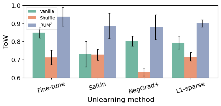
(a) CIFAR-10 with ResNet-18

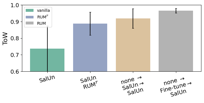
(b) CIFAR-10 with ResNet-18

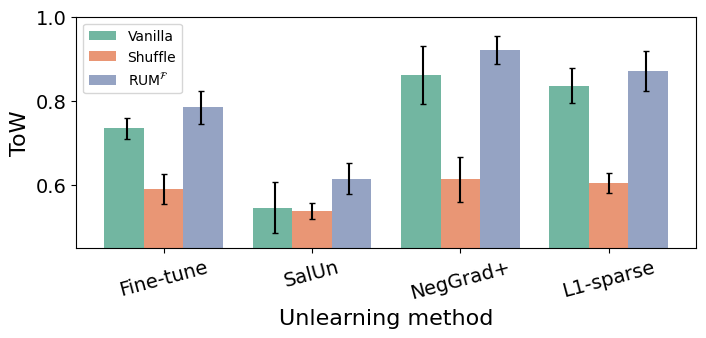
(c) CIFAR-100 with ResNet-50

Figure 3: From subplots a and c, we observe that RUM^F improves each unlearning algorithm. Vanilla corresponds to unlearning $\mathcal{S}$ in one go, whereas Shuffle and RUM^F operate sequentially on 3 subsets of $\mathcal{S}$. In the case of RUM^F, the 3 subsets are the result of applying $\mathcal{F}$ and the order is low $\rightarrow$ medium $\rightarrow$ high, whereas Shuffle uses equal-sized random subsets, serving as a control experiment. Further, from subplot b, we observe that full RUM, equipped with the best algorithm for each subset (do nothing $\rightarrow$ Fine-tune $\rightarrow$ SalUn), yields the overall best results (note: in CIFAR-100, NegGrad+ is the best algorithm, so full RUM corresponds to the RUM^F variant of NegGrad+).

	CIFAR-10		CIFAR-100
	ToW ($\uparrow$)	MIA gap ($\downarrow$)	ToW ($\uparrow$)	MIA gap ($\downarrow$)
Retrain	1.000$\pm$0.000	0.000	1.000$\pm$0.000	0.000
Fine-tune vanilla	0.849$\pm$0.030	0.120	0.734$\pm$0.025	0.139
Fine-tune shuffle	0.712$\pm$0.040	0.098	0.589$\pm$0.036	0.345
Fine-tune RUMF	0.937$\pm$0.052	0.099	0.784$\pm$0.040	0.093
L1-sparse vanilla	0.794$\pm$0.035	0.175	0.824$\pm$0.011	0.089
L1-sparse shuffle	0.716$\pm$0.023	0.257	0.604$\pm$0.023	0.353
L1-sparse RUMF	0.900$\pm$0.020	0.072	0.883$\pm$0.046	0.033
NegGrad+ vanilla	0.802$\pm$0.028	0.230	0.861$\pm$0.069	0.159
NegGrad+ shuffle	0.632$\pm$0.022	0.520	0.613$\pm$0.054	0.417
NegGrad+ RUMF	0.879$\pm$0.068	0.134	0.921$\pm$0.034	0.059
SalUn vanilla	0.731$\pm$0.070	0.374	0.545$\pm$0.061	0.372
SalUn shuffle	0.727$\pm$0.030	0.234	0.538$\pm$0.019	0.237
SalUn RUMF	0.887$\pm$0.069	0.031	0.614$\pm$0.037	0.181
RUM	0.965$\pm$0.014	0.034	0.921$\pm$0.034	0.059

Table 1: Each algorithm $\mathcal{U}$ is applied in three ways: i) in one-go (“vanilla”), ii) on a random partition of $\mathcal{S}$ into 3 equal-sized subsets, sequentially (“shuffle”), and iii) on three equal-sized subsets obtained by $\mathcal{F}$ in low $\rightarrow$ med $\rightarrow$ high order (“RUM^F”). In last row, RUM additionally chooses the best algorithm for each subset: none $\rightarrow$ Fine-tune $\rightarrow$ SalUn in CIFAR-10 and NegGrad+ RUM^F in CIFAR-100.

Experimental setup

We experiment with a refinement strategy based on memorization scores where $K$ = 3. Specifically, we study unlearning a forget set $\mathcal{S}$ that is the union of the three sets containing the $N$ lowest, the $N$ closest to 0.5, and the $N$ highest memorized examples in the dataset, where $N=1000$, making the overall size of the forget set 3000. We conduct experiments in two different datasets: CIFAR-10 and CIFAR-100, using ResNet-18 and ResNet-50, respectively. We evaluate unlearning algorithms both in terms of ToW, as before, and using a commonly-used MIA (Fan et al., 2023; Liu et al., 2024) that is a binary classifier trained to separate $\mathcal{R}$ from $\mathcal{D}_{test}$ and then queried on examples from $\mathcal{S}$. Following previous work, we report as “MIA” the fraction of examples from $\mathcal{S}$ that were predicted to be held-out. The goal is to match the “MIA” score of retrain-from-scratch. For convenience, we report the “MIA gap”: the absolute difference of the MIA score of unlearning from the MIA score of retrain-from-scratch (lower is better). See Section A.4 for details. We also consider and analyze the effect of two different orderings: i) low $\rightarrow$ medium $\rightarrow$ high and i) high $\rightarrow$ medium $\rightarrow$ low.

How useful is refinement alone?

To investigate this, we selected a subset of highest-performing algorithms and apply each algorithm $\mathcal{U}$ in three ways: i) “vanilla”, i.e. applying $\mathcal{U}(\theta^{o},\mathcal{S},\mathcal{R})$ as usual, ii) “shuffle” where $\mathcal{U}$ is applied sequentially on three equal-sized subsets of $\mathcal{S}$ that were determined randomly, and iii) RUM^F, where $\mathcal{U}$ is applied sequentially on the subsets obtained by $\mathcal{F}(\mathcal{S})$, i.e. utilizing only the refinement step of RUM and applying the same $\mathcal{U}$ on each subset. We include “shuffle” as a control experiment, so that any gain of RUM^F over shuffle is due to homogenization rather than simply reducing the size of the forget set or other effects of sequential unlearning. We observe from Figure 3 and Tables 11(a) and 11(b) that, for four different unlearning algorithms and on two different datasets, RUM^F significantly outperforms “vanilla” and “shuffle”, indicating that operating sequentially on homogenized subsets according to memorization can boost the performance of unlearning algorithms. Interestingly, in most cases, “shuffle” actually performs worse than “vanilla”, indicating that the difficulty of the problem may increase rather than decrease given a poor refinement strategy.

Can we further boost performance by per-subset algorithm selection?

To answer this, we leverage our findings from Section 4 to identify the best unlearning algorithm for each of the “low-mem”, “medium-mem” and “high-mem” scenarios. On CIFAR-10, this corresponds to doing nothing for low-mem (i.e. using the original model directly), using Fine-tune for medium-mem and SalUn for high-mem (based on Figure 1(b)). From Figure 3(b) (and Table 11(a)), we observe that we get the overall best results by far, both in terms of ToW and MIA, by applying RUM with “nothing $\rightarrow$ Fine-tune $\rightarrow$ SalUn”, demonstrating the value of incorporating our insights into unlearning pipelines. In fact, lets revisit our previous observation that SalUn and Random-Label perform uncharacteristically poorly on the “low-mem” forget set. In line with our hypothesis, we notice that “nothing $\rightarrow$ SalUn $\rightarrow$ SalUn” outperforms applying SalUn on all three subsets (a.k.a. SalUn RUM^F). Note that, for CIFAR-100, the best algorithm for all subsets is NegGrad+, so full RUM corresponds to NegGrad+ RUM^F.

Analysis of sequence dynamics

We report ToW and MIA with different orderings in Tables 11(a) and 11(b). We find that, while ToW is similar for different orderings, MIA can vary. To better understand these dynamics, we inspect the accuracies on $\mathcal{S}$ and its subsets after each step in Figure 4 for SalUn^F on CIFAR-10 and in Figure 9 for NegGrad+^F CIFAR-100. The former reveals why SalUn^F with low $\rightarrow$ med $\rightarrow$ high order greatly outperforms vanilla SalUn. Recall that we identified in Section 4.2 that SalUn “overforgets” low-mem examples (its forget accuracy is lower than that of retraining). We observe from Figure 4 that future steps of the sequence neutralize that overforgetting effect on low-mem, leading to better ToW (see Figure 3). Interestingly, in line with our previous insights (Section 4.2), we find (from both Figures 4 and 9) that it is hard to cause the “low-mem” accuracy to become low and stay low. NegGrad+ does not drop it for any order of execution; SalUn drops it in the first ordering, but that drop is later reversed. We leave it to future work to further study these sequential dynamics and their helpful or harmful effects on Tow and MIA. The fact that MIA results differ based on the sequence may tie in with the recently-identified “privacy onion effect” Carlini et al. (2022b).

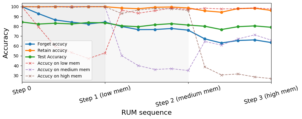
(a) low $\rightarrow$ med $\rightarrow$ high (MIA gap: 0.031)

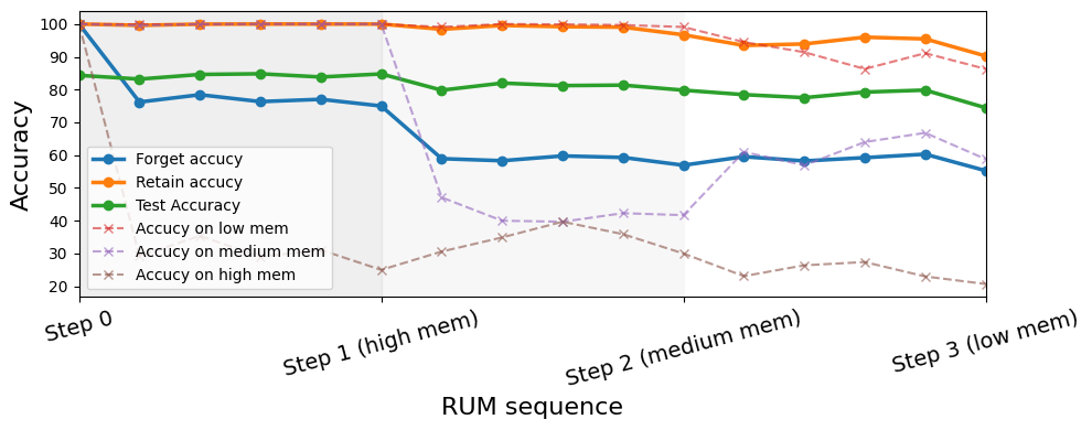
(b) high $\rightarrow$ med $\rightarrow$ low (MIA gap: 0.221)

Figure 4: Sequence dynamics for SalUn RUM^F on CIFAR-10. We report the accuracy on overall $\mathcal{S}$, $\mathcal{R}$ and $\mathcal{D}_{test}$, and subsets of $\mathcal{S}$ after each step. Both orderings yield similar Tow (see Table 11(a)).

7 Discussion and conclusion

We presented the first investigation into interpretable factors that affect the difficulty of unlearning. We found that unlearning gets harder i) the more entangled the forget and retain sets are in embedding space and ii) the more memorized the forget set is. Our investigation led into uncovering previously-unknown behaviours of state-of-the-art algorithms that were not surfaced when considering random forget sets: when do they fail, when do they excel and when do they exhibit different trends from each other. Notably, we discovered that relabelling-based methods suffer disproportionately as the embedding-space entanglement increases, and exhibit a reverse trend compared to other methods in their behaviour for different memorization levels. Armed with these insights, we then proposed the RUM framework surfacing new (sub)problems within unlearning, whose solution may lead to greater performance. Finally, we derived specific instantiations of RUM and analyzed how its different components can improve performance. We found that sequential unlearning of homogenized forget set subsets improves all considered state-of-the-art unlearning algorithms and investigated the dynamics of sequential unlearning to glean insights as to why that is. We also found that we can further boost performance by selecting the best unlearning algorithm per subset.

Efficiency

How is this important aspect affected in our sequential framework? We remark that it depends on the unlearning algorithm. For instance, applying Fine-tune three times is much more expensive than applying it once, because Fine-tune performs (at least) one epoch over the entire retain set. But for other algorithms the overall cost does not increase significantly. Further, a key observation from our results is that we can do well by actually doing nothing on a subset of the forget set, which can really boost efficiency (especially since the vast majority of examples are “low mem”).

Data-space vs embedding-space outliers

How does the embedding space entanglement interact with the level of memorization of the forget set? We analyzed this and found in Table 3 that all of our memorization buckets have relatively high ES, indicating that separating out (data-space) outliers in the forget set doesn’t lead to lower entanglement between the two sets in the embedding space. We leave it to future work to study the interaction of these factors.

Limitations and future work

We hope future work explores other refinement strategies (e.g. for a notion that captures embedding-space entanglement), designing refinement and meta-unlearning strategies that are practical, e.g. leveraging cheap proxies for quantities like memorization scores, investigating privacy implications of sequential RUM, e.g. in terms of the “privacy onion effect” Carlini et al. (2022b). We also hope to see how our RUM framework can be adopted and adapted for unlearning in LLMs, especially given the findings from the contemporaneous paper Barbulescu and Triantafillou (2024) where unlearning is performed only on the highest-memorized examples in the forget set (albeit, memorization is defined differently for LLMs). We hope our framework continues to enable progress in understanding and improving unlearning and that our identified factors of difficulty and associated behaviours of existing algorithms continue to improve the state-of-the-art and inform the development of strong evaluation metrics that consider forget sets that vary in terms of relevant identified characteristics.

8 Acknowledgements

We thank Vincent Dumoulin and Fabian Pedregosa for valuable conversations and feedback at various stages of the project.

Appendix A Appendix / supplemental material

A.1 Broader impact

Unlearning research can have profound broader impact in allowing users to request their data to be deleted from models or making models safer or more accurate by removing harmful or outdated information. Our work is exploratory: we identify factors affecting difficulty that are interpretable and can drive improvements to unlearning pipelines. As such, we don’t see any direct harmful impact of our work.

A.2 Implementation details

Datasets and models

We use CIFAR-10 and CIFAR-100 datasets for our evaluation. The CIFAR-10 dataset consists of 60,000 32x32 color images, including 10 classes of 6000 images each. The CIFAR-100 dataset has 100 classes, each containing 600 32x32 color images. In our experiments, the sizes of train, validation, and test sets are 45000, 5000, and 10000 respectively. We use ResNet-18 and ResNet-50 as model architectures. Specifically, ResNet-18 is used for CIFAR-10 and ResNet-50 is used for CIFAR-100, respectively.

Training details for original models

We trained a ResNet-18 model on the CIFAR-10 dataset and a ResNet-50 model on the CIFAR-100 dataset. For CIFAR-10, the ResNet-18 model was trained for 30 epochs using the SGD optimizer. The learning rate was initialized at 0.1 and scheduled with a cosine decay. We used a weight decay of 0.0005, a momentum of 0.9, and a batch size of 256. For CIFAR-100, the ResNet-50 model was trained for 150 epochs using the SGD optimizer. The learning rate was initialized at 0.1 and decayed by a factor of 0.2 at 60 and 120 epochs. We applied a weight decay of 0.0005, a momentum of 0.9, and a batch size of 256. Additionally, data augmentations, including random cropping and random horizontal flipping, were employed during training on CIFAR-100. All models were trained on Nvidia RTX A5000 GPUs.

Training details for machine unlearning

To ensure optimal performance, we carefully set the hyperparameters for each unlearning method across different datasets and architectures. For retrain-from-scratch, we followed the exact same training procedure as the original model, but only trained on the retain set, excluding the forget set. For Fine-tune, we trained the model for 10 epochs with a learning rate in the range [0.01, 0.1]. L1-sparse was run for 10 epochs with a learning rate in the range [0.005, 0.1] and a sparsity-promoting regularization parameter $\gamma$ in the range [$10^{-6}$, $10^{-4}$]. NegGrad was also trained for 10 epochs, with a learning rate in the range [$10^{-4}$, 0.1]. For NegGrad+, we used a $\beta$ value in the range [0.85, 0.99] as a weighting factor that balances two components of the loss, training for 5 epochs with a learning rate in the range [0.01, 0.05]. Influence unlearning involved tuning the parameter $\alpha$ for the woodfisher Hessian Inverse approximation within the range [1, 100]. SalUn was trained for 5-10 epochs with a learning rate in the range [0.005, 0.1] and sparsity ratios in the range [0.3, 0.7]. Random-label was trained for 10 epochs with a learning rate in the range [0.01, 0.1].

In our experiments with forget / retain set partitions at varied levels of memorization or ES, we tuned the hyperparameters to achieve the best ToW performance for each unlearning algorithm. The results are reported as averages with 95% confidence intervals over 3 runs, except for relabeling-based methods, which had higher variance and were therefore run 6 times. For the RUM experiment, we adjusted the hyperparameters at each step to ensure that the accuracy after each step closely matched the accuracy obtained by retraining from scratch. This procedure was repeated for all algorithms, with results reported as averages over 3 runs with 95% confidence intervals.

A.3 Procedure for creating retain / forget partitions with varying ES

To create retain / forget partitions with varied levels of ES, we followed a systematic procedure. Initially, we trained the original model $\theta^{o}$ on the entire training dataset $\mathcal{D}_{train}$. Using $\theta^{o}$, we then extracted embeddings for each data point in $\mathcal{D}_{train}$. The global centroid for $\mathcal{D}_{train}$, denoted as $\mu$, was determined by calculating the mean of all example embeddings. For each example $i$ in $\mathcal{D}_{train}$, we then computed its $l2$-distance from the global centroid $\mu$ in the original model’s embedding space as follows:

$$d(i,\mu;\theta^{o})=||\phi_{i}-\mu||^{2}$$ (3)

We ranked these distances for all data examples in $\mathcal{D}_{train}$ and selected the 3000 examples with the highest distances to form the low ES bucket. Subsequently, we moved further down the ranked list, selecting 3000 examples with progressively lower distances to form the medium and high ES buckets, until we achieved the desired levels of ES variation. This approach allowed us to form forget sets, each with a size of 3000, categorized into low, medium, and high ES levels. The rationale behind this selection is that examples with high distances from the global centroid are considered “distant" from the overall data distribution in the embedding space and are therefore less entangled with the rest of the dataset, i.e., the retain set. Various unlearning algorithms were then deployed on $\theta^{o}$ across different forget / retain partitions. Their performance was measured using ToW along with forget, retain, and test accuracy, as well as MIA.

This procedure enabled us to create retain / forget partitions with varying ES values. The ES values for our low, medium, and high ES partitions are shown in Table 2. As observed from the table, the ES values increase from low to high ES partitions for both CIFAR-10 and CIFAR-100, confirming the effectiveness of our procedure.

Additionally, Figure 5 presents the data representation of low, medium, and high ES partitions, confirming that the degree of entanglement between the retain and forget sets aligns with the computed ES values. As we move from low to high ES partitions, the forget set (yellow) and the retain set (blue) become increasingly entangled. This indicates that higher ES partitions reflect greater complexity in distinguishing between the two sets.

	Low ES	Medium ES	High ES
ES value	309.94$\pm$98.56	1076.99$\pm$78.64	1612.210$\pm$110.82

(a) CIFAR-10

	Low ES	Medium ES	High ES
ES value	963.82$\pm$113.53	2831.24$\pm$558.63	3876.90$\pm$426.92

(b) CIFAR-100

Table 2: ES values for the low, medium and high forget / retain partitions for CIFAR-10 and CIFAR-100.

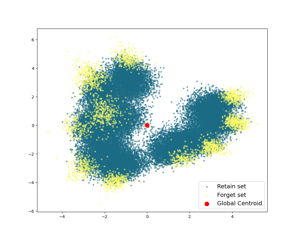
(a) low ES

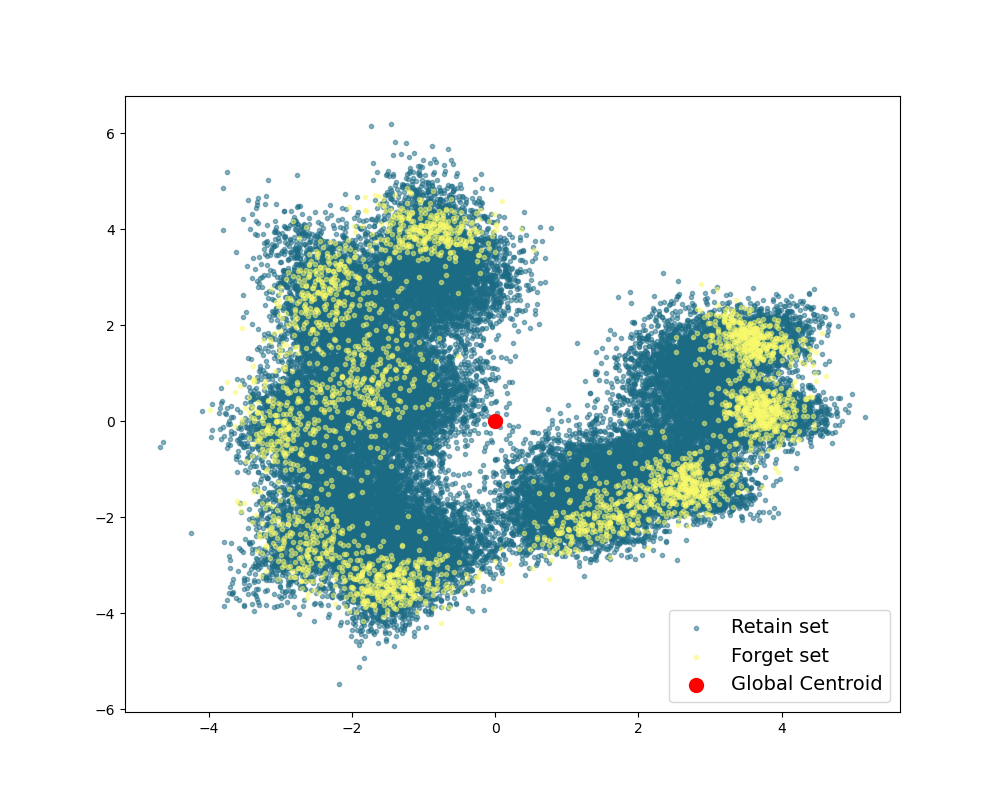
(b) medium ES

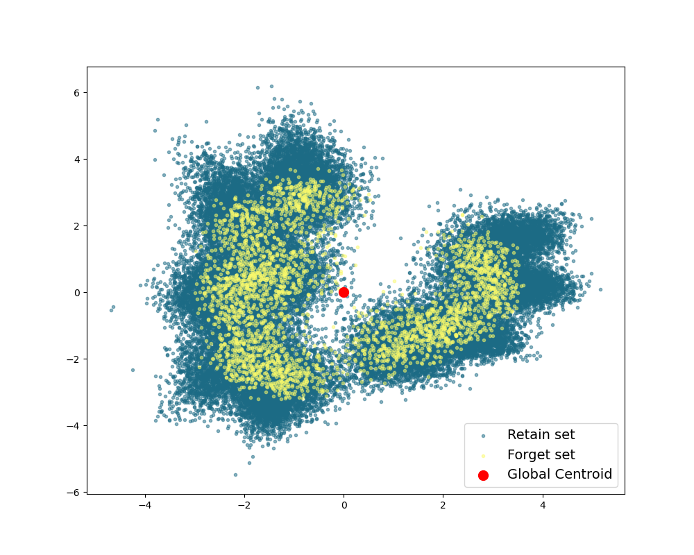
(c) high ES

Figure 5: Data representation visualization for forget / retain partitions with low, medium, and high ES. We used PCA to reduce the dimensionality for visualization. In each figure, the data examples from the forget set are shown in yellow, while those from the retain set are in blue. The global centroid is marked in red at the center of the figures.

A.4 Description of MIA

We adopted a MIA based on prediction confidence, following the procedure described by Liu et al. [2024]. To conduct this attack, we first sampled equal-sized data from the retain set and the test set, using these to train a binary classifier as the MIA model. This model is designed to distinguish whether a data example was involved in the training stage or not.

Next, we applied this attack model to the forget set to evaluate unlearning performance during the testing phase, after an unlearning method was implemented. Intuitively, for successful unlearning, we want forget set examples to be classified as “non-training” data. We define “training" data as the positive class and “non-training" data as the negative class, and measured the performance of MIA by calculating the ratio of true negatives (i.e., the number of the forgetting samples predicted as non-training examples) predicted by the MIA model to the total size of the forget set, as shown in (4), following the same procedure as prior work Liu et al. [2024].

$$\text{MIA Performance}=\frac{TN_{\mathcal{S}}}{|\mathcal{S}|},$$ (4)

In this context, $\mathcal{S}\subseteq\mathcal{D}_{train}$ represents the forget set and $|\mathcal{S}|$ is the total size of this set. The term $TN_{\mathcal{S}}$ denotes the number of true negatives predicted by the MIA model, indicating examples identified as “non-training” data. This metric ranges from 0 to 1, with higher values signifying a larger portion of the forget set predicted as “non-training” data. The ideal MIA score, for an unlearing algorithm, is one that matches the MIA score of retraining-from-scratch. Note that, even if applying this MIA on retrain-from-scratch, some portion of the forget set will be classified as “training data” due to heavily resembling the retain set (e.g. examples that are not really memorized may have similar confidences regardless on whether or not they were trained on). And we want the model confidences of the unlearned model to resemble as closely as possible those of retrain-from-scratch. For this reason, we additionally report the “MIA gap” (the absolute differentce between the MIA score for unlearning compared to that of retrain-from-scratch) as a easier-to-interpret metric, where lower is better, and the ideal score there is 0.

A.5 Data-space vs embedding-space outliers

Building on our discussion in Section 4, we identify two factors that affect the difficulty of unlearning: the entanglement between the forget and retain sets, and the memorization level of the forget examples. This raises the question: how do these two factors interact with each other? Are the outliers in data space the same as those in embedding space? Our findings in this section suggest that these factors are indeed distinct.

Memorization within ES-Based Partitions

We analyzed the memorization scores within each forget set categorized by different ES values. Figure 6 shows the distribution and average memorization scores in the forget sets of low, medium, and high ES categories. It can be seen that each ES category’s forget set contains a mix of memorization levels. Specifically, while the mean memorization score of forget examples increases from low to high ES categories, the memorization scores still span the entire range from 0 to 1.

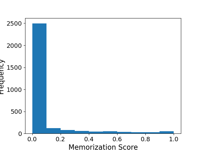
(a) low ES

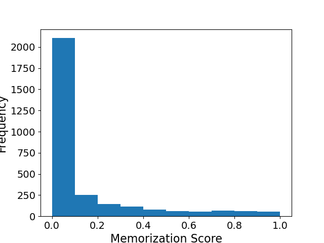
(b) medium ES

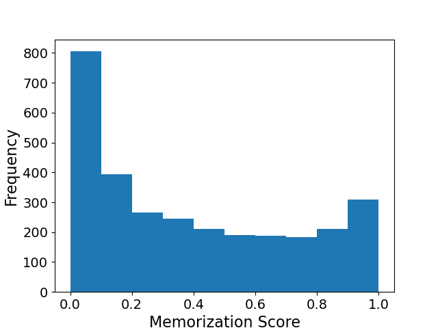
(c) high ES

CIFAR-10 with ResNet-18

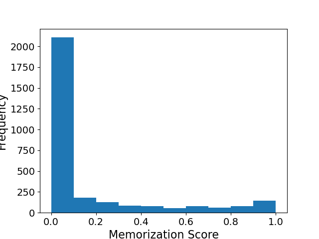
(d) low ES

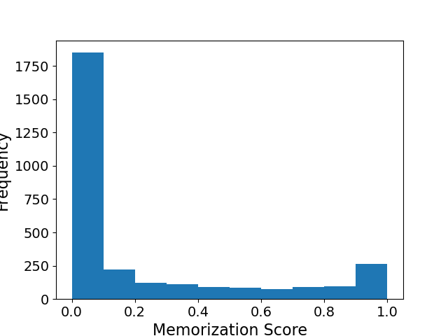
(e) medium ES

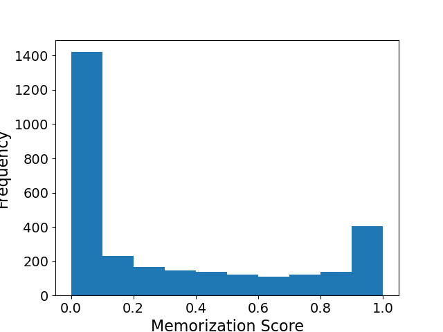
(f) high ES

CIFAR-100 with ResNet-50

Figure 6: Memorization distribution for low, medium, high ES forget / retain partitions. The mean memorization score for low, medium, high ES partitions are 0.084$\pm$0.203, 0.134$\pm$0.235, 0.390$\pm$0.326 for CIFAR-10, and 0.159$\pm$0.283, 0.222$\pm$0.329, and 0.317$\pm$0.364 for CIFAR-100.

Entanglement within Memorization-Based Partitions

We examined the ES values for each memorization category to understand the entanglement between the forget and retain sets in the embedding space. Table 3 presents the ES values corresponding to low, medium, and high memorization buckets. The findings reveal that all the memorization bucket exhibits relatively high ES, suggesting that separating outliers in the data space does not reduce the entanglement between the forget and retain sets in the embedding space.

	Low memorization	Medium memorization	High memorization
ES value	21134.127	32785.711	14736.591

(a) CIFAR-10

	Low memorization	Medium memorization	High mamorization
ES value	30028.924	58683.180	20528.561

(b) CIFAR-100

Table 3: ES values for forget / retain partitions across varied memorization levels for CIFAR-10 and CIFAR-100.

These findings demonstrate that embedding space entanglement and the memorization level of the forget set are distinct concepts, not merely different aspects of the same phenomenon.

A.6 Detailed results

In this section, we show the results that were used to construct all figures in the paper, as well as additional results and analyses.

Entanglement of forget and retain sets affects unlearning difficulty

The first factor affecting unlearning difficulty, as discussed in Section 4.1, is the degree of entanglement between the forget and retain sets in the embedding space. Specifically, the more entangled these sets are, the harder it becomes to unlearn. We present detailed results on how this factor affects unlearning difficulty in Table 4, 5, 6, and Figure 7. Table 4 displays the ToW results for different ES partitions for both CIFAR-10 and CIFAR-100. Comprehensive data, including forget, retain, test accuracy, and MIA performance, are provided in Figure 7, as well as in Table 5 for CIFAR-10 and Table 6 for CIFAR-100. All the results are averaged over 3 runs for each algorithm (6 runs for relabelling-based algorithms due to their higher variance), along with 95% confidence intervals.

	Low ES	Medium ES	High ES
Retrain	1.000 $\pm$ 0.000	1.000 $\pm$ 0.000	1.000 $\pm$ 0.000
Original	0.944 $\pm$ 0.014	0.928 $\pm$ 0.022	0.759 $\pm$ 0.048
Fine-tune	0.952 $\pm$ 0.024	0.923 $\pm$ 0.019	0.908 $\pm$ 0.018
L1-sparse	0.945 $\pm$ 0.013	0.926 $\pm$ 0.019	0.836 $\pm$ 0.031
NegGrad	0.929 $\pm$ 0.030	0.887 $\pm$ 0.047	0.766 $\pm$ 0.042
NegGrad+	0.941 $\pm$ 0.029	0.920 $\pm$ 0.038	0.800 $\pm$ 0.029
Influence Unlearning	0.928 $\pm$ 0.023	0.890 $\pm$ 0.012	0.744 $\pm$ 0.029
SalUn	0.783 $\pm$ 0.031	0.656 $\pm$ 0.046	0.618 $\pm$ 0.056
Random-label	0.767 $\pm$ 0.107	0.663 $\pm$ 0.055	0.443 $\pm$ 0.087

(a) CIFAR-10 with ResNet-18.

	Low ES	Medium ES	High ES
Retrain	1.000 $\pm$ 0.000	1.000 $\pm$ 0.000	1.000 $\pm$ 0.000
Original	0.836 $\pm$ 0.043	0.768 $\pm$ 0.036	0.690 $\pm$ 0.061
Fine-tune	0.878 $\pm$ 0.014	0.852 $\pm$ 0.006	0.773 $\pm$ 0.029
L1-sparse	0.867 $\pm$ 0.039	0.803 $\pm$ 0.025	0.709 $\pm$ 0.057
NegGrad	0.755 $\pm$ 0.027	0.707 $\pm$ 0.039	0.666 $\pm$ 0.060
NegGrad+	0.922 $\pm$ 0.055	0.844 $\pm$ 0.014	0.766 $\pm$ 0.022
Influence Unlearning	0.806 $\pm$ 0.027	0.756 $\pm$ 0.041	0.668 $\pm$ 0.037
SalUn	0.835 $\pm$ 0.037	0.704 $\pm$ 0.028	0.678 $\pm$ 0.042
Random-label	0.675 $\pm$ 0.029	0.629 $\pm$ 0.031	0.585 $\pm$ 0.014

(b) CIFAR-100 with ResNet-50.

Table 4: ToW for different unlearning algorithms applied to forget / retain sets with varying ES, evaluated on CIFAR-10 using ResNet-18 and CIFAR-100 using ResNet-50. Across all algorithms, including the baseline without any unlearning performed (denoted as “Original"), we observe that ToW decreases from low to high ES partitions, indicating that unlearning becomes harder as the forget and retain sets become more entangled.

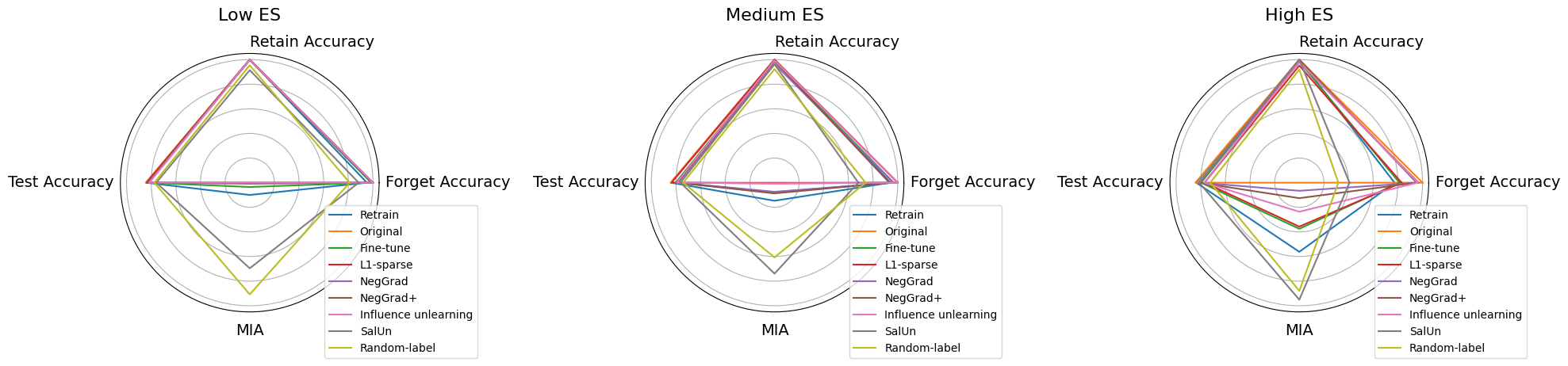
(a) CIFAR-10 with ResNet-18

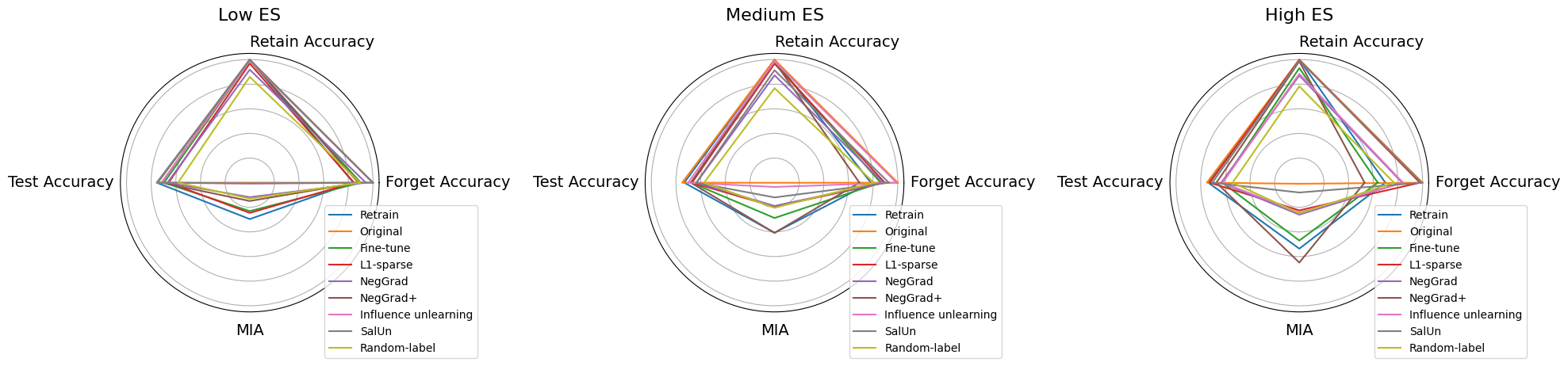
(b) CIFAR-100 with ResNet-50

Figure 7: Forget, retain, test accuracy and MIA performance for forget / retain partitions with varied ES, for CIFAR-10 using ResNet-18 and CIFAR-100 using ResNet-50. As the ES increases, there is a notable decline in forget accuracy and a significant rise in MIA performance. This trend indicates that as the forget and retain sets become more entangled, more information from the forget set is effectively removed after unlearning.

	Forget Acc	Retain Acc	Test Acc	MIA
Retrain	95.078 $\pm$ 0.995	100.000 $\pm$ 0.003	84.040 $\pm$ 1.387	0.100 $\pm$ 0.010
Original	100.000 $\pm$ 0.000	100.000 $\pm$ 0.000	84.353 $\pm$ 3.455	0.000 $\pm$ 0.000
Fine-tune	98.522 $\pm$ 3.296	99.675 $\pm$ 1.385	83.107 $\pm$ 3.862	0.035 $\pm$ 0.074
L1-sparse	100.000 $\pm$ 0.000	99.994 $\pm$ 0.022	83.787 $\pm$ 3.632	0.001 $\pm$ 0.001
NegGrad	99.800 $\pm$ 0.461	99.853 $\pm$ 0.429	81.740 $\pm$ 5.270	0.006 $\pm$ 0.007
NegGrad+	99.500 $\pm$ 0.647	99.988 $\pm$ 0.051	82.743 $\pm$ 6.193	0.007 $\pm$ 0.007
Influence unlearning	100.000 $\pm$ 0.000	99.964 $\pm$ 0.154	81.667 $\pm$ 2.547	0.000 $\pm$ 0.001
SalUn	88.400 $\pm$ 6.843	91.442 $\pm$ 2.438	75.833 $\pm$ 0.725	0.696 $\pm$ 0.172
Random-label	81.100 $\pm$ 10.427	95.396 $\pm$ 0.682	77.470 $\pm$ 4.529	0.908 $\pm$ 0.026

(a) Low ES

	Forget Acc	Retain Acc	Test Acc	MIA
Retrain	94.067 $\pm$ 0.722	100.000 $\pm$ 0.000	84.167 $\pm$ 1.243	0.147 $\pm$ 0.009
Original	100.000 $\pm$ 0.000	100.000 $\pm$ 0.000	84.353 $\pm$ 3.455	0.000 $\pm$ 0.000
Fine-tune	96.678 $\pm$ 3.525	98.655 $\pm$ 2.575	80.210 $\pm$ 3.004	0.078 $\pm$ 0.019
L1-sparse	99.978 $\pm$ 0.096	99.990 $\pm$ 0.044	83.580 $\pm$ 3.270	0.005 $\pm$ 0.014
NegGrad	96.300 $\pm$ 4.774	96.527 $\pm$ 4.294	78.163 $\pm$ 4.326	0.074 $\pm$ 0.057
NegGrad+	93.200 $\pm$ 4.241	98.907 $\pm$ 1.839	78.580 $\pm$ 4.404	0.087 $\pm$ 0.041
Influence unlearning	99.889 $\pm$ 0.172	99.372 $\pm$ 0.774	79.260 $\pm$ 0.774	0.007 $\pm$ 0.005
SalUn	68.044 $\pm$ 7.008	96.222 $\pm$ 6.649	76.380 $\pm$ 6.843	0.739 $\pm$ 0.270
Random-label	73.922 $\pm$ 3.527	92.244 $\pm$ 7.643	74.157 $\pm$ 10.427	0.607 $\pm$ 0.316

(b) Medium ES

	Forget Acc	Retain Acc	Test Acc	MIA
Retrain	77.300 $\pm$ 3.130	100.000 $\pm$ 0.003	83.653 $\pm$ 2.280	0.562 $\pm$ 0.026
Original	100.000 $\pm$ 0.000	100.000 $\pm$ 0.000	84.353 $\pm$ 3.455	0.000 $\pm$ 0.001
Fine-tune	81.289 $\pm$ 2.298	98.371 $\pm$ 1.395	79.763 $\pm$ 1.587	0.375 $\pm$ 0.066
L1-sparse	83.022 $\pm$ 14.615	95.164 $\pm$ 10.943	76.943 $\pm$ 6.159	0.357 $\pm$ 0.075
NegGrad	96.756 $\pm$ 3.705	97.925 $\pm$ 3.977	80.927 $\pm$ 6.576	0.066 $\pm$ 0.052
NegGrad+	95.222 $\pm$ 2.993	99.966 $\pm$ 0.065	81.447 $\pm$ 3.720	0.126 $\pm$ 0.055
Influence unlearning	96.111 $\pm$ 6.259	98.161 $\pm$ 3.205	77.093 $\pm$ 5.087	0.236 $\pm$ 0.044
SalUn	40.722 $\pm$ 11.043	99.967 $\pm$ 0.080	81.250 $\pm$ 3.335	0.951 $\pm$ 0.077
Random-label	31.656 $\pm$ 5.551	91.871 $\pm$ 0.275	72.273 $\pm$ 1.895	0.879 $\pm$ 0.055

(c) High ES

Table 5: Accuracy and MIA performance for different unlearning algorithms applied to forget / retain sets with varying ES for CIFAR-10 using ResNet-18.

	Forget Acc	Retain Acc	Test Acc	MIA
Retrain	84.222 $\pm$ 3.734	99.968 $\pm$ 0.012	75.493 $\pm$ 0.756	0.296 $\pm$ 0.041
Original	100.000 $\pm$ 0.000	99.959 $\pm$ 0.015	75.003 $\pm$ 2.809	0.000 $\pm$ 0.000
Fine-tune	90.044 $\pm$ 8.075	99.148 $\pm$ 1.639	69.577 $\pm$ 5.366	0.231 $\pm$ 0.067
L1-sparse	84.611 $\pm$ 6.139	96.807 $\pm$ 2.881	65.840 $\pm$ 3.228	0.246 $\pm$ 0.040
NegGrad	94.200 $\pm$ 2.319	91.843 $\pm$ 1.718	66.793 $\pm$ 3.820	0.118 $\pm$ 0.022
NegGrad+	88.111 $\pm$ 1.532	99.841 $\pm$ 0.162	71.493 $\pm$ 2.158	0.149 $\pm$ 0.028
Influence unlearning	99.722 $\pm$ 0.981	99.202 $\pm$ 2.531	71.610 $\pm$ 5.558	0.007 $\pm$ 0.020
SalUn	100.000 $\pm$ 0.000	99.952 $\pm$ 0.016	74.707 $\pm$ 2.064	0.006 $\pm$ 0.002
Random-label	89.267 $\pm$ 1.159	85.992 $\pm$ 0.557	58.190 $\pm$ 1.640	0.130 $\pm$ 0.023

(a) Low ES

	Forget Acc	Retain Acc	Test Acc	MIA
Retrain	78.133 $\pm$ 1.616	99.960 $\pm$ 0.009	73.273 $\pm$ 2.131	0.407 $\pm$ 0.007
Original	100.000 $\pm$ 0.000	99.959 $\pm$ 0.015	75.003 $\pm$ 2.809	0.001 $\pm$ 0.001
Fine-tune	86.078 $\pm$ 8.732	98.069 $\pm$ 4.782	67.680 $\pm$ 4.230	0.287 $\pm$ 0.040
L1-sparse	89.511 $\pm$ 4.761	96.656 $\pm$ 2.561	66.983 $\pm$ 3.893	0.195 $\pm$ 0.025
NegGrad	88.289 $\pm$ 1.800	87.242 $\pm$ 2.187	63.380 $\pm$ 3.313	0.189 $\pm$ 0.018
NegGrad+	68.900 $\pm$ 2.582	98.251 $\pm$ 1.412	67.913 $\pm$ 1.354	0.408 $\pm$ 0.035
Influence unlearning	98.978 $\pm$ 1.962	98.613 $\pm$ 2.268	70.093 $\pm$ 0.981	0.035 $\pm$ 0.042
SalUn	92.744 $\pm$ 1.706	91.400 $\pm$ 1.657	63.460 $\pm$ 1.319	0.120 $\pm$ 0.011
Random-label	80.622 $\pm$ 0.751	76.779 $\pm$ 0.664	57.213 $\pm$ 1.410	0.204 $\pm$ 0.004

(b) Medium ES

	Forget Acc	Retain Acc	Test Acc	MIA
Retrain	69.789 $\pm$ 6.038	99.963 $\pm$ 0.012	73.827 $\pm$ 3.116	0.536 $\pm$ 0.073
Original	99.989 $\pm$ 0.048	99.960 $\pm$ 0.018	75.003 $\pm$ 2.809	0.009 $\pm$ 0.007
Fine-tune	63.622 $\pm$ 6.326	93.054 $\pm$ 2.972	62.320 $\pm$ 3.726	0.470 $\pm$ 0.060
L1-sparse	97.856 $\pm$ 1.519	99.706 $\pm$ 0.286	72.620 $\pm$ 1.985	0.225 $\pm$ 0.057
NegGrad	83.489 $\pm$ 23.803	87.013 $\pm$ 19.000	63.343 $\pm$ 12.854	0.260 $\pm$ 0.245
NegGrad+	52.944 $\pm$ 5.967	98.491 $\pm$ 0.732	67.257 $\pm$ 2.996	0.649 $\pm$ 0.091
Influence unlearning	84.133 $\pm$ 8.032	88.398 $\pm$ 5.947	62.170 $\pm$ 1.267	0.242 $\pm$ 0.046
SalUn	99.167 $\pm$ 1.444	99.289 $\pm$ 1.222	70.567 $\pm$ 2.274	0.080 $\pm$ 0.058
Random-label	76.756 $\pm$ 4.633	78.256 $\pm$ 4.378	54.160 $\pm$ 1.832	0.250 $\pm$ 0.041

(c) High ES

Table 6: Accuracy and MIA performance of different unlearning algorithms on forget / retain sets with varying ES for CIFAR-100 using ResNet-50.

Memorization of forget examples affects unlearning difficulty

In Section 4.2, we discussed another critical factor affecting unlearning difficulty: the memorization level of the forget examples. Specifically, when a forget set consists of examples that are more highly memorized by the model, it becomes more difficult to unlearn (for most algorithms). The detailed results that support this observation are presented in Table 7, Table 8, Table 9, and Figure 8.

Table 7 illustrates the ToW for forget sets with varying memorization levels. Additionally, Figure 8 and the tables for CIFAR-10 (Table 8) and CIFAR-100 (Table 9) provide extensive data on forget, retain, and test accuracy, as well as MIA performance. For all the experiments, the average results are reported with 95% confidence intervals over 6 runs for relabelling-based algorithms and 3 runs for others.

	Low memorization	Medium memorization	High memorization
Retrain	1.000 $\pm$ 0.000	1.000 $\pm$ 0.000	1.000 $\pm$ 0.000
Original	0.988 $\pm$ 0.007	0.723 $\pm$ 0.053	0.231 $\pm$ 0.058
Fine-tune	0.933 $\pm$ 0.052	0.884 $\pm$ 0.019	0.760 $\pm$ 0.065
L1-sparse	0.914 $\pm$ 0.061	0.816 $\pm$ 0.011	0.629 $\pm$ 0.087
NegGrad	0.938 $\pm$ 0.028	0.738 $\pm$ 0.005	0.325 $\pm$ 0.098
NegGrad+	0.965 $\pm$ 0.020	0.831 $\pm$ 0.032	0.661 $\pm$ 0.082
Influence unlearning	0.986 $\pm$ 0.031	0.738 $\pm$ 0.051	0.381 $\pm$ 0.037
Salun	0.774 $\pm$ 0.043	0.758 $\pm$ 0.053	0.886 $\pm$ 0.082
Random-label	0.709 $\pm$ 0.029	0.548 $\pm$ 0.093	0.877 $\pm$ 0.064

(a) CIFAR-10 with ResNet-18

	Low memorization	Medium memorization	High memorization
Retrain	1.000 $\pm$ 0.000	1.000 $\pm$ 0.000	1.000 $\pm$ 0.000
Original	0.983 $\pm$ 0.014	0.516 $\pm$ 0.041	0.026 $\pm$ 0.005
Fine-tune	0.974 $\pm$ 0.064	0.830 $\pm$ 0.052	0.768 $\pm$ 0.025
L1-sparse	0.857 $\pm$ 0.035	0.828 $\pm$ 0.021	0.754 $\pm$ 0.036
NegGrad	0.680 $\pm$ 0.130	0.564 $\pm$ 0.044	0.270 $\pm$ 0.039
NegGrad+	0.986 $\pm$ 0.024	0.917 $\pm$ 0.040	0.889 $\pm$ 0.012
Influence unlearning	0.960 $\pm$ 0.112	0.556 $\pm$ 0.044	0.154 $\pm$ 0.081
SalUn	0.964 $\pm$ 0.091	0.564 $\pm$ 0.047	0.538 $\pm$ 0.061
Random-label	0.770 $\pm$ 0.105	0.548 $\pm$ 0.022	0.409 $\pm$ 0.044

(b) CIFAR-100 with ResNet-50

Table 7: ToW for different unlearning algorithms applied to forget sets with varying levels of memorization, for CIFAR-10 using ResNet-18 and CIFAR-100 using ResNet-50. As the memorization level of the forget examples increases, the ToW significantly decreases for most algorithms, indicating that unlearning becomes harder when the forget examples are more memorized by the model.

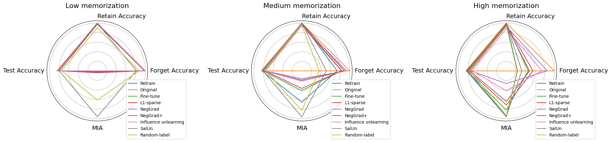
(a) CIFAR-10 with ResNet-18

(b) CIFAR-100 with ResNet-50

Figure 8: Forget, retain, test accuracy and MIA performance for forget / retain partitions with varying levels of memorization, for CIFAR-10 using ResNet-18 and CIFAR-100 using ResNet-50. As the memorization level of the forget sets increases, forget accuracy significantly decreases while MIA performance increases. This trend indicates that as the forget examples become more memorized by the model, unlearning becomes more effective in removing the effect of these examples.

	Forget accuracy	Retain accuracy	Test accuracy	MIA
Retrain	99.711 $\pm$ 0.253	100.000 $\pm$ 0.000	84.280 $\pm$ 1.184	0.010 $\pm$ 0.006
Original	100.000 $\pm$ 0.000	100.000 $\pm$ 0.000	84.353 $\pm$ 3.455	0.000 $\pm$ 0.000
Fine-tune	99.156 $\pm$ 1.634	98.390 $\pm$ 1.731	79.587 $\pm$ 3.173	0.020 $\pm$ 0.024
L1-sparse	98.678 $\pm$ 2.046	97.736 $\pm$ 0.449	78.750 $\pm$ 4.659	0.039 $\pm$ 0.047
NegGrad	99.178 $\pm$ 1.574	99.241 $\pm$ 1.512	79.390 $\pm$ 1.904	0.030 $\pm$ 0.033
NegGrad+	98.300 $\pm$ 1.490	99.944 $\pm$ 0.142	82.257 $\pm$ 3.363	0.020 $\pm$ 0.019
Influence unlearning	100.000 $\pm$ 0.000	100.000 $\pm$ 0.000	83.133 $\pm$ 4.128	0.002 $\pm$ 0.004
SalUn	81.278 $\pm$ 5.906	99.996 $\pm$ 0.003	79.223 $\pm$ 5.991	0.960 $\pm$ 0.053
Random-label	86.667 $\pm$ 6.902	90.604 $\pm$ 7.740	74.350 $\pm$ 1.287	0.611 $\pm$ 0.089

(a) Low memorization

	Forget accuracy	Retain accuracy	Test accuracy	MIA
Retrain	73.611 $\pm$ 3.478	100.000 $\pm$ 0.000	82.977 $\pm$ 2.060	0.654 $\pm$ 0.067
Original	100.000 $\pm$ 0.000	100.000 $\pm$ 0.000	84.353 $\pm$ 3.455	0.000 $\pm$ 0.000
Fine-tune	82.856 $\pm$ 1.706	99.422 $\pm$ 0.721	80.957 $\pm$ 2.376	0.413 $\pm$ 0.117
L1-sparse	82.922 $\pm$ 5.971	95.660 $\pm$ 5.166	77.130 $\pm$ 4.536	0.368 $\pm$ 0.013
NegGrad	92.900 $\pm$ 10.384	96.755 $\pm$ 6.091	77.593 $\pm$ 5.946	0.164 $\pm$ 0.130
NegGrad+	88.122 $\pm$ 5.826	99.962 $\pm$ 0.072	80.303 $\pm$ 5.202	0.193 $\pm$ 0.060
Influence unlearning	91.800 $\pm$ 13.743	96.267 $\pm$ 6.256	76.843 $\pm$ 5.060	0.217 $\pm$ 0.099
SalUn	51.100 $\pm$ 7.729	100.000 $\pm$ 0.000	80.847 $\pm$ 3.332	0.965 $\pm$ 0.012
Random-label	36.233 $\pm$ 6.904	94.675 $\pm$ 2.471	75.373 $\pm$ 2.546	0.829 $\pm$ 0.076

(b) Medium memorization

	Forget accuracy	Retain accuracy	Test accuracy	MIA
Retrain	23.444 $\pm$ 5.753	100.000 $\pm$ 0.000	82.967 $\pm$ 1.910	0.961 $\pm$ 0.018
Original	100.000 $\pm$ 0.000	100.000 $\pm$ 0.000	84.353 $\pm$ 3.455	0.002 $\pm$ 0.001
Fine-tune	45.822 $\pm$ 10.494	98.987 $\pm$ 4.112	82.003 $\pm$ 4.700	0.820 $\pm$ 0.135
L1-sparse	55.644 $\pm$ 16.226	97.001 $\pm$ 1.941	78.730 $\pm$ 5.902	0.714 $\pm$ 0.075
NegGrad	85.133 $\pm$ 15.675	93.289 $\pm$ 10.807	74.827 $\pm$ 7.390	0.266 $\pm$ 0.179
NegGrad+	48.400 $\pm$ 5.596	94.876 $\pm$ 2.829	75.783 $\pm$ 4.310	0.641 $\pm$ 0.107
Influence unlearning	74.567 $\pm$ 3.934	88.536 $\pm$ 2.176	71.143 $\pm$ 3.499	0.417 $\pm$ 0.067
SalUn	32.311 $\pm$ 5.235	99.560 $\pm$ 0.597	80.647 $\pm$ 3.328	0.951 $\pm$ 0.008
Random-label	22.700 $\pm$ 3.360	94.728 $\pm$ 4.453	76.323 $\pm$ 2.830	0.936 $\pm$ 0.025

(c) High memorization

Table 8: Accuracy and MIA results for various unlearning algorithms applied on forget / retain sets with different memorization levels for CIFAR10 using ResNet-18.

	Forget accuracy	Retain accuracy	Test accuracy	MIA
Retrain	99.878 $\pm$ 0.096	99.960 $\pm$ 0.003	74.077 $\pm$ 2.112	0.016 $\pm$ 0.005
Original	100.000 $\pm$ 0.000	99.959 $\pm$ 0.015	75.003 $\pm$ 2.809	0.001 $\pm$ 0.001
Fine-tune	99.878 $\pm$ 0.266	99.806 $\pm$ 0.273	71.693 $\pm$ 4.515	0.018 $\pm$ 0.015
L1-sparse	98.100 $\pm$ 0.299	95.385 $\pm$ 2.147	65.550 $\pm$ 2.179	0.040 $\pm$ 0.007
NegGrad	90.589 $\pm$ 2.987	85.454 $\pm$ 6.778	61.637 $\pm$ 6.310	0.140 $\pm$ 0.010
NegGrad+	99.556 $\pm$ 0.345	99.951 $\pm$ 0.018	73.823 $\pm$ 2.673	0.014 $\pm$ 0.010
Influence unlearning	99.867 $\pm$ 0.430	99.077 $\pm$ 2.993	71.843 $\pm$ 9.367	0.006 $\pm$ 0.017
Salun	99.922 $\pm$ 0.191	99.225 $\pm$ 1.600	71.227 $\pm$ 6.693	0.008 $\pm$ 0.008
Random-label	98.144 $\pm$ 1.559	88.833 $\pm$ 5.531	62.207 $\pm$ 4.559	0.030 $\pm$ 0.011

(a) Low memorization

	Forget accuracy	Retain accuracy	Test accuracy	MIA
Retrain	52.622 $\pm$ 4.204	99.976 $\pm$ 0.006	72.767 $\pm$ 2.651	0.906 $\pm$ 0.015
Original	99.800 $\pm$ 0.000	99.973 $\pm$ 0.015	75.003 $\pm$ 2.809	0.020 $\pm$ 0.007
Fine-tune	60.178 $\pm$ 14.403	96.944 $\pm$ 5.329	65.433 $\pm$ 7.219	0.663 $\pm$ 0.102
L1-sparse	56.567 $\pm$ 3.067	94.525 $\pm$ 3.186	64.013 $\pm$ 1.340	0.615 $\pm$ 0.028
NegGrad	82.000 $\pm$ 4.362	87.858 $\pm$ 4.205	63.673 $\pm$ 5.832	0.294 $\pm$ 0.062
NegGrad+	54.267 $\pm$ 14.532	99.566 $\pm$ 0.704	69.440 $\pm$ 4.251	0.649 $\pm$ 0.161
Influence unlearning	84.667 $\pm$ 15.692	90.643 $\pm$ 12.409	63.330 $\pm$ 11.045	0.220 $\pm$ 0.095
Salun	79.889 $\pm$ 8.212	85.875 $\pm$ 4.268	63.147 $\pm$ 1.900	0.646 $\pm$ 0.740
Random-label	68.022 $\pm$ 15.101	77.440 $\pm$ 12.416	56.787 $\pm$ 6.257	0.354 $\pm$ 0.133

(b) Medium memorization

	Forget accuracy	Retain accuracy	Test accuracy	MIA
Retrain	2.556 $\pm$ 0.669	99.972 $\pm$ 0.009	73.580 $\pm$ 0.661	1.000 $\pm$ 0.001
Original	99.900 $\pm$ 0.166	99.966 $\pm$ 0.003	75.003 $\pm$ 2.809	0.045 $\pm$ 0.020
Fine-tune	12.300 $\pm$ 2.010	94.729 $\pm$ 1.488	63.413 $\pm$ 3.273	0.947 $\pm$ 0.003
L1-sparse	15.244 $\pm$ 2.825	94.814 $\pm$ 4.718	64.707 $\pm$ 2.808	0.940 $\pm$ 0.023
NegGrad	62.578 $\pm$ 14.734	80.621 $\pm$ 9.071	58.027 $\pm$ 9.041	0.493 $\pm$ 0.096
NegGrad+	5.567 $\pm$ 2.654	97.193 $\pm$ 2.041	67.820 $\pm$ 0.927	0.978 $\pm$ 0.005
Influence unlearning	85.389 $\pm$ 9.154	95.745 $\pm$ 2.685	67.240 $\pm$ 1.869	0.331 $\pm$ 0.170
Salun	33.556 $\pm$ 6.167	88.021 $\pm$ 2.044	62.127 $\pm$ 2.447	0.997 $\pm$ 0.004
Random-label	39.778 $\pm$ 13.921	78.972 $\pm$ 8.172	56.333 $\pm$ 3.225	0.645 $\pm$ 0.101

(c) High memorization

Table 9: Accuracy and MIA performance for different unlearning algorithms applied on forget / retain sets of varying levels of memorization for CIFAR100 using ResNet-50.

RUM experiments

We present the details of our RUM experiment in this section. Table 10 presents the distribution of examples in the forget set for each class in the RUM experiments for both CIFAR-10 and CIFAR-100 datasets. The size of the forget set is 3000 in all the experiments. For CIFAR-10, the table lists the number of forget set examples for each class. For CIFAR-100, the table arranges the number of forget set examples in a 20x5 format for better readability. As shown in Table 10, the forget set covers examples from all classes in both CIFAR-10 and CIFAR-100 experiments.

Class	0	1	2	3	4	5	6	7	8	9
Count	291	259	363	314	277	316	298	309	306	267

(a) CIFAR-10

Class	0	1	2	3	4	5	6	7	8	9	10	11	12	13	14	15	16	17	18	19
Count	23	24	34	29	34	25	25	40	17	43	34	30	27	21	25	30	25	32	37	26
Class	20	21	22	23	24	25	26	27	28	29	30	31	32	33	34	35	36	37	38	39
Count	31	22	29	30	39	37	48	30	33	30	25	27	45	40	31	23	28	30	32	31
Class	40	41	42	43	44	45	46	47	48	49	50	51	52	53	54	55	56	57	58	59
Count	32	32	36	27	28	26	28	32	34	22	38	32	19	34	20	41	29	40	20	34
Class	60	61	62	63	64	65	66	67	68	69	70	71	72	73	74	75	76	77	78	79
Count	28	26	21	33	31	32	25	35	26	28	19	19	37	26	53	33	20	23	34	37
Class	80	81	82	83	84	85	86	87	88	89	90	91	92	93	94	95	96	97	98	99
Count	24	22	27	24	28	21	27	34	32	27	22	38	32	39	43	30	41	28	24	25

(b) CIFAR-100

Table 10: Class distribution of the forget set in the RUM experiment for CIFAR-10 and CIFAR-100, with 3000 examples in the forget set for each dataset. The forget set includes examples from all classes in both datasets.

Tables 11 provide detailed results when applying RUM to different unlearning algorithms for CIFAR-10 using ResNet-18 and CIFAR-100 using ResNet-50. We selected the top-performing algorithms from previous experiments (i.e., Fine-tune, L1-sparse, NegGrad+, SalUn) and applied the refinement strategy to each algorithm in three ways: i) “vanilla": unlearning $\mathcal{S}$ in one go, ii)“shuffle": sequentially applying the algorithm on 3 equal-sized random subsets, serving as a control experiment, iii)“RUM^F": sequentially applying the algorithm on 3 subsets of $\mathcal{S}$ in low $\rightarrow$ med $\rightarrow$ high memorization order. Each experiment was conducted 3 times, with average values and 95% confidence intervals reported. Our results indicate that RUM^F improves the performance of each unlearning algorithm, and the full RUM approach, which uses the best algorithm for each subset, achieves the overall best results.

	ToW ($\uparrow$)	Forget accuracy	Retain accracy	Test accracy	MIA	MIA gap ($\downarrow$)
Retrain	1.000$\pm$0.000	64.156$\pm$2.632	100.000$\pm$0.000	83.917$\pm$2.040	0.549$\pm$0.020	0.000
Fine-tune	0.849$\pm$0.030	73.067$\pm$14.064	97.923$\pm$4.649	79.277$\pm$7.487	0.429$\pm$0.086	0.120
Fine-tune shuffle	0.712$\pm$0.040	88.389$\pm$9.089	96.578$\pm$8.717	82.037$\pm$8.500	0.451$\pm$0.037	0.098
Fine-tune RUMF	0.937$\pm$0.052	69.133$\pm$6.583	99.664$\pm$0.175	83.230$\pm$2.221	0.450$\pm$0.038	0.099
L1-sparse	0.794$\pm$0.035	79.300$\pm$11.467	98.187$\pm$2.695	79.373$\pm$6.872	0.374$\pm$0.097	0.175
L1-sparse shuffle	0.716$\pm$0.023	88.244$\pm$5.217	97.152$\pm$1.462	81.047$\pm$3.378	0.211$\pm$0.077	0.338
L1-sparse RUMF	0.900$\pm$0.020	69.967$\pm$6.014	98.458$\pm$1.399	81.047$\pm$3.378	0.477$\pm$0.039	0.072
NegGrad+	0.802$\pm$0.028	76.867$\pm$7.382	98.415$\pm$0.783	77.337$\pm$4.664	0.319$\pm$0.093	0.230
NegGrad+ shuffle	0.632$\pm$0.022	99.600$\pm$0.933	99.929$\pm$0.141	83.700$\pm$5.336	0.029$\pm$0.029	0.520
NegGrad+ RUMF	0.879$\pm$0.068	61.744$\pm$2.097	96.655$\pm$2.274	77.063$\pm$1.991	0.415$\pm$0.027	0.134
SalUn	0.731$\pm$0.070	40.056$\pm$0.391	99.796$\pm$0.429	80.370$\pm$4.159	0.923$\pm$0.067	0.374
SalUn shuffle	0.727$\pm$0.030	81.889$\pm$1.528	94.693$\pm$2.866	77.270$\pm$0.390	0.315$\pm$0.019	0.234
SalUn RUMF	0.887$\pm$0.069	62.878$\pm$3.726	96.457$\pm$2.482	77.857$\pm$3.280	0.518$\pm$0.060	0.031
nothing $\rightarrow$ Fine-tune $\rightarrow$ SalUn	0.965$\pm$0.014	66.011$\pm$5.139	99.205$\pm$1.962	83.007$\pm$3.941	0.515$\pm$0.019	0.034
nothing $\rightarrow$ SalUn $\rightarrow$ Fine-tune	0.911$\pm$0.010	69.322$\pm$6.915	99.070$\pm$2.281	81.457$\pm$6.968	0.440$\pm$0.047	0.109
nothing $\rightarrow$ SalUn $\rightarrow$ SalUn	0.919$\pm$0.059	70.733$\pm$4.310	100.000$\pm$0.000	84.190$\pm$3.328	0.644$\pm$0.010	0.095
Fine-tune RUM (low $\rightarrow$ med $\rightarrow$ high)	0.937$\pm$0.052	69.133$\pm$6.583	99.664$\pm$0.175	83.230$\pm$2.221	0.450$\pm$0.038	0.099
Fine-tune RUM (high $\rightarrow$ med $\rightarrow$ low)	0.942$\pm$0.032	68.222$\pm$1.184	99.515$\pm$2.020	83.587$\pm$2.236	0.478$\pm$0.120	0.071
SalUn RUM (low $\rightarrow$ med $\rightarrow$ high)	0.887$\pm$0.069	62.878$\pm$3.726	96.457$\pm$2.482	77.857$\pm$3.280	0.518$\pm$0.060	0.031
SalUn RUM (high $\rightarrow$ med $\rightarrow$ low)	0.881$\pm$0.024	74.644$\pm$1.615	99.921$\pm$0.124	82.393$\pm$3.018	0.328$\pm$0.011	0.221

(a) RUM results on CIFAR-10 using ResNet-18

	ToW ($\uparrow$)	Forget accuracy	Retain accracy	Test accracy	MIA	avg. MIA gap ($\downarrow$)
Retrain	1.000$\pm$0.000	52.044$\pm$2.160	99.966$\pm$0.018	73.260$\pm$2.150	0.635$\pm$0.005	0.000
NegGrad+	0.861$\pm$0.069	63.644$\pm$4.508	99.641$\pm$0.316	70.970$\pm$3.014	0.477$\pm$0.019	0.159
NegGrad+ shuffle	0.613$\pm$0.054	88.011$\pm$4.628	97.994$\pm$1.394	70.867$\pm$2.836	0.218$\pm$0.074	0.417
NegGrad+ RUMF	0.921$\pm$0.034	50.789$\pm$7.713	98.413$\pm$0.855	68.820$\pm$3.633	0.576$\pm$0.075	0.059
L1-sparse	0.824$\pm$0.011	54.078$\pm$3.275	93.367$\pm$1.376	63.287$\pm$2.381	0.546$\pm$0.028	0.089
L1-sparse shuffle	0.604$\pm$0.023	82.111$\pm$2.285	95.310$\pm$0.879	63.880$\pm$2.323	0.282$\pm$0.014	0.353
L1-sparse RUMF	0.883$\pm$0.046	52.444$\pm$1.628	97.269$\pm$1.393	64.317$\pm$4.990	0.602$\pm$0.007	0.033
Fine-tune	0.734$\pm$0.025	76.400$\pm$4.445	99.575$\pm$0.761	70.740$\pm$3.421	0.496$\pm$0.156	0.139
Fine-tune shuffle	0.589$\pm$0.036	81.689$\pm$5.860	93.616$\pm$2.316	62.653$\pm$3.413	0.290$\pm$0.049	0.345
Fine-tune RUMF	0.784$\pm$0.040	61.767$\pm$10.301	96.706$\pm$3.397	63.090$\pm$3.575	0.542$\pm$0.030	0.093
SalUn	0.545$\pm$0.061	88.967$\pm$28.001	94.207$\pm$19.407	66.327$\pm$10.914	0.259$\pm$0.052	0.372
SalUn shuffle	0.538$\pm$0.019	63.389$\pm$3.817	75.479$\pm$3.208	53.713$\pm$2.518	0.398$\pm$0.022	0.237
SalUn RUMF	0.614$\pm$0.037	58.489$\pm$1.581	79.719$\pm$1.225	55.607$\pm$3.857	0.454$\pm$0.008	0.181
NegGrad+ RUM (low $\rightarrow$ med $\rightarrow$ high)	0.921$\pm$0.034	50.789$\pm$7.713	98.413$\pm$0.855	68.820$\pm$3.633	0.576$\pm$0.075	0.059
NegGrad+ RUM (high $\rightarrow$ med $\rightarrow$ low)	0.929$\pm$0.058	49.900$\pm$12.333	99.703$\pm$0.340	71.080$\pm$3.141	0.657$\pm$0.040	0.022
L1-sparse RUM (low $\rightarrow$ med $\rightarrow$ high)	0.883$\pm$0.046	52.444$\pm$1.628	97.269$\pm$1.393	64.317$\pm$4.990	0.602$\pm$0.007	0.033
L1-sparse RUM (high $\rightarrow$ med $\rightarrow$ low)	0.908$\pm$0.013	53.967$\pm$2.587	98.732$\pm$1.376	66.963$\pm$2.814	0.591$\pm$0.020	0.044

(b) RUM results on CIFAR-100 using ResNet-50

Table 11: RUM results on CIFAR-10 and CIFAR-100. Results obtained by applying RUM with different algorithms, according to ToW (higher is better), its constituent ingredients, and MIA (lower is better for MIA gap). The top section compares applying an unlearning algorithm $\mathcal{U}$ in three ways: i) in one-go, as usual (e.g. Fine-tune), ii) on three randomly-determined equal-sized subsets of $\mathcal{S}$, sequentially (e.g. Fine-tune shuffle), and iii) on three equal-sized buckets obtained by refinement $\mathcal{F}(\mathcal{S})$ according to memorization scores, in low $\rightarrow$ med $\rightarrow$ high order (e.g. Fine-tune RUM^F). The middle section of Table 11(a) further experiments with picking a different unlearning algorithm for each subset of $\mathcal{F}(\mathcal{S})$. Here A $\rightarrow$ B $\rightarrow$ C denotes applying algorithm A on the first subset, B on the second subset, and C on the third subset, where the subsets appear in low $\rightarrow$ medium $\rightarrow$ high order. The bottom section shows different orderings.

Furthermore, to gain a deeper understanding of the dynamics involved in applying RUM, we plotted the sequence dynamics for SalUn RUM^F on CIFAR-10 (Figure 4) and NegGrad+ RUM^F on CIFAR-100 (Figure 9). These plots show the accuracy of the entire forget set, the retain set, the test set, and subsets of the forget set after each step. They demonstrate that while both orderings (low $\rightarrow$ med $\rightarrow$ high and high $\rightarrow$ med $\rightarrow$ low memorization) yield similar ToW according to Table 11, their sequence dynamics during the unlearning phase are different. This phenomenon is discussed in Section 6 in the main paper, specifically in the Analysis of Sequence Dynamics paragraph.

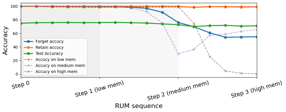
(a) low $\rightarrow$ med $\rightarrow$ high (Tow: 0.92, MIA gap: 0.059)

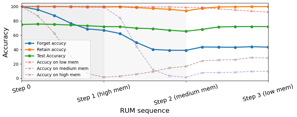
(b) high $\rightarrow$ med $\rightarrow$ low (ToW: 0.93, MIA gap: 0.022)

Figure 9: Analysis of sequence dynamics for two different orderings. We apply NegGrad+ RUM on CIFAR-100 dataset using ResNet-50 and show the accuracy on overall forget set (and each of its subsets), the retain set and test set after each step in the RUM sequence.

References

- Adebayo et al. [2018] Julius Adebayo, Justin Gilmer, Michael Muelly, Ian Goodfellow, Moritz Hardt, and Been Kim. Sanity checks for saliency maps. Advances in neural information processing systems, 31, 2018.
- Barbulescu and Triantafillou [2024] George-Octavian Barbulescu and Peter Triantafillou. To each (textual sequence) its own: Improving memorized-data unlearning in large language models. arXiv preprint arXiv:2405.03097 (to appear in ICML 2024), 2024.
- Bourtoule et al. [2021] Lucas Bourtoule, Varun Chandrasekaran, Christopher A Choquette-Choo, Hengrui Jia, Adelin Travers, Baiwu Zhang, David Lie, and Nicolas Papernot. Machine unlearning. In 2021 IEEE Symposium on Security and Privacy (SP), pages 141–159. IEEE, 2021.
- Carlini et al. [2019] Nicholas Carlini, Ulfar Erlingsson, and Nicolas Papernot. Distribution density, tails, and outliers in machine learning: Metrics and applications. arXiv preprint arXiv:1910.13427, 2019.
- Carlini et al. [2022a] Nicholas Carlini, Steve Chien, Milad Nasr, Shuang Song, Andreas Terzis, and Florian Tramer. Membership inference attacks from first principles. In 2022 IEEE Symposium on Security and Privacy (SP), pages 1897–1914. IEEE, 2022a.
- Carlini et al. [2022b] Nicholas Carlini, Matthew Jagielski, Chiyuan Zhang, Nicolas Papernot, Andreas Terzis, and Florian Tramer. The privacy onion effect: Memorization is relative. Advances in Neural Information Processing Systems, 35:13263–13276, 2022b.
- Cook and Weisberg [1982] R Dennis Cook and Sanford Weisberg. Criticism and influence analysis in regression. Sociological methodology, 13:313–361, 1982.
- Dwork [2006] Cynthia Dwork. Differential privacy. In International colloquium on automata, languages, and programming, pages 1–12. Springer, 2006.
- Fan et al. [2023] Chongyu Fan, Jiancheng Liu, Yihua Zhang, Dennis Wei, Eric Wong, and Sijia Liu. Salun: Empowering machine unlearning via gradient-based weight saliency in both image classification and generation. arXiv preprint arXiv:2310.12508, 2023.
- Fan et al. [2024] Chongyu Fan, Jiancheng Liu, Alfred Hero, and Sijia Liu. Challenging forgets: Unveiling the worst-case forget sets in machine unlearning. arXiv preprint arXiv:2403.07362, 2024.
- Feldman [2020] Vitaly Feldman. Does learning require memorization? a short tale about a long tail. In Proceedings of the 52nd Annual ACM SIGACT Symposium on Theory of Computing, pages 954–959, 2020.
- Feldman and Zhang [2020] Vitaly Feldman and Chiyuan Zhang. What neural networks memorize and why: Discovering the long tail via influence estimation. Advances in Neural Information Processing Systems, 33:2881–2891, 2020.
- Frankle and Carbin [2018] Jonathan Frankle and Michael Carbin. The lottery ticket hypothesis: Finding sparse, trainable neural networks. arXiv preprint arXiv:1803.03635, 2018.
- Ginart et al. [2019] Antonio Ginart, Melody Guan, Gregory Valiant, and James Y Zou. Making ai forget you: Data deletion in machine learning. Advances in neural information processing systems, 32, 2019.
- Golatkar et al. [2020] Aditya Golatkar, Alessandro Achille, and Stefano Soatto. Eternal sunshine of the spotless net: Selective forgetting in deep networks. In Proceedings of the IEEE/CVF Conference on Computer Vision and Pattern Recognition, pages 9304–9312, 2020.
- Goldblum et al. [2020] Micah Goldblum, Steven Reich, Liam Fowl, Renkun Ni, Valeriia Cherepanova, and Tom Goldstein. Unraveling meta-learning: Understanding feature representations for few-shot tasks. In International Conference on Machine Learning, pages 3607–3616. PMLR, 2020.
- Graves et al. [2021] Laura Graves, Vineel Nagisetty, and Vijay Ganesh. Amnesiac machine learning. In Proceedings of the AAAI Conference on Artificial Intelligence, volume 35, pages 11516–11524, 2021.
- Guo et al. [2019] Chuan Guo, Tom Goldstein, Awni Hannun, and Laurens Van Der Maaten. Certified data removal from machine learning models. arXiv preprint arXiv:1911.03030, 2019.
- Hayes et al. [2024] Jamie Hayes, Ilia Shumailov, Eleni Triantafillou, Amr Khalifa, and Nicolas Papernot. Inexact unlearning needs more careful evaluations to avoid a false sense of privacy. arXiv preprint arXiv:2403.01218, 2024.
- Izzo et al. [2021] Zachary Izzo, Mary Anne Smart, Kamalika Chaudhuri, and James Zou. Approximate data deletion from machine learning models. In International Conference on Artificial Intelligence and Statistics, pages 2008–2016. PMLR, 2021.
- Jagielski et al. [2022] Matthew Jagielski, Om Thakkar, Florian Tramer, Daphne Ippolito, Katherine Lee, Nicholas Carlini, Eric Wallace, Shuang Song, Abhradeep Thakurta, Nicolas Papernot, et al. Measuring forgetting of memorized training examples. arXiv preprint arXiv:2207.00099, 2022.
- Jiang et al. [2020] Ziheng Jiang, Chiyuan Zhang, Kunal Talwar, and Michael C Mozer. Characterizing structural regularities of labeled data in overparameterized models. arXiv preprint arXiv:2002.03206, 2020.
- Koh and Liang [2017] Pang Wei Koh and Percy Liang. Understanding black-box predictions via influence functions. In International conference on machine learning, pages 1885–1894. PMLR, 2017.
- Kurmanji et al. [2024] Meghdad Kurmanji, Peter Triantafillou, Jamie Hayes, and Eleni Triantafillou. Towards unbounded machine unlearning. Advances in Neural Information Processing Systems, 36, 2024.
- Liu et al. [2024] Jiancheng Liu, Parikshit Ram, Yuguang Yao, Gaowen Liu, Yang Liu, PRANAY SHARMA, Sijia Liu, et al. Model sparsity can simplify machine unlearning. Advances in Neural Information Processing Systems, 36, 2024.
- Ma et al. [2021] Xiaolong Ma, Geng Yuan, Xuan Shen, Tianlong Chen, Xuxi Chen, Xiaohan Chen, Ning Liu, Minghai Qin, Sijia Liu, Zhangyang Wang, et al. Sanity checks for lottery tickets: Does your winning ticket really win the jackpot? Advances in Neural Information Processing Systems, 34:12749–12760, 2021.
- Mattern et al. [2023] Justus Mattern, Fatemehsadat Mireshghallah, Zhijing Jin, Bernhard Schölkopf, Mrinmaya Sachan, and Taylor Berg-Kirkpatrick. Membership inference attacks against language models via neighbourhood comparison. arXiv preprint arXiv:2305.18462, 2023.
- Nguyen et al. [2022] Thanh Tam Nguyen, Thanh Trung Huynh, Phi Le Nguyen, Alan Wee-Chung Liew, Hongzhi Yin, and Quoc Viet Hung Nguyen. A survey of machine unlearning. arXiv preprint arXiv:2209.02299, 2022.
- Smilkov et al. [2017] Daniel Smilkov, Nikhil Thorat, Been Kim, Fernanda Viégas, and Martin Wattenberg. Smoothgrad: removing noise by adding noise. arXiv preprint arXiv:1706.03825, 2017.
- Thudi et al. [2022] Anvith Thudi, Gabriel Deza, Varun Chandrasekaran, and Nicolas Papernot. Unrolling sgd: Understanding factors influencing machine unlearning. In 2022 IEEE 7th European Symposium on Security and Privacy (EuroS&P), pages 303–319. IEEE, 2022.
- Toneva et al. [2018] Mariya Toneva, Alessandro Sordoni, Remi Tachet des Combes, Adam Trischler, Yoshua Bengio, and Geoffrey J Gordon. An empirical study of example forgetting during deep neural network learning. arXiv preprint arXiv:1812.05159, 2018.
- Triantafillou et al. [2023] Eleni Triantafillou, Fabian Pedregosa, Jamie Hayes, Peter Kairouz, Isabelle Guyon, Meghdad Kurmanji, Gintare Karolina Dziugaite, Peter Triantafillou, Kairan Zhao, Lisheng Sun Hosoya, Julio C. S. Jacques Junior, Vincent Dumoulin, Ioannis Mitliagkas, Sergio Escalera, Jun Wan, Sohier Dane, Maggie Demkin, and Walter Reade. Neurips 2023 - machine unlearning, 2023. URL https://kaggle.com/competitions/neurips-2023-machine-unlearning.
- Wang et al. [2022] Junxiao Wang, Song Guo, Xin Xie, and Heng Qi. Federated unlearning via class-discriminative pruning. In Proceedings of the ACM Web Conference 2022, pages 622–632, 2022.
- Warnecke et al. [2021] Alexander Warnecke, Lukas Pirch, Christian Wressnegger, and Konrad Rieck. Machine unlearning of features and labels. arXiv preprint arXiv:2108.11577, 2021.