On the Nonlinearity of Layer Normalization

Abstract

Layer normalization (LN) is a ubiquitous technique in deep learning but our theoretical understanding to it remains elusive. This paper investigates a new theoretical direction for LN, regarding to its nonlinearity and representation capacity. We investigate the representation capacity of a network with layerwise composition of linear and LN transformations, referred to as LN-Net. We theoretically show that, given $m$ samples with any label assignment, an LN-Net with only 3 neurons in each layer and $O(m)$ LN layers can correctly classify them. We further show the lower bound of the VC dimension of an LN-Net. The nonlinearity of LN can be amplified by group partition, which is also theoretically demonstrated with mild assumption and empirically supported by our experiments. Based on our analyses, we consider to design neural architecture by exploiting and amplifying the nonlinearity of LN, and the effectiveness is supported by our experiments.

1 Introduction

Layer normalization (LN) (Ba et al., 2016) is a ubiquitous technique in deep learning, enabling varies neural networks to train effectively. It was initially proposed to address the train-inference inconsistency problem of Batch Normalization (BN) (Ioffe & Szegedy, 2015) applied in the recurrent neural networks for Natural Language Processing (NLP) tasks. It then became the key component of Transformer (Vaswani et al., 2017) and its variants (Dai et al., 2019; Xiong et al., 2020; Dosovitskiy et al., 2021), spreading from NLP (Radford et al., 2021; Devlin et al., 2019; Raffel et al., 2020) to Computer Vision (CV) (Dosovitskiy et al., 2021; Carion et al., 2020; Cheng et al., 2022) communities. LN has got its firm position (Huang et al., 2023) in the evolution of neural architectures and is currently a basic layer in almost all the foundation models (Brown et al., 2020; Alayrac et al., 2022; Kirillov et al., 2023).

While LN is extensively used in practice, our theoretical understanding to it remains elusive. One main theoretical work for LN is its scale-invariant property, which is initially discussed in (Ba et al., 2016) to illustrate its ability in stabilizing training and is further extended in (Hoffer et al., 2018; Arora et al., 2019; Li & Arora, 2020) to consider its potential affects in optimization dynamics. Different from the previous work focusing on theoretical analyses of LN from the perspective of optimization, this paper investigates a new theoretical direction for LN, regarding to its nonlinearity and representation capacity.

We mathematically demonstrate that LN is a nonlinear transformation. We highlight that LN might be a nonlinear transformation by intuition, but there is no work, to our best knowledge, demonstrating it. Our demonstration is based on the defined lower bound named LSSR (Definition 2). The LSSR will not be broken under any linear transformation by definition, but we show that a linear neural network combined with LN can break the LSSR. Therefore, LN has nonlinearity. We also show that an LN-Net, which is a layerwise composition of linear and LN transformations, has nonlinearity.

One interesting question is that how powerful the nonlinear of an LN-Net is in theory. We theoretically show that, given $m$ samples with any label assignment, an LN-Net with only 3 neurons in each layer and $O(m)$ LN layers can correctly classify them. We further show the lower bound of the VC dimension of an LN-Net. In particular, given an LN-Net with width only 3 neurons in each layer and $L$ LN layers, its VC dimension is lower bounded by $L+2$. These results show that LN-Net has great representation capacity in theory, implying the possibility that a network with linear and LN layer only can work well in practice.

We further investigate how to amplify and exploit the nonlinearity of LN. We find that Group based LN (LN-G)—which divides neurons of a layer into groups and perform LN in each group in parallel—has stronger nonlinearity than the naive LN countpart. This is also theoretically demonstrated with mild assumption and empirically supported by our comprehensive experiments. We also consider practical scenario, where we replace LN with LN-G on Transformer and ViT, since we believe the amplified nonlinearity can benefits the models. The preliminary results show the potentiality of this design in neural architecture.

2 Preliminary and Notation

We use a lowercase letter $x\in\R$ to denote a scalar, boldface lowercase letter $\rvx\in\R^{d}$ for a vector and boldface uppercase letter for a matrix $\mX\in\R^{d\times m}$, where $\R$ is the set of real-valued numbers, and $d,m$ are positive integers.

Neural Network.

Given the input $\rvx$, a classical neural network $f_{\theta}(\rvx)$ is typically represented as a layer-wise linear and nonlinear transformation:

$$\vh^{(l)} = \mW^{(l)}\rvx^{(l-1)}+\vb^{(l)},$$ (1)

$$\rvx^{(l)} = \phi(\vh^{(l)}),~{}~{}~{}l=1,...,L,$$ (2)

where $\mathbf{\theta}=\{(\mW^{(l)},\vb^{(l)}),l=1,\cdots,L\}$ are learnable parameters, $\rvx^{(0)}=\rvx$, $\mW^{(l)}\in\R^{d_{l}\times d_{l-1}}$, $\vb^{(l)}\in\R^{d_{l}}$ and $d_{l}$ indicates the number of neurons in the $l$-th layer. We set $\rvx^{(L)}=\vh^{(L)}$ as the output of the network $f_{\theta}(\rvx)$ to simplify denotations. A neural network without nonlinear transformation $\phi(\cdot)$ (Eqn. 2) is referred to as a linear neural network, which is still a linear transformation in native.

Layer Normalization.

Layer Normalization (LN) is an essential layer in modern deep neural networks mainly for stabilizing training. Given a single sample of layer input $\rvx=[x^{(1)},x^{(2)},\cdots,x^{(d)}]\in\mathbb{R}^{d}$ with $d$ neurons in a neural network, LN standardizes $\rvx$ within the neurons as :

$$\hat{x}^{(j)}=LN(x^{(j)})=\frac{x^{(j)}-\mu}{\sigma},~{}~{}j=1,2,\cdots,d,$$ (3)

where $\mu=\frac{1}{d}\sum\limits_{i=1}^{d}x^{(j)}$ and $\sigma=\sqrt{\frac{1}{d}\sum\limits_{i=1}^{d}(x^{(j)}-\mu)^{2}}$ are the mean and variance for each sample, respectively. The standardization operation can be viewed as a combination of centering and scaling operations. Centering projects $\rvx$ onto the hyperplane $\{\rvx\in\R^{d}:x^{(1)}+\cdots+x^{(d)}=0\}$, by $\tilde{\rvx}=(\mI-\frac{1}{d}\bm{1}_{d}\bm{1}_{d}^{\top})\rvx$. Scaling projects $\tilde{\rvx}$ onto the sphere $\{\rvx\in\R^{d}:[x^{(1)}]^{2}+\cdots+[x^{(d)}]^{2}=d\}$, by $\hat{\rvx}=\sqrt{d}\tilde{\rvx}/\|\tilde{\rvx}\|_{2}$. We thus also call scaling as Spherical Projection (SP), from the geometric perspective. Note that SP is the only operation for normalization in RMSNorm (Zhang & Sennrich, 2019).

Sum of Squares.

Sum of Squares (SS) (Fisher, 1970) is a statistical concept that measures the variability or dispersion within a set of data. Denote $m$ samples from class $c$ as $\rvx_{c1},\cdots,\rvx_{cm}\in\R^{d}$, represented as a matrix $\mX_{c}=[\rvx_{c1},\cdots,\rvx_{cm}]$, then SS of $\mX_{c}$ is defined as

$$SS(\mX_{c})=\sum_{i=1}^{m}\left\|\rvx_{ci}-\bar{\rvx}_{c}\right\|^{2},$$ (4)

where $\bar{\rvx}_{c}=(\rvx_{c1}+\cdots+\rvx_{cm})/m$.

3 The Existence of Nonlinearity in LN

In this section, we define Sum of Squares Ratio (SSR) and its linear invariant lower bound named LSSR. We then show that LN can break the boundary of SSR and plays a role in nonlinear representation.

3.1 Linear Invariant Lower Bound

We take binary classification for simplifying discussion. Let $\mX_{c}=[\rvx_{c1},\cdots,\rvx_{cm}]$ represents $m$ samples in $\R^{d}$ from the corresponding class $c\in\{1,2\}$, and $[\mX_{1},\mX_{2}]\in\R^{d\times 2m}$ represents all the samples together.

Definition 1.

(SSR.) Given $SS([\mX_{1},\mX_{2}])\neq 0$, the Sum of Squares Ratio (SSR) between $\mX_{1}$ and $\mX_{2}$ is defined as

$$SSR(\mX_{1},\mX_{2})=\frac{SS(\mX_{1})+SS(\mX_{2})}{SS([\mX_{1},\mX_{2}])}.$$ (5)

It is easy to demonstrate that $SSR(\mX_{1},\mX_{2})\in[0,1]$. SSR can be an indicator to show how easy the samples in the Euclidean space from different classes can be separated. I.e., the smaller SSR is, the more easily $\mX_{1}$ and $\mX_{2}$ are to be separated with Eulcidean distance as a measurement in most cases. Based on SSR, we further define its lower bound under any linear transformation as follows.

Definition 2.

(LSSR.) The Linear SSR (LSSR) between $\mX_{1}$ and $\mX_{2}$ is defined as

$$LSSR(\mX_{1},\mX_{2})=\inf_{\varphi\in\sD_{\varphi}(d)}SSR(\varphi(\mX_{1}),\varphi(\mX_{2})),$$ (6)

where $\sD_{\varphi}(d)$ is the set of all linear functions defined on $\R^{d}$.

By definition, LSSR is the lower bound of SSR under any linear transformation. LSSR can be an indicator to show how easy the samples from different classes can be linearly separated. We provide illustrative examples in Appendix A for details. In the following proposition, we show a linear neural network can not break LSSR.

Proposition 1.

Given $\mX_{1},\mX_{2}\in\R^{d_{0}\times m}$ and a linear neural network represented as $\tilde{\varphi}=\varphi_{1}\circ\cdots\circ\varphi_{L}$, where $\varphi_{l}:\R^{d_{l-1}}\to\R^{d_{l}},(l=1,\cdots,L)$ are all linear transformations as shown in Eqn. 1, we have that

$$SSR(\tilde{\varphi}(\mX_{1}),\tilde{\varphi}(\mX_{2}))\geq LSSR(\mX_{1},\mX_{2}).$$ (7)

Proposition 1 is easily proved by the definition of LSSR, since we have $\tilde{\varphi}\in\sD_{\varphi}(d_{0})$. Proposition 1 implies that the SSR will not break the lower bound if we use an arbitrary linear neural network as a representation transformation over the samples. One interesting question is that whether a linear neural network combined with LN can break the lower bound of SSR. If Yes, we can show that LN has nonlinearity.

3.2 Break the Lower Bound of SSR with LN

Here, we focus on the linear neural network combined with LN. To state more precisely, we denote LN-Net as follows.

Definition 3.

(LN-Net.) The LN-Net $f_{\theta}(\rvx)$ is defined as layer-wise composition of linear and LN transformation:

$$\vh^{(l)} = \mW^{(l)}\rvx^{(l-1)}+\vb^{(l)},~{}~{}l=1,...,L,$$ (8)

$$\rvx^{(l)} = LN(\vh^{(l)}),~{}~{}~{}l=1,...,L-1,$$

where $\mathbf{\theta}=\{(\mW^{(l)},\vb^{(l)}),l=1,...,L\}$ are learnable parameters, $\rvx^{(0)}=\rvx$ and $LN(\cdot)$ denotes the LN operation. We set $\rvx^{(L)}=\vh^{(L)}$ as the output of the network $f_{\theta}(\rvx)$ to simplify denotations.

We first provide a tractable method to calculate LSSR, stated by the following proposition.

Proposition 2.

Given $\mX_{1},\mX_{2}\in\R^{d\times m}$, we denote $\mM=\sum\limits_{c=1}^{2}\sum\limits_{i=1}^{m}(\rvx_{ci}-\bar{\rvx}_{c})(\rvx_{ci}-\bar{\rvx}_{c})^{\top}$, and $\mN=\sum\limits_{c=1}^{2}\sum\limits_{i=1}^{m}(\rvx_{ci}-\bar{\rvx})(\rvx_{ci}-\bar{\rvx})^{\top}$, where $\bar{\rvx}=(\bar{\rvx}_{1}+\bar{\rvx}_{2})/2$. Supposing that $\mN$ is reversible, we have

$$LSSR(\mX_{1},\mX_{2})=\lambda^{*},$$ (9)

and correspondingly,

$$LSSR(\mX_{1},\mX_{2})=SSR((\vu^{*})^{\top}\mX_{1},(\vu^{*})^{\top}\mX_{2}),$$ (10)

where $\lambda^{*}$ and $\vu^{*}$ are the minimum eigenvalue and corresponding eigenvector of $\mN^{-1}\mM$.

The proof of Proposition 2 are shown in Appendix B. Based on Proposition 2, we further define $f_{SSR}(t)$ as

$$f_{SSR}(t)=\begin{cases}LSSR(\mX_{1},\mX_{2}),&t=0,\\ SSR(\bar{\psi}(t;\mX_{1}),\bar{\psi}(t;\mX_{2})),&t\neq 0,\end{cases}$$ (11)

where $\bar{\psi}(t;\rvx_{ci})=\bm 1^{\top}\bar{\varphi}(t;\rvx_{ci})/\|\bar{\varphi}(t;\rvx_{ci})\|_{2}$, $\bar{\varphi}(t;\rvx_{ci})=[(\vu^{*})^{\top}\rvx_{ci}t,1]^{\top}$ and $t\in\R$. We point out that $f_{SSR}(t)$ is derivable at $t=0$, and $f_{SSR}^{\prime}(0)$ is only decided by $\mX_{1}$ and $\mX_{2}$, which is proved in Appendix C.

Based on the definition of $f_{SSR}(t)$, we show that LN-Net can decrease the LSSR as stated by the following theorem.

Theorem 1.

Let $\psi=\varphi_{1}\circ LN(\cdot)\circ\varphi_{2}$, performing over the input $\mX_{1},\mX_{2}\in\R^{d\times m}$. If $f_{SSR}^{\prime}(0)\neq 0$ , we can always find suitable linear functions $\varphi_{1}$ and $\varphi_{2}$, such that

$$SSR(\psi(\mX_{1}),\psi(\mX_{2}))<LSSR(\mX_{1},\mX_{2}).$$ (12)

The proof of Theorem 1 requires complicated derivation. Please refer to Appendix C for details. Note that LN-Net is a more general form of $\psi$ in Theorem 1, which implies that LN-Net can break the lower bound of SSR.

Based on Theorem 1, we can obtain the following statement. We deduce that LN is a nonlinear transformation.

Corollary 1.

LN is a nonlinear transformation.

Proof.

We assume that $LN(\cdot)$ is a linear transformation. We thus have LN-Net is also a linear transformation. Based on Proposition 1, we have LN-Net can not break LSSR. This contradicts Theorem 1. Therefore, $LN(\cdot)$ must be a nonlinear transformation. ∎

Summary.

In this section, we mathematically show that LN is a nonlinear transformation, and LN-Net is a network with nonlinearity. One interesting question is that how powerful the nonlinearity of an LN-Net is in theory. We will discuss about it in the following section.

4 Capacity of a Network with LN

In this section, we apply LN-Net to classify $m$ samples with any label assignment. To prove the existence of such LN-Net, we propose Projection Merge Algorithm (PMA) and Parallelization Breaking Algorithm (PBA) to help find the parameters of the LN-Net.

4.1 LN for Xor Classification

To understand PMA intuitively, we use Spherical Projection (SP) rather than LN at the beginning. But we replace SP with LN and linear layers back in the end, according to the lemma as follows.

Lemma 1.

Denote $LN(\cdot)$ as the LN operation in $\R^{d}(d\geq 3)$, and $SP(\cdot)$ as the SP operation in $\R^{d-1}$. We can find some linear transformations $\hat{\varphi}_{1}$ and $\hat{\varphi}_{2}$, such that

$$SP(\cdot)=\hat{\varphi}_{1}\circ LN(\cdot)\circ\hat{\varphi}_{2}.$$ (13)

The proof of Lemma 1 is shown in Appendix C. And we can easily obtain the following corollary.

Corollary 2.

$SP(\cdot)$ can be represented by an LN-Net.

Taking xor classification as an example, we primarily show how we use LN-Net to classify linearly inseparable samples.

(a) Initial input.

(b) Rotation.

(c) Linear projection.

(d) Spherical projection.

(e) Linear projection.

Figure 1: Solution to the Xor Classification. To begin with, we rotate them by $45^{\circ}$, as shown in Figure 1(b). Then we vertically project them onto $y=0.5$, as shown in Figure 1(c). Next, we spherically project them onto the circle $x^{2}+y^{2}=1$, as shown in Figure 1(d). Finally, we horizontally project them onto $x=0$, as shown in Figure 1(e). Now we have classified the two classes.

As shown in Figure 1(a), $(0,0),(1,1)$ and $(0,1),(1,0)$ belong to different classes. Obviously, the two classes are not linearly separable. We can classify them with SP and linear transformations only, please refer to the demonstration in Figure 1 for details.

By Lemma 1, replace SP with LN-Net. Therefore, we can construct an LN-Net according to the operations in Figure 1, and then classify the xor samples.

More generally, we discuss binary classification in Section 4.2 and multi-class classification in Section 4.3.

4.2 LN for Binary Classification

Theorem 2.

Given $m$ samples with any binary label assignment in $\{0,1\}$, there always exists an LN-Net with only $3$ neurons per layer and $O(m)$ LN layers can correctly classify them.

To prove Theorem 2, we represent the LN-Net with SP and linear layers. Then we design an algorithm to help compute the parameters according to the input. We hence get an LN-Net with proper parameters to classify the samples. The proof is shown as follows.

We represent an LN-Net as

$$f_{\theta}(\cdot)=\varphi_{1}\circ LN(\cdot)\circ\varphi_{2}\circ\cdots\circ\varphi_{L-1}\circ LN(\cdot)\circ\varphi_{L},$$ (14)

where $\varphi_{1},\cdots,\varphi_{L}$ denote the linear layers, and $LN(\cdot)$ denotes the LN layers. For convenience, we replace LN with SP temporarily.

Proposition 3.

The LN-Net $f_{\theta}(\cdot)$ in 14 can be represented by SP and linear layers equivalently.

Proof.

Since each $LN(\cdot)$ acts on $\R^{3}$, by Lemma 1, we can construct a $2$-dimensional $SP(\cdot)=\hat{\varphi}_{1}\circ LN(\cdot)\circ\hat{\varphi}_{2}$. Define each $\varphi_{l}$ in Theorem 2 as

$$\varphi_{l}=\begin{cases}\varphi_{l}^{(1)}\circ\varphi_{l}^{(2)}\circ\hat{\varphi}_{1},&l=1,\\ \hat{\varphi}_{2}\circ\varphi_{l}^{(1)}\circ\varphi_{l}^{(2)}\circ\hat{\varphi}_{1},&1<l<L,\\ \hat{\varphi}_{2}\circ\varphi_{l}^{(1)},&l=L,\end{cases}$$ (15)

where $\varphi_{l}^{(1)}$ and $\varphi_{l}^{(2)}$ are both linear functions. By 15 and Lemma 1, we can rewrite $f_{\theta}(\cdot)$ as

$$\tilde{f}_{\theta}(\cdot)=\varphi_{1}^{(1)}\circ\varphi_{1}^{(2)}\circ SP(\cdot)\circ\varphi_{2}^{(1)}\circ\cdots\circ SP(\cdot)\circ\varphi_{L}^{(1)},$$ (16)

namely, $f_{\theta}(\cdot)$ can be represented by SP and linear layers equivalently. ∎

Hereafter, we consider to compute the parameters of $\tilde{f}_{\theta}(\cdot)$. Specifically, for each layer, we denote

$$\begin{cases}\varphi_{l}^{(1)}:\mX^{(l-1)}\mapsto\mP^{(l)},&1\leq l\leq L;\\ \varphi_{l}^{(2)}:\mP^{(l)}\mapsto\mH^{(l)},&1\leq l\leq L-1;\\ SP(\cdot):\mH^{(l)}\mapsto\mX^{(l)},&1\leq l\leq L-1.\end{cases}$$ (17)

Besides, the input of $\tilde{f}_{\theta}(\cdot)$ is $\mX^{(0)}=[\rvx_{1}^{(0)},\cdots,\rvx_{m}^{(0)}]$, and the output is $\mP^{(L)}$. Now we construct $\tilde{f}_{\theta}(\cdot)$ step by step.

We denote that for each $\mP^{(l)},(l=1,\cdots,L)$, these points are on the $x$-axis, namely $\vp_{k}^{(l)}=[p_{k}^{(l)},0]^{\top},(k=1,\cdots,m)$. To get $\mP^{(1)}$, we apply $\varphi_{1}^{(1)}$ for initialization as below.

Proposition 4.

For any input $\mX^{(0)}$, we can find some $\vu$, such that

$$\varphi_{1}^{(1)}:\rvx_{k}^{(0)}\mapsto\vp_{k}^{(1)}=[\vu^{\top}\rvx_{k}^{(0)},0]^{\top},$$ (18)

where $\vp_{i}^{(1)}\neq\vp_{j}^{(1)}$ if $\rvx_{i}^{(0)}\neq\rvx_{j}^{(0)}$.

Proposition 4 parameterizes $\varphi_{1}^{(1)}$ and initializes $\mP^{(1)}$ onto the $x$-axis, without merging different points. Please refer to Appendix LABEL:section:proofofAlgorithms for the proof.

As for other linear functions, the suitable parameters are generated from the Projection Merge Algorithm, as shown in Algorithm 1.

0:  The initial input $\mP^{(1)}$.

0:  The final output $\mP^{(L)}$.

1:  $l\leftarrow 1$;

2:  $\sP\leftarrow\{\vp_{1}^{(l)},\vp_{2}^{(l)},\cdots,\vp_{m}^{(l)}\}$;

3:  while $\sP\neq\emptyset$ do

4:     $i\leftarrow\arg\min\limits_{k}\{p_{k}^{(l)}:\vp_{k}^{(l)}\in\sP\}$;

5:     $\sJ_{i}\leftarrow\{\vp_{j}^{(l)}\in\sP:\vp_{j}^{(l)}\neq\vp_{i}^{(l)},y_{j}=y_{i}\}$;

6:     if $\sJ_{i}\neq\emptyset$ then

7:        $j\leftarrow\arg\min\limits_{k}\{p_{k}^{(l)}:\vp_{k}^{(l)}\in\sJ_{i}\}$;

8:        for $k\leftarrow 1$ to $m$ do

9:           $\vh_{k}^{(l)}\leftarrow\vp_{k}^{(l)}-\mat{p_{i}^{(l)}+p_{j}^{(l)}\par\addvspace{-\parskip}\ignorespaces p_{i}^{(l)}-p_{j}^{(l)}}/2$;

10:           $\rvx_{k}^{(l)}\leftarrow\vh_{k}^{(l)}/\|\vh_{k}^{(l)}\|$;

11:           $\vp_{k}^{(l+1)}\leftarrow\mat{0&1\par\addvspace{-\parskip}\ignorespaces 00}\rvx_{k}^{(l)}$;

12:        end for

13:        $l\leftarrow l+1$;

14:        $\sP\leftarrow\{\vp_{1}^{(l)},\vp_{2}^{(l)},\cdots,\vp_{m}^{(l)}\}$;

15:     else

16:        remove $\vp_{j}^{(l)}$ from $\sP$, as long as $\vp_{j}^{(l)}=\vp_{i}^{(l)}$;

17:     end if

18:  end while

19:  return $\mP^{(l)}$;

Algorithm 1 Projection Merge Algorithm

In Algorithm 1, $\mP^{(L)}$ is the output, as well as that of $\tilde{f}_{\theta}(\cdot)$. Factually, by Algorithm 1, we get each $\mP^{(l)}$ in a recursive way. For the case $\sJ_{i}\neq\emptyset$, we take $5$ points as an example to show how we get $\mP^{(l+1)}$ from $\mP^{(l)}$ in Figure 2.

(a) Translation.

(b) Spherical projection.

(c) Linear projection.

Figure 2: Get $\mP^{(l+1)}$ from $\mP^{(l)}$ geometrically. In Figure 2(a), $\mP^{(l)}$ is shown as the bars on the $x$-axis. At first, find the leftmost point, namely $\vp_{1}^{(l)}$. Then we find another point with the same label as $\vp_{1}^{(l)}$, but right of $\vp_{1}^{(l)}$, choose the leftmost one, namely $\vp_{4}^{(l)}$. Afterwards, shift all the points up by $(p_{4}^{(l)}-p_{1}^{(l)})/2$, and left by $(p_{4}^{(l)}+p_{1}^{(l)})/2$, then we get $\mH^{(l)}$, as shown in Figure 2(a). Next, spherically project $\mH^{(l)}$ onto the unit circle and get $\mX^{(l)}$, shown as ’+’s in Figure 2(b). Finally merge the points in $\mX^{(l)}$ by their ordinates, as the new abscissas of $\mP^{(l+1)}$, and take $0$ as the new ordinates of $\mP^{(l+1)}$, as shown in Figure 2(c). Now, we have $\mP^{(l+1)}$.

As for the case $\sJ_{i}=\emptyset$, it indicates that all points with the same label as $\vp_{i}^{(l)}$ are merged together. Therefore, we remove them from $\sP$, and choose the leftmost point from the remaining $\sP$, until $\sP=\emptyset$.

Based above, we give the properties of each layer as follows.

Proposition 5.

For each layer, $\varphi_{l}^{(1)}(2\leq l\leq L)$ only merges points with the same label. Nevertheless, $\varphi_{1}^{(1)},SP(\cdot)$ and $\varphi_{l}^{(2)}(1\leq l\leq L-1)$ do not merge any points.

Please refer to Appendix LABEL:section:proofofAlgorithms for the proof of Proposition 5.

By Proposition 5, we figure out that Algorithm 2 will only merge points with the same label. Besides, we find that from $\mP^{(l)}$ to $\mP^{(l+1)}$, the number of different points will decrease at least $1$. Since the input is $m$ different points from two classes, we merge at most $m-2$ times by Algorithm 1, we thus have $L-1\leq m-2$.

By Algorithm 1, we can construct other linear functions with exact parameters as follows.

$$\begin{cases}\varphi_{l}^{(1)}:\rvx_{k}^{(l-1)}\mapsto\mat{0&1\\ 0&0}\rvx_{k}^{(l-1)},&1<l\leq L,\\ \varphi_{l}^{(2)}:\vp_{k}^{(l)}\mapsto\vp_{k}^{(l)}-\mat{p_{i}^{(l)}+p_{j}^{(l)}\\ p_{i}^{(l)}-p_{j}^{(l)}}/2,&1\leq l<L.\end{cases}$$ (19)

Therefore, $\tilde{f}_{\theta}(\cdot)$ with the parameters in 18 and 19 can classify the samples $\mX^{(0)}$. Besides, the LN-Net in 14 with depth $L-1=O(m)$ can also classify the $m$ samples. We hence have proved Theorem 2.

Our results above are based on an LN-Net with $3$ neurons each layer. Furthermore, we can generalize PMA for a wider neural network, but it is much more complex. Please refer to Appendix LABEL:section:proofofAlgorithms for more details.

Based on Theorem 2, we can easily obtain the following corollary related to VC dimension (Bartlett et al., 1998) of an LN-Net.

Corollary 3.

Given an LN-Net $f_{\theta}(\cdot)$ with width 3 and depth $L$, its VC dimension $VCdim(f_{\theta}(\cdot))$ is lower bounded by $L+2$.

4.3 LN for Multi-class Classification

Theorem 3.

Given $m$ samples with any binary label assignment, there always exists an LN-Net with only $3$ neurons per layer and $O(m)$ LN layers can correctly classify them.

Applying Algorithm 1 for a multi-class classification may confuse two samples with different labels. We thus introduce Parallelization Breaking Algorithm to avoid such confusion. Besides, we can also construct an LN-Net to classify the samples. The detailed analysis and proof are as below.

To begin with, we are concerned about whether Algorithm 1 applies to multi-class classification—the answer is Not. Based on Figure 2(c), we recolor $\rvx_{3}^{(l)}$ red, as shown in Figure 3. When we merge $\rvx_{1}^{(l)}$ and $\rvx_{4}^{(l)}$, $\rvx_{2}^{(l)}$ and $\rvx_{3}^{(l)}$ will be merged in the meanwhile. In other words, the algorithm will confuse them to be in the same class. Proposition 6 indicates the necessary condition for such confusion.

Figure 3: The case of confusion in the merging process.

Proposition 6.

Confusion refers to merging two points with different labels. If confusion happens when we project $\mX^{(l+1)}$ onto the $y$-axis, there must be a parallelogram consisting of four different points in $\mP^{(l)}$.

In reverse, if there is no parallelograms in $\mP^{(l)}$, confusion will never happen when applying Algorithm 1. Please refer to Appendix LABEL:section:proofofAlgorithms for the proof of Proposition 6.

To avoid such confusion, we propose Parallelization Breaking Algorithm (PBA) as follows.

0:  $\mP^{(l)}$, $\vu_{l}$ (got by Proposition 7).

0:  $\hat{\mP}^{(l)}$.

1:  for $k\leftarrow 1$ to $m$ do

2:     $\tilde{\vp}_{k}^{(l)}=SP(\vp_{k}^{(l)}+[0,1]^{\top})$;

3:     $\hat{\vp}_{k}^{(l)}=[\vu_{l}^{\top}\tilde{\vp}_{k}^{(l)},0]^{\top}$;

4:  end for

5:  return $\hat{\mP}^{(l)}$;

Algorithm 2 Parallelization Breaking Algorithm

Proposition 7.

We can always find $\vu_{l}\in\R^{2}$ for Algorithm 2, such that there is no parallelograms in $\hat{\mP}^{(l)}$, and no points merged in the algorithm.

Please refer to Appendix LABEL:section:proofofAlgorithms for the proof of Proposition 7.

PBA helps us transform $\mP^{(l)}$ to $\hat{\mP}^{(l)}$, based on which confusion will never happen. For multi-class classification, we insert PBA between $\varphi_{l}^{(1)}$ and $\varphi_{l}^{(2)}$ in 16, then given $m$ samples with any label assignment, $\tilde{f}_{\theta}(\cdot)$ with PBA can classify them. Based above, we replace SP with LN and linear layers in $\tilde{f}_{\theta}(\cdot)$ with PBA, and then merge the adjacent linear layers. We figure out $\tilde{f}_{\theta}(\cdot)$ with PBA is also an LN-Net. We point out that the depth of this LN-Net is no more than $2m$. We hence have proved Theorem 3.

Summary.

In this section, we show that LN-Net also has powerful capacity in theory. Our theoretical results show that an LN-Net with width $3$ and depth $O(m)$ is able to classify given $m$ samples with any label assignment. We see an LN-Net performing over $3$ neurons can introduce nonlinearity. One question is that whether the nonlinearity of an LN-Net with $d>3$ neurons can be amplified, if we group neurons and perform LN in each group in parallel? We answer it in the following section.

5 Amplify and Exploit the Nonlinearity of LN

5.1 Comparison of Nonlinearity

In this part, we first define a measurement over the Hessian matrix to compare the magnitude of the nonlinearity. We then show the Group based LN (LN-G)—which divides neurons of a layer into groups and perform LN in each group in parallel—has stronger nonlinearity than the naive LN countpart.

Hessian of Linear Function.

Given a twice differential function $f(\rvx):\R^{d}\to\R$, we focus on its Hessian Matrix $\nabla^{2}f(\rvx)$. If $f(\rvx)$ is a linear function, we have $\nabla^{2}f(\rvx)\equiv\mO$. More generally, suppose that $\varphi:\R^{d}\to\R^{d}$ is a linear transformation, we define $\varphi(\rvx)=\mat{\varphi_{1}(\rvx),\cdots,\varphi_{d}(\rvx)}^{\top}$, and each $\varphi_{i}(\rvx):\R^{d}\to\R$ is a linear function, namely each Hessian matrix $\nabla^{2}_{\rvx}\varphi_{i}(\rvx)=\mO$.

Measurement of Nonlinearity.

Given a twice differential function $f:\R^{d}\to\R^{d}$ and $\vy=f(\rvx)$. Denote $\vy=[y_{1},\cdots,y_{d}]^{\top}$ and $\rvx=[x_{1},\cdots,x_{d}]^{\top}$. We define $\mathcal{H}(f;\rvx)$ as an indicator to describe the Hessian information of $f:\R^{d}\to\R^{d}$ as

$$\mathcal{H}(f;\rvx)=\sum_{i=1}^{d}\left\|\pf{{}^{2}y_{i}}{\rvx^{2}}\right\|_{F}^{2},$$ (20)

where each $\displaystyle\pf{{}^{2}y_{i}}{\rvx^{2}}$ is a Hessian matrix.

We use the Frobenius norm rather than the operator norm, For easier calculations. Note that $\mathcal{H}(f;\rvx)\geq 0$, and $\mathcal{H}(f;\rvx)=0$ if and only if $f$ is a linear function. We thus assume that the larger $\mathcal{H}(f;\rvx)$ is, the more nonlinearity $f$ contains.

Amplifying Nonliearity by Group.

Denote $\psi_{G}(g;\cdot)$ as Group based LN (LN-G) on $\R^{d}$ with group number $g$, and $\psi_{L}(\cdot)$ as LN on $\R^{d}$. Compare LN with LN-G, the result is shown in Proposition 8.

Proposition 8.

Given $g\leq d/3$, we have

$$\frac{\mathcal{H}(\psi_{G}(g;\cdot);\rvx)}{\mathcal{H}(\psi_{L}(\cdot);\rvx)}\geq 1.$$ (21)

Specifically, when $g=d/4$, we figure out that

$$\frac{\mathcal{H}(\psi_{G}(g;\cdot);\rvx)}{\mathcal{H}(\psi_{L}(\cdot);\rvx)}\geq\frac{d}{8}.$$ (22)

Proposition 8 shows that LN-G can amplify the nonliearity of LN by using appropriated group number. Compared with LN, when $d$ is larger, LN-G shows more nonlineaity. Please refer to Appendix LABEL:section:proofofhessian for the proof. Besides, we generalize our discussion about $\mathcal{H}$ to the typical activation function ReLU, please refer to Appendix LABEL:section:proofofhessian for more details.

One limit of the result above is the assumption, that $\mathcal{H}(f;\rvx)$ is a good indicator for measuring nonlinearity, is from the intuition and can not be well verified. In the subsequent experiments, we empirically show that LN-G indeed can amplify the nonlinearity of LN.

5.2 Comparison of Representation Capacity by Fitting Random Labels

In this part, we follow the non-parametric randomization tests fitting random labels (Zhang et al., 2017) to empirically verify the nonlinearity of LN, and to further compare the representational capacity of LN-Net with different groups for LN-G. The experiments are conducted on CIFAR-10 and MNIST with random label assigned (CIFAR-10-RL and MNIST-RL). We evaluate the classification accuracy on the training set after the model is trained, which indicates that the capacity of models in fitting dataset empirically. We only provide essential components of the experimental setup; for more details, please refer to the Appendix LABEL:section:experiments.

Verify the Nonlinearity of LN.

We conduct experiments on linear neural network and LN-Net with 256 neurons in each layer and various depths. We first train sufficiently a linear classifier and obtain the (nearly) upper bound accuracy (18.51 % on CIFAR-10 -RL and 15.38% on MNIST-RL). To rule out the influence in optimization difficulty, we train the linear neural network and LN-Net with various configurations, including different learning rates and (with or without) residual connection. We report the best result from all configurations, as shown in Figure 4.

We observe that linear neural network cannot break the bound of linear classifier on all datasets, while LN-Net can reach the accuracy of 55.85% on CIFAR-10-RL and 19.44% on MNIST-RL, which is much better than the linear classifier. This result also verifies that LN has nonlinearity empirically. Besides, we observe that LN-Net obtains better performance in general as the depth increases (namely more LN layers and greater nonlinearity). We note that an LN-Net without sufficient depth does not break the bound of linear classifier on MNIST-RL. The reasons leading to this phenomenon are likely to be that: 1) MNIST-RL are more difficult to train, compare to CIFAR-10-RL; 2) LN-Nets have a non-convex optimization landscape and we cannot ensure the weight learned to be the optimal point, given fixed training epochs.

We also conduct experiments with Batch Normalization (BN) (Ioffe & Szegedy, 2015), where we replace LN with BN in LN-Net. We find that BN cannot break the bound of linear classifier on all datasets, like linear neural network. This preliminary result is interesting, which shows the potential advantage of LN over BN, in terms of the representation capacity.

(a) CIFAR-10-RL.

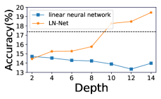
(b) MNIST-RL.

Figure 4: Results of linear neural network and LN-Net on fitting random label. The black dashed line represents the upper bound accuracy of linear classifier. (a) Results on CIFAR-10-RL; (b) Results on MNIST-RL.

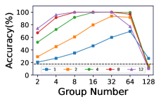
(a) Accuracy on CIFAR-10-RL.

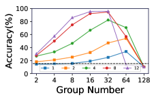
(b) Accuracy on MNIST-RL.

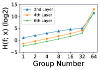
(c) $\mathcal{H}(f;\rvx)$ on CIFAR-10-RL.

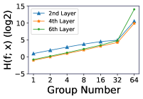
(d) $\mathcal{H}(f;\rvx)$ on MNIST-RL.

Figure 5: Results of LN-Net using LN-G. We vary the group number $g$ and show the training accuracy and $\mathcal{H}(f;\rvx)$. (a) Training accuracy on CIFAR-10-RL; (b) Training accuracy on MNIST-RL; (c)$\mathcal{H}(f;\rvx)$ on CIFAR-10-RL;(d) $\mathcal{H}(f;\rvx)$ on MNIST-RL. The black dashed line in (a) and (b) has the same meaning as that in Figure 4.

Amplifying the Nonlinearity using Group.

We conduct experiments on LN-Net with $d=256$ neurons in each layer and various depths. We replace LN in LN-Net with LN-G and also vary the group number $g$. We train LN-Net with various learning rates and report the best training accuracy on CIFAR-10-RL and MNIST-RL, as shown in Figure 5.

We observe that some LN-Net with LN-G (e.g., depth = 8 and $g=32$) can perfectly classify all the random labels on CIFAR-10-RL and MNIST-RL, which suggests that LN-G can amplify the nonlinearity of LN by using group, as stated in Proposition 8. We also observe that an LN-Net with appropriate group number (e.g, $g=32$) can obtain better performance, as the depth increases. Besides, an LN-Net has better performance in general with larger group number, along the group number is not too much (relative to the number of neurons). E.g, An LN-Net has significantly degenerated performance when $g=128$, due to $d/g=2<3$ that go against the premise in Proposition 8.

We also calculate $\mathcal{H}(f;\rvx)$ in certain layers and show how $\mathcal{H}(f;\rvx)$ varies as the group number increases in Figure 5 (c) and (d). $\mathcal{H}(f;\rvx)$ is calculated by averaging over 1000 samples in our experiments. We find $\mathcal{H}(f;\rvx)$ increases as the group number of LN-G increases, which matches our theoretical analyses in Section 5.1.

5.3 Inspiration for Neural Architecture Design

In this part, we consider designing neural networks in real scenarios, considering that LN-G can amplify the nonlinearity and have great performance in fitting the random label shown in Section 5.2. We conduct experiments on both CNN and Transformer architectures.

5.3.1 CNN without activation function

To validate the representation capacity of LN-G in real scenarios further, we conducted experiments on CIFAR-10 using ResNet (He et al., 2016). To exclude the influence of other nonlinearities, we remove all nonlinear activations from the ResNet, and refer the network to ResNet-NA. We set the channel number of each layer to 128 for better ablating the group number of LN-G. We also conduct experiments on more CNNs shown in Appendix LABEL:section:CNN-extension

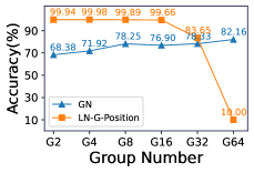
(a) Training.

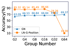
(b) Test.

Figure 6: Results of the variants of LN-G (GN and LN-G-Position) when using different group number. The experiments are conducted on CIFAR-10 dataset using ResNet without ReLU activation. We show (a) the training accuracy and (b) the test accuracy. In the x-axis, G2 refers to a group number of 2.

Investigation of LN-G.

Note that LN-G may have several variants for a convolutional input $\mX\in\mathbb{R}^{c\times h\times w}$, where $c$, $h$ and $w$ indicate the feature mappings’ channel, height and width dimensions respectively. Following the usage of LN on CNNs, LN-G should calculate the mean/variance along all the channel, height and width dimensions, which is equivalent to Group Normalization (GN) (Wu & He, 2018). Following the usage of LN on MLP$\&$Transformer, LN-G should calculate the mean/variance along only the channel dimension and use separate statistics over each position (a pair of height and width), and we refer to this method as LN-G-Position.

We investigate how the group number affects the performance of the variants of LN-G (GN and LN-G-Position). We vary the group number $g$ ranging in {2, 4, 8, 16, 32, 64}. We train a total of 200 epochs using SGD with a mini-batch size of 128, momentum of 0.9 and weight decay of 0.0001. The initial learning rate is set to 0.1, and divided by 5 at the 60th, 120th, and 160th epochs. The results are shown in Figure 6. We find that GN obtains slightly better performance as the group number increases. Note that this observation does not go against the experimental results of LN-G in amplifying the nonlinearity in Section 5.2 since the ‘effective samples’ used to calculate the normalization statistics in each group of GN is $\frac{h*w*c}{g}$. We observe that LN-G-Position works particularly well and obtains over $85\%$ test accuracy for multiple group number (Note that there is no ReLU activations.). We also find that LN-G-Position works particularly bad if group number is 64, because the samples used to calculate the normalization statistics in each group of LN-G-Position is $\frac{c}{g}=2$.

Table 1: Comparison of different normalization methods on CIFAR-10 using ResNet-NA (ResNet without ReLU activation).

Normalization methods	Train Acc(%)	Test Acc(%)
IN	10	10
BN	36.0	39.3
LN	59.5	62.85
GN	82.16	69.37
LN-G-Position	99.66	86.66

Comparison to other Normalization.

We also conduct experiments to train ResNet-NA by using other normalization methods, including the original Batch Normalization (BN) (Ioffe & Szegedy, 2015), Layer Normalization (LN) (Ba et al., 2016), Instance Normalization (IN) (Ulyanov et al., 2016). Besides, we also train ResNet-NA without normalization. We use the same setting up described in previous experiments. We find that ResNet-NA without normalization is very difficult to train and shows a random guess behavior. Similarly, ResNet-NA with IN is also very difficult to train. ResNet-NA with BN can be trained normally. However, the performance of the model is relatively low, with only $39.3\%$ test accuracy. ResNet-NA with LN obtains $62.85\%$ test accuracy, which is significantly better than BN. Furthermore, ResNet-NA with LN-G-Position obtains the best performance, e.g., a test accuracy of $86.66\%$ when using a group number 16 for LN-G-Position. We contribute it to the strong nonlinearity of LN-G-Position.

5.3.2 LN-G in Transformers

Transformer for Machine Translation.

We conduct experiments to apply LN-G on Transformer (Vaswani et al., 2017) (where LN is the default normalization) for machine translation tasks using fairseq-py (Ott et al., 2019). We evaluate the public IWSLT14 German-to-English (De-EN) dataset using BLEU (higher is better). We use the hyper-parameters recommended in fairseq-py (Ott et al., 2019) for Transformer and train over 50 epochs with five random seeds. The baseline LN has a BLEU score of $35.01\pm 0.10$. LN-G (replacing all the LNs with LN-G) has a BLEU score of $35.23\pm 0.07$.

ViT for Image Classification.

We conducted experiments by applying LN-G to Tiny-VIT (with the default normalization being LN). We performed classification tests on the test set of the CIFAR-10 dataset, with hyperparameter settings referencing (Steiner et al., 2021). The classification accuracy on the test dataset was $88.81\%$ for LN and $89.26\%$ for LN-G (replacing all the LNs with LN-G).

These preliminary results show the potentiality of LN-G used for neural architecture design in practice.

6 Related Work

Previous theoretical analyses on normalization are mainly focused on BN, the pioneer work in normalization for deep learning. One main argument is that BN can improve the conditioning of the optimization problem (Cai et al., 2019), either by avoiding the rank collapse of pre-activation matrices (Daneshmand et al., 2020) or by alleviating the pathological sharpness of the landscape (Santurkar et al., 2018; Karakida et al., 2019; Ghorbani et al., 2019; Lyu et al., 2022). The improved conditioning enables large learning rates (Bjorck et al., 2018), thus improving the generalization (Luo et al., 2019). Another argument is that BN is scale invariant (Ba et al., 2016), enabling it to adaptively adjust the learning rate (Arora et al., 2019; Cai et al., 2019; Zhang et al., 2019; Li & Arora, 2020), which stabilizes and further accelerates training. This scale invariant analyses also applies to LN (Ba et al., 2016; Lubana et al., 2021). Some work address to understanding LN empirically through experiments, showing that the learnable parameters in LN increases the risk of over-fitting (Xu et al., 2019).

Different from these work, we investigate a new theoretical direction for LN, regarding to its nonlinearity and representation capacity. We note that there are several work (Huang et al., 2021; Labatie et al., 2021) investigating the expressive power of normalization empirically by experiments. However, their experiments are conducted on networks with activation functions, while our work focuses on analyzing the representation capacity of a network without activation functions through theory and experiment.

7 Conclusion

We mathematically demonstrated that LN is a nonlinear transformation. We also theoretically showed the representation capacity of an LN-Net in correctly classifying samples with any label assignment. We demonstrated these results by finely designing algorithms, considering the geometric property of LN. We hope that our techniques will inspire the community to reconsider the analyses of the representation capacity of a network with normalization layer, though it suffers from great challenges (Huang et al., 2023).

Limitation and Future Work.

Our results in representation capacity for LN-Net is very loose currently, which is like the initial universal approximation theory in the arbitrary wide shallow neural network (Hornik et al., 1989). We believe it is interesting to extend our results along the direction as universal approximation theory is extended to the cases of arbitrary depth (Gripenberg, 2003), bounded depth and bounded width (Maiorov & Pinkus, 1999), and the question of minimal possible width (Park et al., 2020). Besides, the effectiveness of group mechanism for LN (i.e., LN-G) is only verified on small-scale networks and datasets, and more results on large-scale networks and datasets are required to support the practicality of LN-G.

Impact Statement

This paper presents work whose goal is to advance the field of Machine Learning. There are many potential social consequences of our work, none which feel must be specifically highlighted here.

Appendix A LSSR as a Linearly Separable Indicator

(a) XOR data.

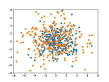
(b) Inseparable Gaussian data.

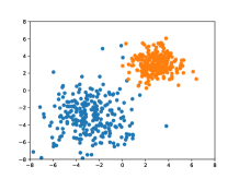
(c) Separable Gaussian data.

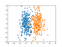
(d) Parallel Gaussian data.

Figure A1: We randomly sample $256$ points from each class in the four different distributions of data above. The detailed data is shown in Table A.

To show how SSR and LSSR evaluate the difficulty of separating the samples from different classes linearly, we give four different distributions of data in the figure above and their details in the table below.

Table I: Detailed data of Figure A1. In Figure 1(a), the random variance $X$ takes values $0$ and $1$ with probabilities $1/2$ each. In the other figures, the sign $N(\cdot,\cdot)$ denotes the Gaussian distribution.

Figure	Distribution of $X_{1}$	Distribution of $X_{2}$	SSR	LSSR
Figure 1(a)	$X_{1}=\mat$
X $&$ X_2 = X
1-X$&0.996$	0.9929
Figure 1(b)	$X_{1}\sim N\left($
0,4	0
0	4)	$X_{2}\sim N\left($
0,9	0
0		0.9929	0.9859
Figure 1(c)	$X_{1}\sim N\left($
-3,4	0
0	4)	$X_{2}\sim N\left($
3,1	0
0		0.2304	0.1312
Figure 1(d)	$X_{1}\sim N\left($
0,1	0
0	9)	$X_{2}\sim N\left($
0,1	0
0		0.7536	0.2157

According to Figure A1 and Table A, we have several conclusions below. In Figure 1(a) and Figure 1(b), the classes are hard to be linearly separated, whose SSR and LSSR are both near $1$. In Figure 1(c), the classes are easy to be linearly separated, whose SSR and LSSR are both near $0$. However, in Figure 1(d), the classes are easy to be linearly separated, but harder to be separated if focused on the Euclidean distance. As a result, its SSR is larger, but its LSSR is near $0$. We hence conclude that—LSSR is a better indicator than SSR in judging how two classes are linearly separable.

Appendix B Proofs of Proposition 2

Proposition 2.

Given $\mX_{1},\mX_{2}\in\R^{d\times m}$, we denote $\mM=\sum\limits_{c=1}^{2}\sum\limits_{i=1}^{m}(\rvx_{ci}-\bar{\rvx}_{c})(\rvx_{ci}-\bar{\rvx}_{c})^{\top}$, and $\mN=\sum\limits_{c=1}^{2}\sum\limits_{i=1}^{m}(\rvx_{ci}-\bar{\rvx})(\rvx_{ci}-\bar{\rvx})^{\top}$, where $\bar{\rvx}=(\bar{\rvx}_{1}+\bar{\rvx}_{2})/2$. Supposing that $\mN$ is reversible, we have

$$LSSR(\mX_{1},\mX_{2})=\lambda^{*},$$ (23)

and correspondingly,

$$LSSR(\mX_{1},\mX_{2})=SSR((\vu^{*})^{\top}\mX_{1},(\vu^{*})^{\top}\mX_{2}),$$ (24)

where $\lambda^{*}$ and $\vu^{*}$ are the minimum eigenvalue and corresponding eigenvector of $\mN^{-1}\mM$.

Since the definition of LSSR comes from a lower bound, we prove Proposition 2 from solving the optimization problem as follows.

$$(P_{LSSR})\begin{cases}\min\limits_{\varphi}\quad&LSSR(\mX_{1},\mX_{2})=SSR(\varphi(\mX_{1}),\varphi(\mX_{2})),\\ \text{s.t.}\quad&\varphi(\rvx)=\mW\rvx+\vb,\\ &\mW\in\R^{n\times d},\vb\in\R^{n},n\in\sN^{*},\\ &SS(\varphi(\mX_{1}),\varphi(\mX_{2}))\neq 0.\end{cases}$$ (25)

To solve this, we first propose four lemmas, and then use them to prove Proposition 2. Furthermore, we give the optimal $\mW$ as a corollary.

B.1 Required Lemmas for the Proof

Lemma 2.

The bias $\vb\in\R^{n}$ does not affect SSR, as well as LSSR.

Proof.

By the definition of SS, we obtain

$$SS(\varphi(\mX_{1})) =SS(\mW\mX_{1}+\vb\bm 1^{\top})$$ (26)

$$=\sum_{i=1}^{m}\left\|\mW\rvx_{1i}+\vb-\frac{1}{m}\sum_{i=1}^{m}(\mW\rvx_{1i}+\vb)\right\|^{2}$$

$$=\sum_{i=1}^{m}\left\|\mW\rvx_{1i}-\frac{1}{m}\sum_{i=1}^{m}\mW\rvx_{1i}\right\|^{2}$$

$$=\sum_{i=1}^{m}\left\|\mW\rvx_{1i}-\overline{\mW\rvx_{1}}\right\|^{2}$$

$$=SS(\mW\mX_{1}).$$

Similarly, we have

$$SS(\varphi(\mX_{2}))=SS(\mW\mX_{2}),$$ (27)

and

$$SS([\varphi(\mX_{1}),\varphi(\mX_{2})])=SS([\mW\mX_{1},\mW\mX_{2}]).$$ (28)

Since SSR is defined with SS, the conclusion also holds for SSR, namely

$$SSR(\varphi(\mX_{1}),\varphi(\mX_{2}))=SSR(\mW\mX_{1},\mW\mX_{2}),$$ (29)

where the bias $\vb$ is not included. ∎

Lemma 3.

Suppose the eigenvalue decomposition of $\mW^{\top}\mW$ as

$$\mW^{\top}\mW=\mU\Lambda\mU^{\top}=\sum_{i=1}^{d}\lambda_{i}\vu_{i}\vu_{i}^{\top},$$ (30)

where $\mU=[\vu_{1},\cdots,\vu_{d}]$ is an orthogonal matrix, and $\Lambda=diag\{\lambda_{1},\cdots,\lambda_{d}\}$ is a positive semi-definite and diagonal matrix. We consider to minimize $SSR(\mW\mX_{1},\mW\mX_{2})$ over $\Lambda$ with a fixed $\mU$, as:

$$\min_{\Lambda}SSR(\mW\mX_{1},\mW\mX_{2})=\min_{1\leq j\leq d}SSR(\vu_{j}^{\top}\mX_{1},\vu_{j}^{\top}\mX_{2}).$$ (31)

The optimal solution is that

$$\lambda_{j}\begin{cases}\geq 0,&j\in\arg\min\limits_{1\leq j\leq d}SSR(\vu_{j}^{\top}\mX_{1},\vu_{j}^{\top}\mX_{2}),\\ =0,&\text{otherwise},\end{cases}$$ (32)

for $j=1,\cdots,d$, and $\lambda_{1},\cdots,\lambda_{d}$ are not all zeros.

Proof.

By Lemma 2, we find that

$$LSSR(\mX_{1},\mX_{2})=\min_{\mW}SSR(\mW\mX_{1},\mW\mX_{2}).$$ (33)

Besides, we figure out that

$$SS(\mW\mX_{c})=\sum_{i=1}^{m}\left\|\mW\rvx_{ci}-\mW\bar{\rvx}_{c}\right\|_{2}^{2}=\sum_{i=1}^{m}(\rvx_{ci}-\bar{\rvx}_{c})^{\top}\mW^{\top}\mW(\rvx_{ci}-\bar{\rvx}_{c}),$$ (34)

where $\mX_{c}=\mX_{1},\mX_{2}$, or even $[\mX_{1},\mX_{2}]$.

Based on the eigenvalue decomposition, we obtain that

$$SS(\mW\mX_{1})= \sum_{i=1}^{m}(\rvx_{1i}-\bar{\rvx}_{1})^{\top}\mW^{\top}\mW(\rvx_{1i}-\bar{\rvx}_{1})$$ (35)

$$= \sum_{i=1}^{m}\sum_{j=1}^{d}\lambda_{j}(\rvx_{1i}-\bar{\rvx}_{1})^{\top}\vu_{j}\vu_{j}^{\top}(\rvx_{1i}-\bar{\rvx}_{1})$$

$$= \sum_{j=1}^{d}\lambda_{j}\sum_{i=1}^{m}(\vu_{j}^{\top}\rvx_{1i}-\vu_{j}^{\top}\bar{\rvx}_{1})^{2}$$

$$= \sum_{j=1}^{d}\lambda_{j}SS(\vu_{j}^{\top}\mX_{1}).$$

The term $SS(\vu_{j}^{\top}\mX_{1})$ can be regarded as that we put a linear transformation $\vu_{j}^{\top}$ on $\mX_{1}$, and then calculate its SS.

Similarly, we have that

$$SS(\mW\mX_{2})=\sum\limits_{j=1}^{d}\lambda_{j}SS(\vu_{j}^{\top}\mX_{2}),$$ (36)

and

$$SS([\mW\mX_{1},\mW\mX_{2}])=\sum\limits_{j=1}^{d}\lambda_{j}SS([\vu_{j}^{\top}\mX_{1},\vu_{j}^{\top}\mX_{2}]).$$ (37)

Therefore, we obtain

$$\begin{aligned} SSR(\mW\mX_{1},\mW\mX_{2})=\frac{\sum\limits_{j=1}^{d}\lambda_{j}[SS(\vu_{j}^{\top}\mX_{1})+SS(\vu_{j}^{\top}\mX_{2})]}{\sum\limits_{j=1}^{d}\lambda_{j}SS([\vu_{j}^{\top}\mX_{1},\vu_{j}^{\top}\mX_{2}])}\end{aligned}.$$ (38)

By the definition of $\mM$ and $\mN$ in Proposition 2, we obtain that

$$SS(\vu_{j}^{\top}\mX_{1})+SS(\vu_{j}^{\top}\mX_{2}) =\sum_{i=1}^{m}[(\vu_{j}^{\top}\rvx_{1i}-\vu_{j}^{\top}\bar{\rvx}_{1})^{2}+(\vu_{j}^{\top}\rvx_{2i}-\vu_{j}^{\top}\bar{\rvx}_{2})^{2}]$$ (39)

$$=\sum_{i=1}^{m}\vu_{j}^{\top}[(\rvx_{1i}-\bar{\rvx}_{1})(\rvx_{1i}-\bar{\rvx}_{1})^{\top}+(\rvx_{2i}-\bar{\rvx}_{2})(\rvx_{2i}-\bar{\rvx}_{2})^{\top}]\vu_{j}$$

$$=\vu_{j}^{\top}\mM\vu_{j},$$

and similarly, we have

$$SS([\vu_{j}^{\top}\mX_{1},\vu_{j}^{\top}\mX_{2}])=\vu_{j}^{\top}\mN\vu_{j}.$$ (40)

By the hypothesis in Definition 2, we figure out that $\lambda_{j}(j=1,\cdots,d)$ are not all zeros, otherwise $SS([\mW\mX_{1},\mW\mX_{2}])=0$. Besides, by the hypothesis in Proposition 2, $\mN$ is reversible. We point out that $\mN$ is also a positive semi-definite matrix.

Furthermore, $\mN$ is a positive definite matrix. When $\vu_{j}\neq\bm 0$, we find that

$$SS([\vu_{j}^{\top}\mX_{1},\vu_{j}^{\top}\mX_{2}])=\vu_{j}^{\top}\mN\vu_{j}>0.$$ (41)

Let $\eta_{j}=\lambda_{j}SS([\vu_{j}^{\top}\mX_{1},\vu_{j}^{\top}\mX_{2}])$, we thus have $\eta_{1}+\cdots+\eta_{d}>0$. We obtain

$$SSR(\mW\mX_{1},\mW\mX_{2})= \frac{1}{\eta_{1}+\cdots+\eta_{d}}\sum_{j=1}^{d}\frac{\eta_{j}[SS(\vu_{j}^{\top}\mX_{1})+SS(\vu_{j}^{\top}\mX_{2})]}{SS([\vu_{j}^{\top}\mX_{1},\vu_{j}^{\top}\mX_{2}])}$$ (42)

$$= \sum_{j=1}^{d}\frac{\eta_{j}}{\eta_{1}+\cdots+\eta_{d}}SSR(\vu_{j}^{\top}\mX_{1},\vu_{j}^{\top}\mX_{2})$$

$$\geq \sum_{j=1}^{d}\frac{\eta_{j}}{\eta_{1}+\cdots+\eta_{d}}\min_{1\leq k\leq d}SSR(\vu_{k}^{\top}\mX_{1},\vu_{k}^{\top}\mX_{2})$$

$$= \min_{1\leq k\leq d}SSR(\vu_{k}^{\top}\mX_{1},\vu_{k}^{\top}\mX_{2})$$

$$= \min_{1\leq j\leq d}SSR(\vu_{j}^{\top}\mX_{1},\vu_{j}^{\top}\mX_{2}).$$

We figure out that the equation holds, if and only if

$$\eta_{j}\begin{cases}\geq 0,&j\in\arg\min\limits_{1\leq j\leq d}SSR(\vu_{j}^{\top}\mX_{1},\vu_{j}^{\top}\mX_{2});\\ =0,&\text{otherwise}.\end{cases}$$ (43)

Here, $j=1,\cdots,d$, and $\eta_{1},\cdots,\eta_{d}$ are not all zeros.

Since $\lambda_{j}=\eta_{j}/SS([\vu_{j}^{\top}\mX_{1},\vu_{j}^{\top}\mX_{2}])$ and $SS([\vu_{j}^{\top}\mX_{1},\vu_{j}^{\top}\mX_{2}])>0$, we thus have

$$\lambda_{j}\begin{cases}\geq 0,&j\in\arg\min\limits_{1\leq j\leq d}SSR(\vu_{j}^{\top}\mX_{1},\vu_{j}^{\top}\mX_{2}),\\ =0,&\text{otherwise},\end{cases}$$ (44)

holds for $j=1,\cdots,d$, and $\lambda_{1},\cdots,\lambda_{d}$ are not all zeros. ∎

Lemma 4.

Given $\sD_{\vv}=\{\vv:\vv^{\top}\mN\vv=1\}$ and $\sD_{\vu}=\{\vu:\vu^{\top}\vu=1\}$ and the map $\psi:\sD_{\vv}\to\sD_{\vu}$, where $\vu=\psi(\vv)=\vv/(\vv^{\top}\vv)^{\frac{1}{2}}$, we have that $\psi$ is a bijection.

Proof.

For $\mN$ is a positive definite matrix , and $\vv^{\top}\mN\vv=1$, we have $\vv\neq\bm 0$. Given $\vu=\psi(\vv)$, we obtain

$$\vu^{\top}\vu=\vv^{\top}\vv/(\vv^{\top}\vv)=1,$$ (45)

for each $\vv$ in $\sD_{\vv}$.

Therefore, $\psi$ is a reflection from $\sD_{\vv}$ to $\sD_{\vu}$. Besides, we find that

$$\vu^{\top}\mN\vu=\vv^{\top}\mN\vv/(\vv^{\top}\vv)=1/(\vv^{\top}\vv).$$ (46)

By the definition of $\psi$, we hence have

$$\vu/(\vu^{\top}\mN\vu)^{\frac{1}{2}}=\psi(\vv)(\vv^{\top}\vv)^{\frac{1}{2}}=\vv.$$ (47)

Therefore, for each $\vu$, we obtain that

$$\vv=\psi^{-1}(\vu)=\vu/(\vu^{\top}\mN\vu)^{\frac{1}{2}},$$ (48)

namely we find $\psi^{-1}$ as the inverse mapping of $\psi$.

As a result, $\psi$ is a bijection. ∎

Lemma 5.

Let the optimization problem be

$$(P_{\vv})\begin{cases}\min\limits_{\vv}\quad&\displaystyle f(\vv)=\frac{\vv^{\top}\mM\vv}{\vv^{\top}\mN\vv},\\ s.t.\quad&\vv^{\top}\mN\vv=1,\end{cases}$$ (49)

where $\mM$ and $\mN$ are defined in Proposition 2. We have that the optimal value is the minimal eigenvalue of $\mN^{-1}\mM$, namely $\lambda^{*}$. And the optimal solution is the eigenvector which belongs to $\lambda^{*}$.

Proof.

To get the minimum, we use the Lagrange multiplier method:

$$L(\vv,\alpha)=\vv^{\top}\mM\vv-\alpha(\vv^{\top}\mN\vv-1).$$ (50)

We figure out that the KKT conditions are

$$\begin{cases}\displaystyle\frac{\partial L}{\partial\vv}=2\mM\vv-2\alpha\mN\vv=\bm 0,\\ \vv^{\top}\mN\vv-1=0.\end{cases}$$ (51)

We hence have $\mN^{-1}\mM\vv=\alpha\vv$, namely $\alpha$ is an eigenvalue of $\mN^{-1}\mM$, and $\vv$ is the corresponding eigenvector. Based above, we find that

$$\vv^{\top}\mM\vv=\vv^{\top}\mN\mN^{-1}\mM\vv=\vv^{\top}\mN(\alpha\vv)=\alpha.$$ (52)

Furthermore, the minimum of $L(\vv,\alpha)$ is the minimum $\alpha$, namely the minimum eigenvalue of $\mN^{-1}\mM$.

We hence have

$$LSSR(\mX_{1},\mX_{2})=\lambda_{min}(\mN^{-1}\mM)=\lambda^{*},$$ (53)

and the optimal solution is the eigenvector which belongs to $\lambda^{*}$. ∎

B.2 Proof of Proposition 2

Based on the four lemmas above, now we give the proof of Proposition 2.

Proof.

By Lemma 2 and Lemma 3, given $\mW^{\top}\mW=\mU\Lambda\mU^{\top}$, we have

$$LSSR(\mX_{1},\mX_{2}) =\min_{\mW}SSR(\mW\mX_{1},\mW\mX_{2})$$ (54)

$$=\min_{\mU,\Lambda}SSR(\mW\mX_{1},\mW\mX_{2})$$

$$=\min_{\mU}\min_{\Lambda}SSR(\mW\mX_{1},\mW\mX_{2})$$

$$=\min_{\mU}\min\limits_{1\leq j\leq d}SSR(\vu_{j}^{\top}\mX_{1},\vu_{j}^{\top}\mX_{2}).$$

According to 39 and 40, we define the function $f(\vu)=SSR(\vu^{\top}\mX_{1},\vu^{\top}\mX_{2})$, namely

$$f(\vu)=\frac{\vu^{\top}\mM\vu}{\vu^{\top}\mN\vu}.$$ (55)

By 54, there is some $\mU$, and $j^{*}=\arg\min\limits_{1\leq j\leq d}SSR(\vu_{j}^{\top}\mX_{1},\vu_{j}^{\top}\mX_{2})$, such that

$$LSSR(\mX_{1},\mX_{2})=\min\limits_{1\leq j\leq d}SSR(\vu_{j}^{\top}\mX_{1},\vu_{j}^{\top}\mX_{2})=f(\vu_{j^{*}}).$$ (56)

Consider the optimization problem

$$(P_{\vu})\begin{cases}\min\limits_{\vu}\quad&f(\vu)=\displaystyle\frac{\vu^{\top}\mM\vu}{\vu^{\top}\mN\vu},\\ s.t.\quad&\vu^{\top}\vu=1.\end{cases}$$ (57)

We denote one of the optimal solutions as $\bar{\vu}$. Obviously, $\vu_{j^{*}}$ is one of the feasible solutions above, we thus have

$$LSSR(\mX_{1},\mX_{2})=f(\vu_{j^{*}})\geq f(\bar{\vu}).$$ (58)

We remind that $\lambda^{*}$ and $\vu^{*}$ are the minimum eigenvalue and corresponding eigenvector of $\mN^{-1}\mM$. On one hand, let $\vu_{0}=\vu^{*}/\|\vu^{*}\|_{2}$ and $\vv_{0}=\psi^{-1}(\vu_{0})$ ($\psi$ is defined the same as that in Lemma 4), namely $\vv_{0}=\vu_{0}/(\vu_{0}^{\top}\mN\vu_{0})^{\frac{1}{2}}$. We first point out that for $k\neq 0$, we have

$$f(k\vu) =\frac{(k\vu)^{\top}\mM(k\vu)}{(k\vu)^{\top}\mN(k\vu)}$$ (59)

$$=\frac{\vu^{\top}\mM\vu}{\vu^{\top}\mN\vu}$$

$$=f(\vu).$$

Since $1/||\vu^{*}||_{2}\neq 0$ and $1/(\vu_{0}^{\top}\mN\vu_{0})^{\frac{1}{2}}\neq 0$, we obtain

$$f(\vv_{0})=f(\vu_{0}) =f(\vu^{*})$$ (60)

$$=\frac{(\vu^{*})^{\top}\mM(\vu^{*})}{(\vu^{*})^{\top}\mN(\vu^{*})}$$

$$=\frac{(\vu^{*})^{\top}\mN\mN^{-1}\mM(\vu^{*})}{(\vu^{*})^{\top}\mN(\vu^{*})}$$

$$=\frac{(\vu^{*})^{\top}\mN(\lambda^{*}\vu^{*})}{(\vu^{*})^{\top}\mN(\vu^{*})}$$

$$=\lambda^{*},$$

where $\lambda^{*}$ is the minimal eigenvalue of $\mN^{-1}\mM$, as shown in Proposition 2.

Therefore, by Lemma 5, $\vv_{0}$ is the optimal solution of $(P_{\vv})$. Furthermore, by Lemma 4, since $\psi$ is a bijection between $\sD_{\vv}$ and $\sD_{\vu}$ and $f(\psi(\vv))=f(\vv)$, we have that $\vu_{0}=\psi(\vv_{0})$ is also the optimal solution of $(P_{\vu})$. We hence have $f(\vu^{*})=f(\vu_{0})=f(\bar{\vu})$. By 58, we obtain

$$LSSR(\mX_{1},\mX_{2})\geq f(\bar{\vu})=f(\vu^{*})=SSR((\vu^{*})^{\top}\mX_{1},(\vu^{*})^{\top}\mX_{2}).$$ (61)

On the other hand, the definition of LSSR denotes the lower bound of SSR, we hence have

$$LSSR(\mX_{1},\mX_{2})\leq SSR((\vu^{*})^{\top}\mX_{1},(\vu^{*})^{\top}\mX_{2}).$$ (62)

By 60, 61 and 62, we obtain

$$LSSR(\mX_{1},\mX_{2})=SSR((\vu^{*})^{\top}\mX_{1},(\vu^{*})^{\top}\mX_{2})=\lambda^{*}.$$ (63)

∎

B.3 Corollaries of Proposition 2

Suppose $\lambda^{*}$ is the minimal eigenvalue of $\mN^{-1}\mM$, and $\vu^{*}$ is its unique linearly independent eigenvector, we give the result in Corollary 4. If $\lambda^{*}$ has more than one linearly independent eigenvectors, we give the result in Corollary 5.

Corollary 4.

Suppose $\lambda^{*}$ is the minimal eigenvalue of $\mN^{-1}\mM$, and $\vu^{*}$ is its unique linearly independent eigenvector, we have that the optimal $\mW$ satisfies that

$$\mW^{\top}\mW=C\vu^{*}(\vu^{*})^{\top},C>0.$$ (64)

Proof.

By Lemma 2, we can only consider the eigenvalues and eigenvectors of $\mW^{\top}\mW$. By 30, $\vu_{j}$ will affect $\mW^{\top}\mW$ only when the corresponding eigenvalue $\lambda_{j}\neq 0$. Furthermore, by Lemma 3, when $\lambda_{j}\neq 0$, we figure out that

$$j\in\arg\min\limits_{1\leq j\leq d}SSR(\vu_{j}^{\top}\mX_{1},\vu_{j}^{\top}\mX_{2}).$$ (65)

Since $\vu_{j}$ is a unit vector, it must be one of the optimal solutions of $(P_{\vu})$. We hence have $f(\vu_{j})=\lambda^{*}$. By 59 and Lemma 4, we have

$$f(\psi^{-1}(\vu_{j}))=f(\vu_{j})=\lambda^{*},$$ (66)

and $\psi^{-1}(\vu_{j})$ is one of the optimal solutions of $(P_{\vv})$. By Lemma 5, we have that $\psi^{-1}(\vu_{j})$ must satisfy the KKT conditions in 51, namely

$$\mN^{-1}\mM\psi^{-1}(\vu_{j})=\lambda^{*}\psi^{-1}(\vu_{j}).$$ (67)

Therefore, $\psi^{-1}(\vu_{j})$ is the minimal eigenvector of $\mM^{-1}\mN$. For $\psi^{-1}(\vu_{j})=\vu_{j}/(\vu_{j}^{\top}\mN\vu_{j})^{\frac{1}{2}}$, we obtain $\vu_{j}$ is also the eigenvector of $\lambda^{*}$. For $\vu^{*}$ is the unique linearly independent eigenvector of $\lambda^{*}$, we figure out that

$$\vu_{j}=\alpha_{j}\vu^{*},\alpha_{j}\neq 0.$$ (68)

To be reminded, 68 only holds when $\lambda_{j}\neq 0$. Therefore, we have

$$\mW^{\top}\mW =\sum_{j=1}^{d}\lambda_{j}\vu_{j}\vu_{j}^{\top}$$ (69)

$$=\sum_{\lambda_{j}\neq 0}\lambda_{j}\alpha_{j}^{2}\vu^{*}(\vu^{*})^{\top}$$

$$=C\vu^{*}(\vu^{*})^{\top},$$

where $C=\sum\limits_{\lambda_{j}\neq 0}\lambda_{j}\alpha_{j}^{2}$.

By Lemma 3, we have $\lambda_{1},\cdots,\lambda_{j}\geq 0$ are not all zeros. Besides, we figure out that $\alpha_{j}$ can be any non-zero real number. We thus have $C$ can be any non-zero real number, to demonstrate $\mW^{\top}\mW$. ∎

Corollary 5.

Suppose that the minimal eigenvalue of $\mN^{-1}\mM$, namely $\lambda^{*}$, has $k$ linearly independent eigenvectors $\vv_{1},\vv_{2},\cdots,\vv_{k}$. We denote $\mV=[\vv_{1},\cdots,\vv_{k}]$, then we have that the optimal $\mW$ satisfies that

$$\mW^{\top}\mW=\mV\mC\mV^{\top},$$ (70)

where $\mC$ is a $k$-order semi-positive definite and non-zero matrix.

Proof.

Suppose $\lambda_{j}$ is an eigenvalue of $\mW^{\top}\mW$, and its eigenvector is $\vu_{j}$. We can identify that $j\in\arg\min\limits_{1\leq j\leq d}SSR(\vu_{j}^{\top}\mX_{1},\vu_{j}^{\top}\mX_{2})$, if $\lambda_{j}\neq 0$. Similarly to the proof of Corollary 4, $\vu_{j}$ must be an eigenvector of $\mN^{-1}\mM$, and the corresponding eigenvalue is $\lambda^{*}$. Accordingly, $\vu_{j}$ is a linear combination of all the linearly independent eigenvectors of $\lambda^{*}$, namely

$$\vu_{j}=\alpha_{j1}\vv_{1}+\alpha_{j2}\vv_{2}+\cdots+\alpha_{jk}\vv_{k}=\mV\bm\alpha_{j}$$ (71)

where $\bm\alpha_{j}=[\alpha_{j1},\cdots,\alpha_{jk}]^{\top}$, and $\bm\alpha_{j}\neq\bm 0$.

We remind that 71 only holds when $\lambda_{j}\neq 0$. We thus have

$$\mW^{\top}\mW =\sum_{j=1}^{d}\lambda_{j}\vu_{j}\vu_{j}^{\top}$$ (72)

$$=\sum_{\lambda_{j}>0}\lambda_{j}\vu_{j}\vu_{j}^{\top}$$

$$=\sum_{\lambda_{j}>0}\lambda_{j}(\mV\bm\alpha_{j})(\mV\bm\alpha_{j})^{\top}$$

$$=\mV\left(\sum_{\lambda_{j}>0}\lambda_{j}\bm\alpha_{j}\bm\alpha_{j}^{\top}\right)\mV^{\top}$$

$$=\mV\mC\mV^{\top},$$

where $\mC=\sum\limits_{\lambda_{j}>0}\lambda_{j}\bm\alpha_{j}\bm\alpha_{j}^{\top}$.

By Lemma 3, we have $\lambda_{1},\cdots,\lambda_{j}\geq 0$ are not all zeros. Besides, we figure out that $\bm\alpha_{j}$ can be any non-zero vector. We thus have $\mC$ is any $k$-order semi-positive definite and non-zero matrix, to demonstrate $\mW^{\top}\mW$. ∎

Appendix C Proof Related to Breaking LSSR

In this section, we prove Theorem 1 from the perspective of Taylor’s expansion.

We have defined $f_{SSR}(t)$ as

$$f_{SSR}(t)=\begin{cases}LSSR(\mX_{1},\mX_{2}),&t=0,\\ SSR(\bar{\psi}(t;\mX_{1}),\bar{\psi}(t;\mX_{2})),&t\neq 0,\end{cases}$$ (73)

where $\bar{\psi}(t;\rvx_{ci})=\bm 1^{\top}\bar{\varphi}(t;\rvx_{ci})/\|\bar{\varphi}(t;\rvx_{ci})\|_{2}$, $\bar{\varphi}(t;\rvx_{ci})=[(\vu^{*})^{\top}\rvx_{ci}t,1]^{\top}$ and $t\in\R$. We remind Theorem 1 as below.

Theorem 1.

Let $\psi=\varphi_{1}\circ LN(\cdot)\circ\varphi_{2}$, performing over the input $\mX_{1},\mX_{2}\in\R^{d\times m}$. If $f_{SSR}^{\prime}(0)\neq 0$ , we can always find suitable linear functions $\varphi_{1}$ and $\varphi_{2}$, such that

$$SSR(\psi(\mX_{1}),\psi(\mX_{2}))<LSSR(\mX_{1},\mX_{2}).$$ (74)

We prove Lemma 1 and show three extra lemmas before the formal proof of Theorem 1.

C.1 Proof of Lemma 1

Lemma 1.

Denote $LN(\cdot)$ as the LN operation in $\R^{d}(d\geq 3)$, and $SP(\cdot)$ as the SP operation in $\R^{d-1}$. We can find some linear transformations $\hat{\varphi}_{1}$ and $\hat{\varphi}_{2}$, such that

$$SP(\cdot)=\hat{\varphi}_{1}\circ LN(\cdot)\circ\hat{\varphi}_{2}.$$ (75)

We denote that $SP(\cdot)$ is defined on $\R^{d-1}$, as

$$SP(\rvx)=\rvx/\|\rvx\|_{2}.$$ (76)

While $LN(\cdot)$ is defined on $\R^{d}$, where

$$LN(\rvx)=\sqrt{d}\ (\rvx-\frac{1}{d}\bm 1\bm 1^{\top}\rvx)/\|\rvx-\frac{1}{d}\bm 1\bm 1^{\top}\rvx\|_{2}.$$ (77)

Before the proof of Lemma 1, we propose Lemma 6 as follows.

Lemma 6.

There is some orthogonal matrix $\mQ\in\R^{d\times d}$, such that

0∈{

∈d:

References

- Alayrac et al. (2022) Alayrac, J.-B., Donahue, J., Luc, P., Miech, A., Barr, I., Hasson, Y., Lenc, K., Mensch, A., Millican, K., Reynolds, M., et al. Flamingo: a visual language model for few-shot learning. In NeurIPS, 2022.
- Arora et al. (2019) Arora, S., Li, Z., and Lyu, K. Theoretical analysis of auto rate-tuning by batch normalization. In ICLR, 2019.
- Ba et al. (2016) Ba, J. L., Kiros, J. R., and Hinton, G. E. Layer normalization, 2016.
- Bartlett et al. (1998) Bartlett, P., Maiorov, V., and Meir, R. Almost linear vc dimension bounds for piecewise polynomial networks. In NeurIPS, 1998.
- Bjorck et al. (2018) Bjorck, N., Gomes, C. P., Selman, B., and Weinberger, K. Q. Understanding batch normalization. In NeurIPS, 2018.
- Brown et al. (2020) Brown, T., Mann, B., Ryder, N., Subbiah, M., Kaplan, J. D., Dhariwal, P., Neelakantan, A., Shyam, P., Sastry, G., Askell, A., Agarwal, S., Herbert-Voss, A., Krueger, G., Henighan, T., Child, R., Ramesh, A., Ziegler, D., Wu, J., Winter, C., Hesse, C., Chen, M., Sigler, E., Litwin, M., Gray, S., Chess, B., Clark, J., Berner, C., McCandlish, S., Radford, A., Sutskever, I., and Amodei, D. Language models are few-shot learners. In NeurIPS, 2020.
- Cai et al. (2019) Cai, Y., Li, Q., and Shen, Z. A quantitative analysis of the effect of batch normalization on gradient descent. In ICML, 2019.
- Carion et al. (2020) Carion, N., Massa, F., Synnaeve, G., Usunier, N., Kirillov, A., and Zagoruyko, S. End-to-end object detection with transformers. In ECCV, 2020.
- Cheng et al. (2022) Cheng, B., Misra, I., Schwing, A. G., Kirillov, A., and Girdhar, R. Masked-attention mask transformer for universal image segmentation. In CVPR, 2022.
- Dai et al. (2019) Dai, Z., Yang, Z., Yang, Y., Carbonell, J., Le, Q., and Salakhutdinov, R. Transformer-XL: Attentive language models beyond a fixed-length context. In ACL, 2019.
- Daneshmand et al. (2020) Daneshmand, H., Kohler, J. M., Bach, F. R., Hofmann, T., and Lucchi, A. Batch normalization provably avoids ranks collapse for randomly initialised deep networks. In NeurIPS, 2020.
- Devlin et al. (2019) Devlin, J., Chang, M.-W., Lee, K., and Toutanova, K. BERT: Pre-training of deep bidirectional transformers for language understanding. In ACL, 2019.
- Dosovitskiy et al. (2021) Dosovitskiy, A., Beyer, L., Kolesnikov, A., Weissenborn, D., Zhai, X., Unterthiner, T., Dehghani, M., Minderer, M., Heigold, G., Gelly, S., Uszkoreit, J., and Houlsby, N. An image is worth 16x16 words: Transformers for image recognition at scale. In ICLR, 2021.
- Fisher (1970) Fisher, R. A. Statistical methods for research workers. In Breakthroughs in statistics: Methodology and distribution, pp. 66–70. Springer, 1970.
- Ghorbani et al. (2019) Ghorbani, B., Krishnan, S., and Xiao, Y. An investigation into neural net optimization via hessian eigenvalue density. In ICML, 2019.
- Gripenberg (2003) Gripenberg, G. Approximation by neural networks with a bounded number of nodes at each level. Journal of approximation theory, 122(2):260–266, 2003.
- He et al. (2016) He, K., Zhang, X., Ren, S., and Sun, J. Deep residual learning for image recognition. In CVPR, 2016.
- Hoffer et al. (2018) Hoffer, E., Banner, R., Golan, I., and Soudry, D. Norm matters: efficient and accurate normalization schemes in deep networks. In NeurIPS, 2018.
- Hornik et al. (1989) Hornik, K., Stinchcombe, M., and White, H. Multilayer feedforward networks are universal approximators. Neural Networks, 2(5):359–366, 1989.
- Huang et al. (2021) Huang, L., Zhou, Y., Liu, L., Zhu, F., and Shao, L. Group whitening: Balancing learning efficiency and representational capacity. In CVPR, 2021.
- Huang et al. (2023) Huang, L., Qin, J., Zhou, Y., Zhu, F., Liu, L., and Shao, L. Normalization techniques in training dnns: Methodology, analysis and application. IEEE Transactions on Pattern Analysis and Machine Intelligence, 2023.
- Ioffe & Szegedy (2015) Ioffe, S. and Szegedy, C. Batch normalization: Accelerating deep network training by reducing internal covariate shift. In ICML, 2015.
- Karakida et al. (2019) Karakida, R., Akaho, S., and Amari, S.-i. The normalization method for alleviating pathological sharpness in wide neural networks. In NeurIPS, 2019.
- Kirillov et al. (2023) Kirillov, A., Mintun, E., Ravi, N., Mao, H., Rolland, C., Gustafson, L., Xiao, T., Whitehead, S., Berg, A. C., Lo, W.-Y., Dollar, P., and Girshick, R. Segment anything. In ICCV, 2023.
- Labatie et al. (2021) Labatie, A., Masters, D., Eaton-Rosen, Z., and Luschi, C. Proxy-normalizing activations to match batch normalization while removing batch dependence. In NeurIPS, 2021.
- Li & Arora (2020) Li, Z. and Arora, S. An exponential learning rate schedule for batch normalized networks. In ICLR, 2020.
- Lubana et al. (2021) Lubana, E. S., Dick, R., and Tanaka, H. Beyond batchnorm: towards a unified understanding of normalization in deep learning. In NeurIPS, 2021.
- Luo et al. (2019) Luo, P., Wang, X., Shao, W., and Peng, Z. Towards understanding regularization in batch normalization. In ICLR, 2019.
- Lyu et al. (2022) Lyu, K., Li, Z., and Arora, S. Understanding the generalization benefit of normalization layers: Sharpness reduction. In NeurIPS, 2022.
- Maiorov & Pinkus (1999) Maiorov, V. and Pinkus, A. Lower bounds for approximation by mlp neural networks. Neurocomputing, 25(1-3):81–91, 1999.
- Ott et al. (2019) Ott, M., Edunov, S., Baevski, A., Fan, A., Gross, S., Ng, N., Grangier, D., and Auli, M. fairseq: A fast, extensible toolkit for sequence modeling. In ACL, 2019.
- Park et al. (2020) Park, S., Yun, C., Lee, J., and Shin, J. Minimum width for universal approximation. arXiv preprint arXiv:2006.08859, 2020.
- Radford et al. (2021) Radford, A., Narasimhan, K., Salimans, T., Sutskever, I., et al. Improving language understanding by generative pre-training. 2021.
- Raffel et al. (2020) Raffel, C., Shazeer, N., Roberts, A., Lee, K., Narang, S., Matena, M., Zhou, Y., Li, W., and Liu, P. J. Exploring the limits of transfer learning with a unified text-to-text transformer. J. Mach. Learn. Res., 21(1), jan 2020.
- Santurkar et al. (2018) Santurkar, S., Tsipras, D., Ilyas, A., and Madry, A. How does batch normalization help optimization? In NeurIPS, 2018.
- Steiner et al. (2021) Steiner, A., Kolesnikov, A., Zhai, X., Wightman, R., Uszkoreit, J., and Beyer, L. How to train your vit? data, augmentation, and regularization in vision transformers. arXiv preprint arXiv:2106.10270, 2021.
- Ulyanov et al. (2016) Ulyanov, D., Vedaldi, A., and Lempitsky, V. S. Instance normalization: The missing ingredient for fast stylization. arXiv preprint arXiv:1607.08022, 2016.
- Vaswani et al. (2017) Vaswani, A., Shazeer, N., Parmar, N., Uszkoreit, J., Jones, L., Gomez, A. N., Kaiser, L. u., and Polosukhin, I. Attention is all you need. In NeurIPS, 2017.
- Wu & He (2018) Wu, Y. and He, K. Group normalization. In ECCV, 2018.
- Xiong et al. (2020) Xiong, R., Yang, Y., He, D., Zheng, K., Zheng, S., Xing, C., Zhang, H., Lan, Y., Wang, L., and Liu, T.-Y. On layer normalization in the transformer architecture. In ICML, 2020.
- Xu et al. (2019) Xu, J., Sun, X., Zhang, Z., Zhao, G., and Lin, J. Understanding and improving layer normalization. In NeurIPS, 2019.
- Zhang & Sennrich (2019) Zhang, B. and Sennrich, R. Root mean square layer normalization. In NeurIPS, 2019.
- Zhang et al. (2017) Zhang, C., Bengio, S., Hardt, M., Recht, B., and Vinyals, O. Understanding deep learning requires rethinking generalization. In ICLR, 2017.
- Zhang et al. (2019) Zhang, G., Wang, C., Xu, B., and Grosse, R. B. Three mechanisms of weight decay regularization. In ICLR, 2019.