1.2pt \AtAppendix \AtAppendix \AtAppendix \AtAppendix \AtAppendix \AtAppendix
Equivariant Machine Learning on Graphs with
Nonlinear Spectral Filters
Abstract
Equivariant machine learning is an approach for designing deep learning models that respect the symmetries of the problem, with the aim of reducing model complexity and improving generalization. In this paper, we focus on an extension of shift equivariance, which is the basis of convolution networks on images, to general graphs. Unlike images, graphs do not have a natural notion of domain translation. Therefore, we consider the graph functional shifts as the symmetry group: the unitary operators that commute with the graph shift operator. Notably, such symmetries operate in the signal space rather than directly in the spatial space. We remark that each linear filter layer of a standard spectral graph neural network (GNN) commutes with graph functional shifts, but the activation function breaks this symmetry. Instead, we propose nonlinear spectral filters (NLSFs) that are fully equivariant to graph functional shifts and show that they have universal approximation properties. The proposed NLSFs are based on a new form of spectral domain that is transferable between graphs. We demonstrate the superior performance of NLSFs over existing spectral GNNs in node and graph classification benchmarks.
1 Introduction
In many fields, such as chemistry [Gilmer et al., 2017], biology [Gaudelet et al., 2021, Barabasi and Oltvai, 2004], social science [Borgatti et al., 2009], and computer graphics [Wang et al., 2019], data can be described by graphs. In recent years, there has been a tremendous interest in the development of machine learning models for graph-structured data [Wu et al., 2020, Bronstein et al., 2017]. This young field, often called graph machine learning (graph-ML) or graph representation learning, has made significant contributions to the applied sciences, e.g., in protein folding, molecular design, and drug discovery [Jumper et al., 2021, Atz et al., 2021, Méndez-Lucio et al., 2021, Stokes et al., 2020], and has impacted the industry with applications in social media, recommendation systems, traffic prediction, computer graphics, and natural language processing, among others.
Geometric Deep Learning (GDL) [Bronstein et al., 2017] is a design philosophy for machine learning models where the model is constructed to inherently respect symmetries present in the data, aiming to reduce model complexity and enhance generalization. By incorporating knowledge of these symmetries into the model, it avoids the need to expend parameters and data to learn them. This inherent respect for symmetries is automatically generalized to test data, thereby improving generalization [Bietti et al., 2021, Petrache and Trivedi, 2024, Elesedy and Zaidi, 2021]. For instance, convolutional neural networks (CNNs) respect the translation symmetries of 2D images, with weight sharing due to these symmetries contributing significantly to their success [Krizhevsky et al., 2012]. Respecting node re-indexing in a scalable manner revolutionized machine learning on graphs [Bronstein et al., 2017, 2021] and has placed GNNs as a main general-purpose tool for processing graph-structured data. Moreover, within GNNs, respecting the 3D Euclidean symmetries of the laws of physics (rotations, reflections, and translations) led to state-of-the-art performance in molecule processing [Duval et al., 2024].
Our Contribution. In this paper, we focus on GDL for graph-ML. We consider extensions of shift symmetries from images to general graphs. Since graphs do not have a natural notion of domain translation, as opposed to images, we propose considering functional translations instead. We model the group of translations on graphs as the group of all unitary operators on signals that commute with the graph shift operator. Such unitary operators are called graph functional shifts. Note that each linear filter layer of a standard spectral GNN commutes with graph functional shifts, but the activation function breaks this symmetry. Instead, we propose non-linear spectral filters (NLSFs) that are fully equivariant to graph functional shifts and have universal approximation properties.
In Sec. 3, we introduce our NLSFs based on new notions of analysis and synthesis that map signals between their node-space representations and spectral representations. Our transforms are related to standard graph Fourier and inverse Fourier transforms but differ from them in one important aspect. One key property of our analysis transform is that it is independent of a specific choice of Laplacian eigenvectors. Hence, our spectral representations are transferable between graphs. In comparison, standard graph Fourier transforms are based on an arbitrary choice of eigenvectors, and therefore, the standard frequency domain is not transferable. To achieve transferability, standard graph Fourier methods resort to linear filter operations based on functional calculus. Since we do not have this limitation, we can operate on the frequency coefficients with arbitrary nonlinear functions such as multilayer perceptrons. In Sec. 4, we present theoretical results of our NLSFs, including the universal approximation and expressivity properties. In Sec. 5, we demonstrate the efficacy of our NLSFs in node and graph classification benchmarks, where our method outperforms existing spectral GNNs.
2 Background
Notation. For , we denote . We denote matrices by boldface uppercase letter , vectors (assumed to be columns) by lowercase boldface , and the entries of matrices and vectors are denoted with the same letter in lower case, e.g., . Let be an undirected graph with a node set , an edge set , an adjacency matrix representing the edge weights, and a node feature matrix containing -dimensional node attributes. Let be the diagonal degree matrix of , where the diagonal element is the degree of node . Denote by any normal graph shift operator (GSO). For example, could be the combinatorial graph Laplacian or the normalized graph Laplacian given by and , respectively. Let be the eigendecomposition of , where is the eigenvector matrix and is the diagonal matrix with eigenvalues ordered by . An eigenspace is the span of all eigenvectors corresponding to the same eigenvalue. Let denote the projection upon the -th eigenspace of in increasing order of . We denote the Euclidean norm by . We define the channel-wise signal norm of a matrix as the vector , where is the -th column on . We abbreviate multilayer perceptrons by MLP.
2.1 Linear Graph Signal Processing
Spectral GNNs define convolution operators on graphs via the spectral domain. Given a self-adjoint graph shift operator (GSO) , e.g., a graph Laplacian, the Fourier modes of the graph are defined to be the eigenvectors of and the eigenvalues are the frequencies. A spectral filter is defined to directly satisfy the “convolution theorem” [Bracewell and Kahn, 1966] for graphs. Namely, given a signal and a function , the operator defined by
| (1) |
is called a filter. Here, is the number of output channels. Spectral GNNs, e.g., [Defferrard et al., 2016b, Kipf and Welling, 2016, Levie et al., 2018, Bianchi et al., 2021], are graph convolutional networks where convolutions are via Eq. (1), with a trainable function at each layer, and a nonlinear activation function.
2.2 Equivariant GNNs
Equivariance describes the ability of functions to respect symmetries. It is expressed as , where is an action of a symmetry group on the domain of . GNNs [Scarselli et al., 2008, Bruna et al., 2013], including spectral GNNs [Defferrard et al., 2016a, Kipf and Welling, 2016] and subgraph GNNs [Frasca et al., 2022, Bevilacqua et al., 2022], are inherently permutation equivariant w.r.t. the ordering of nodes. This means that the network’s operations are unaffected by the specific arrangement of nodes, a property stemming from passive symmetries [Villar et al., 2023] where transformations are applied to both the graph signals and the graph domain. This permutation equivariance is often compared to the translation equivariance in CNNs [LeCun et al., 1995, 2010], which involves active symmetries [Huang et al., 2024]. The key difference between the two symmetries lies in the domain: while CNNs operate on a fixed domain with signals transforming within it, graphs lack a natural notion of domain translation. To address this, we consider graph functional shifts as the symmetry group, defined by unitary operators that commute with the graph shift operator. This perspective allows for our NLSFs to be interpreted as an extension of active symmetry within the graph context, bridging the gap between the passive and active symmetries inherent to GNNs and CNNs, respectively.
3 Nonlinear Spectral Graph Filters
In this section, we present new concepts of analysis and synthesis under which the spectral domain is transferrable between graphs. Following these concepts, we introduce new GNNs that are equivariant to functional symmetries – symmetries of the Hilbert space of signals rather than symmetries in the domain of definition of the signal [Lim et al., 2024].
3.1 Translation Equivariance of CNNs and GNNs
For motivation, we start with the grid graph with node set and circular adjacency , we define the translation operator by as
Note that any is a unitary operator that commutes with the grid Laplacian , i.e., , and therefore it belongs to the group of all unitary operators that commute with the grid Laplacian . In fact, the space of isotropic convolution operators (with 90o rotation and reflection symmetric filters) can be seen as the space of all normal operators111The operator is normal iff . Equivalently, iff has an orthogonal eigendecomposition. that commute with unitary operators from [Cohen and Welling, 2016]. Applying a non-linearity after the convolution retains this equivariance, and hence, we can build multi-layer CNNs that commute with . By the universal approximation theorem [Cybenko, 1989, Funahashi, 1989, Leshno et al., 1993], this allows us to approximate any continuous function that commutes with .
Note that such translation equivariance cannot be extended to general graphs. Achieving equivariance to graph functional shifts through linear spectral convolutional layers is straightforward, since these layers commute with the space of all unitary operators that commute with . However, introducing non-linearity breaks the symmetry. That is, there exists such that
This means that multi-layer spectral GNNs do not commute with , and are hence not appropriate as approximators of general continuous functions that commute with . Instead, we propose in this paper a multi-layer GNN that is fully equivariant to , which we show to be universal: it can approximate any continuous graph-signal function (w.r.t. some metric) commuting with .
3.2 Graph Functional Symmetries and Their Relaxations
We define the symmetry group of graph functional shifts as follows.
Definition 3.1 (Graph Functional Shifts).
The space of graph functional shifts is the unitary subgroup , where a unitary matrix is in iff it commutes with the GSO , namely, .
It is important to note that functional shifts, in general, are not induced from node permutations. Instead, functional shifts are related to the notion of functional maps [Ovsjanikov et al., 2012] used in shape correspondence.
A fundamental challenge with the symmetry group in Def. 3.1 is its lack of transferability between different graphs. Hence, we propose to relax this symmetry group. Let be the indicator functions of the intervals , which constitute a partition of the frequency band . The operators , interpreted via functional calculus Eq. (1), are projections of the signal space upon band-limited signals. Namely, . In our work, we consider filters that are supported on the dyadic sub-bands , where is the decay rate. See Fig. 3 in App. C for an illustrated example. Note that for , the sub-band falls in . The total band is .
Definition 3.2 (Relaxed Functional Shifts).
The space of relaxed functional shifts with respect to the filter bank (of indicators) is the unitary subgroup , where a unitary matrix is in iff it commutes with for all , namely, .
Similarly, we can relax functional shifts by restricting to the leading eigenspaces.
Definition 3.3 (Leading Functional Shifts).
The space of leading functional shifts is the unitary subgroup , where a unitary is in iff it commutes with the eigenspace projections .
3.3 Analysis and Synthesis
We use the terminology of analysis and synthesis, as in signal processing [Mallat, 1989], to describe transformations of signals between their graph and spectral representations. Here, we consider two settings: the eigenspace projections case and the filter bank (of indicators) case.
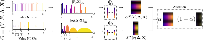
Spectral Index Case. We first define the analysis and synthesis using the spectral index by
| (2) |
respectively, where in synthesis, the product and division are element-wise. Here, are the spectral coefficients to be synthesized, and and are parameters that promote stability. The term index stems from the fact that eigenvalues are treated according to their index when defining the projections . Note that the synthesis here differs from classic signal processing as it depends on a given signal on the graph. When treating and as fixed, this synthesis operation is denoted by . We similarly denote .
Filter Bank Case. We also consider and define the analysis and synthesis in the filter bank by
| (3) |
respectively, where in synthesis, the product and division are element-wise. Here, are the spectral coefficients to be synthesized, and are as before. In App. A.3, we show that the synthesis operator is stably invertible. The term value refers to how eigenvalues are used based on their magnitude when defining the projections . As before, we denote and .
3.4 Definitions of Nonlinear Spectral Filters
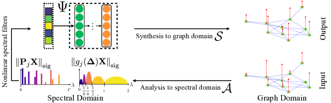
We introduce three novel types of non-linear spectral filters (NLSF): Node-level NLSFs, Graph-level NLSFs, and Pooling-NLSFs. Fig. 1 illustrates our NLSFs for equivariant machine learning on graphs.
Node-level NLSFs. To be able to transfer NLSFs between different graphs and signals, one key property of NLSF is that they do not depend on the specific basis chosen in each eigenspace. This independence is facilitated by the synthesis process, which relies on the input signal . Following the spectral index and filter bank cases in Sec. 3.3, we define the Index NLSFs and Value NLSFs by
| (4) | ||||
| (5) |
where in and in . To adjust the feature output dimension at each node, we apply an MLP with shared weights to all nodes after the NLSF.
Graph-level NLSFs. We first introduce the Graph-level NLSFs that are fully spectral, where the NLSFs map a sequence of frequency coefficients to an output vector. Specifically, the Index-based and Value-based Graph-level NLSFs are given by
| (6) |
where maps from (resp. ) or (resp. ) to , and is the output dimension.
Pooling-NLSFs. We introduce another type of graph-level NLSFs by first representing each graph in a Node-level NLSFs as in Eq. (4) and Eq. (5). The final graph representation is obtained by applying a nonlinear activation function followed by a readout function to these node-level representations. We consider four commonly used pooling methods, including mean, sum, max, and -norm pooling, as the readout function for each graph. We apply an MLP after readout function to obtain a -dimensional graph-level representation. We term these graph-level NLSFs as Pooling-NLSFs.
3.5 Laplacian Attention NLSFs
To understand which Laplacian and parameterization (index v/s value) of the NLSF are preferable in different settings, we follow the random geometric graph analysis outlined in [Paolino et al., 2023]. Specifically, we consider a setting where random geometric graphs are sampled from a metric-probability spaces . In such a case, the graph Laplacian approximates continuous Laplacians on the metric spaces under some conditions. We aim for our NLSFs to produce approximately the same outcome for any two graphs sampled from the same underlying metric space , ensuring that the NLSF is transferable. In App. A.5, we show that if the nodes of the graph are sampled uniformly from , then using the graph Laplacian in Index NLSFs yields a transferable method. Conversely, if the nodes of the graph are sampled non-uniformly, and any two balls of the same radius in have the same volume, then utilizing the normalized graph Laplacian in Value NLSFs is a transferable method.
Given that real-life graphs often fall between these two boundary cases, we present an architecture that chooses between the Index NLSFs and Value NLSFs, as illustrated in Fig. 2. Specifically, a soft attention mechanism is employed to dynamically choose between the two parameterizations, given by
where is obtained using a softmax function to normalize the scores into attention weights, balancing each NLSFs’ contribution. It allows the model to adaptively select the most appropriate parameterization from the graph characteristics, promoting the transferability of the NLSFs.
4 Theoretical Properties of Nonlinear Spectral Filters
We present the desired theoretical properties of our NLSFs at the node-level and graph-level.
4.1 Complexity of NLSFs
NLSFs are implemented by computing the eigenvectors of the GSO. Most existing spectral GNNs avoid direct eigendecomposition due to its perceived inefficiency. Instead, they use filters implemented by applying polynomials [Kipf and Welling, 2016, Defferrard et al., 2016a] or rational functions [Levie et al., 2018, Bianchi et al., 2021] to the GSO in the spatial domain. However, power iteration-based eigendecomposition algorithms, e.g., variants of the Lanczos method, can be highly efficient [Saad, 2011, Lanczos, 1950]. For matrices with non-zero entries, the computational complexity of one iteration for finding eigenvectors corresponding to the smallest or largest eigenvalues (called leading eigenvectors) is . In practice, these eigendecomposition algorithms converge quickly due to their super-exponential convergence rate, often requiring only a few iterations.
This makes NLSFs applicable to node-level tasks on large sparse graphs, as they rely solely on the leading eigenvectors. In Sec. 4.4, we show that using the leading eigenvectors can approximate GSO well in the context of learning on graphs. For node-level tasks, such as semi-supervised node classification, the leading eigenvectors only need to be pre-computed once, with a complexity of . During the learning phase, each step of the architecture search and hyperparameter optimization takes complexity for analysis and synthesis, and for the MLP in the spectral domain, which is faster than the complexity of message passing or standard spectral methods if . Detailed empirical studies on runtime analysis are provided in the App. C.
For dense matrices, the computational complexity of a full eigendecomposition is per iteration, where is the complexity of matrix multiplication. This is practical for graph-level tasks on relatively small and dense graphs, which is typical for many graph classification datasets. In these cases, the eigendecomposition of all graphs in the dataset can be performed as a pre-computation step, significantly reducing the complexity during the learning phase.
4.2 Equivariance of Node-level NLSFs
We demonstrate the node-level equivariance of our NLSFs, ensuring that our method respects the functional shift symmetries. The proof is given in App. A.1.
4.3 Universal Approximation and Expressivity
In this subsection, we discuss the approximation power of NLSFs.
Node-Level Universal Approximation. We begin with a setting where a graph is given as a fixed domain, and the data distribution consists of multiple signals defined on this graph. An example of this setup is a spatiotemporal graph [Cini and Marisca, 2022], e.g., traffic networks, where a fixed sensor system defines a graph and the different signals represent the sensor readings collected at different times.
In App. A.2.1, we prove the following lemma, which shows that linear NLSFs exhaust the space of linear operators that commute with graph functional shifts.
Lemma 4.1.
Lemma 4.1 shows a close relationship between functions that commute with functional shifts and those defined in the spectral domain. This motivates the following construction of a pseudo-metric on . In the case of relaxed functional shifts, we define the standard Euclidean metric in the spectral domain . We pull back the Euclidean metric to the spatial domain to define a signal pseudo-metric. Namely, for two signals and , their distance is defined by
This pseudo metric can be made into a metric by considering each equivalence class of signals with zero distance as a single point in the space. As MLPs can approximate any continuous function (the universal approximation theorem [Cybenko, 1989, Funahashi, 1989, Leshno et al., 1993]), node-level NLSFs can approximate any continuous function that maps (equivalence classes of) signals to (equivalence classes of) signals. For details, see App. A.2.2. A similar analysis applies to hard functional shifts.
Graph-Level Universal Approximation. The above analysis also motivates the construction of a graph-signal metric for graph-level tasks. For graphs with -channel signals, we consider again the standard Euclidean metric in the spectral domain . We define the distance between any two graphs with GSOs and signals and to be
This definition can be extended into a metric by considering the space of equivalence classes of graph-signals with distance 0. As before, this distance inherits the universal approximation properties of standard MLPs. Namely, any continuous function with respect to can be approximated by NLSFs based on MLPs. Additional details are in App. A.2.3.
Graph-Level Expressivity of Pooling-NLSFs. In App. A.2.4, we show that Pooling-NLSFs are more expressive than graph-level NLSF when any norm is used in Eq. (4) and Eq. (5) with , both in the definition of the NLSF and as the pooling method. Specifically, for every graph-level NLSF, there is a Pooling-NLSF that coincides with it. Additionally, there are graph signals and for which a Pooling-NLSF can attain different values, whereas any graph-level NLSF must attain the same value. Hence, Pooling-NLSFs have improved discriminative power compared to graph-level NLSFs. Indeed, as shown in Tab. LABEL:tab:graph_classification_accuracy_vertical, Pooling-NLSFs outperform Graph-level NLSFs in practice, which can be attributed to their increased expressivity.
4.4 Uniform Approximation of GSOs by Their Leading Eigenvectors
Since NLSFs on large graphs are based on the leading eigenvectors of , we justify its low-rank approximation in the following. While approximating matrices with low-rank matrices might lead to a high error in the spectral and Frobenius norms, we show that such an approximation entails a uniformly small error in the cut norm. We define and interpret the cut norm in App. A.4.1, and explain why it is a natural graph similarity measure for graph machine learning.
The following theorem is a corollary of the Constructive Weak Regularity Lemma presented in [Finkelshtein et al., 2024]. Its proof is presented in App. A.4.
Theorem 4.1.
Let be a symmetric matrix with entries bounded by , and let . Suppose is sampled uniformly from , and let s.t. . Let be the leading eigenvectors of , with eigenvalues ordered by their magnitudes . Define . Then, with probability (w.r.t. the choice of ),
5 Experimental Results
We evaluate the NLSFs on node and graph classification tasks. Additional implementation details are in App. B. Additional experiments, including runtime analysis and ablation studies, are in App. C.
5.1 Semi-Supervised Node Classification
| Cora | Citeseer | Pubmed | Chameleon | Squirrel | Actor | |
|---|---|---|---|---|---|---|
| GCN | 81.920.9 | 70.731.1 | 80.140.6 | 43.641.9 | 33.260.8 | 27.631.7 |
| GAT | 83.640.7 | 71.321.3 | 79.450.7 | 42.191.3 | 28.210.9 | 29.460.9 |
| SAGE | 74.012.1 | 66.401.2 | 79.910.9 | 41.920.7 | 27.642.1 | 30.851.8 |
| ChebNet | 79.721.1 | 70.481.0 | 76.471.5 | 44.951.2 | 33.820.8 | 27.422.3 |
| ChebNetII | 83.950.8 | 71.761.2 | 81.381.3 | 46.373.1 | 34.401.1 | 33.481.2 |
| CayleyNet | 81.761.9 | 68.322.3 | 77.482.1 | 38.293.2 | 26.533.3 | 30.622.8 |
| APPNP | 83.190.8 | 71.930.8 | 82.691.4 | 37.431.9 | 25.681.3 | 35.981.3 |
| GPRGNN | 82.821.3 | 70.281.4 | 81.312.6 | 39.272.3 | 26.091.3 | 31.471.6 |
| ARMA | 81.641.2 | 69.911.6 | 79.240.5 | 39.401.8 | 27.420.7 | 30.422.6 |
| -Node-level NLSFs | 84.750.7 | 73.621.1 | 81.931.0 | 49.681.6 | 38.250.7 | 34.720.9 |
We first demonstrate the main advantage of the proposed Node-level NLSFs over existing GNNs with convolution design on semi-supervised node classification tasks. We test three citation networks [Sen et al., 2008, Yang et al., 2016]: Cora, Citeseer, and Pubmed. In addition, we explore three heterophilic graphs: Chameleon, Squirrel, and Actor [Rozemberczki et al., 2021, Tang et al., 2009]. For more comprehensive descriptions of these datasets, see App. B.
We compare the Node-level NLSFs using Laplacian attention with existing spectral GNNs for node-level predictions, including GCN [Kipf and Welling, 2016], ChebNet [Defferrard et al., 2016a], ChebNetII [He et al., 2022], CayleyNet [Levie et al., 2018], APPNP [Klicpera et al., 2019], GPRGNN [Chien et al., 2020], and ARMA [Bianchi et al., 2021]. We also consider GAT [Veličković et al., 2017] and SAGE [Hamilton et al., 2017]. For datasets splitting on citation graphs (Cora, Citeseer, and Pubmed), we apply the standard splits following [Yang et al., 2016], using 20 nodes per class for training, 500 nodes for validation, and 1000 nodes for testing. For heterophilic graphs (Chameleon, Squirrel, and Actor), we use the sparse splitting as in [Chien et al., 2020, He et al., 2022], allocating 2.5% of samples for training, 2.5% for validation, and 95% for testing. We measure the classification quality by computing the average classification accuracy with a 95% confidence interval over 10 random splits. We utilize the source code released by the authors for the baseline algorithms and optimize their hyperparameters using Optuna [Akiba et al., 2019]. Each model’s hyperparameters are fine-tuned to achieve the highest possible accuracy. Detailed hyperparameter settings are provided in App. B.
Tab. LABEL:tab:node_classification_accuracy presents the node classification accuracy of our Node-level NLSFs using Laplacian attention and the various competing baselines. We see that -Node-level NLSFs outperform the competing models on the Cora, Citeseer, and Chameleon datasets. Notably, it shows remarkable performance on the densely connected Squirrel graph, outperforming the baselines by a large margin. This can be explained by the sparse version in Eq. (9) of Thm. 4.1, which shows that the denser the graphs is, the better its rank- approximation. For the Pubmed and Actor datasets, -Node-level NLSFs yield the second-best results, which are comparable to the best results obtained by APPNP.
5.2 Node Classification on Filtered Chameleon and Squirrel Datasets in Dense Split Setting
| Chameleon | Squirrel | ||||
|---|---|---|---|---|---|
| Original | Filtered | Original | Filtered | ||
| ResNet+SGC | 49.932.3 | 41.014.5 | 34.361.2 | 38.362.0 | |
| ResNet+adj | 71.072.2 | 38.673.9 | 65.461.6 | 38.372.0 | |
| GCN | 50.183.3 | 40.894.1 | 39.061.5 | 39.471.5 | |
| GPRGNN | 47.261.7 | 39.933.3 | 33.392.1 | 38.952.0 | |
| FSGNN | 77.850.5 | 40.613.0 | 68.931.7 | 35.921.3 | |
| GloGNN | 70.042.1 | 25.903.6 | 61.212.0 | 35.111.2 | |
| FAGCN | 64.232.0 | 41.902.7 | 47.631.9 | 41.082.3 | |
| -Node-level NLSFs | 79.421.6 | 42.061.3 | 67.811.4 | 42.181.2 | |
Recently, the work in [Platonov et al., 2023] identified the presence of many duplicate nodes across the train, validation, and test splits in the dense split setting of the Chameleon and Squirrel [Pei et al., 2020]. This results in train-test data leakage, causing GNNs to inadvertently fit the test splits during training, thereby making performance results on Chameleon and Squirrel less reliable. To further validate the performance of our Node-level NLSFs on these datasets in the dense split setting, we use both the original and filtered versions of Chameleon and Squirrel, which do not contain duplicate nodes, as suggested in [Platonov et al., 2023]. We use the same random splits as in [Platonov et al., 2023], dividing the datasets into 48% for training, 32% for validation, and 20% for testing.
Tab. 2 presents the classification performance comparison between the original and filtered Chameleon and Squirrel. The baseline results are taken from [Platonov et al., 2023], and we include the following competitive models: ResNet+SGC [Platonov et al., 2023], ResNet+adj [Platonov et al., 2023], GCN [Kipf and Welling, 2016], GPRGNN [Chien et al., 2020], FSGNN [Maurya et al., 2022], GloGNN [Li et al., 2022], and FAGCN [Bo et al., 2021]. The detailed comparisons are in App. C. We see in the table that the -Node-level NLSFs consistently outperform the competing baselines on both the original and filtered datasets. -Node-level NLSFs demonstrate less sensitivity to node duplicates and exhibit stronger generalization ability, further validating the reliability of the Chameleon and Squirrel datasets in the dense split setting. We note that compared to the dense split setting, the sparse split setting in Tab. LABEL:tab:node_classification_accuracy is more challenging, resulting in lower classification performance. A similar trend of significant performance difference between the two settings of Chameleon and Squirrel is also observed in [He et al., 2022].
5.3 Graph Classification
We further illustrate the power of NLSFs on eight graph classification benchmarks [Kersting et al., 2016]. Specifically, we consider five bioinformatics datasets [Borgwardt et al., 2005, Kriege and Mutzel, 2012, Shervashidze et al., 2011]: MUTAG, PTC, NCI1, ENZYMES, and PROTEINS, where MUTAG, PTC, and NCI1 are characterized by discrete node features, while ENZYMES and PROTEINS have continuous node features. Additionally, we examine three social network datasets: IMDB-B, IMDB-M, and COLLAB. The unattributed graphs are augmented by adding node degree features following [Errica et al., 2019]. For more details of these datasets, see App. B.
In graph classification tasks, a readout function is used to summarize node representations for each graph. The final graph-level representation is obtained by aggregating these node-level summaries and is then fed into an MLP with a (log)softmax layer to perform the graph classification task. We compare our NLSFs with two kernel-based approaches: GK [Shervashidze et al., 2009] and WL [Shervashidze et al., 2011], as well as nine GNNs: GCN [Kipf and Welling, 2016], GAT [Veličković et al., 2017], SAGE [Hamilton et al., 2017], ChebNet [Defferrard et al., 2016a], ChebNetII [He et al., 2022], CayleyNet [Levie et al., 2018], APPNP [Klicpera et al., 2019], GPRGNN [Chien et al., 2020], and ARMA [Bianchi et al., 2021]. Additionally, we consider the hierarchical graph pooling model DiffPool [Ying et al., 2018]. For dataset splitting, we apply the random split following [Velickovic et al., 2019, Ying et al., 2018, Ma et al., 2019, Zhu et al., 2021b], using 80% for training, 10% for validation, and 10% for testing. This random splitting process is repeated 10 times, and we report the average performance along with the standard deviation. For the baseline algorithms, we use the source code released by the authors and optimize their hyperparameters using Optuna [Akiba et al., 2019]. We fine-tune the hyperparameters of each model to achieve the highest possible accuracy. Detailed hyperparameter settings for both the baselines and our method are provided in App. B.
| MUTAG | PTC | ENZYMES | PROTEINS | NCI1 | IMDB-B | IMDB-M | COLLAB | |
|---|---|---|---|---|---|---|---|---|
| GK | 76.382.9 | 52.131.2 | 30.076.1 | 72.334.5 | 62.622.2 | 67.631.0 | 44.190.9 | 72.323.7 |
| WL | 78.041.8 | 52.441.3 | 51.295.9 | 76.204.1 | 76.452.3 | 71.423.2 | 46.631.3 | 76.232.2 |
| GCN | 81.633.1 | 60.221.9 | 43.663.4 | 75.173.7 | 76.291.8 | 72.961.3 | 50.283.2 | 79.981.9 |
| GAT | 83.174.4 | 62.311.4 | 39.833.7 | 74.724.1 | 74.014.3 | 70.622.5 | 45.672.7 | 74.272.5 |
| SAGE | 75.184.7 | 61.331.1 | 37.993.7 | 74.014.3 | 74.901.7 | 68.382.6 | 46.942.9 | 73.612.1 |
| DiffPool | 82.401.4 | 56.432.9 | 60.133.2 | 79.473.1 | 77.180.7 | 71.091.6 | 50.431.5 | 80.161.8 |
| ChebNet | 82.151.6 | 64.061.2 | 50.421.4 | 74.280.9 | 76.980.7 | 73.141.1 | 49.821.6 | 77.401.6 |
| ChebNetII | 84.173.1 | 70.032.8 | 64.292.9 | 78.314.1 | 81.143.6 | 77.093.9 | 52.692.7 | 80.063.3 |
| CayleyNet | 83.064.2 | 62.735.1 | 42.285.3 | 74.124.7 | 77.214.5 | 71.454.8 | 51.893.9 | 76.335.8 |
| APPNP | 84.454.4 | 65.266.9 | 49.683.9 | 77.264.8 | 73.247.3 | 72.942.3 | 44.361.9 | 73.853.3 |
| GPRGNN | 80.262.0 | 58.411.4 | 45.291.7 | 73.902.5 | 73.124.0 | 69.172.6 | 47.072.8 | 77.931.9 |
| ARMA | 83.212.7 | 69.232.2 | 61.213.4 | 76.623.6 | 79.512.9 | 73.272.7 | 53.601.9 | 78.341.1 |
| -Graph-level NLSFs | 84.131.5 | 68.171.0 | 65.941.6 | 82.691.9 | 80.511.2 | 74.261.8 | 52.490.7 | 79.061.2 |
| -Pooling-NLSFs | 86.891.2 | 71.021.3 | 69.941.0 | 84.890.9 | 80.951.4 | 76.781.9 | 55.281.7 | 82.191.3 |
Tab. LABEL:tab:graph_classification_accuracy_vertical presents the graph classification accuracy. Notably, the -Graph-level NLSFs (i.e., NLSFs without the synthesis and pooling process) perform the second best on the ENZYMES and PROTEINS. Additionally, -Pooling-NLSFs consistently outperform -Graph-level NLSFs, indicating that the node features learned in our Node-level NLSFs representation are more expressive, corroborating our theoretical findings in Sec. 4.3. Furthermore, our -Pooling-NLSFs consistently outperform all baselines on the MUTAG, PTC, ENZYMES, PROTEINS, IMDB-M, and COLLAB datasets. For NCI1 and IMDB-B, -Pooling-NLSFs rank second and are comparable to ChebNetII.
6 Summary
We presented an approach for defining non-linear filters in the spectral domain of graphs in a transferable and equivariant way. Transferability between different graphs is achieved by using the input signal as a basis for the synthesis operator, making the NLSF depend only on the eigenspaces of the GSO and not on an arbitrary choice of the eigenvectors. While different graph-signals may be of different sizes, the spectral domain is a fixed Euclidean space independent of the size and topology of the graph. Hence, our spectral approach represents graphs as vectors. We note that standard spectral methods do not have this property since the coefficients of the signal in the frequency domain depend on an arbitrary choice of eigenvectors, while our representation depends only on the eigenspaces. We analyzed the universal approximation and expressivity power of NLSFs through metrics that are pulled back from this Euclidean vector space. From a geometric point of view, our NLSFs are motivated by respecting graph functional shift symmetries, making them related to Euclidean CNNs.
Limitation and Future Work. One limitation of NLSFs is that, when deployed on large graphs, they only depend on the leading eigenvectors of the GSO. In this paper, we considered the low-frequency eigenvectors of graph Laplacians. However, important information can also lie within the high frequencies or in any other band. In future work, we plan to explore NLSFs that are sensitive to eigenvalues that lie within a set of bands of interest, which can be adaptive to the graph.
Acknowledgments
The work of YEL and RT was supported by the European Union’s Horizon 2020 research and innovation programme under grant agreement No. 802735-ERC-DIFFOP. The work of RL was supported by the Israel Science Foundation grant #1937/23: Analysis of graph deep learning using graphon theory.
References
- Akiba et al. [2019] Takuya Akiba, Shotaro Sano, Toshihiko Yanase, Takeru Ohta, and Masanori Koyama. Optuna: A next-generation hyperparameter optimization framework. In Proceedings of the 25th ACM SIGKDD international conference on knowledge discovery & data mining, pages 2623–2631, 2019.
- Atz et al. [2021] Kenneth Atz, Francesca Grisoni, and Gisbert Schneider. Geometric deep learning on molecular representations. Nature Machine Intelligence, 3:1023–1032, 2021.
- Barabasi and Oltvai [2004] Albert-Laszlo Barabasi and Zoltan N Oltvai. Network biology: understanding the cell’s functional organization. Nature reviews genetics, 5(2):101–113, 2004.
- Bevilacqua et al. [2022] Beatrice Bevilacqua, Fabrizio Frasca, Derek Lim, Balasubramaniam Srinivasan, Chen Cai, Gopinath Balamurugan, Michael M Bronstein, and Haggai Maron. Equivariant subgraph aggregation networks. In International Conference on Learning Representations, 2022.
- Bianchi et al. [2021] Filippo Maria Bianchi, Daniele Grattarola, Lorenzo Livi, and Cesare Alippi. Graph neural networks with convolutional ARMA filters. IEEE transactions on pattern analysis and machine intelligence, 44(7):3496–3507, 2021.
- Bietti et al. [2021] Alberto Bietti, Luca Venturi, and Joan Bruna. On the sample complexity of learning with geometric stability. arXiv preprint arXiv:2106.07148, 2021.
- Bo et al. [2021] Deyu Bo, Xiao Wang, Chuan Shi, and Huawei Shen. Beyond low-frequency information in graph convolutional networks. In Proceedings of the AAAI conference on artificial intelligence, volume 35, pages 3950–3957, 2021.
- Borgatti et al. [2009] Stephen P Borgatti, Ajay Mehra, Daniel J Brass, and Giuseppe Labianca. Network analysis in the social sciences. science, 323(5916):892–895, 2009.
- Borgwardt et al. [2005] Karsten M Borgwardt, Cheng Soon Ong, Stefan Schönauer, SVN Vishwanathan, Alex J Smola, and Hans-Peter Kriegel. Protein function prediction via graph kernels. Bioinformatics, 21(suppl_1):i47–i56, 2005.
- Bracewell and Kahn [1966] Ron Bracewell and Peter B Kahn. The fourier transform and its applications. American Journal of Physics, 34(8):712–712, 1966.
- Bronstein et al. [2017] M. M. Bronstein, J. Bruna, Y. LeCun, A. Szlam, and P. Vandergheynst. Geometric deep learning: Going beyond euclidean data. IEEE Signal Processing Magazine, 34(4):18–42, 2017.
- Bronstein et al. [2021] Michael M Bronstein, Joan Bruna, Taco Cohen, and Petar Veličković. Geometric deep learning: Grids, groups, graphs, geodesics, and gauges. preprint arXiv:2104.13478, 2021.
- Bruna et al. [2013] Joan Bruna, Wojciech Zaremba, Arthur Szlam, and Yann LeCun. Spectral networks and locally connected networks on graphs. arXiv preprint arXiv:1312.6203, 2013.
- Chien et al. [2020] Eli Chien, Jianhao Peng, Pan Li, and Olgica Milenkovic. Adaptive universal generalized pagerank graph neural network. In International Conference on Learning Representations, 2020.
- Cini and Marisca [2022] Andrea Cini and Ivan Marisca. Torch Spatiotemporal, 3 2022.
- Cohen and Welling [2016] Taco Cohen and Max Welling. Group equivariant convolutional networks. In ICML, pages 2990–2999. PMLR, 2016.
- Cybenko [1989] George Cybenko. Approximation by superpositions of a sigmoidal function. Mathematics of control, signals and systems, 2(4):303–314, 1989.
- Defferrard et al. [2016a] Michaël Defferrard, Xavier Bresson, and Pierre Vandergheynst. Convolutional neural networks on graphs with fast localized spectral filtering. Advances in neural information processing systems, 29, 2016a.
- Defferrard et al. [2016b] Michaël Defferrard, Xavier Bresson, and Pierre Vandergheynst. Convolutional neural networks on graphs with fast localized spectral filtering. In NeurIPS. Curran Associates Inc., 2016b. ISBN 9781510838819.
- Du et al. [2022] Lun Du, Xiaozhou Shi, Qiang Fu, Xiaojun Ma, Hengyu Liu, Shi Han, and Dongmei Zhang. Gbk-gnn: Gated bi-kernel graph neural networks for modeling both homophily and heterophily. In Proceedings of the ACM Web Conference 2022, pages 1550–1558, 2022.
- Duval et al. [2024] Alexandre Duval, Simon V. Mathis, Chaitanya K. Joshi, Victor Schmidt, Santiago Miret, Fragkiskos D. Malliaros, Taco Cohen, Pietro Liò, Yoshua Bengio, and Michael Bronstein. A hitchhiker’s guide to geometric gnns for 3d atomic systems, 2024.
- Elesedy and Zaidi [2021] Bryn Elesedy and Sheheryar Zaidi. Provably strict generalisation benefit for equivariant models. ICML, 2021.
- Errica et al. [2019] Federico Errica, Marco Podda, Davide Bacciu, and Alessio Micheli. A fair comparison of graph neural networks for graph classification. In International Conference on Learning Representations, 2019.
- Fey and Lenssen [2019] Matthias Fey and Jan E. Lenssen. Fast graph representation learning with PyTorch Geometric. In ICLR Workshop on Representation Learning on Graphs and Manifolds, 2019.
- Finkelshtein et al. [2024] Ben Finkelshtein, Ismail Ilkan Ceylan, Michael M. Bronstein, and Ron Levie. Learning on Large Graphs using Intersecting Communities. 2024.
- Frasca et al. [2022] Fabrizio Frasca, Beatrice Bevilacqua, Michael Bronstein, and Haggai Maron. Understanding and extending subgraph GNN by rethinking their symmetries. Advances in Neural Information Processing Systems, 35:31376–31390, 2022.
- Frieze and Kannan [1999] Alan M. Frieze and Ravi Kannan. Quick approximation to matrices and applications. Combinatorica, 1999.
- Funahashi [1989] Ken-Ichi Funahashi. On the approximate realization of continuous mappings by neural networks. Neural networks, 2(3):183–192, 1989.
- Gaudelet et al. [2021] Thomas Gaudelet, Ben Day, Arian R Jamasb, Jyothish Soman, Cristian Regep, Gertrude Liu, Jeremy BR Hayter, Richard Vickers, Charles Roberts, Jian Tang, et al. Utilizing graph machine learning within drug discovery and development. Briefings in bioinformatics, 22(6):bbab159, 2021.
- Gilmer et al. [2017] Justin Gilmer, Samuel S Schoenholz, Patrick F Riley, Oriol Vinyals, and George E Dahl. Neural message passing for quantum chemistry. In International conference on machine learning, pages 1263–1272. PMLR, 2017.
- Hamilton et al. [2017] Will Hamilton, Zhitao Ying, and Jure Leskovec. Inductive representation learning on large graphs. Advances in Neural Information Processing Systems, 30, 2017.
- He et al. [2016] Kaiming He, Xiangyu Zhang, Shaoqing Ren, and Jian Sun. Deep residual learning for image recognition. In Proceedings of the IEEE conference on computer vision and pattern recognition, pages 770–778, 2016.
- He et al. [2022] Mingguo He, Zhewei Wei, and Ji-Rong Wen. Convolutional neural networks on graphs with chebyshev approximation, revisited. Advances in Neural Information Processing Systems, 35:7264–7276, 2022.
- Huang et al. [2024] Ningyuan Huang, Ron Levie, and Soledad Villar. Approximately equivariant graph networks. Advances in Neural Information Processing Systems, 36, 2024.
- Jumper et al. [2021] John M. Jumper, Richard Evans, Alexander Pritzel, Tim Green, Michael Figurnov, Olaf Ronneberger, Kathryn Tunyasuvunakool, Russ Bates, Augustin Zídek, Anna Potapenko, Alex Bridgland, Clemens Meyer, Simon A A Kohl, Andy Ballard, Andrew Cowie, Bernardino Romera-Paredes, Stanislav Nikolov, Rishub Jain, Jonas Adler, Trevor Back, Stig Petersen, David A. Reiman, Ellen Clancy, Michal Zielinski, Martin Steinegger, Michalina Pacholska, Tamas Berghammer, Sebastian Bodenstein, David Silver, Oriol Vinyals, Andrew W. Senior, Koray Kavukcuoglu, Pushmeet Kohli, and Demis Hassabis. Highly accurate protein structure prediction with alphafold. Nature, 596:583 – 589, 2021.
- Kersting et al. [2016] Kristian Kersting, Nils M Kriege, Christopher Morris, Petra Mutzel, and Marion Neumann. Benchmark data sets for graph kernels. 2016.
- Kingma and Ba [2014] Diederik P Kingma and Jimmy Ba. Adam: A method for stochastic optimization. arXiv preprint arXiv:1412.6980, 2014.
- Kipf and Welling [2016] Thomas N Kipf and Max Welling. Semi-supervised classification with graph convolutional networks. In International Conference on Learning Representations, 2016.
- Klicpera et al. [2019] Johannes Klicpera, Aleksandar Bojchevski, and Stephan Günnemann. Predict then propagate: Graph neural networks meet personalized pagerank. In International Conference on Learning Representations, 2019. URL https://openreview.net/forum?id=H1gL-2A9Ym.
- Kriege and Mutzel [2012] Nils Kriege and Petra Mutzel. Subgraph matching kernels for attributed graphs. arXiv preprint arXiv:1206.6483, 2012.
- Krizhevsky et al. [2012] Alex Krizhevsky, Ilya Sutskever, and Geoffrey E Hinton. Imagenet classification with deep convolutional neural networks. In Advances in Neural Information Processing Systems, volume 25. Curran Associates, Inc., 2012.
- Lanczos [1950] Cornelius Lanczos. An iteration method for the solution of the eigenvalue problem of linear differential and integral operators. 1950.
- LeCun et al. [1995] Yann LeCun, Yoshua Bengio, et al. Convolutional networks for images, speech, and time series. The handbook of brain theory and neural networks, 3361(10):1995, 1995.
- LeCun et al. [2010] Yann LeCun, Koray Kavukcuoglu, and Clément Farabet. Convolutional networks and applications in vision. In Proceedings of 2010 IEEE international symposium on circuits and systems, pages 253–256. IEEE, 2010.
- Leshno et al. [1993] Moshe Leshno, Vladimir Ya Lin, Allan Pinkus, and Shimon Schocken. Multilayer feedforward networks with a nonpolynomial activation function can approximate any function. Neural networks, 6(6):861–867, 1993.
- Levie et al. [2021] R. Levie, W. Huang, L. Bucci, M. Bronstein, and G. Kutyniok. Transferability of spectral graph convolutional neural networks. Journal of Machine Learning Research, 22(272):1–59, 2021.
- Levie [2023] Ron Levie. A graphon-signal analysis of graph neural networks. In NeurIPS, 2023.
- Levie et al. [2018] Ron Levie, Federico Monti, Xavier Bresson, and Michael M Bronstein. Cayleynets: Graph convolutional neural networks with complex rational spectral filters. IEEE Transactions on Signal Processing, 67(1):97–109, 2018.
- Li et al. [2022] Xiang Li, Renyu Zhu, Yao Cheng, Caihua Shan, Siqiang Luo, Dongsheng Li, and Weining Qian. Finding global homophily in graph neural networks when meeting heterophily. In International Conference on Machine Learning, pages 13242–13256. PMLR, 2022.
- Lim et al. [2024] Derek Lim, Joshua Robinson, Stefanie Jegelka, and Haggai Maron. Expressive sign equivariant networks for spectral geometric learning. Advances in Neural Information Processing Systems, 36, 2024.
- Lovász and Szegedy [2007] László Lovász and Balázs Szegedy. Szemerédi’s lemma for the analyst. GAFA Geometric And Functional Analysis, 2007.
- Lovász [2012] László Miklós Lovász. Large networks and graph limits. In volume 60 of Colloquium Publications, 2012.
- Ma et al. [2019] Yao Ma, Suhang Wang, Charu C Aggarwal, and Jiliang Tang. Graph convolutional networks with eigenpooling. In Proceedings of the 25th ACM SIGKDD international conference on knowledge discovery & data mining, pages 723–731, 2019.
- Mallat [1989] Stephane G Mallat. A theory for multiresolution signal decomposition: the wavelet representation. IEEE transactions on pattern analysis and machine intelligence, 11(7):674–693, 1989.
- Maurya et al. [2022] Sunil Kumar Maurya, Xin Liu, and Tsuyoshi Murata. Simplifying approach to node classification in graph neural networks. Journal of Computational Science, 62:101695, 2022.
- Méndez-Lucio et al. [2021] Oscar Méndez-Lucio, Mazen Ahmad, Ehecatl Antonio del Rio-Chanona, and Jörg Kurt Wegner. A geometric deep learning approach to predict binding conformations of bioactive molecules. Nature Machine Intelligence, 3:1033–1039, 2021.
- Morris et al. [2020] Christopher Morris, Nils M Kriege, Franka Bause, Kristian Kersting, Petra Mutzel, and Marion Neumann. Tudataset: A collection of benchmark datasets for learning with graphs. arXiv preprint arXiv:2007.08663, 2020.
- Ovsjanikov et al. [2012] Maks Ovsjanikov, Mirela Ben-Chen, Justin Solomon, Adrian Butscher, and Leonidas Guibas. Functional maps: A flexible representation of maps between shapes. ACM Transactions on Graphics (ToG), 31(4):1–11, 2012.
- Paolino et al. [2023] Raffaele Paolino, Aleksandar Bojchevski, Stephan Günnemann, Gitta Kutyniok, and Ron Levie. Unveiling the sampling density in non-uniform geometric graphs. In The Eleventh International Conference on Learning Representations, 2023.
- Pei et al. [2020] Hongbin Pei, Bingzhe Wei, Kevin Chen-Chuan Chang, Yu Lei, and Bo Yang. Geom-gcn: Geometric graph convolutional networks. In International Conference on Learning Representations, 2020.
- Petrache and Trivedi [2024] Mircea Petrache and Shubhendu Trivedi. Approximation-generalization trade-offs under (approximate) group equivariance. Advances in Neural Information Processing Systems, 36, 2024.
- Platonov et al. [2023] Oleg Platonov, Denis Kuznedelev, Michael Diskin, Artem Babenko, and Liudmila Prokhorenkova. A critical look at the evaluation of gnns under heterophily: Are we really making progress? In The Eleventh International Conference on Learning Representations, 2023.
- Rozemberczki et al. [2021] Benedek Rozemberczki, Carl Allen, and Rik Sarkar. Multi-scale attributed node embedding. Journal of Complex Networks, 9(2):cnab014, 2021.
- Saad [2011] Yousef Saad. Numerical methods for large eigenvalue problems: revised edition. SIAM, 2011.
- Scarselli et al. [2008] Franco Scarselli, Marco Gori, Ah Chung Tsoi, Markus Hagenbuchner, and Gabriele Monfardini. The graph neural network model. IEEE transactions on neural networks, 20(1):61–80, 2008.
- Sen et al. [2008] Prithviraj Sen, Galileo Namata, Mustafa Bilgic, Lise Getoor, Brian Galligher, and Tina Eliassi-Rad. Collective classification in network data. AI magazine, 29(3):93–93, 2008.
- Serre et al. [1977] Jean-Pierre Serre et al. Linear representations of finite groups, volume 42. Springer, 1977.
- Shervashidze et al. [2009] Nino Shervashidze, SVN Vishwanathan, Tobias Petri, Kurt Mehlhorn, and Karsten Borgwardt. Efficient graphlet kernels for large graph comparison. In Artificial intelligence and statistics, pages 488–495. PMLR, 2009.
- Shervashidze et al. [2011] Nino Shervashidze, Pascal Schweitzer, Erik Jan Van Leeuwen, Kurt Mehlhorn, and Karsten M Borgwardt. Weisfeiler-Lehman graph kernels. Journal of Machine Learning Research, 12(9), 2011.
- Shi et al. [2020] Yunsheng Shi, Zhengjie Huang, Shikun Feng, Hui Zhong, Wenjin Wang, and Yu Sun. Masked label prediction: Unified message passing model for semi-supervised classification. arXiv preprint arXiv:2009.03509, 2020.
- Stokes et al. [2020] Jonathan M Stokes, Kevin Yang, Kyle Swanson, Wengong Jin, Andres Cubillos-Ruiz, Nina M Donghia, Craig R MacNair, Shawn French, Lindsey A Carfrae, Zohar Bloom-Ackermann, et al. A deep learning approach to antibiotic discovery. Cell, 180(4):688–702, 2020.
- Tang et al. [2009] Jie Tang, Jimeng Sun, Chi Wang, and Zi Yang. Social influence analysis in large-scale networks. In Proceedings of the 15th ACM SIGKDD international conference on Knowledge discovery and data mining, pages 807–816, 2009.
- Trefethen and Bau [2022] Lloyd N. Trefethen and David Bau. Numerical Linear Algebra, Twenty-fifth Anniversary Edition. Society for Industrial and Applied Mathematics, 2022.
- Veličković et al. [2017] Petar Veličković, Guillem Cucurull, Arantxa Casanova, Adriana Romero, Pietro Lio, and Yoshua Bengio. Graph attention networks. arXiv preprint arXiv:1710.10903, 2017.
- Velickovic et al. [2019] Petar Velickovic, William Fedus, William L Hamilton, Pietro Liò, Yoshua Bengio, and R Devon Hjelm. Deep graph infomax. ICLR, 2(3):4, 2019.
- Villar et al. [2023] Soledad Villar, David W Hogg, Weichi Yao, George A Kevrekidis, and Bernhard Schölkopf. Towards fully covariant machine learning. arXiv preprint arXiv:2301.13724, 2023.
- Wang and Zhang [2022] Xiyuan Wang and Muhan Zhang. How powerful are spectral graph neural networks. In International Conference on Machine Learning, pages 23341–23362. PMLR, 2022.
- Wang et al. [2019] Yue Wang, Yongbin Sun, Ziwei Liu, Sanjay E Sarma, Michael M Bronstein, and Justin M Solomon. Dynamic graph cnn for learning on point clouds. ACM Transactions on Graphics (tog), 38(5):1–12, 2019.
- Wu et al. [2020] Zonghan Wu, Shirui Pan, Fengwen Chen, Guodong Long, Chengqi Zhang, and S Yu Philip. A comprehensive survey on graph neural networks. IEEE transactions on neural networks and learning systems, 32(1):4–24, 2020.
- Yang et al. [2016] Zhilin Yang, William Cohen, and Ruslan Salakhudinov. Revisiting semi-supervised learning with graph embeddings. In International conference on machine learning, pages 40–48. PMLR, 2016.
- Ying et al. [2018] Zhitao Ying, Jiaxuan You, Christopher Morris, Xiang Ren, Will Hamilton, and Jure Leskovec. Hierarchical graph representation learning with differentiable pooling. Advances in neural information processing systems, 31, 2018.
- Zhu et al. [2020] Jiong Zhu, Yujun Yan, Lingxiao Zhao, Mark Heimann, Leman Akoglu, and Danai Koutra. Beyond homophily in graph neural networks: Current limitations and effective designs. Advances in neural information processing systems, 33:7793–7804, 2020.
- Zhu et al. [2021a] Jiong Zhu, Ryan A Rossi, Anup Rao, Tung Mai, Nedim Lipka, Nesreen K Ahmed, and Danai Koutra. Graph neural networks with heterophily. In Proceedings of the AAAI conference on artificial intelligence, volume 35, pages 11168–11176, 2021a.
- Zhu et al. [2021b] Yanqiao Zhu, Yichen Xu, Feng Yu, Qiang Liu, Shu Wu, and Liang Wang. Graph contrastive learning with adaptive augmentation. In Proceedings of the Web Conference 2021, pages 2069–2080, 2021b.
Appendix A Theoretical Analysis
We note that the numbering of the statements corresponds to the numbering used in the paper, and we have also included several separately numbered propositions and lemmas that are used in supporting the proofs presented. We restate the claim of each statement for convenience.
A.1 Equivariance of NLSFs
We start with two lemmas that characterize the graph functional shifts. The lemmas directly follow the fact that two normal operators commute iff the projections upon their eigenspaces commute.
Projection to Eigenspaces Case.
Denote by the span of . Denote by the orthonormal complement of . Note that
where and denote direct products of linear spaces. Denote by the direct sum of operators.
Lemma A.1.
is in iff it has the form , where is a unitary operator in , and a unitary operator in .
Projection to Bands Case.
Denote by the span of . Denote by the orthonormal complement of . Note that
Lemma A.2.
is in iff it has the form , where is a unitary operator in , and a unitary operator in .
A.1.1 Proof of Propositions 4.1
Proposition 4.1.
Index NLSFs in Eq. (4) are equivariant to the graph functional shift , and Value NLSFs in Eq. (5) are equivariant to the relaxed graph functional shifts .
Proof.
We start with Index-NLSFs. Consider the Index NLSFs defined as in Eq. (4)
We need to show that for any unitary operator ,
Consider and apply it to the graph signal , the Index NLSFs with the transformed input is given by
Since , it commutes with for all , i.e., . Using this commutation property, we can rewrite the norm and the projections:
In addition, since is a unitary matrix, it preserves the norm. Therefore, we have
Substitute these expressions back into the definition of the Index NLSFs:
Notice that appears linearly in the numerator of the fraction. We can factor it out:
The expression inside the summation is exactly the original Index NLSFs applied to
Therefore, we have shown that applying the unitary operator to the graph signal results in the Index NLSFs being transformed by the same unitary operator , proving the equivariance property.
The proof for value-NLSF follows the same steps. ∎
A.2 Expressivity and Universal Approximation
In this section, we focus on value parameterized NLSFs. The analysis for index-NLSF is equivalent.
A.2.1 Proof of Lemma 4.1 - Linear Node-level NLSF Exhaust the Linear Operators that Commute with Functional Shifts
Lemma 4.1
Suppose that . A linear operator commute with (resp. ) iff it is a NLSF based on a linear function in Eq. (4) (resp. Eq. (5)).
Proof.
Consider a setting where a single graph is given as a fixed domain, and the data distribution consists of many signals defined on this graph. For simplicity, we restrict the analysis to the case of 1D signals (). The extension to a general dimension is natural.
We next show that node-level linear NLSFs exhaust the space of linear operators that commute with graph functional shifts (on the fixed graph).
By Lemma A.2, any unitary operator in has the form
where is a unitary operator in , and a unitary operator in .
Hence, since the unitary representation of the group of unitary operators in is irreducible, by Schur’s lemma [Serre et al., 1977] any linear operator that commutes with all operators of must be a scalar times the identity when projected to and to . Namely, has the form
where is the identity operator in , is the identity operator in , and and are scalars. This means that linear node-level NLSFs exhaust the space of linear operators that commute with .
The case of hard graph functional shifts is treated similarly. ∎
NLSF with High Frequency Content.
We note that the condition can be omitted from Lemma 4.1 if we extend the definition of NLSF by adding one more term in the spectrum as follows. In the spectral index case, concatenate to the analysis operator the coefficient , and in the value case, concatenate . Extend accordingly the definition of synthesis and of NLSFs to also depend on this term. We do not include this spectral term in practice as it does not lead to improved performance.
A.2.2 Node-Level Universal Approximation
The above analysis motivates the following construction of a metric on . Given the filter bank , on graph with -dimensional signals, we define the standard Euclidean metric in the spectral domain . We pull back the Euclidean metric to the spatial domain to define a graph-signal metric. Namely, for two signals and , their distance is defined to be
This defines a pseudometric on the space of graph-signals. To obtain a metric, we consider each equivalence class of signals with zero distance as a single point. Namely, we define the space to be the space of signals with 1D features modulo . In , the pseudometric becomes a metric, and an isometry of metric spaces222 operates on an equivalence class of signals by applying on an arbitrary element of . The output of on does not depend on the specific representative , but only on ..
Now, since MLPs can approximate any continuous function (by the universal approximation theorem), and by the fact that is an isometry, node-level NLSFs based on MLPs in the spectral domain can approximate any continuous function from signals with features to signal with features .
A.2.3 Graph-Level Universal approximation
The above analysis also motivates the construction of a graph-signal metric for graph-level tasks. For graphs with -channel signals, we define the standard Euclidean metric in the spectral domain . We pull back the Euclidean metric to the spatial domain to define a graph-signal metric. Namely, for two graphs with Laplacians and signals and , their distance is defined to be
This defines a pseudometric on the space of graph-signals. To obtain a metric, we consider equivalence classes of graph-signals with zero distance as a single point. Namely, we define the space to be the space of graph-signal modulo . In , the function becomes a metric, and an isometry.
By the isometry property, inherits any approximation property from . For example, since MLPs can approximate any continuous function , the space of NLSFs based on MLPs has a universality property: any continuous function with respect to can be approximated by a NLSF based on an MLP.
A.2.4 Graph-Level Expressivity of Pooling-NLSFs
We now show that pooling-NLSF are more expressive than graph-level NLSF if the norm in Eq. (4) and Eq. (5) is with .
First, we show that there are graph-signals that graph-level-NLSFs cannot separate and Pooling-NLSFs can. Consider an index NLSF with norm normalize by . Namely, for ,
The general case is similar.
For the two graphs, take the graph Laplacian
with eigenvalues , and corresponding eigenvectors and . Take the graph Laplacian
with eigenvalues . The first two eigenvectors are and respectively.
Consider an Index-NLSF based on two eigenprojections . As the signal of the first graph take , and for the second graph take . Both graph-signals have the same spectral coefficients , so graph-level NLSF cannot separate them. Suppose that the NLSF is
The outcome of the corresponding Pooling NLSF on the two graphs is
Hence, Pooling-NLSFs separate these inputs, while graph-level-NLSFs do not.
Next, we show that Pooling-NLSFs are at least as expressive as graph-level NLSFs. In particular, any graph-level NLSF can be expressed as a pooling NLSF.
Let be a graph-level NLSF. Define the node-level NLSF that chooses one spectral index with a nonzero value (e.g., the band with the largest coefficient) and projects upon it the value . Hence, before pooling, the NLSF gives
where depends on the spectral coefficients (e.g., it is the index of the largest spectral coefficient). Hence, after pooling, the Pooling NLSF returns , which coincides with the output of the graph-level NLSF.
Now, let us show that for , they have the same expressivity. For any NLSF,
This is a generic fully spectral NLSF.
A.3 Stable Invertibility of Synthesis
In the fixed graph setting, given any signal such that for every , the synthesis operator is stably invertible. Indeed, the right singular vectors of are the standard basis elements in , the left singular vectors are
and the singular values are
for . Hence, we have
and
Suppose that and . In this case, is an isometry from the spectral domain to a subspace of the signal space . Analysis is the adjoint of synthesis.
This analysis can be extended to the index parametrization case.
A.4 Uniform Approximation of Graphs with Eigenvectors
In this section, we develop the setting under which the low-rank approximation of GSOs with their leading eigenvectors can be interpreted as a uniform approximation (Sec. 4.4).
A.4.1 Cut Norm
The cut norm of is defined to be
| (7) |
The distance between two matrices in cut norm is defined to be .
The cut norm has the following interpretation, which has precise formulation in terms of the weak regularity lemma [Frieze and Kannan, 1999, Lovász and Szegedy, 2007]. Any pair of (deterministic) graphs are close to each other in cut norm if and only if they can be described as pseudo-random graphs sampled from the same stochastic block model. Hence, the cut norm is a meaningful notion of graph similarity for practical graph machine learning, where graphs are noisy and can represent the same underlying phenomenon even if they have different sizes and topologies. In addition, the distance between non-isomorphic graphons is always positive in cut norm [Lovász, 2012]. In this context, the work in [Levie, 2023] showed that GNNs with normalized sum aggregation cannot separate graphs that have zero distance in the cut norm. This means that the cut norm is sufficiently discriminative for practical machine learning on graphs.
A.4.2 The Constructive Weak Regularity Lemma in Hilbert Spaces
The following lemma, called the constructive weak regularity lemma in Hilbert spaces, was proven in [Finkelshtein et al., 2024]. It is an extension of the classical respective result from [Lovász and Szegedy, 2007].
We define the Frobenius norm normalized by as
Lemma A.3.
[[Finkelshtein et al., 2024]] Let be a sequence of nonempty subsets of a real Hilbert space and let . Let , let such that , and let . Let be randomly uniformly sampled from . Then, in probability (with respect to the choice of ), any vector of the form
that gives a close-to-best Hilbert space approximation of in the sense that
| (8) |
where the infimum is over and , also satisfies
A.4.3 Proof of Theorem 4.1
Theorem 4.1.
Let be a symmetric matrix with entries bounded by , and let . Suppose is sampled uniformly from , and let s.t. . Consider as the leading eigenvectors of , with eigenvalues ordered by their magnitudes . Define . Then, with probability (w.r.t. the choice of ),
Proof.
Let us use Lemma A.3, with , and the set of symmetric rank one matrices of the form where is a column vector. Denote by the space of linear combinations of elements of , which is the space of symmetric matrices of rank bounded by . For the Hilbert space norm, we take the Frobenius norm. In the setting of the lemma, we take , and , and . By the lemma, with probability , any Frobenius minimizer , namely, that satisfies , also satisfies
for every . Hence, for every choice of subset , we have
where for a set , denote by the column vector with at coordinates in and otherwise.
Hence, we also have
Lastly, note that by the best rank- approximation theorem (Eckart–Young–Mirsky Theorem [Trefethen and Bau, 2022, Thm. 5.9]), any Frobenius minimizer is the projection upon the leading eigenvectors of (or some choice of these eigenvectors in case of multiplicity higher than 1).
∎
Now, one can use the adjacency matrix as in Thm. 4.1. When working with sparse matrices of edges, to achieve a meaningful scaling of cut distance, we re-normalize the cut norm and define
With this norm, Thm. 4.1 gives
| (9) |
While this bound is not uniformly small in , it is still independent of . In contrast, the error bounds for spectral and Frobenius norms do depend on the specific properties of .
Now, if we want to apply Thm. 4.1 to other GSOs , we need to make some assumptions. Note that when the GSO is a Laplacian, we take as the leading eigenvectors the ones correspoding to the smallest eigenvalues, not the largest ones. To make the theorem applicable, we need to reorder the eigenvectors of . This can be achieved by applying a decreasing function to , such as . The role of is to amplify the eigenspaces of in which most of the energy of signals interest (the ones that often appear in the dataset) is concentrated. Under the assumption that has entries bounded by some not-too-high , one can now justify approximating GSOs by low-rank approximations based on the smallest eigenvectors.
A.5 NLSFs on Random Geometric Graphs
In this section we consider the norm normalized by , namely,
We follow a similar analysis to [Paolino et al., 2023], mostly skipping the rigorous Monte-Carlo error rate proofs, as these are standard. Let be a metric space with metric and with a Borel probability measure, that we call the uniform measure . Let , and denote by the ball of radius about . Let be the volume of with respect to the uniform measure. We consider an underlying Laplacian on the space defined on signals by
where we assume in the analysis below without loss of generality. Note that is compact, so it has a discrete spectrum.
Let be a emasurable weight matrix with . Suppose that is continuous and varies slowly over . Namely, we assume that for every . To generate a random geomertic graph of nodes, we sample points independently from the weighted measure . We connect node to be an edge if and only if to obtain the adjacency matrix . The number of samples inside the ball of radius around is approximately . Hence, the degree of the node is approximately .
We consider the leading eigenvectors of and , where , namely, the eigenvectors corresponding to the largest eigenvalues in their absolute value. We order the eigenvalues in decreasing order from positive to negative. Let be the space spanned by the leading eigenvectors of , called the Paley-Wiener space of . Let be the projection upon the Paley-Wiener space of . Let be the sampling operator, defined by .
Let be a bounded signal over the metric space and suppose that . Denote . By Monte Carlo theory, we have
So, in case the sampling is uniform. i.e. , we have
pointwise. To make this precise, let us recall Hoeffding’s Inequality.
Theorem A.1 (Hoeffding’s Inequality).
Let be independent random variables such that almost surely. Then, for every ,
Using Hoeffding’s Inequality, one can now show that there is an event of probability more than in which for every , the error between and satisfies
The fact that different graphs of different sizes approximate with different scaling factors means that is not value transferable. Let us show that is index transferable.
We now evoke the transferability theorem – a slight reformulation of Section 3 of Theorem 4 in [Levie et al., 2021].
Theorem A.2.
Let be a compact operator on and an operator on . Let and let be the sampling operator defined above. Let be the space spanned by the leading eigenvectors of , and let . Let be Lipschitz with Lipschitz constant . Then, there exists a constant (that depends on ) such that
For every leading eigenvalue of let be the leading eigenvalue of closest to , where, if there are repeated eigenvalues, is chosen arbitrarily out of the eigenvalues of that best approximate .Let
where
and
and suppose that . For each there exists a Lipschitz continuous function with Lipschitz constant such that and is zero on all other leading eigenvalues of and all other eigenvalues of . Hence,
where is the projection upon the space spanned by the -th eigenvector of , and is the projection upon the space spanned by the -th eigenvector of .
Now, be the transferability theorem,
By induction over , with base , we must have for every .
Now, note that by standard Monte Carlo theory (evoking Hoeffding’s inequality again and intersecting events), we have
in high probability. Hence, by the fact that
and is bounded from below by the constant ,
This shows that
which shows index transferability. Namely, for two graphs of and nodes sampled from , with corresponding Laplacians and , by the triangle inequality,
Next, we show value transferability for . Here,
Hence, if is constant, we have up to a constant that does not depend on . In this case, by a similar analysis to the above, is value transferable. We note that is also index transferable, but value transferability is guaranteed in a more general case, where we need not assume a separable spectrum.
Appendix B Additional Details on Experimental Study
We describe the experimental setups and additional details of our experiments in Sec. 5.
B.1 Semi-Supervised Node Classification
We provide a detailed overview of the experimental settings for semi-supervised node classification tasks, along with the validated hyperparameters used in our benchmarks.
Datasets. We consider six datasets in node classification tasks, including Cora, Citeseer, Pubmed, Chameleon, Squirrel, and Actor. The detailed statistics of the node classification benchmarks are summarized in Tab. LABEL:tab:node_classification_statistics. For datasets splitting on citation graphs (Cora, Citeseer, and Pubmed), we follow the standard splits from [Yang et al., 2016], using 20 nodes per class for training, 500 nodes for validation, and 1000 nodes for testing. For heterophilic graphs (Chameleon, Squirrel, and Actor), we adopt the sparse splitting method from [Chien et al., 2020, He et al., 2022], allocating 2.5% of samples for training, 2.5% for validation, and 95% for testing. The classification quality is assessed by computing the average classification accuracy across 10 random splits, along with a 95% confidence interval.
Baselines. For GCN, GAT, SAGE, ChebNet, ARMA, and APPNP, we use the implementations from the PyTorch Geometric library [Fey and Lenssen, 2019]. For other baselines, we use the implementations released by the respective authors.
Hyperparameters Settings. The hidden dimension is set to be either 64 or 128 for all models and datasets. We implement our proposed Node-level NLSFs using PyTorch and optimize the model with the Adam optimizer [Kingma and Ba, 2014]. To determine the optimal dropout probability, we search within the range in increments of . The learning rate is examined within the set . We explore weight decay values within the set . Furthermore, the number of layers is varied from 1 to 10. The number of leading eigenvectors in Index NLSFs is set within . The decay rate in the Value NLSFs is determined using dyadic sampling within the set , the sampling resolution within , and the number of the bands in Value NLSFs . For hyperparameter optimization, we conduct a grid search using Optuna [Akiba et al., 2019] for each dataset. An early stopping criterion is employed during training, stopping the process if the validation loss does not decrease for 200 consecutive epochs.
| Dataset | Nodes | Classes | Edges | Features |
|---|---|---|---|---|
| Cora | 2708 | 7 | 5278 | 1433 |
| Citeseer | 3327 | 6 | 4552 | 3703 |
| Pubmed | 19717 | 5 | 44324 | 500 |
| Chameleon | 2277 | 5 | 31371 | 2325 |
| Squirrel | 5201 | 5 | 198353 | 2089 |
| Actor | 7600 | 5 | 26659 | 932 |
B.2 Graph Classification
| Dataset | Graphs () | Classes () | Features () | |||
| MUTAG | 188 | 2 | 10 | 28 | 17.93 | 7 |
| PTC | 344 | 2 | 2 | 64 | 14.29 | 18 |
| ENZYMES | 600 | 6 | 2 | 126 | 32.63 | 18 |
| PROTEINS | 1113 | 2 | 4 | 620 | 39.06 | 29 |
| NCI1 | 4110 | 2 | 3 | 111 | 29.87 | 37 |
| IMDB-B | 1000 | 2 | 12 | 136 | 19.77 | None |
| IMDB-M | 1500 | 3 | 7 | 89 | 13.00 | None |
| COLLAB | 5000 | 3 | 32 | 492 | 74.50 | None |
We provide a comprehensive description of the experimental settings for graph classification tasks and the validated hyperparameters used in our benchmarks. The results are reported in the main paper.
Problem Setup. Consider a set of graphs , where in each graph , we have nodes for each graph , represents the edge set, denotes the edge weights, and represents the node feature matrix with -dimensional node attributes. Let be the label matrix with classes such that if the graph belongs to the class , and otherwise. Given a set of graphs , where , with the label information , our goal is to classify the set of unseen graph labels of .
Datasets. We consider eight datasets [Morris et al., 2020] for graph classification tasks, including five bioinformatics: MUTAG, PTC, NCI1, ENZYMES, and PROTEINS, and three social network datasets: IMDB-B, IMDB-M, and COLLAB. The detailed statistics of the graph classification benchmarks are summarized in Tab. LABEL:tab:graph_classification_statistics. We use the random split from [Velickovic et al., 2019, Ying et al., 2018, Ma et al., 2019, Zhu et al., 2021b], using 80% for training, 10% for validation, and 10% for testing. This process is repeated 10 times, and we report the average performance and standard deviation.
Baselines. For GCN, GAT, SAGE, ChebNet, ARMA, APPNP, and DiffPool, we use the implementations from the PyTorch Geometric library [Fey and Lenssen, 2019]. For other baselines, we use the implementations released by the respective authors.
Hyperparameters Settings. The dimension of node representations is set to 128 for all methods and datasets. We implement the proposed Pooling-NLSFs and Graph-level NLSFs using PyTorch and optimize the model with the Adam optimizer [Kingma and Ba, 2014]. A readout function is applied to aggregate the node representations for each graph, utilizing mean, add, max, or RMS poolings. The learning rate and weight decay are searched within , the pooling ratio within with step , the number of layers within with step , the number of leading eigenvectors in Index NLSFs within , the decay rate in the Value NLSFs using dyadic sampling within , the sampling resolution within , and the number of the bands in Value NLSFs within . The graph-level representation is then fed into an MLP with a (log)softmax classifier, using a cross-entropy loss function for predictions over the labels. Specifically, the MLP consists of three fully connected layers with 256, 128, and 64 neurons, respectively, followed by a (log)softmax classifier. We conduct a grid search on the hyperparameters for each dataset using Optuna [Akiba et al., 2019]. An early stopping criterion is employed during training, stopping the process if the validation loss does not decrease for 100 consecutive epochs.
Appendix C Additional Experimental Results
Here, we present additional experiments on node and graph classification benchmarks, ablation studies, runtime analysis, and uniform sub-bands.
C.1 Semi-Supervised Node Classification Following [He et al., 2022] Protocol
| Cora | Citeseer | Pubmed | Chameleon | Squirrel | Actor | |
|---|---|---|---|---|---|---|
| GCN | 79.191.4∗ | 69.711.3∗ | 78.810.8∗ | 38.153.8∗ | 31.181.0∗ | 22.742.3∗ |
| GAT | 80.030.8 | 68.160.9 | 77.260.5 | 34.161.2 | 27.401.4 | 24.351.7 |
| SAGE | 72.681.9 | 63.871.2 | 77.680.8 | 31.771.8 | 22.671.8 | 25.611.8 |
| ChebNet | 78.080.9∗ | 67.871.5∗ | 73.961.7∗ | 37.151.5∗ | 26.550.5∗ | 26.581.9∗ |
| ChebNetII | 82.420.6∗ | 69.891.2∗ | 79.531.0∗ | 43.423.5∗ | 33.961.2∗ | 30.180.8∗ |
| CayleyNet | 80.251.4 | 66.462.9 | 75.423.4 | 34.523.1 | 24.082.9 | 27.423.3 |
| APPNP | 82.390.7∗ | 69.790.9∗ | 79.971.6∗ | 32.732.3∗ | 24.500.9∗ | 29.741.0∗ |
| GPRGNN | 82.370.9∗ | 69.221.3∗ | 79.281.3∗ | 33.031.9∗ | 24.361.5∗ | 28.581.0∗ |
| ARMA | 79.141.1∗ | 69.351.4∗ | 78.311.3∗ | 37.421.7∗ | 24.150.9∗ | 27.022.3∗ |
| -Node-level NLSFs | 82.941.1 | 72.131.1 | 79.621.2 | 46.751.3 | 35.171.6 | 29.960.8 |
We present additional experimental results for semi-supervised node classification using random splits, adhering to the protocol established by [He et al., 2022]. The results, summarized in Tab. LABEL:tab:node_classification_accuracy_following_chebnetII_setup, demonstrate the classification accuracy across six benchmark datasets: Cora, Citeseer, Pubmed, Chameleon, Squirrel, and Actor. Our -Node-level NLSFs achieve the highest accuracy on four out of the six datasets, outperforming other models significantly. On Pubmed, it records a close second-highest accuracy, slightly behind APPNP. Our method achieves a competitive second place in the Actor dataset. -Node-level NLSFs demonstrate substantial improvements, particularly in challenging datasets like Chameleon and Squirrel. The comparison models, including GCN, GAT, SAGE, ChebNet, ChebNetII, CayleyNet, APPNP, GPRGNN, and ARMA, varied in their effectiveness, with ChebNetII and APPNP also showing strong results on several datasets. These findings highlight the efficacy of the -Node-level NLSFs in semi-supervised node classification tasks.
C.2 Node Classification on Filtered Chameleon and Squirrel Datasets in Dense Split Setting
| Chameleon | Squirrel | ||||
| Original | Filtered | Original | Filtered | ||
| ResNet | 49.521.7 | 36.734.7 | 33.881.8 | 36.551.8 | |
| ResNet+SGC | 49.932.3 | 41.014.5 | 34.361.2 | 38.362.0 | |
| ResNet+adj | 71.072.2 | 38.673.9 | 65.461.6 | 38.372.0 | |
| GCN | 50.183.3 | 40.894.1 | 39.061.5 | 39.471.5 | |
| SAGE | 50.181.8 | 37.774.1 | 35.831.3 | 36.092.0 | |
| GAT | 45.021.8 | 39.213.1 | 32.211.6 | 35.622.1 | |
| GAT-sep | 50.242.2 | 39.262.5 | 35.722.0 | 35.463.1 | |
| GT | 44.931.4 | 38.873.7 | 31.611.1 | 36.302.0 | |
| GT-sep | 50.332.6 | 40.313.0 | 36.081.6 | 36.661.6 | |
| H2GCN | 46.272.7 | 26.753.6 | 29.451.7 | 35.101.2 | |
| CPGNN | 48.772.1 | 33.003.2 | 30.912.0 | 30.042.0 | |
| GPRGNN | 47.261.7 | 39.933.3 | 33.392.1 | 38.952.0 | |
| FSGNN | 77.850.5 | 40.613.0 | 68.931.7 | 35.921.3 | |
| GloGNN | 70.042.1 | 25.903.6 | 61.212.0 | 35.111.2 | |
| FAGCN | 64.232.0 | 41.902.7 | 47.631.9 | 41.082.3 | |
| GBKGNN | 51.361.8 | 39.612.6 | 37.061.2 | 35.511.7 | |
| JacobiConv | 68.331.4 | 39.004.2 | 46.174.3 | 29.711.7 | |
| -Node-level NLSFs | 79.421.6 | 42.061.3 | 67.811.4 | 42.181.2 | |
Following [Platonov et al., 2023], we conduct additional experiments on the original and filtered Chameleon and Squirrel datasets in the dense split setting. We use the same random splits as in [Platonov et al., 2023], dividing the datasets into 48% for training, 32% for validation, and 20% for testing. We compare the Node-level NLSFs using Laplacian attention with GCN [Kipf and Welling, 2016], SAGE [Hamilton et al., 2017], GAT [Veličković et al., 2017], GT [Shi et al., 2020], H2GCN [Zhu et al., 2020], CPGNN [Zhu et al., 2021a], GPRGNN [Chien et al., 2020], FSGNN [Maurya et al., 2022], GloGNN [Li et al., 2022], FAGCN [Bo et al., 2021], GBKGNN [Du et al., 2022], JacobiConv [Wang and Zhang, 2022], and ResNet [He et al., 2016] with GNN models [Platonov et al., 2023]. The study by [Zhu et al., 2020] demonstrates the benefits of separating ego- and neighbor-embeddings in the GNN aggregation step when dealing with heterophily. Therefore, [Platonov et al., 2023] also adopts this approach for the GNN aggregation step in GAT and GT models, denoted as “sep.” The baseline results used for comparison are taken from [Platonov et al., 2023]. Tab. 7 presents the full performance comparison on the original and filtered datasets. Note that Tab. 7 is the same as Tab. 2 but with more baseline methods. -Node-level NLSFs achieve the highest accuracy on both the filtered Chameleon and Squirrel datasets. Additionally, -Node-level NLSFs demonstrate strong performance on the original Chameleon dataset, achieving the highest accuracy and the second-highest accuracy on the original Squirrel dataset. -Node-level NLSFs show less sensitivity to node duplicates and exhibit stronger generalization ability, further validating the reliability of the Chameleon and Squirrel datasets in the dense split setting.
C.3 Ablation Study on -Node-level NLSFs, -Graph-NLSF, and -Pooling-NLSFs
| Cora | Citeseer | Pubmed | Chameleon | Squirrel | Actor | |||||||
|---|---|---|---|---|---|---|---|---|---|---|---|---|
| 82.461.2 | 71.311.0 | 80.970.9 | 44.371.8 | 34.121.4 | 29.881.1 | |||||||
| 81.731.4 | 70.250.8 | 79.881.2 | 44.521.7 | 34.261.5 | 29.971.7 | |||||||
| 80.251.5 | 70.431.7 | 80.061.6 | 45.521.2 | 35.230.8 | 32.691.9 | |||||||
| 81.980.7 | 71.161.3 | 80.331.7 | 47.911.4 | 35.780.8 | 33.531.4 | |||||||
| 82.461.2 | 71.480.8 | 80.970.9 | 46.712.2 | 36.921.1 | 32.691.9 | |||||||
| 81.980.7 | 72.451.4 | 80.331.7 | 47.911.4 | 36.870.7 | 33.531.4 | |||||||
| 82.651.2 | 71.261.7 | 80.561.7 | 45.982.3 | 37.031.9 | 33.091.2 | |||||||
| 84.750.7 | 73.621.1 | 81.931.0 | 49.681.6 | 38.250.7 | 34.720.9 | |||||||
| MUTAG | PTC | ENZYMES | PROTEINS | NCI1 | IMDB-B | IMDB-M | COLLAB | |||||||||
|---|---|---|---|---|---|---|---|---|---|---|---|---|---|---|---|---|
| 82.141.2 | 65.732.4 | 62.311.4 | 78.221.6 | 80.511.2 | 63.271.1 | 50.291.4 | 70.061.3 | |||||||||
| 83.270.3 | 66.082.1 | 60.180.5 | 80.311.4 | 78.400.6 | 64.582.2 | 52.330.9 | 71.881.7 | |||||||||
| 83.401.4 | 65.671.4 | 66.421.1 | 83.361.4 | 76.171.2 | 72.711.4 | 52.130.9 | 74.191.0 | |||||||||
| 81.190.3 | 66.200.7 | 63.321.2 | 78.200.9 | 78.681.2 | 74.261.8 | 52.490.7 | 79.061.2 | |||||||||
| 83.401.4 | 66.321.9 | 66.421.1 | 83.361.4 | 80.511.2 | 72.711.4 | 52.130.9 | 75.141.8 | |||||||||
| 83.711.7 | 67.141.5 | 65.971.1 | 81.791.2 | 79.830.6 | 74.261.8 | 52.490.7 | 79.061.2 | |||||||||
| 83.780.8 | 66.200.7 | 66.421.1 | 83.361.4 | 78.400.6 | 72.711.4 | 52.330.9 | 76.220.8 | |||||||||
| 84.131.5 | 68.171.0 | 65.941.6 | 82.691.9 | 80.511.2 | 74.261.8 | 52.490.7 | 79.061.2 | |||||||||
| MUTAG | PTC | ENZYMES | PROTEINS | NCI1 | IMDB-B | IMDB-M | COLLAB | |||||||||
|---|---|---|---|---|---|---|---|---|---|---|---|---|---|---|---|---|
| 86.411.9 | 68.760.9 | 69.881.3 | 84.271.3 | 80.330.8 | 60.401.3 | 51.011.3 | 71.280.9 | |||||||||
| 84.520.8 | 67.191.2 | 66.372.1 | 81.121.7 | 77.052.2 | 62.081.6 | 52.481.0 | 72.031.2 | |||||||||
| 83.640.9 | 67.741.3 | 65.871.4 | 84.181.4 | 79.431.4 | 71.982.0 | 51.851.7 | 78.801.1 | |||||||||
| 86.581.0 | 69.131.1 | 68.890.4 | 84.801.0 | 80.820.8 | 76.481.8 | 54.121.0 | 81.310.7 | |||||||||
| 86.411.9 | 68.760.9 | 69.881.3 | 84.271.3 | 80.330.8 | 72.441.3 | 51.851.7 | 78.801.1 | |||||||||
| 86.581.0 | 69.671.2 | 69.061.1 | 84.801.0 | 80.820.8 | 76.481.8 | 54.371.2 | 81.700.9 | |||||||||
| 84.931.7 | 68.141.6 | 67.261.0 | 84.181.4 | 79.431.4 | 72.641.2 | 52.481.0 | 78.801.1 | |||||||||
| 86.891.2 | 71.021.3 | 69.941.0 | 84.890.9 | 80.951.4 | 76.781.9 | 55.281.7 | 82.191.3 | |||||||||
In Sec. 3.5, we note that using the graph Laplacian in Index NLSFs and the normalized graph Laplacian in Value NLSFs is transferable. Since real-world graphs often fall between these two boundary cases, we present the Laplacian attention NLSFs that operate between them at both the node-level and graph-level. Indeed, as demonstrated in Sec. 5, the proposed -Node-level NLSFs, -Graph-level NLSFs, and -Pooling-NLSFs outperform existing spectral GNNs.
We conduct an ablation study to evaluate the contribution and effectiveness of different components within the -Node-level NLSFs, -Graph-level-NLSFs, and -Pooling-NLSFs on node and graph classification tasks. Specifically, we compare the Index NLSFs and Value NLSFs using both the graph Laplacian and the normalized graph Laplacian to understand their individual and Laplacian attention impact on these tasks.
The ablation study of -Node-level NLSPs for node classification is summarized in Tab. LABEL:tab:node_classification_nlsfp_ablation. We investigate the performance on six node classification benchmarks as in Sec. 5, including Cora, Citeseer, Pubmed, Chameleon, Squirrel, and Actor. Tab. LABEL:tab:node_classification_nlsfp_ablation shows that using the graph Laplacian in Index NLSFs (denoted as ) and the normalized graph Laplacian in Value NLSFs (denoted as ) has superior node classification accuracy compared to using the normalized graph Laplacian in Index NLSFs (denoted as ) and the graph Laplacian in Value NLSFs (denoted as ). This is in line with our theoretical findings in App. A.5. Moreover, the -Node-level NLSFs using the Laplacian attention yield the highest accuracies across all datasets, corroborating the findings in Sec. 3.5. We also note that without Laplacian attention, the Node-level NLSFs ( and ) alone still achieve more effective classification performance compared to existing baselines, as shown in Tab. LABEL:tab:node_classification_accuracy.
Tab. LABEL:tab:graph_classification_nlsfp_ablation_graph_nlsf demonstrates the ablation study of Graph-level NLSFs for graph classification tasks. We examine the eight graph datasets as in Sec. 5, including MUTAG, PTC, ENZYMES, PROTEINS, NCI1, IMDB-B, IMDB-M, and COLLAB. Similar to the above, we investigate the Index and Value settings using graph Laplacian and normalized graph Laplacian , including , , , and , along with their variants using Laplacian attention. Here, we see that -Graph-level NLSFs do not show significant improvement over the standard Graph-level NLSFs. Notably, outperforms other models in social network datasets (IMDB-B, IMDB-M, and COLLAB), where the node features are augmented by the node degree. We plan to investigate the limited graph attribution in future work.
The ablation study of -Pooling-NLSFs for graph classification is reported in Tab. LABEL:tab:graph_classification_nlsfp_ablation_pooling. Similar to Tab. LABEL:tab:graph_classification_nlsfp_ablation_graph_nlsf, we consider eight graph classification benchmarks: MUTAG, PTC, ENZYMES, PROTEINS, NCI1, IMDB-B, IMDB-M, and COLLAB. Tabl. LABEL:tab:graph_classification_nlsfp_ablation_pooling demonstrates that using the graph Laplacian in Index Pooling-NLSFs (denoted as ) and the normalized graph Laplacian in Value Pooling-NLSFs (denoted as ) achieves superior graph classification accuracy compared to using the normalized graph Laplacian in Index Pooling-NLSFs (denoted as ) and the graph Laplacian in Value Pooling-NLSFs (denoted as ). This finding aligns with our theoretical results in App. A.5. Moreover, the -Pooling-NLSFs using the Laplacian attention yield the highest accuracies across all datasets, corroborating the findings in Sec. 3.5. In addition, -Pooling-NLSFs consistently outperform -Graph-level NLSFs as shown in Tab. LABEL:tab:graph_classification_nlsfp_ablation_graph_nlsf, indicating that the node features learned in our Node-level NLSFs representation are more expressive. This supports our theoretical findings in Sec. 4.3.
The ablation study demonstrates that the Laplacian attention between the Index and Value NLSFs significantly enhances classification accuracy for both node and graph classification tasks across various datasets, outperforming existing baselines.
C.4 Runtime Analysis
| Cora | Citeseer | Pubmed | Chameleon | Squirrel | Actor | |
|---|---|---|---|---|---|---|
| GCN | 8.97/2.1 | 9.1/2.3 | 12.15/3.9 | 11.68/2.7 | 25.52/6.2 | 14.51/3.8 |
| GAT | 13.13/3.3 | 13.87/3.6 | 19.42/6.2 | 14.83/3.4 | 46.13/15.9 | 20.13/4.4 |
| SAGE | 11.72/2.2 | 12.11/2.4 | 25.31/6.1 | 60.61/12.7 | 321.65/72.8 | 25.16/5.4 |
| ChebNet | 21.36/4.9 | 22.51/5.3 | 34.53/13.1 | 42.21/16.0 | 38.21/45.1 | 42.91/9.3 |
| ChebNetII | 20.53/5.9 | 20.61/5.7 | 33.57/12.9 | 39.03/17.3 | 37.29/38.04 | 40.05/9.1 |
| CayleyNet | 401.24/79.3 | 421.69/83.4 | 723.61/252.3 | 848.51/389.4 | 972.53/361.8 | 794.61/289.4 |
| APPNP | 18.31/4.2 | 19.17/4.8 | 19.63/5.9 | 18.56/3.8 | 24.18/4.9 | 15.93/4.6 |
| GPRGNN | 19.07/3.8 | 18.69/4.0 | 19.77/6.3 | 19.31/3.6 | 28.31/5.5 | 17.28/4.8 |
| ARMA | 20.91/5.2 | 19.33/4.9 | 34.27/14.5 | 41.63/19.7 | 39.42/42.7 | 46.22/5.7 |
| -Node-level NLSFs | 18.22/4.5 | 18.51/4.4 | 20.23/6.1 | 28.51/17.1 | 25.56/5.1 | 17.09/4.6 |
In our NLSFs, the eigendecomposition can be calculated once for each graph and reused in the training process. This step is essential as the cost of the forward pass during model training often surpasses the initial eigendecomposition preprocessing cost. Note that the computation time for eigendecomposition is considerably less than the time needed for model training. For medium and large graphs, the computation time is further reduced when partial eigendecomposition is utilized, making it more efficient than the training times of competing baselines. To evaluate the computational complexity of our NLSFs compared to baseline models, we report the empirical training time in Tab. LABEL:tab:runtime. Our Node-level NLSFs showcase competitive running times, with moderate values per epoch and total running times that are comparable to the most efficient models like GCN, GPRGNN, and APPNP. Notably, Node-level NLSFs are particularly efficient for the Cora, Citeseer, and Pubmed datasets. For the dense Squirrel graph, our Node-level NLSFs exhibit efficient performance with a moderate running time, outperforming several models that struggle with significantly higher times.
C.5 Diagonal Nonlinear Spectral Filter
| MUTAG | PTC | ENZYMES | PROTEINS | NCI1 | IMDB-B | IMDB-M | COLLAB | |||||||||
|---|---|---|---|---|---|---|---|---|---|---|---|---|---|---|---|---|
| 82.331.7 | 66.431.8 | 69.692.4 | 83.472.2 | 77.431.4 | 60.170.8 | 50.041.2 | 70.890.9 | |||||||||
| 82.850.8 | 63.401.7 | 68.062.1 | 82.690.8 | 78.001.4 | 62.271.8 | 51.741.4 | 70.691.3 | |||||||||
| 82.770.8 | 63.200.9 | 64.192.3 | 83.391.7 | 78.261.4 | 70.612.2 | 51.861.9 | 77.031.5 | |||||||||
| 80.290.8 | 65.021.4 | 65.291.7 | 81.621.2 | 78.281.0 | 74.331.7 | 52.890.9 | 80.410.8 | |||||||||
| 83.191.4 | 66.431.8 | 69.692.4 | 83.472.2 | 78.261.4 | 70.612.2 | 52.031.4 | 77.561.3 | |||||||||
| 83.341.2 | 66.581.2 | 68.261.9 | 82.991.8 | 78.281.0 | 74.331.7 | 53.140.8 | 80.410.8 | |||||||||
| 83.421.5 | 64.081.7 | 68.062.1 | 83.391.7 | 78.261.4 | 70.612.2 | 52.131.4 | 78.121.9 | |||||||||
| 83.851.4 | 67.121.6 | 69.692.4 | 83.472.2 | 78.281.0 | 74.331.7 | 53.911.6 | 81.031.2 | |||||||||
Our primary objective in this work is to introduce new GNNs that are equivariant to functional symmetries, based on a novel spectral domain that is transferable between graphs. We emphasize the unique aspects of our method rather than providing an exhaustive list of operators in this group, which, while important, is a key direction for future research.
Here, we present a new type of NLSFs, termed Diagonal NLSFs, which are index-by-index Index-NLSFs and band-by-band Value-NLSFs. We denote them as follows:
where are as before. Note that these operators are also equivariant to our group actions.
We investigate Diagonal NLSFs in graph classification tasks as described in Sec. 5, including MUTAG, PTC, ENZYMES, PROTEINS, NCI1, IMDB-B, IMDB-M, and COLLAB datasets. Unlike Graph-NLSFs, which are fully spectral and map a sequence of frequency coefficients to an output vector, Diagonal NLSFs do not possess such a sequential spectral form. In Diagonal NLSFs, the index-by-index (or band-by-band) frequency response is projected back to the graph domain. Consequently, for graph classification tasks, we apply the readout function as defined for Pooling-NLSFs in Sec. 3.4.
Following App. C.3, we examine index-by-index Index and band-by-band Value settings using graph Laplacian and normalized graph Laplacian , including , , , and , along with their variants using Laplacian attention, where denotes the pooling function as in Tab. LABEL:tab:graph_classification_nlsfp_ablation_pooling.
Tab. LABEL:tab:graph_classification_nlsfp_diagonal_nlsf presents the graph classification accuracy using Diagonal NLSFs. It shows that incorporating Laplacian attention consistently improves classification performance, aligning with the findings in App. C.3. We note that Diagonal-NLSFs perform comparably to existing baselines in graph classification benchmarks. However, Diagonal-NLSFs are generally less effective compared to Pooling-NLSFs, as shown in Tab. LABEL:tab:graph_classification_nlsfp_ablation_pooling.
C.6 Uniform Sub-Bands
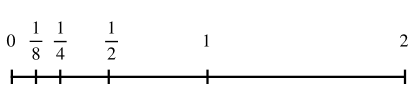
| MUTAG | PTC | ENZYMES | PROTEINS | NCI1 | IMDB-B | IMDB-M | COLLAB | |||||||||
|---|---|---|---|---|---|---|---|---|---|---|---|---|---|---|---|---|
| 82.141.2 | 65.732.4 | 62.311.4 | 78.221.6 | 80.511.2 | 63.271.1 | 50.291.4 | 70.061.3 | |||||||||
| 83.270.3 | 66.082.1 | 60.180.5 | 80.311.4 | 78.400.6 | 64.582.2 | 52.330.9 | 71.881.7 | |||||||||
| 81.731.4 | 64.811.4 | 64.461.2 | 78.310.9 | 78.221.4 | 70.842.3 | 50.421.8 | 73.491.4 | |||||||||
| 81.120.6 | 65.130.7 | 60.061.3 | 78.880.4 | 78.481.3 | 74.052.4 | 51.130.8 | 78.161.3 | |||||||||
| 82.760.9 | 65.732.4 | 64.581.7 | 79.231.2 | 80.511.2 | 70.842.3 | 51.042.2 | 74.211.2 | |||||||||
| 83.270.3 | 66.082.1 | 61.251.8 | 81.071.7 | 79.261.9 | 74.052.4 | 52.330.9 | 78.161.3 | |||||||||
| 83.270.3 | 66.082.1 | 64.461.2 | 80.311.4 | 79.141.1 | 70.842.3 | 52.330.9 | 74.541.9 | |||||||||
| 82.531.9 | 65.732.4 | 62.311.4 | 79.542.1 | 80.511.2 | 74.052.4 | 51.370.5 | 78.161.3 | |||||||||
| MUTAG | PTC | ENZYMES | PROTEINS | NCI1 | IMDB-B | IMDB-M | COLLAB | |||||||||
|---|---|---|---|---|---|---|---|---|---|---|---|---|---|---|---|---|
| 86.411.9 | 68.760.9 | 69.881.3 | 84.271.3 | 80.330.8 | 60.401.3 | 51.011.3 | 71.280.9 | |||||||||
| 84.520.8 | 67.191.2 | 66.372.1 | 81.121.7 | 77.052.2 | 62.081.6 | 52.481.0 | 72.031.2 | |||||||||
| 83.491.1 | 67.121.0 | 65.381.7 | 82.892.2 | 80.572.4 | 72.851.4 | 50.911.4 | 75.021.2 | |||||||||
| 83.341.3 | 64.220.9 | 62.240.7 | 80.030.4 | 80.901.6 | 72.491.1 | 52.080.9 | 80.892.2 | |||||||||
| 86.411.9 | 68.760.9 | 69.881.3 | 84.271.3 | 80.330.8 | 72.851.4 | 51.011.3 | 76.130.7 | |||||||||
| 84.520.8 | 67.191.2 | 67.132.2 | 82.531.1 | 80.901.6 | 72.491.1 | 53.160.8 | 80.892.2 | |||||||||
| 84.520.8 | 68.011.4 | 66.440.9 | 83.522.4 | 80.572.4 | 72.851.4 | 52.481.0 | 77.420.7 | |||||||||
| 86.411.9 | 68.760.9 | 69.881.3 | 84.271.3 | 80.901.6 | 72.491.1 | 53.481.2 | 81.121.4 | |||||||||
Our primary objective in this work is to introduce new GNNs that are equivariant to functional symmetries, based on a novel spectral domain transferable between graphs using analysis and synthesis. Our NLSFs in Sec. 3.4 consider filters that are supported on the dyadic sub-bands . The closer to the low-frequency range, the denser the sub-bands become. We illustrate an example of filters supported on dyadic sub-bands with and in Fig. 3, showing that sub-bands become denser as they approach the low-frequency range. Our primary goal is to highlight the unique aspects of our method rather than sub-band separation, which, while crucial, is an important consideration across spectral GNNs. Therefore, we also present uniform sub-bands, where filters are supported on the uniform sub-bands . Note that the modifications required for our NLSFs are minimal, and most steps can be seamlessly applied with filters supported on the uniform sub-bands.
We evaluate our NLSFs with uniform sub-bands on graph classification tasks. We consider the graph benchmarks as in Sec. 5, including five bioinformatics datasets: MUTAG, PTC, NCI1, ENZYMES, and PROTEINS, and three social network datasets: IMDB-B, IMDB-M, and COLLAB. Note the sub-bands only affect our Value-NLSFs, where Index-NLSFs remain the same as in Sec. 3.4.
We report the graph classification accuracy of Graph-NLSFs and Pooling-NLSFs using uniform sub-bands in Tab. LABEL:tab:graph_classification_nlsfp_uniform_graph_nlsf and Tab. LABEL:tab:graph_classification_nlsfp_uniform_pooling_nlsf, respectively, where the , , , and are the index-based NLSFs and therefore they are the same as in Tab. LABEL:tab:graph_classification_nlsfp_ablation_graph_nlsf and Tab. LABEL:tab:graph_classification_nlsfp_ablation_pooling. Interestingly, the Laplacian attention does not yield significant improvements for either Graph-level NLSFs or Pooling-NLSFs when considering uniform sub-bands. Moreover, we observe that the graph classification performance is generally worse than when using the dyadic sub-bands reported in Tab. LABEL:tab:graph_classification_nlsfp_ablation_graph_nlsf and Tab. LABEL:tab:graph_classification_nlsfp_ablation_pooling. We emphasize the importance of considering the spectral support of filters . Empirically, we found that using the dyadic grid is more effective, which is why we focus on it and report those results in the main paper. However, exploring other sub-bands remains an important task for future work. For instance, we plan to investigate sub-bands based on for other choices of and . In the limit when , and this “converges” to the uniform grid.