Merle Munko††*Corresponding author. Email address: merle.munko@ovgu.de, Marc Ditzhaus, Markus Pauly and Łukasz Smaga
TU Dortmund University; Dortmund (Germany)
Research Center Trustworthy Data Science and Security, UA Ruhr; Dortmund (Germany)
Adam Mickiewicz University; Poznań (Poland)
Multiple Comparison Procedures for Simultaneous Inference in Functional MANOVA
Abstract
Functional data analysis is becoming increasingly popular to study data from real-valued random functions. Nevertheless, there is a lack of multiple testing procedures for such data. These are particularly important in factorial designs to compare different groups or to infer factor effects. We propose a new class of testing procedures for arbitrary linear hypotheses in general factorial designs with functional data. Our methods allow global as well as multiple inference of both, univariate and multivariate mean functions without assuming particular error distributions nor homoscedasticity. That is, we allow for different structures of the covariance functions between groups. To this end, we use point-wise quadratic-form-type test functions that take potential heteroscedasticity into account. Taking the supremum over each test function, we define a class of local test statistics. We analyse their (joint) asymptotic behaviour and propose a resampling approach to approximate the limit distributions. The resulting global and multiple testing procedures are asymptotic valid under weak conditions and applicable in general functional MANOVA settings. We evaluate their small-sample performance in extensive simulations and finally illustrate their applicability by analysing a multivariate functional air pollution data set.
keywords:
Family-Wise Error Rate, Functional MANOVA, Functional Repeated Measures ANOVA, Heteroscedasticity, Resampling1 Introduction
Since the appearance of the notion "functional data" in the 1982 article by Ramsay (1982) and the subsequent seminal 1991 paper by Ramsay and Dalzell (1991), functional data analysis (FDA) has gained in popularity. This was already stated in the 2013 review article Ullah and Finch (2013) on applications of FDA with functional ANOVA and MANOVA among the most common inference applications (last two columns of Table 1 therein). A quick Scopus search for "functional data" highlights, that its popularity increased even more since then: counting 5,945 hits between 2014 and March 2024 compared to 4,259 hits between 1992 and 2013 as well as 318 until 1991.
In some of these papers, not only one univariate functional endpoint is of interest but a multi-dimensional vector of functions is observed for each experimental unit or individual. This is, e.g., the case with different functional endpoints or with longitudinally recorded functional data (special case of functional Repeated Measures). Examples of such data can be found in various disciplines covering longitudinal behavioural monitoring in ecology (Chiou and Müller, 2014), angular rotation curves of hip and knee through the gait cycle of children (Olshen et al., 1989), -trace measurements of different gender under longitudinal interventions (Sattler and Pauly, 2018) in medicine, functional EEG and SPECT recordings over time in different disease and control groups in neuroscience (Bathke et al., 2018) or in environmental research. An example of the latter are given by the Canadian weather data set available in the R package fda (Ramsay et al., 2022), where daily temperature and precipitation is collected or the data set on air pollution in the U.S. analyzed in Zhu et al. (2022), in which the trajectories of three pollutants were recorded over a year. In all these examples, a longitudinal or multivariate functional design is present and the comparison of different groups or experimental conditions over time is of interest. Thus, we need multivariate analysis of variance (MANOVA) methods that can test global (e.g., about group, factor, time or interaction effects) as well as multiple linear hypotheses of mean functions (e.g. all-pairs, many-to-one or factorial change points) in arbitrary factorial designs covering crossed as well as functional Repeated Measures ANOVA (i.e. longitudinal).
There exist various global testing procedures for univariate functional data, see, e.g. Cuevas et al. (2004); Górecki and Smaga (2015); Paparoditis and Sapatinas (2016); Pomann et al. (2016); Liebl and Reimherr (2023) or the monograph by Zhang (2013) on functional ANOVA. In comparison, functional MANOVA seems to be less researched in the literature until recently. Cao and Wang (2018); Smaga (2020); Wang et al. (2020) proposed inference procedures in case of functional Repeated Measures ANOVA with one or two groups. More general, Górecki and Smaga (2017) studied permutation tests based on a basis function representation and on random projections for the multivariate analysis of variance (MANOVA) problem for homoscedastic functional data, i.e., functional data with the same covariance structure between the groups. Qiu et al. (2021) proposed two global tests for multivariate homoscedastic functional data in the two-sample case by integrating the pointwise Hotelling‘s -test statistic and taking its supremum, respectively. Moreover, Zhu et al. (2022) developed another global test for the MANOVA problem for potentially more than two samples by using the functional Lawley–Hotelling trace test statistic still assuming homoscedasticity. Homoscedasticity is already a very restrictive assumption in classical ANOVA (e.g. Pauly et al., 2015) and is rarely fulfilled in real applications with multivariate functional data. Some solutions that allow for heteroscedasticity have been published recently for the one-way functional MANOVA setting by Zhu et al. (2022, 2024). Moreover, extensions to general linear hypotheses can be found in the preprint Zhu (2024). The lack of approaches for multiple testing of mean functions is even more serious. There only exist a recent preprint for the univariate case by the authors (Munko et al., 2023). However, there exist no multiple testing procedures for general functional MANOVA (covering functional Repeated Measure ANOVA as special case) to the best of our knowledge.
Thus, it is the aim of the present paper to develop a new class of global and multiple testing procedures for general linear hypotheses in the functional MANOVA context. The procedures do not postulate heteroscedasticity nor a specific distribution and can be flexibly applied to all kind of multivariate factorial designs covering one-way, crossed two-way or general longitudinal and split-plot settings with functional data. To this end, we consider Wald-type test statistics for global hypotheses which take the heteroscedastic nature of the functional data into account. Since their limit distributions turn out to be rather complicated, we adapt the parametric bootstrap approach of Cuevas et al. (2004) to the present setting to approximate the limit distribution and prove its asymptotic correctness. To also allow for general multiple comparisons with family-wise error rate control, the asymptotic exact dependence structure of the test statistics is incorporated to determine suitable critical values that lead to valid test decisions.
The remainder of this paper is organised as follows. Section 2 is divided into four subsections. The general setup of the linear hypothesis testing problem for multivariate heteroscedastic functional data is presented in Section 2.1. A suitable test statistic for this testing problem is proposed and studied in Section 2.3. In Section 2.4, the parametric bootstrap procedure is extended to multivariate functional data. Furthermore, we construct multiple tests in Section 2.5 for testing multiple hypotheses. In addition, the finite sample performance of the proposed tests is analysed in intensive simulation studies in terms of size control and power in Section 3. In Section 4, our proposed methodologies are applied to a data example. Finally, the results of this paper are discussed in Section 5. The proofs of all theorems and auxiliary technical results are given in the supplement.
2 Statistical Methodology
In this section, we introduce the general functional set-up, a suitable test statistic for the global testing problem and the parametric bootstrap approach for constructing global testing procedures for general linear combinations of multivariate mean functions. Moreover, we develop multiple testing procedures and state the asymptotic validity of all procedures.
2.1 General Functional Set-Up
Throughout this paper, let denote a compact pseudometric space, e.g., with the Euclidean metric. We write and for a -dimensional Gaussian or general stochastic process , respectively, over with mean function , covariance function and . Suppose we have independent multivariate functional samples given by -dimensional stochastic processes
| (1) |
with sample sizes and dimension .
Here, denotes the multivariate mean function and denotes the covariance function of the th sample for all , which are both unknown.
The total sample size is denoted by .
In contrast to the multivariate set-ups considered in Górecki and Smaga (2017, p. 2173), Qiu et al. (2021) or Zhu et al. (2022), the covariance functions may differ from each other, i.e. we are not assuming homoscedasticity.
To infer general linear hypothesis about the mean functions, let denote a known matrix with . Furthermore, let be the vector of all mean functions and be a fixed function. In many settings, we use the zero function for all . In the following, we consider the null and alternative hypothesis
| (2) |
We note, that this generalizes the setting of Zhu (2024) who considered hypotheses of the form for a matrix which can be rewritten in our formulation with and for all . We additionally stress, that this set-up is very flexible. In particular, it allows for a factorial structure within the pooled vector of mean functions by splitting up indices as in classical ANOVA or MANOVA (Konietschke et al., 2015; Pauly et al., 2015) and thus covers all kind of hypotheses in general factorial designs with functional data. Specific examples are given by one- or crossed two-way univariate and multivariate functional analysis of variance problems as well as longitudinal settings as outlined below.
Example 2.1.
-
(a)
One-Way fMANOVA: For the one-way functional MANOVA, we may choose for all and , where here and throughout denotes the unit matrix and is the matrix of ones. This results in the null hypothesis for all .
-
(b)
Crossed Two-Way fMANOVA: In a functional two-way design with factors A with levels and B with levels, we set and split up the group index in two subindices . Thus, the following null hypotheses are covered by our formulation of the testing problem:
-
•
No main effect of factor A: for all ,
-
•
No main effect of factor B: for all ,
-
•
No interaction effect between factors A and B: for all .
-
•
-
(c)
Longitudinal fANOVA: For the one-way Repeated Measures fANOVA, we set , where denotes the number of repeated measures and denotes the dimension. Hence, corresponds to the mean function of an individual in group measured at and . Then, the following hypotheses can be formulated in our testing framework:
-
•
No group effect: for all ,
-
•
No time effect: for all ,
-
•
No interaction effect between time and group: for all .
-
•
-
(d)
Testing for specific functional pattern: If it is of interest whether the vector of mean functions has a specific functional pattern , we can choose as unit matrix and, thus, receive the null hypothesis for all .
2.2 General Assumptions
In the following, we consider the space of -dimensional continuous functions . For constructing suitable tests for the general testing problem (2) and analyzing their asymptotic properties, the following assumptions are required.
Assumption 2.2.
Consider the independent samples (1). Let denote the subject-effect functions. Additionally, assume that the following conditions (A1)–(A5) are fulfilled for all
-
(A1)
The subject-effect functions are i.i.d. and take values in .
-
(A2)
There exists a such that , where here and throughout denotes the 2-norm of a vector.
-
(A3)
The covariance matrix is positive definite for all .
-
(A4)
There exists a such that as .
- (A5)
Assumptions (A1)–(A4) are standard assumptions in the functional data setup in the space of continuous functions, see e.g. Dette et al. (2020). Assumptions (A1), (A4) and (A5) will guarantee the asymptotic Gaussianity of the mean function estimators and the parametric bootstrap counterparts. Assumptions (A1), (A2) and (A5) will yield the uniform consistency of the covariance function estimators and the parametric bootstrap counterparts. From this, the convergence of our proposed test statistic will follow by using (A3).
Assumption (A5) is motivated by (A3) in Dette et al. (2020) but less restrictive since we replaced it by a moment condition.
Moreover, Dette et al. (2020) focused on with the metric and while we allow general pseudometric spaces .
However, for and , (3) is fulfilled whenever and, thus, the restrictions on are slightly stronger than in their paper.
Condition (3) results from empirical process theory (van der Vaart and Wellner, 1996, Theorem 2.2.4) and is required with a higher order than in Dette et al. (2020) since the parametric bootstrap estimators of the covariance functions are incorporated in our test statistic (8), see the proof of Lemma S8 in the supplement for details.
2.3 Globalising Pointwise Hotelling’s -Test Statistic
In this section, we present a suitable test statistic for the testing problem (2). Therefore, we use a similar test function as in Munko et al. (2023). However, we globalise this test function by taking the supremum instead of integrating over it since the supremum seemed to outperform the integral in our simulation studies. For constructing the test function, we firstly define an unbiased estimator for the mean function of the th group at by
and for the covariance function of the th group at by
| (4) |
for all . By the weak law of large numbers, the mean function estimators and covariance function estimators are pointwisely consistent under (A1).
Furthermore, we show that the covariance function estimators are uniformly consistent over
under (A1), (A2) and (A5) in Lemma S6 in Section S1 in the supplement.
Let
be an estimator for
for all , where denotes the direct sum of the matrices . It should be noted that is invertible under (A3) and (A4) for all . The pointwise consistency of the covariance function estimators provides immediately the pointwise consistency of under (A1) and (A4).
Moreover, the uniform consistency of over is proven in Lemma S6 under the assumptions (A1), (A2), (A4) and (A5).
Then, a reasonable point-wise test statistic for the multivariate functional data setup is defined by
| (5) |
for all , where denotes the vector of all mean function estimators.
Following Qiu et al. (2021) we call the point-wise Hotelling’s -test statistic. We expect that the point-wise Hotelling’s -test statistic is small for all under the null hypothesis in (2) since is an estimator for . Moreover, can be viewed as an approximation of the covariance matrix of .
Based on the point-wise Hotelling’s -test statistic (5), we can construct a test statistic by taking the supremum over the point-wise test statistics, that is
| (6) |
The null hypothesis in (2) shall be rejected for large values of the test statistic.
Similarly to the invariance properties of the GPH statistic for the univariate functional data setup in Munko et al. (2023), one can show the invariance under orthogonal transformations, i.e., for any orthogonal , and the scale-invariance in the sense of Guo et al. (2019) for the multivariate case.
For the construction of asymptotic tests based on the proposed test statistic, we have to examine its asymptotic behaviour. The limiting distribution of the test statistic under the null hypothesis is given by the following theorem.
Theorem 2.3.
The limiting distribution depends on the unknown covariance functions and is thus non-pivotal. To overcome this issue, we below propose a resampling approach to compute adequate critical values.
2.4 Parametric Bootstrap
In this section, we adopt a parametric bootstrap approach as proposed in Munko et al. (2023) to the present set-up.
Note that a similar bootstrap approach has been proposed earlier by Dette et al. (2020) in the case of univariate functional time series.
In this method we substitute by their estimators. Then, the parametric bootstrap samples are given by conditionally on the functional data .
Note, that we still postulate our general model, i.e., we do not assume a parametric model for our functional data . The idea, however, is that the bootstrap samples reflect the dependency structure of the true processes; where the distribution is motivated by the functional CLT.
In the following, we denote the parametric bootstrap counterparts of the statistics defined in Section 2.3 with a superscript
Thus, we define the parametric bootstrap pointwise Hotelling’s -test statistic at by
for all Taking the supremum yields the parametric bootstrap globalising pointwise Hotelling‘s -test statistic for the multivariate functional data setup, that is
| (8) |
The consistency of the proposed parametric bootstrap is stated in the following theorem.
Thus, the parametric bootstrap test statistic always mimics the distributional limit of given in (7). The distribution of is usually approximated by Monte Carlo with iterations. Thus, we obtain the parametric bootstrap test
where here and throughout denotes the level of significance. Moreover, denotes the empirical -quantile of , where are independent copies of conditionally on the data . It follows that is an asymptotic level- test for large and large .
Proposition 2.5.
Remark 2.6.
Our proposed test is a very flexible tool for inferring different global linear hypotheses of the mean functions of different groups in a general heteroscedastic multivariate functional setting. In the next subsection, we propose extensions for multiple testing that particularly allow for post-hoc testing.
2.5 Multiple Tests
In many applications, it is not only of interest whether there exists a (global) significance but also which specific linear combinations cause the significance. For example, hypotheses about pairwise comparisons often contain the main research questions in one-way layouts. Hence, general multiple tests for heteroscedastic functional data are needed and constructed in this section. To this end, we use the same strategy as in the univariate case (Munko et al., 2023) for constructing multiple tests with consonant and coherent test decisions as defined in Gabriel (1969). Therefore, the exact asymptotic dependence structure of the local test statistics is taken into account. In Munko et al. (2023), simulations have already shown that this procedure yields to a high power and quite accurate family-wise error control for univariate functional data.
In the following, we interpret as a block matrix, that is for matrices with , and as function with component functions for all , where such that . Note that we do not restrict to but also cover the case that is partitioned in row vectors . The main idea of multiple tests is to split up the global null hypothesis in (2) with hypothesis matrix and function into single tests with hypothesis matrices and functions , respectively. This leads to the multiple testing problem
| (12) |
Again, this formulation covers many special cases as will be pointed out in the following example.
Example 2.7.
In this example, we focus on all-pairs comparisons and many-to-one comparisons of the mean functions. Further suitable hypothesis matrices, e.g. for trend, can be found in Bretz et al. (2001).
-
(a)
All-Pairs Comparisons: Pairwise comparisons of the mean functions can be considered by choosing as the Kronecker products of the rows of the Tukey-type contrast matrix (Tukey, 1953) and the unit matrix and for all . This yields the multiple hypotheses for all with .
-
(b)
Many-To-One Comparisons: When there is a reference group, it makes sense to compare the mean functions of all other groups to this reference group. Here, we assume that the first group is the reference group. Thus, we are interested in the hypotheses for all with We obtain these hypotheses by choosing for all and for all , where denotes the transposed th unit vector. Here, the row vectors are the rows of the Dunnett-type contrast matrix (Dunnett, 1955).
To derive a valid multiple testing procedure, we first investigate the joint distribution of the local test statistics in more detail.
Theorem 2.8.
As in the global testing case, the limit distribution is non-pivotal. But even in this case, the vector of the parametric bootstrap counterparts mimic the limit as shown below.
The theorem can be used to derive a consistent parametric bootstrap procedure for the multiple testing problem. To this end, draw independent copies of conditionally on the data given by
for some sufficiently large . Denote the empirical -quantile of for all as . Then we define a new class of multiple parametric bootstrap tests by
Here, is chosen such that the approximated family-wise error rate is bounded by the level of significance , see Section 3 in Munko et al. (2024) for details. Each test statistic is treated in the same way and has the same impact since we use the same local level for each linear combination. The following proposition ensures that the proposed multiple testing procedure asymptotically controls the family-wise error rate.
Proposition 2.10.
As in Remark 2.6, it also holds that
3 Simulations
In this section, we investigate the finite sample properties of the new tests and their competitors. We consider the control of the type I error level, power and scale-invariance of the tests.
The new global parametric bootstrap test of Section 2.4 will be denoted by SPH (supremum of the pointwise Hotelling’s -test statistic). On the other hand, the mSPH test is the new multiple parametric bootstrap test (see Section 2.5). We consider the following competitors for our new tests (see also Section 1):
-
(a)
W, LH, P, R (Górecki and Smaga, 2017) - the permutation tests based on a basis function representation of functional data and the Wilks’, Lowley-Hotelling’s, Pillay’s, and Roy’s test statistics, respectively,
-
(b)
Wg, LHg, Pg, Rg (Górecki and Smaga, 2017) - the tests based on random projections of functional data using gaussian white noise and the Wilks’, Lowley-Hotelling’s, Pillay’s, and Roy’s test statistics, respectively,
-
(c)
Wb, LHb, Pb, Rb (Górecki and Smaga, 2017) - the tests based on random projections of functional data using Brownian motion and the Wilks’, Lowley-Hotelling’s, Pillay’s, and Roy’s test statistics, respectively,
-
(d)
ZN, ZB (Zhu et al., 2024) - the tests for MANOVA problem for heteroscedastic functional data based on naive and bias-reduced estimators, respectively,
-
(e)
Z (Zhu, 2024) - the test for general linear hypotheses testing problem for heteroscedastic functional data,
- (f)
-
(g)
QI, QS (Qiu et al., 2021) - the two-sample tests based on integrating and taking supremum of the pointwise Hotelling’s -test statistic, respectively. They are used just in the scenario of two-samples for which they are designed.
When we use the global tests (i.e., the test other than mGPH and mSPH) for the multiple testing problem, the Bonferroni correction is used. Note that the tests QI, QS, W, LH, P, R, Wg, LHg, Pg, Rg, Wb, LHb, Pb, and Rb are constructed for homoscedastic functional data.
3.1 Simulation setup
Qiu et al. (2021) already conducted a simulation study for the case with two independent groups. For a fair comparability with existing methods, we inspire our models from their study. For ease of presentation, we thereby focus on one-way designs.
Model 1. We first consider a one-way layout with groups and functional variables. Following (Qiu et al., 2021, Simulation 2), we consider the following linear functional model:
Below we discuss the different choices for this set-up.
Mean Functions. The vectors , , of mean functions in the first three samples are constructed as follows:
In the last sample, we take for , and
| (14) |
When the hyperparameter , the null hypothesis is true, while if , the alternative holds and controls the difference between the mean functions. We specify its values below.
Covariance Functions. We set , where
and , , , and , , , for . We let with the following three scenarios of : . The homoscedastic case is represented by , while and correspond to two heteroscedastic scenarios. Set sample sizes to , and . Then, for the heteroscedastic cases, we have the positive and negative pairings scenarios for and , respectively, i.e., the variability increases and decreases, respectively, while sample sizes increase (see, for example, Pauly et al., 2015). As we will see in simulation results, it has an impact on the properties of many of tests considered. The parameter corresponds to the correlation in functional data, namely, the smaller the larger correlation. We set . Since the power of the tests depends on the amount of correlation in the data, we consider for , respectively, to usually obtain a non-trivial power of the tests.
Error Distributions. The random variables are generated independently from three standard distributions: , , and . They represent symmetric and skewed distributions as well as the light-tailed and heavy-tailed ones.
Scaling. We would also check the impact of scaling functional data on the properties of the tests (see Section 2.3). Thus, in addition to the above scenario without scaling function, we also consider the case of scaling generated functional observations by the function for . Note that the tests QI, QS, ZN, ZB, Z, GPH, mGPH, SPH, and mSPH are scale-invariant, while the tests by Górecki and Smaga (2017) are not.
Studied Hypotheses. For global and multiple testing problem, we consider the Tukey-type contrast (Tukey, 1953). Thus, we compare each pair of different groups (each pair just one time), i.e., for , we have six contrasts 1-2, 1-3, 1-4, 2-3, 2-4, and 3-4. Then, the hypothesis matrix for testing the global hypothesis for all in (2) is given by
For the multiple testing problem, we split this matrix into a block matrix , where and is the -th row of , . This corresponds to the individual hypotheses for all and .
Model 2. To compare the new test with the two-sample tests by Qiu et al. (2021), we also consider the two-sample problem with and . The simulation setup is the same as in Simulation 1 in Qiu et al. (2021), and it is very similar to that presented above. Let us just point out the differences. The mean functions are , , and is the same as given in (14). The variability is controlled by the vectors: , , and . The sample sizes are , and
The functional observations are discreetly observed in so-called design time points. Here, their values are calculated in 50 equally spaced points in the interval . The examples of trajectories of generated functional data in simulation study are presented in Figures S1-S3 in the supplement.
Evaluation Criteria and Simulation Runs. We evaluated the global hypothesis tests by means of their size (type I error rate) and power. To obtain reliable estimates, the empirical size and power of each test is calculated as the proportion of rejections in 1000 repetitions of simulation under the null (size) and alternative hypothesis (power), respectively.
For the multiple testing procedures, we use the family-wise error rate (FWER) and the local power for evaluation. The empirical FWER is computed as the proportion of rejecting at least one true null hypothesis. Moreover, the empirical local power is calculated in the same way as for the global hypothesis, but separately for each non true hypothesis.
For the resampling tests, the number of bootstrap or permutation samples equals 1000. The significance level is set to . The simulation experiments were conducted in the R programming language (R Core Team, 2023). The R code for all numerical experiments is given in the supplement.
3.2 Simulation results
In this section we discuss our findings in detail by means of the four summarizing Figures 1-4. Additional details on all simulation results are presented in separate tables and figures in the supplement (Tables S1-S10, Figures S4-S13). Figures 1, 3 and 4 show the properties of the tests for homoscedastic and both heteroscedastic cases under different scenarios. On the other hand, Figure 2 presents the effect of different amounts of correlation in the functional data. We note that we throughout excluded the Rg and Rb tests for ease of presentation as they were extremely liberal in all cases (confer Tables S1 and S5 in the supplement).
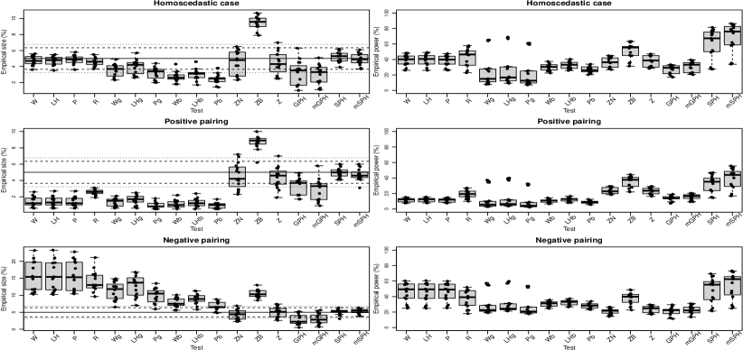
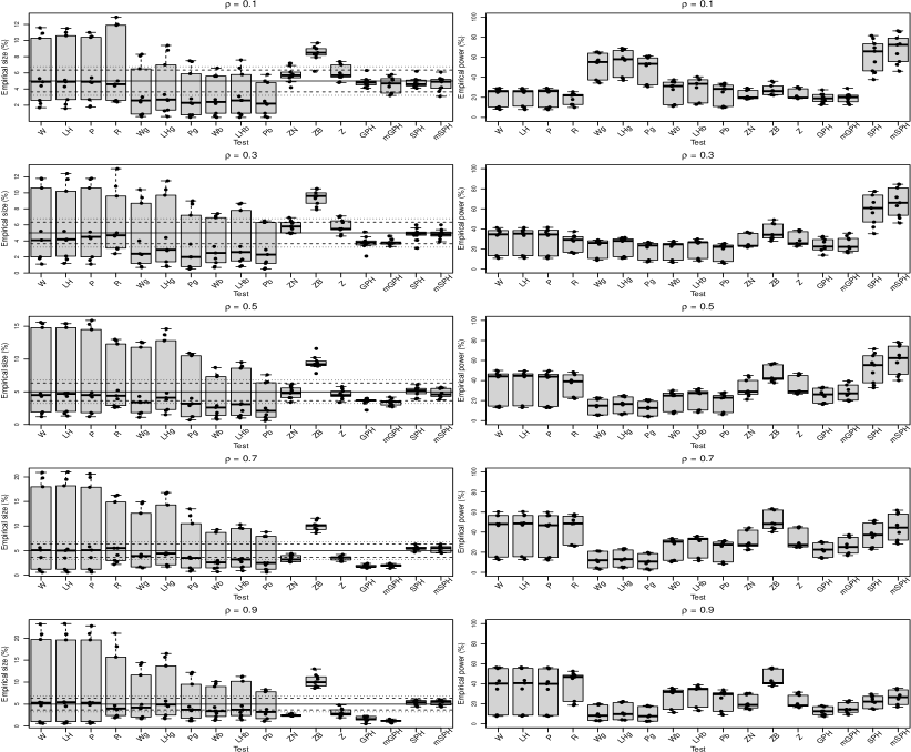
Global Hypothesis Testing. The results for testing the global hypothesis for all are given in Figures 1-2. The mGPH and GPH tests (third and fourth from last boxplot in each plot) by Munko et al. (2023) worked well for one-dimensional functional data. However, for our multivariate settings, they exhibit a rather conservative character (left plots, median empirical sizes always below 5%), especially for larger negative pairing (last row of Figure 1) or larger correlations (last rows of Figure 2). This resulted in smaller power (right plots). The ZB test (six last boxplot) is always too liberal. The two other tests of this type, ZN and Z (fifth and seventh last boxplots), control the type I error level much better, but are sometimes a bit too conservative or too liberal (whiskers and parts of boxes outside the binomial interval). On the other hand, both mSPH and SPH tests (last and second last boxplot in each plot) control the type I error level very well, being neither conservative nor liberal. In fact, these are the only two methods that control type I error level independently of variance pairing or correlations. For describing the results of the remaining ten procedures, we therefore distinguish the settings. Under homoscedasticity (first row of Figure 1), the permutation W, LH, P, and R tests control the type I error level well. The other projection tests, i.e. the Wg, LHg, Pg, Wb, LHb, and Pb tests, exhibit a conservative character which is common for this type of test, see, e.g. Górecki and Smaga, 2017. Under positive pairing, all of these ten tests are conservative, while for negative pairing, they are too liberal. Regarding power, the most accurate procedures, SPH and mSPH, are usually also the most powerful, except for the cases with larger correlations (Figure 2 with and to some extend also ). However, in this case, the new tests are comparable with other tests and control the type I error level well in contrast to most of the competitors. Moreover, the mSPH test is usually better than the SPH test, which shows the improvement of using the multiple testing procedure proposed in Section 2.5 compared to naive Bonferroni. The GPH and mGPH tests are usually much less powerful. In comparison with the other competitors, they are sometimes slightly better, comparable, or worse. However, the GPH and mGPH tests are never too liberal, which is not true for the competitors.
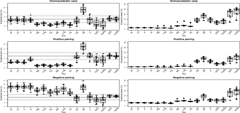
Impact of Scaling. Let us now discuss the impact of scaling functional data on the properties of the global testing procedures. The results are given in Figure 3. The new tests and the GPH, mGPH, ZN, ZB, and Z tests are scale-invariant. Thus, the simulation results are similar to the cases without scaling. On the other hand, the tests by Górecki and Smaga (2017) (first ten boxplots in all plots) are not scale-invariant, and their empirical power for the present case with scaling is much smaller than for the without scaling case. In fact, they often do not exhibit any power at all for the scaled alternatives.
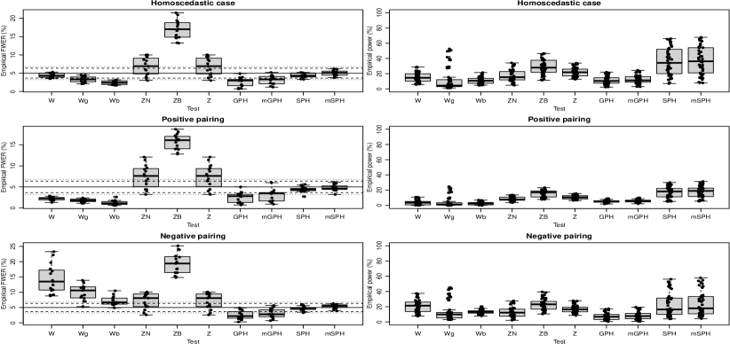
Multiple Testing. Turning to the multiple testing problem, Figure 4 shows the empirical family-wise error rate (FWER) and power (as percentages) of the studied procedures. For ease of presentation, we only present the results for the W, Wg, and Wb tests by Górecki and Smaga (2017) using the Wilks test statistic, since these tests are the best representation of that kind of testing procedure. In general, the conclusions are similar to the above ones for testing the global hypothesis. In fact, the new mSPH and SPH tests (last and second to last boxplots) exhibit the best results in terms of FWER control and power. However, note that the global SPH test with Bonferroni correction is at least slightly more conservative than the mSPH test. Moreover, the ZN, ZB, and Z tests do not control the FWER correctly in many cases, i.e., they are mainly too liberal.
The Classy Two-Sample Problem. Two-sample comparisons are among the most relevant. That is why we finally study the suitability of the new method for the two-sample testing problem. The detailed results are given in Section S1.4 in the supplement and we only summarize our findings here. Again, the conclusions for all previously considered tests are similar. However, we additionally compare with the recently proposed two sample methods QI and QS by Qiu et al. (2021) and thus elaborate on them a bit. In many cases, the QI test is too liberal, especially for negative pairing but also for the homoscedastic case. Nevertheless, it is less powerful than the QS test in almost all settings. The QS test is too liberal in negative pairing but otherwise controls type I error level quite well. In contrast, the new SPH test shows the best type I error level control. Moreover, the QS and SPH tests are usually the most powerful, but QS is at least slightly less powerful than SPH.
To sum up, in contrast to the competitors, the new SPH and mSPH tests control the type I error level in all scenarios and usually have the best power. From these two tests, the mSPH test using the multiple testing procedure from Section 2.5 is at least slightly better than the global SPH test with Bonferroni correction.
4 Illustrative Data Analysis
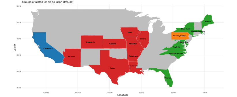
In this section, we illustrate the application on a real data example. It is based on the U.S. air pollution data which is available from https://www.kaggle.com/datasets/sogun3/uspollution and was also studied in Zhu et al. (2022). It contains daily concentration measurements of four major pollutants, namely, Nitrogen Dioxide (NO2), Ozone (O3), Sulfur Dioxide (SO2), and Carbon Monoxide (CO) in U.S. cities for many years. For illustrative purposes, we only consider the period from 31 March to 31 October 2008. We used the data for the 2008 year since there are quite a lot of observations for cities in California and Pennsylvania. Moreover, we did not take a whole year, since at its beginning and end, there were a lot of missing values, especially for cities in Pennsylvania. After removing missing values and outliers (detected by visual inspection, see the R code in the supplement for details), we consider the following four samples:
-
(1)
13 functional observations for cities in California,
-
(2)
15 functional observations for cities in Pennsylvania,
-
(3)
9 functional observations for cities in the East states in the USA,
-
(4)
15 functional observations for cities in the Central states in the USA.
The groups of states are presented in Figure 5. Pennsylvania is also located in the eastern part of the USA, but we excluded it from the East states category. The reason for this is that we have data for many cities in Pennsylvania, while for other states, there are data for only one or two cities. As in Zhu et al. (2022), each daily concentration measurement raw curve was first smoothed using a B-spline basis of order 4 and with 20 basis functions. Then, the resulting smoothed concentration measure curve was evaluated over a common grid of time points (215 is the number of days between 31 March to 31 October).


From the four major pollutants, the SO2 variable is very different in the four groups. As this would result in rejecting the null hypothesis by all testing procedures, we omit for our illustrative analysis. Thus, each functional observation in this example is a three-dimensional vector of functions corresponding to three pollutants NO2, O3, and CO. The trajectories of our multivariate functional data are presented in Figure 6. We are interested in comparing the ’location’ of the four groups. In particular, we want to test the equality of vectors of group-wise mean functions. The sample mean functions are presented in Figure 7 (see also Figure S14 in the supplement). They suggest that there are some differences between the four regional groups. To infer this, we applied all tests considered in Section 3. The results for the global hypotheses are presented in Table S12 in the supplement while Table 1 shows the results for the six local hypotheses (the columns in both tables).
In addition, to this illustrative analysis we also conducted a Plasmode-type study, i.e. a simulation study that mimics the present set-up. This allows us to better assess the trustworthiness of the tests’ results. To this end, we simulated four groups with the same sample sizes , , , and from Gaussian processes with group-wise covariance functions equal to the sample covariance functions estimated from the data. Moreover, as group-wise mean functions we used (a) the vector of sample mean functions to asses power (’Power’ column in the tables) or (b) the pooled sample mean function to infer type-I-error control (’FWER’ in Table 1 and ’Size’ in Table S12). All tests reject the global null hypothesis and their empirical power is close to (Table S12 in the supplement). However, most tests are too liberal with empirical sizes up to (e.g. for Rg) instead of the desired . In fact, only the Pb test and the four PH-tests (GPH, mGPH, SPH and mSPH) exhibit type I error levels smaller than (Table S12 in the supplement). The bad properties of some of the tests can be explained by the significant differences in covariance functions in these four groups, which is suggested by the tests for equality of covariance functions for one-dimensional functional data applied to each functional variable separately (see Section S2.1 in the supplement for more details). Nevertheless, it seems that the vectors of mean functions of the three pollutants are significantly different in the four groups.
As we rejected this global hypothesis, we conducted a post-hoc analysis (Table 1) to find out which groups are significantly different and which are not. We can observe that all tests reject the equality for cities in California and Pennsylvania as well as in Pennsylvania and the Central states. On the other hand, in the comparison ’Pennsylvania vs. East states’, no test rejects the null hypothesis, which is perhaps caused by the geographical similarity. Finally, we comment the remaining pairs, which are the most interesting cases. Here, we can observe large differences between the methods. Most tests do not reject the null hypotheses which also matches their lower power in the mimicking simulation study. On the other hand, the new SPH (except for the case ’California vs. East states’) and mSPH tests as well as the Wg test reject the local null hypotheses and also have larger power in the corresponding simulation study. However, note that the Wg test is a bit too liberal (estimated FWER of 7.3%) in the mimicking simulation study, perhaps due to the heteroscedastic character of the data. Thus, the most trustworthy results are obtained from the SPH and mSPH tests. Moreover, similar to Section 3, we also observe a better performance of the mGPH and mSPH tests than the GPH and SPH tests in this simulation study.
5 Discussion
We have proposed a novel class of inference methods for testing (i) global and (ii) local hypotheses about general linear combinations of multivariate mean functions in a functional MANOVA setting. While some methods for (i) were already known (though most under quite restrictive assumptions), we are the first to establish multiple testing procedures with family-wise error rate (FWER) control for (ii) (except for simple Bonferroni adjustments). We have proven the asymptotic validity of the novel procedures under weak assumptions, neither requiring Gaussianity nor homoscedasticity, i.e. we do not need to assume equal covariance functions across groups. Moreover, the proposed methods are even scale invariant. To facilitate their application, all new statistical tests are implemented in the R package gmtFD, which will appear on CRAN soon.
In a comparative simulation study it turned out that both, the new global and multiple testing procedures exhibit accurate type I error rate and FWER control, respectively. In particular, while most existing approaches were either too conservative or too liberal depending on whether positive or negative pairing was present, the new approaches turned out to be robust with respect to changes of covariance functions, dependence structure or sample sizes. In addition, the new methods were also shown to be preferable in terms of power in most studied settings. A reason for this may lie in the form of our test statistics which are based upon globalising pointwise Hotelling--type statistics via the supremum. We note that it would also be possible to globalise by integrating over it. In fact, our derived theory would in principle also work for this case. However, initial simulation results with regard to the procedures’ power were not as convincing as for the supremum-statistic.
The proposed methods are valid for general factorial designs covering crossed or non-crossed one-, two- and higher-way designs as well as nested layouts. Moreover, they are applicable with multivariate functional data, longitudinal functional data and even longitudinal multivariate functional data. Hence, many special cases, like the functional MANOVA or functional Repetated Measures ANOVA problem are covered. As the current paper focused on the thorough methodological development of the procedures, we could only exemplify the practicability for some special designs. A detailed study of the methods’ applicability and numerical performance for other important designs, such as one and two group Repeated Measures or complex Split Plot designs, will be done in future research.
| California vs. | California vs. | California vs. | Pennsylvania vs. | Pennsylvania vs. | East states vs. | |||||||||||||
|---|---|---|---|---|---|---|---|---|---|---|---|---|---|---|---|---|---|---|
| Pennsylvania | East states | Central states | East states | Central states | Central states | |||||||||||||
| Test | FWER | Power | Power | Power | Power | Power | Power | |||||||||||
| W | 8.3 | 0.6 | 98.4 | 89.4 | 19.2 | 45.6 | 39.2 | 100.0 | 19.8 | 0.6 | 97.4 | 100.0 | 15.3 | |||||
| Wg | 7.3 | 0.0 | 100.0 | 0.6 | 99.5 | 0.2 | 98.6 | 100.0 | 44.3 | 0.0 | 100.0 | 2.2 | 71.0 | |||||
| Wb | 5.0 | 0.0 | 99.1 | 19.6 | 75.3 | 75.7 | 31.2 | 100.0 | 19.6 | 0.0 | 98.8 | 87.8 | 27.3 | |||||
| ZN | 12.4 | 0.0 | 98.9 | 55.2 | 50.6 | 52.4 | 50.8 | 100.0 | 22.8 | 0.0 | 100.0 | 100.0 | 36.5 | |||||
| ZB | 19.2 | 0.0 | 99.8 | 35.6 | 67.1 | 34.8 | 64.0 | 100.0 | 37.7 | 0.0 | 100.0 | 75.1 | 60.8 | |||||
| Z | 9.5 | 0.1 | 98.0 | 27.5 | 48.8 | 44.4 | 43.2 | 100.0 | 19.5 | 0.0 | 100.0 | 63.1 | 36.1 | |||||
| GPH | 4.7 | 1.2 | 90.8 | 57.6 | 26.9 | 75.0 | 25.4 | 100.0 | 8.0 | 0.0 | 99.6 | 100.0 | 14.9 | |||||
| mGPH | 5.8 | 1.1 | 93.1 | 33.0 | 32.4 | 40.9 | 30.8 | 91.9 | 8.9 | 0.0 | 99.8 | 61.5 | 18.7 | |||||
| SPH | 5.0 | 0.0 | 99.6 | 5.4 | 77.6 | 4.8 | 87.5 | 100.0 | 19.1 | 0.0 | 100.0 | 0.0 | 99.8 | |||||
| mSPH | 5.7 | 0.0 | 99.8 | 4.5 | 81.2 | 4.1 | 89.9 | 71.6 | 22.2 | 0.0 | 100.0 | 0.0 | 99.8 | |||||
Appendix A Remarks on Assumption 2.2
In this section, we state remarks about Assumption 2.2. Here, we see that various other properties follow from these assumptions.
- (R1)
- (R2)
- (R3)
Competing interests
No competing interest is declared.
Data Availability Statement
The data underlying this article are available in the article and in its online supplementary material, there is the R code for preparing the data set.
Acknowledgments
The authors are grateful to Prof. Tianming Zhu for sharing us the code for Zhu (2024) and Zhu et al. (2024). Merle Munko and Marc Ditzhaus gratefully acknowledge funding by the Deutsche Forschungsgemeinschaft (DFG, German Research Foundation) - 314838170, GRK 2297 MathCoRe. A part of calculations for the simulation study and real data example was made at the Poznań Supercomputing and Networking Center (grants 382 and pl0253-02).
Supplementary materials
The supplement contains all proofs, all results of simulation studies of Section 3, more details about the analysis of real data examples of Section 4 of the main paper, and the R code for all numerical experiments.
References
- Bathke et al. (2018) A. C. Bathke, S. Friedrich, M. Pauly, F. Konietschke, W. Staffen, N. Strobl, and Y. Höller. Testing mean differences among groups: multivariate and repeated measures analysis with minimal assumptions. Multivariate Behavioral Research, 53(3):348–359, 2018.
- Bretz et al. (2001) F. Bretz, A. Genz, and L. A. Hothorn. On the numerical availability of multiple comparison procedures. Biometrical Journal, 43(5):645–656, 2001.
- Cao and Wang (2018) G. Cao and L. Wang. Simultaneous inference for the mean of repeated functional data. Journal of Multivariate Analysis, 165:279–295, 2018.
- Chiou and Müller (2014) J.-M. Chiou and H.-G. Müller. Linear manifold modelling of multivariate functional data. Journal of the Royal Statistical Society Series B: Statistical Methodology, 76(3):605–626, 2014.
- Cuevas et al. (2004) A. Cuevas, M. Febrero, and R. Fraiman. An ANOVA test for functional data. Computational Statistics & Data Analysis, 47(1):111–122, 2004.
- Dette et al. (2020) H. Dette, K. Kokot, and A. Aue. Functional data analysis in the Banach space of continuous functions. The Annals of Statistics, 48(2):1168 – 1192, 2020.
- Duchesne and Francq (2015) P. Duchesne and C. Francq. Multivariate hypothesis testing using generalized and -inverses - with applications. Statistics, 49:475–496, 2015.
- Dunnett (1955) C. W. Dunnett. A multiple comparison procedure for comparing several treatments with a control. Journal of the American Statistical Association, 50(272):1096–1121, 1955.
- Gabriel (1969) K. R. Gabriel. Simultaneous test procedures–some theory of multiple comparisons. The Annals of Mathematical Statistics, 40(1):224–250, 1969.
- Górecki and Smaga (2015) T. Górecki and Ł. Smaga. A comparison of tests for the one-way anova problem for functional data. Computational Statistics, 30:987–1010, 2015.
- Górecki and Smaga (2017) T. Górecki and Ł. Smaga. Multivariate analysis of variance for functional data. Journal of Applied Statistics, 44(12):2172–2189, 2017.
- Guo et al. (2019) J. Guo, B. Zhou, and J. Zhang. New tests for equality of several covariance functions for functional data. Journal of the American Statistical Association, 114:1251–1263, 2019.
- Konietschke et al. (2015) F. Konietschke, A. C. Bathke, S. W. Harrar, and M. Pauly. Parametric and nonparametric bootstrap methods for general MANOVA. Journal of Multivariate Analysis, 140:291–301, 2015. ISSN 0047-259X.
- Liebl and Reimherr (2023) D. Liebl and M. Reimherr. Fast and fair simultaneous confidence bands for functional parameters. Journal of the Royal Statistical Society Series B: Statistical Methodology, 85(3):842–868, 2023.
- Munko et al. (2023) M. Munko, M. Ditzhaus, M. Pauly, Ł. Smaga, and J.-T. Zhang. General multiple tests for functional data. arXiv preprint arXiv:2306.15259, 2023.
- Munko et al. (2024) M. Munko, M. Ditzhaus, D. Dobler, and J. Genuneit. RMST-based multiple contrast tests in general factorial designs. Statistics in Medicine, 43(10):1849–1866, 2024.
- Olshen et al. (1989) R. A. Olshen, E. N. Biden, M. P. Wyatt, and D. H. Sutherland. Gait Analysis and the Bootstrap. The Annals of Statistics, 17(4):1419 – 1440, 1989.
- Paparoditis and Sapatinas (2016) E. Paparoditis and T. Sapatinas. Bootstrap-based testing of equality of mean functions or equality of covariance operators for functional data. Biometrika, 103(3):727–733, 2016.
- Pauly et al. (2015) M. Pauly, E. Brunner, and F. Konietschke. Asymptotic permutation tests in general factorial designs. Journal of the Royal Statistical Society: Series B, 77(2):461–473, 2015.
- Pomann et al. (2016) G.-M. Pomann, A.-M. Staicu, and S. Ghosh. A two-sample distribution-free test for functional data with application to a diffusion tensor imaging study of multiple sclerosis. Journal of the Royal Statistical Society Series C: Applied Statistics, 65(3):395–414, 2016.
- Qiu et al. (2021) Z. Qiu, J. Chen, and J.-T. Zhang. Two-sample tests for multivariate functional data with applications. Computational Statistics & Data Analysis, 157:107160, 2021. ISSN 0167-9473.
- R Core Team (2023) R Core Team. R: A language and environment for statistical computing. R Foundation for Statistical Computing, Vienna, Austria, 2023. URL https://www.R-project.org/.
- Ramsay (1982) J. O. Ramsay. When the data are functions. Psychometrika, 47:379–396, 1982.
- Ramsay and Dalzell (1991) J. O. Ramsay and C. Dalzell. Some tools for functional data analysis. Journal of the Royal Statistical Society Series B: Statistical Methodology, 53(3):539–561, 1991.
- Ramsay et al. (2022) J. O. Ramsay, S. Graves, and G. Hooker. fda: Functional Data Analysis, 2022. URL https://CRAN.R-project.org/package=fda. R package version 6.0.5.
- Sattler and Pauly (2018) P. Sattler and M. Pauly. Inference for high-dimensional split-plot-designs: A unified approach for small to large numbers of factor levels. Electronic Journal of Statistics, 12(2):2743 – 2805, 2018.
- Smaga (2020) Ł. Smaga. A note on repeated measures analysis for functional data. AStA Advances in Statistical Analysis, 104(1):117–139, 2020.
- Tukey (1953) J. W. Tukey. The problem of multiple comparisons., 1953. Unpublished manuscript reprinted in: The Collected Works of John W. Tukey, Volume 8 (1994), Braun, H.I. (ed.), Chapman and Hall, NewYork.
- Ullah and Finch (2013) S. Ullah and C. F. Finch. Applications of functional data analysis: A systematic review. BMC medical research methodology, 13:1–12, 2013.
- van der Vaart and Wellner (1996) A. van der Vaart and J. Wellner. Weak convergence and empirical processes. Springer Series in Statistics. Springer-Verlag, New York, 1996.
- Wang et al. (2020) Y. Wang, G. Wang, L. Wang, and R. T. Ogden. Simultaneous confidence corridors for mean functions in functional data analysis of imaging data. Biometrics, 76(2):427–437, 2020.
- Zhang (2013) J.-T. Zhang. Analysis of variance for Functional Data. Chapman & Hall/CRC, 2013.
- Zhu (2024) T. Zhu. The general linear hypothesis testing problem for multivariate functional data with applications. arXiv preprint (arXiv:2312.02518), 2024.
- Zhu et al. (2022) T. Zhu, J.-T. Zhang, and M.-Y. Cheng. One-way MANOVA for functional data via Lawley–Hotelling trace test. Journal of Multivariate Analysis, 192(2):105095, 2022. ISSN 0047-259X.
- Zhu et al. (2024) T. Zhu, J.-T. Zhang, and M.-Y. Cheng. A global test for heteroscedastic one-way FMANOVA with applications. Journal of Statistical Planning and Inference, 231:106133, 2024. ISSN 0378-3758.