Probing flavored regimes of leptogenesis with gravitational waves from cosmic strings
Abstract
Cosmic strings radiate detectable gravitational waves in models featuring high-scale symmetry breaking, e.g., high-scale leptogenesis. In this Letter, for the first time, we show that different flavored regimes of high-scale leptogenesis can be tested distinctly with the spectral features in cosmic string-radiated gravitational waves. This is possible if the scalar field that makes right-handed neutrinos massive is feebly coupled to the Standard Model Higgs. Each flavored regime, sensitive to low-energy neutrino experiments, leaves a marked imprint on the gravitational waves spectrum. A three-flavor and a two-flavor regime could be probed by a characteristic fall-off of the gravitational wave spectrum at the LISA-DECIGO-ET frequency bands with preceding scale-invariant amplitudes bounded from above and below. We present Gravitational Waves windows for Flavored Regimes of Leptogenesis (GWFRL) falsifiable in the upcoming experiments.
Introduction. Within the framework of the seesaw mechanism of light neutrino masses, leptogenesis [1] is a simple process for obtaining the observed baryon asymmetry of the universe [2]. In this process, CP asymmetric and out-of-equilibrium decays of heavy right-handed neutrinos (RHNs) to lepton and the Standard Model (SM) Higgs doublets, create a lepton asymmetry, which is then processed to baryon asymmetry by sphalerons [3]. In the thermal leptogenesis scenario, the lepton asymmetry gets produced at a temperature , where is the mass of the decaying RHN – also referred to as the scale of thermal leptogenesis [4, 5]. Despite being a simple mechanism, leptogenesis operating on scales are not directly testable, e.g., with collider experiments. Accurate incorporation of flavor effects [6, 7, 8] nonetheless opens up the opportunity to test high-scale leptogenesis with low-energy neutrino observables, specifically with the leptonic CP violation [9] – a measurement of which is one of the primary goals of the ongoing neutrino experiments such as T2K [10] and NOA [11]. Depending on the interaction strengths of the charged lepton flavors, there exist three distinct regimes of high-scale leptogenesis: (one-flavor/vanilla, 1FL), (two-flavor, 2FL), and (three-flavor, 3FL). While the 1FL regime is not sensitive to neutrino mixing parameters, the 2FL and 3FL regimes can offer low-energy neutrino phenomenology, which however may not be unequivocal, because of plenty of free parameters in the seesaw Lagrangian. Lately, there have been efforts to obtain a direct possible signature of high-scale leptogenesis with primordial stochastic gravitational waves background (SGWB) by focusing on the RHN sector, specifically, on the leptogenesis scale. This is interesting and wholesome because, unlike electromagnetic radiation, GWs traverse the early universe unimpeded with unerring information about their origin. Therefore, no matter how high the leptogenesis scale is, it can be probed with GWs. The idea originates from contemplating the origin of RHN mass at a more fundamental level [12, 13, 14, 15]. In Ref. [12] it has been argued that the RHNs become massive because of the spontaneous breaking of a gauge invariance, which many Grand Unified Theories (GUT) naturally embed [16, 17, 18, 19]. Besides generating RHN mass, a gauged breaking inevitably produces cosmic strings that radiate gravitational waves, which may be a signature of leptogenesis. Let us consider the invariant RHN mass term , where is the Yukawa coupling, is the RHN field and being the scalar with vacuum expectation value . After the breaking, the RHNs obtain mass given by , cosmic strings are formed [20, 21, 22] and radiate GWs with a scale-invariant spectrum at higher frequencies with an overall amplitude [23, 24]. While the scenario is interesting, note however, that the GW spectrum being dependent only on is not so sensitive to because of the additional free parameter . As such, a GW spectrum for GeV may correspond to 3FL for as well as 2FL for . Therefore, a more realistic GW signature of leptogenesis requires dependence on both parameters and , hence on .
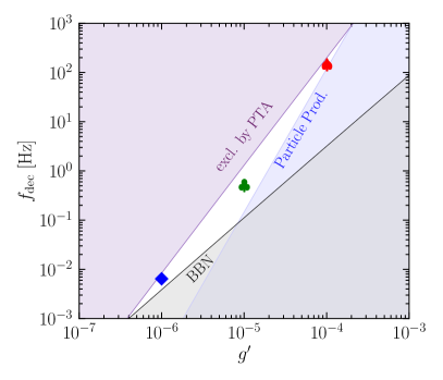
In this Letter, we show that the -dependent GW spectrum and a concrete link between GWs and high-scale leptogenesis can be achieved in the context of model with a peculiar scalar field dynamics [25]. After the phase transition, rolls down to its true vacuum and oscillates coherently to provide an early matter-domination when it is long-lived. If the lifetime of the scalar field gets determined by and , then regulates the beginning and the end of the matter-domination. Differently from Ref. [12], the amplitude and the spectral features of the GWs radiated from cosmic strings are imprinted by the -dependent matter domination, thus carrying information on , and therefore, different regimes of flavored leptogenesis. In particular, the scale invariance in the GW spectrum at higher frequencies breaks at a frequency determined by the end of the matter domination at the temperature (see Fig. 1). We point out that such a scenario allows us to probe the RHN mass scale markedly, in agreement with all the relevant constraints on the parameter space (see Fig. 2): i) the bound from the recent observations of nHz GWs by Pulsar Timing Arrays (PTA) [26, 27, 28, 29, 30] which disfavor GWs from cosmic strings [31]; ii) the condition that the cosmic strings radiate predominantly GWs than particles [32, 33]; iii) the requirement that the decays before the Big-Bang-Nucleosynthesis (BBN) [34, 35]. We highlight that if the break of the GW spectrum occurs in the LISA (ET) frequency band, most likely it is a signature of a 3FL (2FL) regime. Remarkably, the amplitudes and the spectral break frequencies of the GW spectra predicted by our model are very well delimited and they are all within reach of planned gravitational wave experiments such as LISA, DECIGO and ET [36, 37, 38]. This ensures unique and highly testable GW signatures of flavor regimes of high-scale leptogenesis.
The parameter space for -dependent matter domination. The seesaw Lagrangian for neutrino masses and leptogenesis is given by
| (1) |
where is the neutrino Dirac Yukawa coupling and is the SM Higgs (lepton doublet). The fields and have charge , whereas the same charges for and are and , respectively. The scalar field dynamics is dictated by the finite temperature potential restoring symmetry at higher temperatures given by [39, 40]
| (2) |
where and are functions of gauge coupling , is the self-interaction coupling, and the zero temperature potential determines the vacuum expectation value . The last term in Eq. (2) generates a potential barrier causing a secondary minimum at , which becomes degenerate with the one at . The potential barrier vanishes at , and the minimum at becomes a maximum. The transition from to can be treated as a second-order transition with an extremely quick disappearance of the potential barrier if the order parameter (weakly first-order transition). Such a smooth transition can be obtained approximately within the ballpark of and for [13, 41]. Once rolls down, it oscillates around behaving as matter [42, 43, 25]. Three important observations are in order. First, the breaking scale can be as high as the GUT scale, implying . Second, the Hubble friction at should also be negligible for the rolling of the field down to ; this can be achieved by considering larger than the Hubble parameter . Third, RHNs become massive after the phase transition at . Therefore, the scale of leptogenesis is bounded from above as .
We aim to make long-lived to induce a matter-domination epoch with a lifetime determined by and . In high-scale leptogenesis scenario, the coupling should be generically large to have comparable with . In such a case, if , tree-level decay of to RHN pairs () would be too quick to make long-lived. This restricts ourselves to the case . Therefore, along with , the scalar is long-lived within the folowing range
| (3) |
where we have assumed . In this case, the mass of is suppressed by a factor compared to the , thus kinematically forbidding the tree-level decays of to pairs. Note interestingly that the seesaw Lagrangian in Eq. (1) can provide an effective coupling at one-loop to trigger decay. Therefore, despite being large, we can have a smaller decay rate as it is proportional to . This decay involves both: the RHN mass and the active neutrino mass via the Dirac Yukawa coupling . In our discussion, we shall consider this radiative decay with the assumption that . The decay rate up to a logarithmic factor is given by [44, 45, 25]
| (4) |
with . We have assumed eV, the SM Higgs vacuum expectation value GeV, and , which implies . The latter assumption should not drastically change the phenomenological implication of the scenario because of the constraint in Eq. (3).
The evolution of the energy density of and the duration of matter domination epoch, which ends when decay [25], can be tracked by solving the Friedman equations (see Supplemental Material I for further details). The decay temperature of the scalar field can be obtained analytically considering , and is given by
| (5) |
where we consider . The scalar decays must occur before BBN, i.e., . Moreover, because the scalar field is long-lived, it produces entropy which dilutes any pre-existing relic, including the baryon asymmetry. The amount of entropy production in our scenario can be computed as . The entropy dilution by a factor of must be considered in the computation of baryon asymmetry. Even in the low region, the scenario does not allow large entropy dilution [25], consequently the baryon asymmetry can be comfortably generated. Finally, we mention that we can safely neglect the additional one-loop decay (the two-body decay is suppressed due to chirality flip [46]), where and are SM fermions and vector bosons. Indeed, this decay dominates over the only for and smaller values of , which is outside our parameter space.
Imprints of flavored leptogenesis on GWs from cosmic string. Gravitational waves are radiated from cosmic string loops chopped off from the long strings resulting from the spontaneous breaking of the gauged [23, 24]. Long strings are described by a correlation length , with is the long string energy density and is the string tension defined as [47]
| (6) |
for . In the present analysis, we take therefore . The time evolution of a radiating loop of initial size is given by , where [23, 24], [48, 49], , and being the initial time of loop creation. The total energy loss from a loop is decomposed into a set of normal-mode oscillations with frequencies , where , is the present-day frequency at , and is the scale factor. The total GW energy density is computed by summing all the modes giving [48, 49]
| (7) |
where is the critical energy density of the universe, is an efficiency factor [48] and is the loop number density. The latter can be computed from the velocity-dependent-one-scale model as [50, 51, 52, 53]
| (8) |
where with being the equation of state parameter of the universe, and () for radiation-dominated (matter-dominated) universe [53]. The quantity quantifies the emitted power in -th mode, with () for loops containing cusps (kinks) [54]. We shall present the results for the dominant mode which captures the qualitative features of our analysis.
The integral in Eq. (7) is subjected to two Heaviside functions which set cut-offs on the GW spectrum at very high frequencies above which it falls as . The quantity represents the time until which the motion of the string network is damped by friction [55], and is a critical length above which GW emission is dominant over particle production as shown by high-resolution numerical simulations [32, 33]. The critical length is where is the width of the string and () for loops containing cusps (kinks). Note that we deal with small values of leading to “fat” strings, which are not conventional while studying GWs signatures from cosmic strings in BSM models [12]. In particular, in this case, the particle production cut-off in the GW spectrum is much stronger than the one usually considered for “thin strings” (). Thus, our scenario is also the first concrete BSM model that discusses the results of [32, 33] for small .
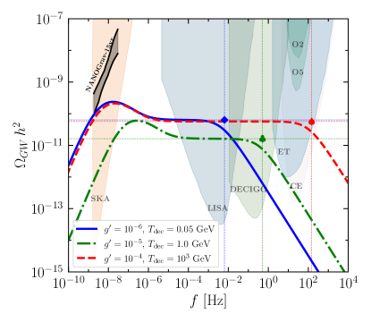
In Fig. 1, we show the GW spectrum from Eq. (7) (for ) predicted by our model for three benchmark scenarios: and (blue line), and (green line), and (red line), with the scale of leptogenesis being uniquely defined by Eq. (5) to be , and in units of GeV, respectively. Without any intermediate matter-dominated epoch, the GW spectrum has two main contributions: a low-frequency peak owing to the GW radiation from the loops which are created in the radiation epoch and decay in the standard matter epoch, and an almost scale-invariant plateau at high frequencies as [48, 49, 56]
| (9) |
that arises from loop creation and decay in the radiation-dominated epoch only. In Eq. (9), , and . Note that , implying, the larger the symmetry breaking scale, the stronger the amplitude of GW. In our scenario, which features instead an intermediate matter-dominated epoch, the plateau breaks at a high frequency , beyond which the spectrum falls as (see Fig. 1). The analytical expression for this spectral break frequency can be computed as [57]
| (10) |
where is the red-shift at the standard matter-radiation equality taking place at time , while is the time at which the scalar field decays (matter domination ends). For the three benchmark cases in Fig. 1, the break of the GW spectrum occurs in the LISA [36], DECIGO [37] and ET [38] frequency bands, respectively.
In order to robustly claim the spectral fall as a signature of -dependent matter domination, we must require both and . The first condition leads to the constraint
| (11) |
with GeV. Similar constraints can be derived for loops containing kinks, which however are less stringent. The second condition implies
| (12) |
with GeV.
The parameter space of our model is also constrained by the recent PTA observations of stochastic GW which disfavor cosmic strings due to a different spectral slope [31]. Thus, PTA data require at nHz giving . This translates to the constraint on as
| (13) |
whit GeV. All these constrained are satisfied by the benchmark cases shown in Fig. 1.
We note that there could be additional contribution to the GW spectrum at very high frequencies due to the cosmic string loops in the first radiation epoch before starts to dominate. However, the amplitude at higher frequencies is suppressed not only because of the entropy production, but also because the hard particle production cut-off makes the spectrum red.
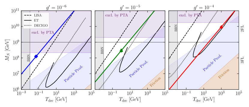
Results and discussion. In Fig. 2, we show the sensitivities of LISA, DECIGO and ET in the plane -, assuming (left panel), (middle panel) and (right panel), together with all the conditions and constraints discussed above. We underline that the dependence of the GW sensitivities on comes from the relation . The white regions in each plot can be generally regarded as allowed parameter space when taking and as independent parameters. However, in our model, they are related by Eq. (5) which restricts the allowed parameter space along the solid colored lines in the plots. Overall, the requirement of negligible particle production from cosmic string, the recent PTA data, and the BBN constraint limit the parameter space to be and .
We find that, irrespective of the values of , going from light to heavy region along the colored lines, the spectral break frequency increases according to Eq.s (5) and (10). This trend allows us to point out that if the spectral break occurs in the LISA band, it most likely corresponds to (3FL regime), as proven by the allowed segment of the blue line in the left plot. With a similar argument, a spectral break in the ET band would correspond to a 2FL regime of leptogenesis, as depicted by the red line in the right plot. An intermediate situation with , both the 2FL and 3FL regions would provide a spectral break in the DECIGO frequency band. Therefore, in this frequency band, the spectral break signature of 2FL and 3FL becomes ambiguous.
The allowed parameter space of our model can be translated into allowed regions for the GW plateau amplitude and the break frequency (see Supplemental Material II for details). Usually, they are limited from above by the PTA data. However, in our model, they are also bounded from below by the BBN constraint due to the matter-dominated epoch and by the requirement that the spectral break is not due to the particle production from cosmic strings. We find that our scenario implies and which we define as the Gravitational Waves windows for Flavored Regimes of Leptogenesis (GWFRL). These ranges, within which a robust GW signature of high-scale leptogenesis is achieved, will be fully explored by planned GW experiments such as LISA, DECIGO and ET. These GWFRL windows also trivially satisfy two important constraints. First, due to the Hubble friction being always less than at . Second, the ratio of the vacuum energy to the radiation at , which in our case is , is always smaller than one, thus avoiding a second period of inflation.
There could be possible corrections to the GWFRL windows relaxing some of our assumptions. First, we have considered but a more rigorous parameter space scan could be performed to find a smooth transition of the field and at the same time being consistent with other gauge coupling dependent constraints and a negligible decays. Second, we have presented our results on GWs for mode. However, when summing over a large number of modes, the overall amplitude and the spectral break frequency would change slightly. Third, we have assumed . Weakening this assumption but being still consistent with Eq. (3) would anyway not modify the overall trend of the parameter space. Indeed, smaller () would correspond to smaller and therefore smaller , meaning a 3FL regime likely to show up the spectral break at lower frequencies than the 2FL regime. Summarizing, we point out that the GWFRL windows we have derived in the present paper are quite robust against our assumptions. In conclusions, we demonstrate that different flavor regimes of high-scale leptogenesis can be realistically probed with GW signatures from cosmic strings, thus establishing synergy between low-energy neutrino physics and gravitational waves.
Acknowledgements: We thank Tanmay Vachaspati for useful insight regarding the particle production cut-off. The work of MC, GM, RS, and NS is supported by the research project TAsP (Theoretical Astroparticle Physics) funded by the Istituto Nazionale di Fisica Nucleare (INFN). The work of NS is further supported by the research grant number 2022E2J4RK “PANTHEON: Perspectives in Astroparticle and Neutrino THEory with Old and New messengers” under the program PRIN 2022 funded by the Italian Ministero dell’Università e della Ricerca (MUR). The work of SD is supported by the National Natural Science Foundation of China (NNSFC) under grant No. 12150610460.
References
- Fukugita and Yanagida [1986] M. Fukugita and T. Yanagida, Phys. Lett. B 174, 45 (1986).
- Ade et al. [2016] P. A. R. Ade et al. (Planck), Astron. Astrophys. 594, A13 (2016), arXiv:1502.01589 [astro-ph.CO] .
- Kuzmin et al. [1985] V. A. Kuzmin, V. A. Rubakov, and M. E. Shaposhnikov, Phys. Lett. B 155, 36 (1985).
- Davidson et al. [2008] S. Davidson, E. Nardi, and Y. Nir, Phys. Rept. 466, 105 (2008), arXiv:0802.2962 [hep-ph] .
- Buchmuller et al. [2005] W. Buchmuller, P. Di Bari, and M. Plumacher, Annals Phys. 315, 305 (2005), arXiv:hep-ph/0401240 .
- Abada et al. [2006] A. Abada, S. Davidson, A. Ibarra, F. X. Josse-Michaux, M. Losada, and A. Riotto, JHEP 09, 010 (2006), arXiv:hep-ph/0605281 .
- Nardi et al. [2006] E. Nardi, Y. Nir, E. Roulet, and J. Racker, JHEP 01, 164 (2006), arXiv:hep-ph/0601084 .
- Blanchet and Di Bari [2007] S. Blanchet and P. Di Bari, JCAP 03, 018 (2007), arXiv:hep-ph/0607330 .
- Pascoli et al. [2007] S. Pascoli, S. T. Petcov, and A. Riotto, Nucl. Phys. B 774, 1 (2007), arXiv:hep-ph/0611338 .
- Abe et al. [2018] K. Abe et al. (T2K), Phys. Rev. Lett. 121, 171802 (2018), arXiv:1807.07891 [hep-ex] .
- Acero et al. [2018] M. A. Acero et al. (NOvA), Phys. Rev. D 98, 032012 (2018), arXiv:1806.00096 [hep-ex] .
- Dror et al. [2020] J. A. Dror, T. Hiramatsu, K. Kohri, H. Murayama, and G. White, Phys. Rev. Lett. 124, 041804 (2020), arXiv:1908.03227 [hep-ph] .
- Blasi et al. [2020] S. Blasi, V. Brdar, and K. Schmitz, Phys. Rev. Res. 2, 043321 (2020), arXiv:2004.02889 [hep-ph] .
- Samanta and Datta [2021] R. Samanta and S. Datta, JHEP 05, 211 (2021), arXiv:2009.13452 [hep-ph] .
- Datta et al. [2021] S. Datta, A. Ghosal, and R. Samanta, JCAP 08, 021 (2021), arXiv:2012.14981 [hep-ph] .
- Davidson [1979] A. Davidson, Phys. Rev. D 20, 776 (1979).
- Marshak and Mohapatra [1980] R. E. Marshak and R. N. Mohapatra, Phys. Lett. B 91, 222 (1980).
- Buchmüller et al. [2013] W. Buchmüller, V. Domcke, K. Kamada, and K. Schmitz, JCAP 10, 003 (2013), arXiv:1305.3392 [hep-ph] .
- Buchmuller et al. [2020] W. Buchmuller, V. Domcke, H. Murayama, and K. Schmitz, Phys. Lett. B 809, 135764 (2020), arXiv:1912.03695 [hep-ph] .
- Kibble [1976] T. W. B. Kibble, J. Phys. A 9, 1387 (1976).
- Hindmarsh and Kibble [1995] M. B. Hindmarsh and T. W. B. Kibble, Rept. Prog. Phys. 58, 477 (1995), arXiv:hep-ph/9411342 .
- Jeannerot et al. [2003] R. Jeannerot, J. Rocher, and M. Sakellariadou, Phys. Rev. D 68, 103514 (2003), arXiv:hep-ph/0308134 .
- Vilenkin [1981] A. Vilenkin, Phys. Lett. B 107, 47 (1981).
- Vachaspati and Vilenkin [1985] T. Vachaspati and A. Vilenkin, Phys. Rev. D 31, 3052 (1985).
- Chianese et al. [2024] M. Chianese, S. Datta, R. Samanta, and N. Saviano, (2024), arXiv:2405.00641 [hep-ph] .
- Agazie et al. [2023] G. Agazie et al. (NANOGrav), Astrophys. J. Lett. 951, L8 (2023), arXiv:2306.16213 [astro-ph.HE] .
- Antoniadis et al. [2023a] J. Antoniadis et al. (EPTA, InPTA:), Astron. Astrophys. 678, A50 (2023a), arXiv:2306.16214 [astro-ph.HE] .
- Reardon et al. [2023] D. J. Reardon et al., Astrophys. J. Lett. 951, L6 (2023), arXiv:2306.16215 [astro-ph.HE] .
- Xu et al. [2023] H. Xu et al., Res. Astron. Astrophys. 23, 075024 (2023), arXiv:2306.16216 [astro-ph.HE] .
- Antoniadis et al. [2023b] J. Antoniadis et al. (EPTA), (2023b), arXiv:2306.16227 [astro-ph.CO] .
- Afzal et al. [2023] A. Afzal et al. (NANOGrav), Astrophys. J. Lett. 951, L11 (2023), arXiv:2306.16219 [astro-ph.HE] .
- Matsunami et al. [2019] D. Matsunami, L. Pogosian, A. Saurabh, and T. Vachaspati, Phys. Rev. Lett. 122, 201301 (2019), arXiv:1903.05102 [hep-ph] .
- Auclair et al. [2020a] P. Auclair, D. A. Steer, and T. Vachaspati, Phys. Rev. D 101, 083511 (2020a), arXiv:1911.12066 [hep-ph] .
- Cyburt et al. [2016] R. H. Cyburt, B. D. Fields, K. A. Olive, and T.-H. Yeh, Rev. Mod. Phys. 88, 015004 (2016), arXiv:1505.01076 [astro-ph.CO] .
- Hasegawa et al. [2019] T. Hasegawa, N. Hiroshima, K. Kohri, R. S. L. Hansen, T. Tram, and S. Hannestad, JCAP 12, 012 (2019), arXiv:1908.10189 [hep-ph] .
- Amaro-Seoane et al. [2017] P. Amaro-Seoane et al. (LISA), (2017), arXiv:1702.00786 [astro-ph.IM] .
- Kawamura et al. [2006] S. Kawamura et al., Class. Quant. Grav. 23, S125 (2006).
- Sathyaprakash et al. [2012] B. Sathyaprakash et al., Class. Quant. Grav. 29, 124013 (2012), [Erratum: Class.Quant.Grav. 30, 079501 (2013)], arXiv:1206.0331 [gr-qc] .
- Linde [1979] A. D. Linde, Rept. Prog. Phys. 42, 389 (1979).
- Kibble [1980] T. W. B. Kibble, Phys. Rept. 67, 183 (1980).
- Datta and Samanta [2023] S. Datta and R. Samanta, Phys. Rev. D 108, L091706 (2023), arXiv:2307.00646 [hep-ph] .
- Masso et al. [2005] E. Masso, F. Rota, and G. Zsembinszki, Phys. Rev. D 72, 084007 (2005), arXiv:astro-ph/0501381 .
- Datta and Samanta [2022] S. Datta and R. Samanta, JHEP 11, 159 (2022), arXiv:2208.09949 [hep-ph] .
- Gross et al. [2016] C. Gross, O. Lebedev, and M. Zatta, Phys. Lett. B 753, 178 (2016), arXiv:1506.05106 [hep-ph] .
- Enqvist et al. [2016] K. Enqvist, M. Karciauskas, O. Lebedev, S. Rusak, and M. Zatta, JCAP 11, 025 (2016), arXiv:1608.08848 [hep-ph] .
- Han and Wang [2017] T. Han and X. Wang, JHEP 10, 036 (2017), arXiv:1704.00790 [hep-ph] .
- Hill et al. [1988] C. T. Hill, H. M. Hodges, and M. S. Turner, Phys. Rev. D 37, 263 (1988).
- Blanco-Pillado et al. [2014] J. J. Blanco-Pillado, K. D. Olum, and B. Shlaer, Phys. Rev. D 89, 023512 (2014), arXiv:1309.6637 [astro-ph.CO] .
- Blanco-Pillado and Olum [2017] J. J. Blanco-Pillado and K. D. Olum, Phys. Rev. D 96, 104046 (2017), arXiv:1709.02693 [astro-ph.CO] .
- Martins and Shellard [1996] C. J. A. P. Martins and E. P. S. Shellard, Phys. Rev. D 54, 2535 (1996), arXiv:hep-ph/9602271 .
- Martins and Shellard [2002] C. J. A. P. Martins and E. P. S. Shellard, Phys. Rev. D 65, 043514 (2002), arXiv:hep-ph/0003298 .
- Sousa and Avelino [2013] L. Sousa and P. P. Avelino, Phys. Rev. D 88, 023516 (2013), arXiv:1304.2445 [astro-ph.CO] .
- Auclair et al. [2020b] P. Auclair et al., JCAP 04, 034 (2020b), arXiv:1909.00819 [astro-ph.CO] .
- Damour and Vilenkin [2001] T. Damour and A. Vilenkin, Phys. Rev. D 64, 064008 (2001), arXiv:gr-qc/0104026 .
- Vilenkin [1991] A. Vilenkin, Phys. Rev. D 43, 1060 (1991).
- Sousa et al. [2020] L. Sousa, P. P. Avelino, and G. S. F. Guedes, Phys. Rev. D 101, 103508 (2020), arXiv:2002.01079 [astro-ph.CO] .
- Cui et al. [2019] Y. Cui, M. Lewicki, D. E. Morrissey, and J. D. Wells, JHEP 01, 081 (2019), arXiv:1808.08968 [hep-ph] .
Supplemental Material for
Probing flavored regimes of leptogenesis with gravitational waves from cosmic strings
Marco Chianese, Satyabrata Datta, Gennaro Miele, Rome Samanta, and Ninetta Saviano
The Supplemental Material is organized as follows. In Sec. I, we discuss the evolution of the radiation and the scalar field energy densities, and the produced entropy with the inverse of temperature. We derive the analytical expressions for the decay temperature and the amount of the produced entropy which match the numerical results well. In Sec. II, we detail the constraints leading to the Gravitational Waves window for Flavored Regimes of Leptogenesis (GWFRL).
I scalar field evolution and entropy production
The scalar field with initial vacuum energy dominates the energy density for a period, and injects entropy as it decays. We account for this effect by solving the following Friedmann equations:
| (S1) |
and upon recasting them as
| (S2) |
where and are the energy densities of radiona and the scalar field as a function of, is the Hubble parameter, is the entropy density of the thermal bath, and the temperature-time relation has been derived from the third of Eq. (S1) as
| (S3) |
with and being the scale factor and the number of degree of freedom, respectively. The production of entropy from the decays is computed by solving
| (S4) |
and computing the ratio of after and before the scalar field decay. The amount of entropy production can be analytically quantified as
| (S5) |
by considering which gives the decay temperature
| (S6) |
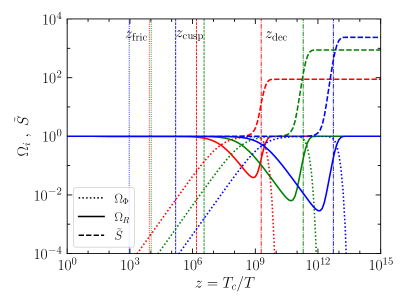
with being the reduced Planck constant, and is the effective degrees of freedom that contribute to the radiation. The evolution of the radiation, the scalar field normalized energy densities , and the entropy production factor corresponding to the benchmarks discussed in the main text are shown in Fig. S1.
II Gravitational Waves window for Flavored Regimes of Leptogenesis (GWFRL)
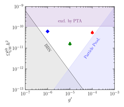
We here detail the upper and lower bounds on the the GW plateau amplitude and the break frequency which allow us to define the GWFRL windows reported in Fig. S2. These regions are bounded from below by either the BBN or the particle production constraint, and from above by the PTA observations. The lower bounds on the GW amplitude (from Eq. (9)) come from the lower bound on imposed by BBN and particle production from cosmic strings, which read
| (S7) | |||||
| (S8) |
Similarly, the lower bounds on the spectral break frequency are derived as
| (S9) | |||||
| (S10) |
The upper bound on the plateau amplitude is given by
| (S11) |
while for we have
| (S12) |