Graph Neural Preconditioners for Iterative Solutions of Sparse Linear Systems

Abstract

Preconditioning is at the heart of iterative solutions of large, sparse linear systems of equations in scientific disciplines. Several algebraic approaches, which access no information beyond the matrix itself, are widely studied and used, but ill-conditioned matrices remain very challenging. We take a machine learning approach and propose using graph neural networks as a general-purpose preconditioner. They show attractive performance for ill-conditioned problems, in part because they better approximate the matrix inverse from appropriately generated training data. Empirical evaluation on over 800 matrices suggests that the construction time of these graph neural preconditioners (GNPs) is more predictable than other widely used ones, such as ILU and AMG, while the execution time is faster than using a Krylov method as the preconditioner, such as in inner-outer GMRES. GNPs have a strong potential for solving large-scale, challenging algebraic problems arising from not only partial differential equations, but also economics, statistics, graph, and optimization, to name a few.

1 Introduction

Iterative methods are commonly used to solve large, sparse linear systems of equations $\mathbf{A}\mathbf{x}=\mathbf{b}$. These methods typically build a Krylov subspace, onto which the original system is projected, such that an approximate solution within the subspace is extracted. For example, GMRES [30], one of the most popularly used methods in practice, builds an orthonormal basis $\{\mathbf{v}_{1},\mathbf{v}_{2},\ldots,\mathbf{v}_{m}\}$ of the $m$-dimensional Krylov subspace by using the Arnoldi process and defines the approximate solution $\mathbf{x}_{m}\in\mathbf{x}_{0}+\operatorname{span}(\{\mathbf{v}_{1},\mathbf{v}_{2},\ldots,\mathbf{v}_{m}\})$, such that the residual norm $\|\mathbf{b}-\mathbf{A}\mathbf{x}_{m}\|_{2}$ is minimized.

The effectiveness of Krylov methods heavily depends on the conditioning of the matrix $\mathbf{A}$. Hence, designing a good preconditioner is critical in practice. In some cases (e.g., solving partial differential equations, PDEs), the problem structure provides additional information that aids the development of a preconditioner applicable to this problem or a class of similar problems. For example, multigrid preconditioners are particularly effective for Poisson-like problems with a mesh. In other cases, little information is known beyond the matrix itself. An example is the SuiteSparse matrix collection [8], which contains thousands of sparse matrices for benchmarking numerical linear algebra algorithms. In these cases, a general-purpose (also called “algebraic”) preconditioner is desirable; examples include ILU [28], approximate inverse [7], and algebraic multigrid (AMG) [27]. However, it remains very challenging to design one that performs well universally.

In this work, we propose to use neural networks as a general-purpose preconditioner. Specifically, we consider preconditioned Krylov methods for solving problems in the form $\mathbf{A}\mathbf{M}\mathbf{u}=\mathbf{b}$, where $\mathbf{M}\approx\mathbf{A}^{-1}$ is the preconditioner, $\mathbf{u}$ is the new unknown, and $\mathbf{x}=\mathbf{M}\mathbf{u}$ is the recovered solution. We design a graph neural network (GNN) [35, 33] to assume the role of $\mathbf{M}$ and develop a training method to learn $\mathbf{M}$ from select $(\mathbf{b},\mathbf{x})$ pairs. This proposal is inspired by the universal approximation property of neural networks [12] and encouraged by their widespread success in artificial intelligence [2]. We use a GNN to approximate the mapping from the right-hand side $\mathbf{b}$ to the solution $\mathbf{x}$.

Because a neural network is, in nature, nonlinear, our preconditioner $\mathbf{M}$ is not a linear operator anymore. We can no longer build a Krylov subspace for $\mathbf{A}\mathbf{M}$ when a Krylov subspace is defined for only linear operators. Hence, we focus on flexible variants of the preconditioned Krylov methods instead. Specifically, we use flexible GMRES (FGMRES) [29], which considers $\mathbf{M}$ to be different in every Arnoldi step. In this framework, all what matters is the subspace from which the approximate solution is extracted. A nonlinear operator $\mathbf{M}$ can also be used to build this subspace and hence the neural preconditioner is applicable to FGMRES.

There are a few advantages of the proposed graph neural preconditioner (GNP). It performs comparatively much better for ill-conditioned problems, by learning the matrix inverse from data, mitigating the restrictive modeling of the sparsity pattern (as in ILU and approximate inverse), the insufficient quality of polynomial approximation (as in using Krylov methods as the preconditioner), and the challenge of smoothing over a non-geometric mesh (as in AMG). Additionally, empirical evaluation suggests that the construction time of GNP is more predictable, inherited from the predictability of neural network training, than that of ILU and AMG; and the execution time of GNP is much shorter than GMRES as the preconditioner, which may be bottlenecked by the orthogonalization in the Arnoldi process.

1.1 Contributions

Our work has a few technical contributions. First, we offer a convergence analysis for FGMRES. Although this method is well known and used in practice, little theoretical work was done, in part because the tools for analyzing Krylov subspaces are not readily applicable (as the subspace is no longer Krylov and we have no isomorphism with the space of polynomials). Instead, our analysis is a posteriori, based on the computed subspace.

Second, we propose an effective approach to training the neural preconditioner; in particular, training data generation. While it is straightforward to train the neural network in an online-learning manner—through preparing streaming, random input-output pairs in the form of $(\mathbf{b},\mathbf{x})$—it leaves open the question regarding what randomness best suits the purpose. We consider the bottom eigen-subspace of $\mathbf{A}$ when defining the sampling distribution.

Third, we develop a scale-equivariant GNN as the preconditioner. Because of the way that training data are generated, the GNN inputs $\mathbf{b}$ can have vast different scales; meanwhile, the ground truth operator $\mathbf{A}^{-1}$ is equivariant to the scaling of the inputs. Hence, to facilitate training, we design the GNN by imposing an inductive bias that obeys scale-equivariance.

Fourth, we adopt a novel evaluation protocol for general-purpose preconditioners. The common practice evaluates a preconditioner on a limited number of problems; in many occasions, these problems come from a certain type of PDEs or an application, which constitutes only a portion of the use cases of solving linear systems. To broadly evaluate a new kind of general-purpose preconditioner and understand its strengths and weaknesses, we propose to test it on a large number of matrices commonly used by the community. To this end, we use the SuiteSparse collection and perform evaluation on a substantial portion of it (all non-SPD, real matrices falling inside a size interval; over 800 in this work). To streamline the evaluation, we define evaluation criteria, limit the tuning of hyperparameters, and study statistics over the distribution of matrices.

1.2 Related Work

It is important to put the proposed GNP in context. The idea of using a neural network to construct a preconditioner emerged recently. The relevant approaches learn the nonzero entries of the incomplete LU/Cholesky factors [20, 11] or of the approximate inverse [3]. In these approaches, the neural network as a function does not directly approximate the mapping from $\mathbf{b}$ to $\mathbf{x}$ like ours does; rather, it is used to complete the nonzeros of the predefined sparsity structure.

Approaches wherein the neural network directly approximates the matrix inverse are more akin to physics-informed neural networks (PINNs) [26] and neural operators (NOs) [17, 21, 22, 23]. However, the learning of PINNs requires a PDE (i.e., the physics) whose residual forms a training loss, whereas NOs consider infinite-dimensional function spaces, with PDEs being the primary application. In our case of a general-purpose preconditioner, there is not an underlying PDE; and not every matrix problem relates to function spaces with additional properties to exploit (e.g., spatial coordinates, smoothness, and decay of the Green’s function). For example, one may be interested in finding the commute times between a node and all other nodes in a graph; this problem can be solved by solving a linear system with respect the graph Laplacian matrix. The only information we exploit is the matrix itself.

2 Method

Let $\mathbf{A}\in\mathbb{R}^{n\times n}$. From now on, $\mathbf{M}$ is an operator $\mathbb{R}^{n}\to\mathbb{R}^{n}$ and we write $\mathbf{M}(\mathbf{v})$ to mean applying the operator on $\mathbf{v}\in\mathbb{R}^{n}$. This notation includes the special case $\mathbf{M}(\mathbf{v})=\mathbf{M}\mathbf{v}$ when $\mathbf{M}$ is a matrix.

2.1 Flexible GMRES

A standard preconditioned Krylov solver solves the linear system $\mathbf{A}\mathbf{M}\mathbf{u}=\mathbf{b}$ by viewing $\mathbf{A}\mathbf{M}$ as the new matrix and building a Krylov subspace, from which an approximate solution $\mathbf{u}_{m}$ is extracted and $\mathbf{x}_{m}$ is recovered from $\mathbf{M}\mathbf{u}_{m}$. It is important to note that a subspace, by definition, is linear. However, applying a nonlinear operator $\mathbf{M}$ on the linear vector space does not result in a vector space spanned by the mapped basis. Hence, convergence theory of $\mathbf{x}_{m}=\mathbf{M}(\mathbf{u}_{m})$ is broken.

We resort to flexible variants of Krylov solvers [29, 25, 6] and focus on flexible GMRES for simplicity. FGMRES was designed such that the matrix $\mathbf{M}$ can change in each Arnoldi step; we extend it to a fixed, but nonlinear, operator.

Algorithm 1 FGMRES with $\mathbf{M}$ being a nonlinear operator

1:Let $\mathbf{x}_{0}$ be given. Define $\overline{\mathbf{H}}_{m}\in\mathbb{R}^{(m+1)\times m}$ and initialize all its entries $h_{ij}$ to zero

2:loop until maxiters is reached

3:     Compute $\mathbf{r}_{0}=\mathbf{b}-\mathbf{A}\mathbf{x}_{0}$, $\beta=\|\mathbf{r}_{0}\|_{2}$, and $\mathbf{v}_{1}=\mathbf{r}_{0}/\beta$

4:     for $j=1,\ldots,m$ do

5:         Compute $\mathbf{z}_{j}=\mathbf{M}(\mathbf{v}_{j})$ and $\mathbf{w}=\mathbf{A}\mathbf{z}_{j}$

6:         for $i=1,\ldots,j$ do

7:              Compute $h_{ij}=\mathbf{w}^{\top}\mathbf{v}_{i}$ and $\mathbf{w}\leftarrow\mathbf{w}-h_{ij}\mathbf{v}_{i}$

8:         end for

9:         Compute $h_{j+1,j}=\|\mathbf{w}\|_{2}$ and $\mathbf{v}_{j+1}=\mathbf{w}/h_{j+1,j}$

10:     end for

11:     Define $\mathbf{Z}_{m}=[\mathbf{z}_{1},\ldots,\mathbf{z}_{m}]$ and compute $\mathbf{x}_{m}=\mathbf{x}_{0}+\mathbf{Z}_{m}\mathbf{y}_{m}$ where $\mathbf{y}_{m}=\operatorname*{argmin}_{\mathbf{y}}\|\beta\mathbf{e}_{1}-\overline{\mathbf{H}}_{m}\mathbf{y}\|_{2}$

12:     If $\|\mathbf{b}-\mathbf{A}\mathbf{x}_{m}\|_{2}<\texttt{tol}$, exit the loop; otherwise, set $\mathbf{x}_{0}\leftarrow\mathbf{x}_{m}$

13:end loop

Algorithm 1 summarizes the solver. The algorithm assumes a restart length $m$. Starting from an initial guess $\mathbf{x}_{0}$ with residual vector $\mathbf{r}_{0}$ and 2-norm $\beta$, FGMRES runs $m$ Arnoldi steps, resulting in the relation

$$\mathbf{A}\mathbf{Z}_{m}=\mathbf{V}_{m}\mathbf{H}_{m}+h_{m+1,m}\mathbf{v}_{m+1}\mathbf{e}_{m}^{\top}=\mathbf{V}_{m+1}\overline{\mathbf{H}}_{m},$$ (1)

where $\mathbf{V}_{m}=[\mathbf{v}_{1},\ldots,\mathbf{v}_{m}]\in\mathbb{R}^{n\times m}$ is orthonormal, $\mathbf{Z}_{m}=[\mathbf{z}_{1},\ldots,\mathbf{z}_{m}]\in\mathbb{R}^{n\times n}$ contains $m$ columns $\mathbf{z}_{j}=\mathbf{M}(\mathbf{v}_{j})$, $\mathbf{H}_{m}=[h_{ij}]\in\mathbb{R}^{m\times m}$ is upper Hessenberg, and $\overline{\mathbf{H}}_{m}=[h_{ij}]\in\mathbb{R}^{(m+1)\times m}$ extends $\mathbf{H}_{m}$ with an additional row at the bottom. The approximate solution $\mathbf{x}_{m}$ is computed in the form $\mathbf{x}_{m}\in\mathbf{x}_{0}+\operatorname{span}(\{\mathbf{z}_{1},\ldots,\mathbf{z}_{m}\})=\{\mathbf{x}_{0}+\mathbf{Z}_{m}\mathbf{y}\}$, such that the residual norm $\|\mathbf{b}-\mathbf{A}\mathbf{x}_{m}\|_{2}=\|\beta\mathbf{e}_{1}-\overline{\mathbf{H}}_{m}\mathbf{y}\|_{2}$ is minimized. If the residual norm is sufficiently small, the solution is claimed; otherwise, let $\mathbf{x}_{m}$ be the initial guess of the next Arnoldi cycle and repeat.

We provide a convergence analysis below, which is probably novel.

Theorem 1.

Assume that FGMRES is run without restart and without breakdown. We use the tilde notation to denote the counterpart quantities when FGMRES is run with a fixed preconditioner matrix $\widetilde{\mathbf{M}}$. For any $\widetilde{\mathbf{M}}$ such that $\mathbf{A}\widetilde{\mathbf{M}}$ can be diagonalized, as in $\mathbf{X}^{-1}\mathbf{A}\widetilde{\mathbf{M}}\mathbf{X}=\bm{\Lambda}=\operatorname{diag}(\lambda_{1},\ldots,\lambda_{n})$, the residual $\mathbf{r}_{m}=\mathbf{b}-\mathbf{A}\mathbf{x}_{m}$ satisfies

$$\|\mathbf{r}_{m}\|_{2}\leq\kappa_{2}(\mathbf{X})\epsilon^{(m)}(\bm{\Lambda})\|\mathbf{r}_{0}\|_{2}+\|\mathbf{Q}_{m}\mathbf{Q}_{m}^{\top}-\widetilde{\mathbf{Q}}_{m}\widetilde{\mathbf{Q}}_{m}^{\top}\|_{2}\|\mathbf{r}_{0}\|_{2},$$ (2)

where $\kappa_{2}$ denotes the 2-norm condition number, $\mathbf{Q}_{m}$ (resp. $\widetilde{\mathbf{Q}}_{m}$) is the thin-Q factor of $\mathbf{A}\mathbf{Z}_{m}$ (resp. $\mathbf{A}\widetilde{\mathbf{Z}}_{m}$), $\mathbb{P}_{m}$ denotes the space of degree-$m$ polynomials, and

$$\epsilon^{(m)}(\bm{\Lambda})=\min_{p\in\mathbb{P}_{m},\,p(0)=1}\max_{i=1,\ldots,n}|p(\lambda_{i})|.$$

Let us consider the two terms on the right-hand side of (2). The first term $\kappa_{2}(\mathbf{X})\epsilon^{(m)}(\bm{\Lambda})\|\mathbf{r}_{0}\|_{2}$ is the standard convergence result of GMRES on the matrix $\mathbf{A}\widetilde{\mathbf{M}}$. The factor $\epsilon^{(m)}(\bm{\Lambda})$ is approximately exponential in $m$, when the eigenvalues $\lambda_{i}$ are located in an ellipse which excludes the origin (see [31, Corollary 6.33]). Furthermore, when the eigenvalues are closer to each other than to the origin, the base of the exponential is close to zero, resulting in rapid convergence. Meanwhile, when $\mathbf{A}\widetilde{\mathbf{M}}$ is close to normal, $\kappa_{2}(\mathbf{X})$ is close to 1.

What the nonlinear operator preconditioner $\mathbf{M}$ affects is the second term $\|\mathbf{Q}_{m}\mathbf{Q}_{m}^{\top}-\widetilde{\mathbf{Q}}_{m}\widetilde{\mathbf{Q}}_{m}^{\top}\|_{2}\|\mathbf{r}_{0}\|_{2}$. This term does not show convergence on the surface, but it offers some intuition. Assuming no breakdown, one can always find an $\widetilde{\mathbf{M}}$ such that this term vanishes. Indeed, $\widetilde{\mathbf{M}}=\mathbf{A}^{-1}\mathbf{V}_{n}\mathbf{H}_{n}\mathbf{V}_{n}^{\top}$ makes $\mathbf{A}\mathbf{Z}_{m}=\mathbf{A}\widetilde{\mathbf{Z}}_{m}$, and hence $\mathbf{Q}_{m}=\widetilde{\mathbf{Q}}_{m}$, for all $m$. When the preconditioner $\mathbf{M}$ is close to $\mathbf{A}^{-1}$, $\mathbf{A}\mathbf{Z}_{m}$ is a small perturbation of $\mathbf{V}_{m}$ by definition. Then, (1) suggests that $\overline{\mathbf{H}}_{m}$ is close to the identity matrix for all $m$ and so is $\mathbf{H}_{n}$. Thus, the following corollary characterizes the convergence of the residual.

Corollary 2.

Assume that FGMRES is run without restart and without breakdown. On completion, let $\mathbf{H}_{n}$ be diagonalizable, as in $\mathbf{Y}^{-1}\mathbf{H}_{n}\mathbf{Y}=\bm{\Sigma}=\operatorname{diag}(\sigma_{1},\ldots,\sigma_{n})$. Then, the residual norm satisfies

$$\|\mathbf{r}_{m}\|_{2}\leq\kappa_{2}(\mathbf{Y})\epsilon^{(m)}(\bm{\Sigma})\|\mathbf{r}_{0}\|_{2}\qquad\text{for all $m$}.$$ (3)

2.2 Training Data Generation

We generate a set of $(\mathbf{b},\mathbf{x})$ pairs to train $\mathbf{M}:\mathbf{b}\to\mathbf{x}$. Unlike neural operators where the data generation is costly (e.g., requiring solving PDEs), which limits the training set size, for linear systems, we can sample $\mathbf{x}$ from a certain distribution and obtain $\mathbf{b}=\mathbf{A}\mathbf{x}$ with negligible cost, which creates a streaming training set of $(\mathbf{b},\mathbf{x})$ pairs without size limit.

There is no free lunch. One may sample $\mathbf{x}\sim\mathcal{N}(\mathbf{0},\mathbf{I}_{n})$, which leads to $\mathbf{b}\sim\mathcal{N}(\mathbf{0},\mathbf{A}\mathbf{A}^{\top})$. This distribution is skewed toward the dominant eigen-subspace of $\mathbf{A}\mathbf{A}^{\top}$. Hence, using samples from it for training may result in a poor performance of the preconditioner, when applied to inputs lying close to the bottom eigen-subspace. One may alternatively want the training data $\mathbf{b}\sim\mathcal{N}(\mathbf{0},\mathbf{I}_{n})$, which covers uniformly all possibilities of the preconditioner input on a sphere. However, there are two challenges. First, it requires sampling $\mathbf{x}$ from $\mathcal{N}(\mathbf{0},\mathbf{A}^{-1}\mathbf{A}^{-\top})$, which is a chicken-and-egg problem. Second, $\mathcal{N}(\mathbf{0},\mathbf{A}^{-1}\mathbf{A}^{-\top})$ is also skewed in the spectrum, causing difficulty in network training.

We resort to the Arnoldi process to obtain an approximation of $\mathbf{A}^{-1}\mathbf{A}^{-\top}$, which strikes a balance. Specifically, we run the Arnoldi process in $m$ steps without a preconditioner, which results in a simplification of (1):

$$\mathbf{A}\mathbf{V}_{m}=\mathbf{V}_{m}\mathbf{H}_{m}+h_{m+1,m}\mathbf{v}_{m+1}\mathbf{e}_{m}^{\top}=\mathbf{V}_{m+1}\overline{\mathbf{H}}_{m}.$$ (4)

Let the singular value decomposition of $\overline{\mathbf{H}}_{m}$ be $\mathbf{W}_{m}\mathbf{S}_{m}\mathbf{Z}_{m}^{\top}$, where $\mathbf{W}_{m}\in\mathbb{R}^{(m+1)\times m}$ and $\mathbf{Z}_{m}\in\mathbb{R}^{m\times m}$ are orthonormal and $\mathbf{S}_{m}\in\mathbb{R}^{m\times m}$ is diagonal. We define

$$\mathbf{x}=\mathbf{V}_{m}\mathbf{Z}_{m}\mathbf{S}_{m}^{-1}\bm{\epsilon},\qquad\bm{\epsilon}\sim\mathcal{N}(\mathbf{0},\mathbf{I}_{m}).$$ (5)

Then, with simple algebra we obtain that

$$\mathbf{x} \in\operatorname{range}(\mathbf{V}_{m}), \qquad\mathbf{x} \sim\mathcal{N}(\mathbf{0},\bm{\Sigma}_{m}^{\mathbf{x}}), \qquad\bm{\Sigma}_{m}^{\mathbf{x}} =(\mathbf{V}_{m}\overline{\mathbf{H}}_{m}^{+})(\mathbf{V}_{m}\overline{\mathbf{H}}_{m}^{+})^{\top},$$

$$\mathbf{b} \in\operatorname{range}(\mathbf{V}_{m+1}), \qquad\mathbf{b} \sim\mathcal{N}(\mathbf{0},\bm{\Sigma}_{m}^{\mathbf{b}}), \qquad\bm{\Sigma}_{m}^{\mathbf{b}} =(\mathbf{V}_{m+1}\mathbf{W}_{m})(\mathbf{V}_{m+1}\mathbf{W}_{m})^{\top}.$$

The covariance of $\mathbf{b}$, $\bm{\Sigma}_{m}^{\mathbf{b}}$, is a projector, because both $\mathbf{V}_{m+1}$ and $\mathbf{W}_{m}$ are orthonormal. As $m$ grows, this covariance tends to the identity $\mathbf{I}_{n}$. By the theory of the Arnoldi process [24], $\mathbf{V}_{m+1}$ contains better and better approximations of the extreme eigenvectors as $m$ increases. Hence, $\mathcal{N}(\mathbf{0},\bm{\Sigma}_{m}^{\mathbf{b}})$ has a high density close to the bottom eigen-subspace of $\mathbf{A}$. Of course, because $\bm{\Sigma}_{m}^{\mathbf{b}}$ is low-rank, the distribution has zero density along many directions. Therefore, we sample $\mathbf{x}$ from both $\mathcal{N}(\mathbf{0},\bm{\Sigma}_{m}^{\mathbf{x}})$ and $\mathcal{N}(\mathbf{0},\mathbf{I}_{n})$ to form each training batch, to cover more important subspace directions.

2.3 Scale-Equivariant Graph Neural Preconditioner

We now define the neural network $\mathbf{M}$ that approximates $\mathbf{A}^{-1}$. Naturally, a (sparse) matrix $\mathbf{A}=[a_{ij}]$ admits a graph interpretation, similar to how AMG interpreting the coefficient matrix with a graph. Treating $\mathbf{A}$ as the graph adjacency matrix allows us to use GNNs [16, 10, 32, 34] to parameterize the preconditioner. These neural networks perform graph convolutions in a neighborhood of each node, reducing the quadratic pairwise cost by ignoring nodes faraway from the neighborhood.

Our neural network is based on the graph convolutional network (GCN) [16]. A GCN layer is defined as $\text{GCONV}(\mathbf{X})=\operatorname{ReLU}(\widehat{\mathbf{A}}\mathbf{X}\mathbf{W})$, where $\widehat{\mathbf{A}}\in\mathbb{R}^{n\times n}$ is some normalization of $\mathbf{A}$, $\mathbf{X}\in\mathbb{R}^{n\times d_{\text{in}}}$ is input data, and $\mathbf{W}\in\mathbb{R}^{d_{\text{in}}\times d_{\text{out}}}$ is a learnable parameter.

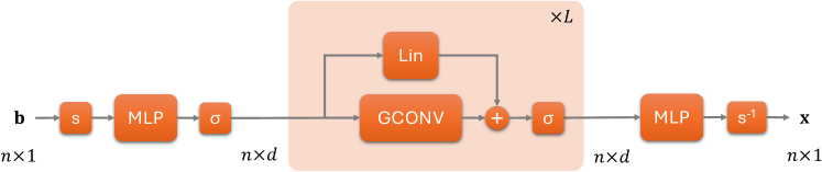
Figure 1: Our GNN architecture for the preconditioner $\mathbf{M}$. The nonlinearity $\sigma$ is $\operatorname{ReLU}$. The component $s$ denotes the scale-equivariant operator (8).

Our neural network, as illustrated in Figure 1, enhances from GCN in a few manners:

1. We normalize $\mathbf{A}$ differently. Specifically, we define

   $$\widehat{\mathbf{A}}=\mathbf{A}/\gamma\quad\text{where}\quad\textstyle\gamma=\min\Big{\{}\max_{i}\big{\{}\sum_{j}|a|_{ij}\big{\}},\max_{j}\big{\{}\sum_{i}|a|_{ij}\big{\}}\Big{\}}.$$ (6)

   The factor $\gamma$ is an upper bound of the spectral radius of $\mathbf{A}$ based on the Gershgorin circle theorem [9]. This avoids division-by-zero that may occur in the standard GCN normalization, because the nonzeros of $\mathbf{A}$ can be both positive and negative.

2. We add a residual connection to GCONV, to allow stacking a deeper GNN. Specifically, we define a Res-GCONV layer to be

   $$\text{Res-GCONV}(\mathbf{X})=\operatorname{ReLU}(\mathbf{X}\mathbf{U}+\widehat{\mathbf{A}}\mathbf{X}\mathbf{W}).$$ (7)

   Moreover, we let the parameters $\mathbf{U}$ and $\mathbf{W}$ be square matrices of dimension $d\times d$, such that the input/output dimensions across layers do not change. We stack $L$ such layers.

3. We use an MLP encoder (resp. MLP decoder) before (resp. after) the $L$ Res-GCONV layers to lift (resp. project) the dimensions.

Additionally, note that the operator to approximate, $\mathbf{A}^{-1}$, is scale-equivariant, but a neural network is not guaranteed so. More importantly, the neural network input $\mathbf{b}$ may have very different scales, due to the sampling approach considered in the preceding subsection. Hence, to facilitate training, we design a parameter-free scaling $s$ and back-scaling $s^{-1}$:

$$\textstyle s(\cdot)=\frac{\sqrt{n}}{\tau}\cdot\quad\text{and}\quad s^{-1}(\cdot)=\frac{\tau}{\sqrt{n}}\,\cdot\,,\quad\text{where }\tau=\|\mathbf{b}\|_{2}.$$ (8)

We apply $s$ at the beginning and $s^{-1}$ at the end of the neural network. Effectively, we restrict the input space of the neural network from the full $\mathbb{R}^{n}$ to a more controllable space—the sphere $\sqrt{n}\mathbb{S}^{n-1}$. Clearly, $s$ guarantees scale-equivariance; i.e., $\mathbf{M}(\alpha\mathbf{b})=\alpha\mathbf{M}(\mathbf{b})$ for any scalar $\alpha\neq 0$.

3 Evaluation Methodology and Experiment Setting

Problems. Our evaluation strives to cover a large number of problems, which come from as diverse application areas as possible. To this end, we turn to the SuiteSparse matrix collection https://sparse.tamu.edu, which is a widely used benchmark in numerical linear algebra. We select all square, real-valued, and non-SPD matrices whose number of rows falls between 1K and 100K and whose number of nonzeros is fewer than 2M. This selection results in 867 matrices with varying densities and applications. Some applications are involved with PDEs (such as computational fluid dynamics), while others come from graph, optimization, economics, and statistics problems.

To facilitate solving the linear systems, we prescale each $\mathbf{A}$ by $\gamma$ defined in (6). This scaling is a form of normalization, which avoids the overall entries of the matrix being exceedingly small or large. All experiments assume the ground truth solution $\mathbf{x}=\mathbf{1}$. FGMRES starts with $\mathbf{x}_{0}=\mathbf{0}$.

Compared methods. We compare GNP with three widely used general-purpose preconditioners: ILU, AMG, and GMRES (using GMRES to precondition GMRES is also called inner-outer GMRES). The endeavor of preconditioning over 800 matrices from different domains limits the choices, but these preconditioners are handy with Python software support. ILU comes from scipy.sparse.linalg.spilu; it in turn comes from SuperLU [18, 19], which implements the thresholded version of ILU [28]. We use the default drop tolerance and fill factor without tuning. AMG comes from PyAMG [1]. Specifically, we use pyamg.blackbox.solver().aspreconditioner as the preconditioner, with the configuration of the blackbox solver computed from pyamg.blackbox.solver_configuration. GMRES is self-implemented. For (the inner) GMRES, we use 10 iterations and stop it when it reaches a relative residual norm tolerance of 1e-6. For (the outer) FGMRES, the restart cycle is 10.

Stopping criteria. The stopping criteria of all linear system solutions are rtol = 1e-8 and maxiters = 100.

Evaluation metrics. Evaluating the solution qualities and comparing different methods for a large number of problems require programmable metrics, but defining these metrics is harder than it appears to be. There are several reasons: (1) not every method reaches rtol within maxiters; (2) the iteration cost for each method is different; and (3) the convergence curves of different methods may cross over. Hence, comparing the number of iterations, the final relative residual norm, or the time, alone, is not enough. We propose two novel metrics. The first one, area under the relative residual norm curve with respect to iterations, is defined as

$$\text{Iter-AUC}=\sum_{i=0}^{\text{iters}}\log_{10}r_{i}-\log_{10}\texttt{rtol},\quad r_{i}=\|\mathbf{b}-\mathbf{A}\mathbf{x}_{i}\|_{2}/\|\mathbf{b}\|_{2},$$

where iters is the actual number of iterations when FGMRES stops and $r_{i}$ is the relative residual norm at iteration $i$. We take logarithm because residual plots are typically done in the log scale. This metric compares methods based on the iteration count, taking into account the history rather than the final error alone.

The second metric, area under the relative residual norm curve with respect to time, is defined as

$$\text{Time-AUC}=\int_{0}^{T}[\log_{10}r(t)-\log_{10}\texttt{rtol}]\,dt\approx\sum_{i=1}^{\text{iters}}[\log_{10}r_{i}-\log_{10}\texttt{rtol}](t_{i}-t_{i-1}),$$

where $T$ is the elapsed time when FGMRES stops, $r(t)$ is the relative residual norm at time $t$, and $t_{i}$ is the elapsed time at iteration $i$. This metric compares methods based on the solution time, taking into account the history of the errors.

Hyperparameters. To feasibly train over 800 GNNs, we use the same set of hyperparameters for each of them without tuning. There is a strong potential that the GNN performance can be greatly improved with careful hyperparameter tuning, or even problem-specific tuning. Our purpose is to understand the general behavior of GNP, particularly its strengths and weaknesses. We use $L=8$ Res-GCONV layers, set the layer input/output dimension to 16, and use 2-layer MLPs with hidden dimension 32 for lifting/projection. We use Adam [15] as the optimizer, set the learning rate to 1e-3, and train for 2000 steps with a batch size of 16. We apply neither dropouts nor weight decays. Because data are sampled from the same distribution, we use the model at the best training epoch as the preconditioner, without resorting to a validation set.

We use the $\ell_{1}$ residual norm $\|\mathbf{A}\mathbf{M}(\mathbf{b})-\mathbf{A}\mathbf{x}\|_{1}$ as the training loss. We use $m=40$ Arnoldi steps when sampling the $(\mathbf{x},\mathbf{b})$ pairs according to (5). Among the 16 pairs in a batch, 8 pairs follow (5) and 8 pairs follow $\mathbf{x}\sim\mathcal{N}(\mathbf{0},\mathbf{I}_{n})$.

Compute environment. Our experiments are conducted on a machine with one Tesla V100(16GB) GPU, 96 Intel Xeon 2.40GHz cores, and 386GB main memory. All code is implemented in Python with Pytorch.

4 Results

We organize the experiment results by key questions of interest.

How does GNP perform compared with traditional preconditioners? We show in Figure 2 the percentage of problems for which each preconditioner performs the best, with respect to iteration counts and solution time (see the Iter-AUC and Time-AUC metrics defined in the preceding section). GNP performs the best for a substantial portion of the problems. In comparison, ILU and AMG are more competitive, but they are inferior in some aspects, which will be revealed bit by bit later. GMRES as a preconditioner is also competitive in iteration counts, but less so in solution time compared with GNP. Interestingly, for nearly half of the problems, not using a preconditioner works the best in the time metric. However, in most of these problems the attainable residual norm is the worst if no preconditioner is used.

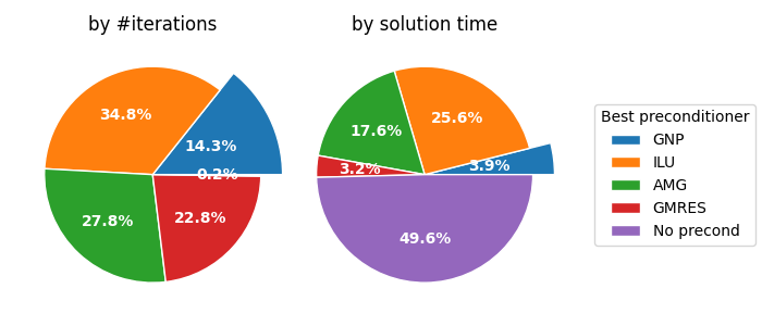
Figure 2: Percentage of problems for which each preconditioner performs the best.

For what problems does GNP perform the best? We expand the granularity of Figure 2 into Figure 3, overlaid with the size distribution and the condition-number distribution of the problems. A key finding to note is that GNP is particularly useful for ill-conditioned matrices (i.e., those with a condition number $\geq 10^{16}$). ILU is less competitive in these problems, compared with other preconditioners, possibly because it focuses on the sparsity structure, whose connection with the spectrum is less clear.

On the other hand, the matrix size does not affect much the GNP performance. One sees this more clearly when consulting Figure 7 in the appendix, which is a “proportion” version of Figure 3: the proportion of problems for which GNP performs the best is relatively flat across matrix sizes. Similarly, symmetry also does not play a distinguishing role: GNP performs the best for 8.8% of the symmetric matrices and 17.7% of the nonsymmetric matrices.

Figure 3: Breakdown of best preconditioners with respect to matrix sizes and condition numbers. The last bar on the right plot is for condition number $\geq 10^{16}$.

What does the convergence history look like with GNP? In Figure 4, we show a few examples when GNP performs the best. It is worthwhile to note that in this case, ILU fails for most of the problems, either in the construction phase or in the solution phase (more on this later). These examples indicate that the convergence of GNP either tracks that of other competitive preconditioners with a similar rate (see problems Simon/venkat25 and VDOL/kineticBatchReactor_5), or becomes significantly faster (see problems GHS_indef/bratu3d and VanVelzen/std1_Jac3). Notably, on VanVelzen/std1_Jac3, GNP uses only four iterations to reach 1e-8, while other preconditioners take 100 iterations but still cannot decrease the relative residual norm to below 1e-2.

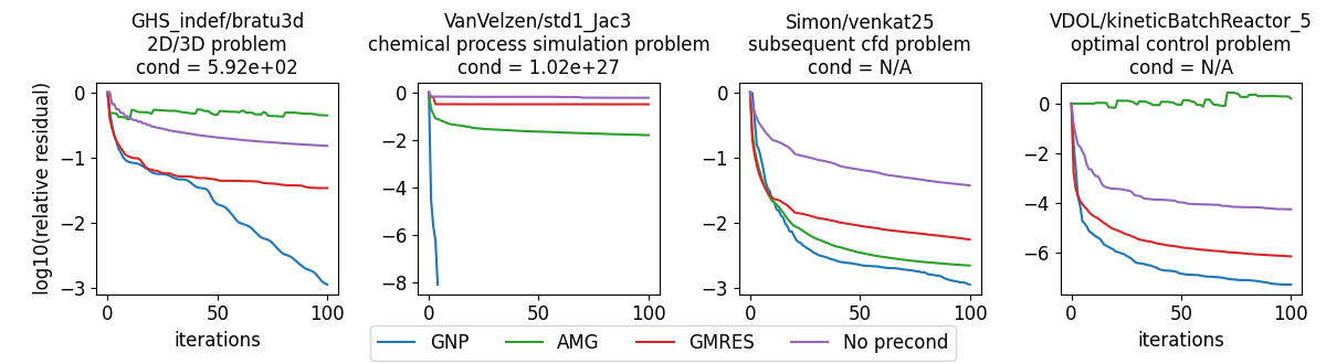
Figure 4: Example convergence histories.

We additionally plot the convergence curves with respect to time in Figure 8 in the appendix. An important finding to note is that GMRES as a preconditioner generally takes much longer time to run than GNP. This is because GMRES is bottlenecked by the orthogonalization process, shadowing the trickier cost comparison between more matrix-vector multiplications in GMRES and fewer matrix-matrix multiplications in GNP, with respect to the matrix $\mathbf{A}$.

How does the construction cost of GNP fare, compared with that of other preconditioners? GMRES does not require construction; hence, we mainly compare GNP with ILU and AMG. In Figure 5, we plot their construction times. The training time of GNP is nearly proportional to the matrix size, as expected. In contrast, the construction time of ILU and AMG is much less predictable. Even though for many of the problems, the time is only a fraction of that of GNP, there exist quite a few cases where the time is significantly longer. In the worst case, the construction of the AMG preconditioner is more than an order of magnitude more costly than that of GNP. Moreover, it is unclear when such “outliers” happen, as they do not seem to be correlated with the matrix size.

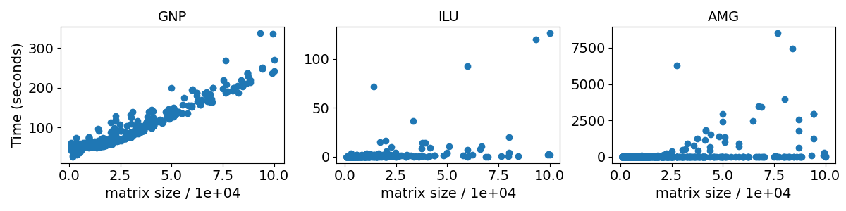
Figure 5: Preconditioner construction time.

How robust is GNP? We summarize in Table 1 the number of failures for each preconditioner. GNP and GMRES are highly robust. We see that neural network training does not cause any troubles, which is a practical advantage. In contrast, ILU fails for nearly half of the problems and AMG fails for nearly 8%. According to the error log, the common failures of ILU construction are that “(f)actor is exactly singular” and that “matrix is singular … in file ilu_dpivotL.c”, while the common failures of AMG are “array … contain(s) infs or NaNs”. Meanwhile, solution failures occur when the residual norm tracked by the QR factorization of the upper Hessenberg $\overline{\mathbf{H}}_{m}$ fails to match the actual residual norm. While these two preconditioners perform the best for the most number of problems, safeguarding their robustness on other problems remains challenging.

Table 1: Failures of preconditioners.

	GNP	ILU	AMG	GMRES
Construction failure	0 (0.00%)	348 (40.14%)	62 (7.15%)	N/A
Solution failure	1 (0.12%)	61 (07.04%)	5 (0.58%)	1 (0.12%)

Are the proposed training data generation and the scale-equivariance design necessary? In Figure 6, we compare the proposed designs versus alternatives, for both the training loss and the relative residual norm. In the comparison of training data generation, using $\mathbf{x}\sim\mathcal{N}(\mathbf{0},\mathbf{I}_{n})$ leads to lower losses, while using $\mathbf{b}\sim\mathcal{N}(\mathbf{0},\mathbf{I}_{n})$ leads to higher losses. This is expected, because the former expects similar outputs from the neural network, which is easier to train, while the latter expects drastically different outputs and makes the network difficult to train. Using $\mathbf{x}$ from the proposed mixture leads to losses lying in between. This case leads to the best preconditioning performance—more problems having lower residual norms (especially those near rtol). In other words, the proposed training data generation strikes the best balance between easiness of neural network training and goodness of the resulting preconditioner.

In the comparison of using the scaling operator $s$ versus not, we see that the training behaviors barely differ between the two choices, but using scaling admits an advantage that more problems result in lower residual norms. These observations corroborate the choices we make in the neural network design and training data generation.

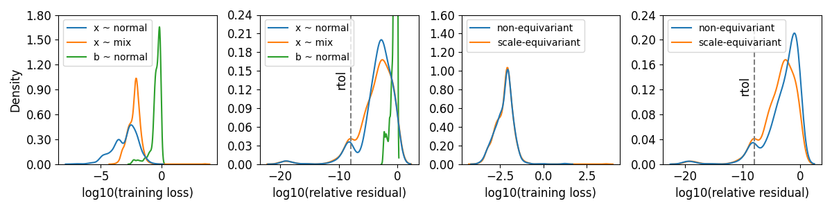
Figure 6: Left: comparison of training data generation; right: comparison of scale-equivariance.

5 Discussions and Conclusions

We have presented a GNN approach to preconditioning Krylov solvers for the solution of large, sparse linear systems. This is the first work in our knowledge to use a neural network as an approximation to the matrix inverse. Compared with traditional preconditioners, this approach is robust with predictable construction costs and is effective for highly ill-conditioned problems. We evaluate the approach on more than 800 matrices from over 20 application areas, the widest coverage in the literature.

The work can be extended in many avenues. First, an immediate follow up is the preconditioning of SPD matrices. While flexible CG was analyzed in the past [25], it is relatively fragile with respect to a large variation of the preconditioner. We speculate that a split preconditioner can work more robustly and some form of autoencoder networks better serves this purpose.

Second, while GNP is trained for an individual matrix in this work for simplicity, it is possible to extend it to a sequence of evolving matrices, such as in sequential problems or time stepping. Continual learning, which is concerned with continuously adapting a trained neural network for slowly evolving data distributions, can amortize the initial preconditioner construction cost with more and more linear systems in sequel.

Third, the GPU memory limits the size of the matrices and the complexity of the neural networks that we can experiment with. Future work can explore multi-GPU and/or distributed training of GNNs [14, 13] for scaling GNP to even larger matrices. The training for large graphs typically uses neighborhood sampling to mitigate the unique “neighborhood explosion” problem in GNNs. Some sampling approaches, such as layer-wise sampling [5], are tied to sketching the matrix product $\widehat{\mathbf{A}}\mathbf{X}$ inside the graph convolution layers (7) with certain theoretical guarantees [4].

Fourth, while we use the same set of hyperparameters for evaluation, nothing prevents problem-specific hyperparameter tuning when one works on an application, specially a challenging one where no general-purpose preconditioners work sufficiently well. We expect that this paper’s results based on a naive hyperparameter setting can be quickly improved by the community. Needless to say, improving the neural network architecture can push the success of GNP much farther.

Appendix A Proofs

Proof of Theorem 1.

Write $\|\mathbf{r}_{m}\|_{2}\leq\|\widetilde{\mathbf{r}}_{m}\|_{2}+\|\mathbf{r}_{m}-\widetilde{\mathbf{r}}_{m}\|_{2}$. It is well known that

$$\|\widetilde{\mathbf{r}}_{m}\|_{2}\leq\kappa_{2}(\mathbf{X})\epsilon^{(m)}(\bm{\Lambda})\|\mathbf{r}_{0}\|_{2};$$

see, e.g., [31, Proposition 6.32]. On the other hand, because $\mathbf{r}_{m}=\mathbf{r}_{0}-\mathbf{A}\mathbf{Z}_{m}\mathbf{y}_{m}$ where $\mathbf{y}_{m}$ minimizes $\|\mathbf{r}_{0}-\mathbf{A}\mathbf{Z}_{m}\mathbf{y}\|_{2}$, we have $\mathbf{r}_{m}=\mathbf{r}_{0}-(\mathbf{A}\mathbf{Z}_{m})(\mathbf{A}\mathbf{Z}_{m})^{+}\mathbf{r}_{0}=\mathbf{r}_{0}-\mathbf{Q}_{m}\mathbf{Q}_{m}^{\top}\mathbf{r}_{0}$. Therefore, $\|\mathbf{r}_{m}-\widetilde{\mathbf{r}}_{m}\|_{2}=\|\mathbf{Q}_{m}\mathbf{Q}_{m}^{\top}\mathbf{r}_{0}-\widetilde{\mathbf{Q}}_{m}\widetilde{\mathbf{Q}}_{m}^{\top}\mathbf{r}_{0}\|_{2}\leq\|\mathbf{Q}_{m}\mathbf{Q}_{m}^{\top}-\widetilde{\mathbf{Q}}_{m}\widetilde{\mathbf{Q}}_{m}^{\top}\|_{2}\|\mathbf{r}_{0}\|_{2}$. ∎

Proof of Corollary 2.

By taking $\widetilde{\mathbf{M}}=\mathbf{A}^{-1}\mathbf{V}_{n}\mathbf{H}_{n}\mathbf{V}_{n}^{\top}$ and noting that $\mathbf{V}_{n}^{\top}=\mathbf{V}_{n}^{-1}$, we have

$$(\mathbf{V}_{n}\mathbf{Y})^{-1}\mathbf{A}\widetilde{\mathbf{M}}(\mathbf{V}_{n}\mathbf{Y})=\operatorname{diag}(\sigma_{1},\ldots,\sigma_{n}).$$

Then, following Theorem 1, $\|\mathbf{r}_{m}\|_{2}\leq\kappa_{2}(\mathbf{V}_{n}\mathbf{Y})\epsilon^{(m)}(\bm{\Sigma})\|\mathbf{r}_{0}\|_{2}$. We conclude the proof by noting that $\kappa_{2}(\mathbf{V}_{n}\mathbf{Y})=\kappa_{2}(\mathbf{Y})$. ∎

Appendix B Additional Experiment Results

In Figure 7, we plot the proportion of problems for which each preconditioner performs the best, for different matrix sizes and condition numbers. This figure is a counterpart of Figure 3. The main observation is that the proportion of problems for which GNP performs the best is relatively flat across matrix sizes. Meanwhile, the right plot shows that GNP is particularly useful for ill-conditioned problems.

Figure 7: Proportion of problems for which each preconditioner performs the best, for different matrix sizes and condition numbers. The last bar on the right plot is for condition number $\geq 10^{16}$. Note that not every matrix has a known condition number.

In Figure 8, we show the convergence histories of the systems appearing in Figure 4, with respect to both iteration counts and time. We also plot the training curves. The short solution time of GNP is notable, especially when compared with the solution time of GMRES as a preconditioner. The training loss generally stays on the level of 1e-2 to 1e-3. For some problems (e.g., VanVelzen_std1_Jac3), training does not seem to progress well, but the training loss is already at a satisfactory point in the first place, and hence the preconditioner can be rather effective. We speculate that this behavior is caused by the favorable architectural inductive bias in the GNN.

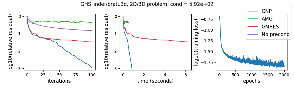
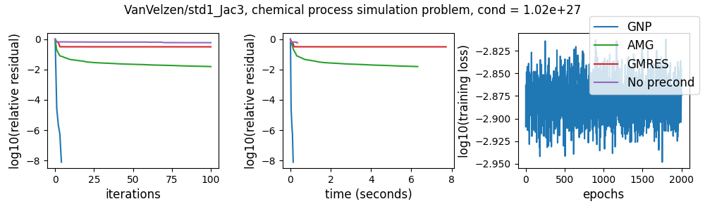
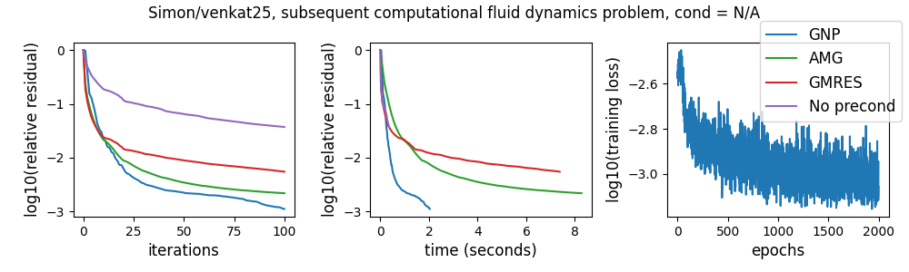
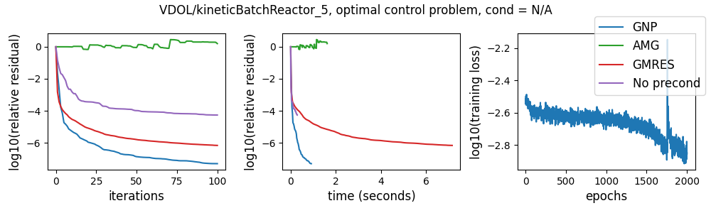
Figure 8: Convergence of the linear system solutions and training history of the preconditioners, for the matrices shown in Figure 4.

References

- [1] Nathan Bell, Luke N. Olson, Jacob Schroder, and Ben Southworth. PyAMG: Algebraic multigrid solvers in python. Journal of Open Source Software, 8(87):5495, 2023.
- [2] Rishi Bommasani et al. On the opportunities and risks of foundation models. Preprint arXiv:2108.07258, 2021.
- [3] Maria Bånkestad, Jennifer Andersson, Sebastian Mair, and Jens Sjölund. Ising on the graph: Task-specific graph subsampling via the Ising model. Preprint arXiv:2402.10206, 2024.
- [4] Jie Chen and Ronny Luss. Stochastic gradient descent with biased but consistent gradient estimators. Preprint arXiv:1807.11880, 2018.
- [5] Jie Chen, Tengfei Ma, and Cao Xiao. FastGCN: Fast learning with graph convolutional networks via importance sampling. In ICLR, 2018.
- [6] Jie Chen, Lois Curfman McInnes, and Hong Zhang. Analysis and practical use of flexible BiCGStab. Journal of Scientific Computing, 68(2):803–825, 2016.
- [7] Edmond Chow and Yousef Saad. Approximate inverse preconditioners via sparse-sparse iterations. SIAM Journal on Scientific Computing, 19(3):995–1023, 1998.
- [8] Timothy A. Davis and Yifan Hu. The university of Florida sparse matrix collection. ACM Trans. Math. Softw., 38(1):1–25, 2011.
- [9] S. Gerschgorin. Über die abgrenzung der eigenwerte einer matrix. Izv. Akad. Nauk. USSR Otd. Fiz.-Mat. Nauk, 6:749–754, 1931.
- [10] William L. Hamilton, Rex Ying, and Jure Leskovec. Inductive representation learning on large graphs. In NIPS, 2017.
- [11] Paul Häusner, Ozan Öktem, and Jens Sjölund. Neural incomplete factorization: learning preconditioners for the conjugate gradient method. Preprint arXiv:2305.16368, 2023.
- [12] Kurt Hornik, Maxwell Stinchcombe, and Halbert White. Multilayer feedforward networks are universal approximators. Neural Networks, 2(5):359–366, 1989.
- [13] Tim Kaler, Alexandros-Stavros Iliopoulos, Philip Murzynowski, Tao B. Schardl, Charles E. Leiserson, and Jie Chen. Communication-efficient graph neural networks with probabilistic neighborhood expansion analysis and caching. In MLSys, 2023.
- [14] Tim Kaler, Nickolas Stathas, Anne Ouyang, Alexandros-Stavros Iliopoulos, Tao B. Schardl, Charles E. Leiserson, and Jie Chen. Accelerating training and inference of graph neural networks with fast sampling and pipelining. In MLSys, 2022.
- [15] Diederik P. Kingma and Jimmy Ba. Adam: A method for stochastic optimization. In ICLR, 2015.
- [16] Thomas N. Kipf and Max Welling. Semi-supervised classification with graph convolutional networks. In ICLR, 2017.
- [17] Nikola Kovachki, Zongyi Li, Burigede Liu, Kamyar Azizzadenesheli, Kaushik Bhattacharya, Andrew Stuart, and Anima Anandkumar. Neural operator: Learning maps between function spaces. Journal of Machine Learning Research, 23:1–97, 2022.
- [18] Xiaoye S. Li. An overview of SuperLU: Algorithms, implementation, and user interface. ACM Trans. Mathematical Software, 31(3):302–325, 2005.
- [19] Xiaoye S. Li and Meiyue Shao. A supernodal approach to incomplete LU factorization with partial pivoting. ACM Trans. Mathematical Software, 37(4), 2010.
- [20] Yichen Li, Peter Yichen Chen, Tao Du, and Wojciech Matusik. Learning preconditioner for conjugate gradient PDE solvers. In ICML, 2023.
- [21] Zongyi Li, Nikola Kovachki, Kamyar Azizzadenesheli, Burigede Liu, Kaushik Bhattacharya, Andrew Stuart, and Anima Anandkumar. Neural operator: Graph kernel network for partial differential equations. Preprint arXiv:2003.03485, 2020.
- [22] Zongyi Li, Nikola Kovachki, Kamyar Azizzadenesheli, Burigede Liu, Kaushik Bhattacharya, Andrew Stuart, and Anima Anandkumar. Fourier neural operator for parametric partial differential equations. In ICLR, 2021.
- [23] Lu Lu, Pengzhan Jin, and George Em Karniadakis. Learning nonlinear operators via DeepONet based on the universal approximation theorem of operators. Nature Machine Intelligence, 3:218–229, 2021.
- [24] Ronald B. Morgan. GMRES with deflated restarting. SIAM Journal on Scientific Computing, 24(1):20–37, 2002.
- [25] Yvan Notay. Flexible conjugate gradients. SIAM Journal on Scientific Computing, 22(4):1444–1460, 2000.
- [26] M. Raissi, P. Perdikaris, and G.E. Karniadakis. Physics-informed neural networks: A deep learning framework for solving forward and inverse problems involving nonlinear partial differential equations. Journal of Computational Physics, 378:686–707, 2019.
- [27] J. W. Ruge and K. Stüben. Algebraic multigrid. In Stephen F. McCormick, editor, Multigrid Methods, Frontiers in Applied Mathematics, chapter 4. SIAM, 1987.
- [28] Y. Saad. ILUT: A dual threshold incomplete LU factorization. Numerical Linear Algebra with Applications, 1(4):387–402, 1994.
- [29] Youcef Saad. A flexible inner-outer preconditioned GMRES algorithm. SIAM Journal on Scientific Computing, 14(2):461–469, 1993.
- [30] Youcef Saad and Martin H. Schultz. GMRES: A generalized minimal residual algorithm for solving nonsymmetric linear systems. SIAM Journal on Scientific and Statistical Computing, 7(3):856–869, 1986.
- [31] Yousef Saad. Iterative Methods for Sparse Linear Systems. Society for Industrial and Applied Mathematics, second edition, 2003.
- [32] Petar Velic̆ković, Guillem Cucurull, Arantxa Casanova, Adriana Romero, Pietro Liò, and Yoshua Bengio. Graph attention networks. In ICLR, 2018.
- [33] Zonghan Wu, Shirui Pan, Fengwen Chen, Guodong Long, Chengqi Zhang, and Philip S. Yu. A comprehensive survey on graph neural networks. IEEE Transactions on Neural Networks and Learning Systems, 32(1):4–24, 2021.
- [34] Keyulu Xu, Weihua Hu, Jure Leskovec, and Stefanie Jegelka. How powerful are graph neural networks? In ICLR, 2019.
- [35] Jie Zhou, Ganqu Cui, Shengding Hu, Zhengyan Zhang, Cheng Yang, Zhiyuan Liu, Lifeng Wang, Changcheng Li, and Maosong Sun. Graph neural networks: A review of methods and applications. AI Open, 1:57–81, 2020.