MagR: Weight Magnitude Reduction for Enhancing Post-Training Quantization
Abstract
In this paper, we present a simple optimization-based preprocessing technique called Weight Magnitude Reduction (MagR) to improve the performance of post-training quantization. For each linear layer, we adjust the pre-trained floating-point weights by solving an -regularized optimization problem. This process greatly diminishes the maximum magnitude of the weights and smooths out outliers, while preserving the layer’s output. The preprocessed weights are centered more towards zero, which facilitates the subsequent quantization process. To implement MagR, we address the -regularization by employing an efficient proximal gradient descent algorithm. Unlike existing preprocessing methods that involve linear transformations and subsequent post-processing steps, which can introduce significant overhead at inference time, MagR functions as a non-linear transformation, eliminating the need for any additional post-processing. This ensures that MagR introduces no overhead whatsoever during inference. Our experiments demonstrate that MagR achieves state-of-the-art performance on the Llama family of models. For example, we achieve a Wikitext2 perplexity of 5.95 on the LLaMA2-70B model for per-channel INT2 weight quantization without incurring any inference overhead.
1 Introduction
Large language models (LLMs) have achieved outstanding performance across a broad range of applications, demonstrating remarkable success. However, their unprecedented model size has led to many computation operations and substantial memory footprints, becoming significant barriers to their practical deployment and adoption in production environments. Accordingly, it is highly desirable to develop efficient model compression techniques for LLMs so they can be more widely deployed in resource-limited scenarios. Among the various techniques to compress and accelerate deep neural networks (DNNs), low-precision quantization has proven to be highly effective across numerous application domains and is widely adopted for accelerating DNNs. For LLMs, the inference runtime is dominated by the token generation process, where output tokens are produced sequentially, one at a time. This process is known to be memory bandwidth bound aminabadi2022deepspeed ; kim2023stack . As a result, the quantization of LLMs has primarily focused on reducing the bit-width of model weights, with the dual goals of lowering the model’s footprint to enable deployment on resource-constrained devices and decreasing the memory bandwidth requirements to improve computational efficiency and accelerate inference.
The enormous computational demands for pre-training and fine-tuning Large Language Models (LLMs) have led to the emergence of Post-Training Quantization (PTQ) behdin2023quantease ; frantar2022optimal ; li2021brecq ; lin2023bit ; maly2023simple ; nagel2019data ; wang2022deep ; wei2022qdrop ; zhang2024comq ; zhang2023post as a promising solution for quantizing these models. Unlike Quantization Aware Training (QAT) cai2017deep ; choi2018pact ; hubara2018quantized ; rastegari2016xnor ; yin2019blended , which is designed to minimize a global training loss for quantization parameters, PTQ directly applies low-precision calibration to a pre-trained full-precision model using a minimal set of calibration samples. By aiming to identify an optimal quantized model locally through the minimization of a simplified surrogate loss, PTQ offers computational savings and resource efficiency compared to QAT. However, PTQ often lags behind QAT in accuracy, particularly for ultra-low precision lower than 4 bit. Thus, it remains an open problem to achieve an improved balance between cost and performance for PTQ-based approaches.
Motivation. To achieve state-of-the-art performance, the latest advances in PTQ chee2024quip ; lin2023awq ; ma2024affinequant ; shao2023omniquant ; wei2023outlier have proposed applying a linear transformation to process the pre-trained weights within a linear layer. This strategy of linear transformation aims to make the weights more suitable for the subsequent quantization procedure by reducing their magnitudes and suppressing outliers. In a nutshell, given the features and weights , one constructs some matrix such that is better conditioned than in terms of being quantization-friendly. Such designs of include diagonal matrix (so-called channel-wise scaling) shao2023omniquant ; wei2023outlier as in AWQ lin2023awq and random orthogonal matrix as in QuIP chee2024quip . Then, quantization is performed on instead of the original weights . To preserve the layer’s output, however, the inverse transformation has to be in turn applied to the features , namely,
with being the quantized weights. PTQ done this way requires modifications on the original neural architecture, which involves additional computations of and extra memory storage for at inference time. As a result, these steps introduce overhead that offsets the benefits provided by quantization. This raises a natural question:
Can we effectively process the weights at the preprocessing stage to facilitate quantization without introducing inference overhead?
To address this problem, we propose a simple optimization-based technique called Weight Magnitude Reduction (MagR). MagR functions as a non-linear transformation on weights without altering the original layer-wise features. The optimization program is designed to find new weights with minimal maximum magnitude, i.e., the norm, while preserving the layer’s outputs.
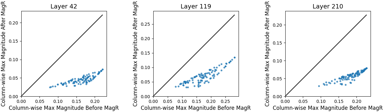
Contributions. We propose a non-linear approach, MagR, based on -regularization, to reduce the quantization scale, facilitating subsequent weight quantization while requiring no post-processing or inference overhead. See Figure 1 for comparing weight magnitudes before and after applying MagR. To efficiently solve the resulting -regularization problem, we develop a proximal gradient descent algorithm which involves computing -ball projection during the iterations. Our results on INT weight-quantization demonstrate that MagR can significantly boost accuracy in the sub-4bit regime when combined with fast gradient-free methods for layer-wise PTQ, such as rounding-to-nearest (RTN) nagel2020up and OPTQ frantar2022optq . This approach achieves performance for weight quantization comparable to state-of-the-art PTQ methods on natural language processing (NLP) tasks, including gradient-based methods using block-wise reconstruction.
2 Related Work
Recently, as the sizes of language models are exploding, there has been growing interest in developing post-training quantization (PTQ) methods chee2024quip ; frantar2022optq ; lin2023awq ; ma2024affinequant ; shao2023omniquant ; yao2024exploring ; xiao2023smoothquant for large-scale AI models like large language models (LLMs) to reduce the model sizes and accelerate inference by representing weight matrices in low precision. PTQ methods directly find the low-precision representation of the model without re-training, thereby preferred by extreme large-scale AI models. The OPTQ frantar2022optq uses approximate second-order information to calibrate the quantization. The method successfully compresses LLMs into 3 or 4 bits and can achieve reasonable accuracy in 2 bits. Researchers have found that the extreme values and the distribution of the weight entries highly affect the quantization errors and the quantized model quality. The original weight can be converted into a more quantization-friendly one by linear transformations. The approach can significantly reduce the quantization errors while bringing more time overhead during inference because of the linear transformation. OmniQuant shao2023omniquant proposes learnable weight clippings and equivalent transformations to avoid the influence of extreme values. AWQ lin2023awq searches for the most significant entries in the weight by looking at the activation and selects the scales that protect these entries. SmoothQuant xiao2023smoothquant passes the difficulty in activation quantization to weights by an equivalent linear transformation. QuIP chee2024quip and AffineQuant ma2024affinequant apply a linear transformation before quantization to make the transformed weight quantization-friendly. These approaches achieve high performance for extreme bits, like 2 bits, but introduce additional inference overhead though the transformation is carefully designed to be efficient. OmniQuant shao2023omniquant and AffineQuant ma2024affinequant can be adopted for weight-activation quantization by considering the activations in the proposed methods. The work yao2024exploring introduces a low-rank compensation method on top of other quantization methods, which employs low-rank matrices to reduce quantization errors with a minimal increase in model size.
3 Background
First, we clarify the mathematical notations that will be used throughout this paper:
Notations. We denote vectors by bold small letters and matrices by bold capital ones. For a positive integer , denotes the set containing all positive integers up to . For any two vectors , is the inner product. We denote by the Euclidean norm; is the -norm; is the -norm. For any matrix , is the transpose. Its Frobenius norm is given by . Moreover, for vectors and , denotes the Hadamard or element-wise product, and likewise for two matrices.
Layerwise PTQ. Post-training quantization via layerwise reconstruction calls for solving a least squares problem with a discrete constraint. For the pre-trained weights within a linear layer, we aim to find the quantized weights that minimize the following function
| (1) |
where is the feature matrix associated with a batch of calibration data consisting of samples stacked together, and each data sample is represented by an sub-matrix. is an appropriate set of all feasible quantized weights.
The most straightforward PTQ technique, known as RTN, involves directly rounding the weight matrix without utilizing any additional data. An improvement over RTN was introduced by AWQ lin2023awq , which enhances the quantization process by incorporating channel-wise scaling on . Thanks to the simplicity of the layer-wise formulation (1), several efficient gradient-free algorithms behdin2023quantease ; frantar2022optq ; zhang2024comq ; zhang2023post have been recently proposed to address layer-wise quantization, including OPTQ. Built on top of OPTQ, QuIP subjects and to random orthogonal transformations to produce “incoherent" weight and Hessian matrices, leading to superior accuracy with sub-4bit quantization. However, this advantage comes with a trade-off; during inference, QuIP requires random orthogonal transformations on the feature inputs of linear layers, rendering noticeably slower throughput compared to OPTQ.
Uniform Quantizer. Given a set of points , the commonly-used (asymmetric) uniform quantizer choi2018pact defines the quantization step and zero-point , and it quantizes onto the scaled integer grids as follows:
In per-channel (or per-group) PTQ, the quantization step is conventionally calculated based on the channel-wise (or group-wise, respectively) minimum and maximum values of the pre-trained weights , as defined above, and remains constant throughout the quantization procedure.
4 The Proposed Method
In this section, we present the Weight Magnitude Reduction (MagR) method based on -norm regularization. which is performed immediately prior to the quantization step within each linear layer.
4.1 Rank-Deficient Feature Matrix
To illustrate the idea behind the proposed MagR method, let us consider a pre-trained weight vector of a linear layer and the associated feature input matrix . MagR leverages the fact that the feature matrix across all layers of LLMs is approximately rank-deficient. Specifically, if is rank-deficient, the linear system modeling the layer’s output, with variables , generally has infinitely many solutions. That is, for any in the non-trivial kernel space of , we have that preserves the layer’s output. Among all solutions, MagR aims to identify the weight vector with the smallest extreme value in magnitude.
In chee2024quip , the authors empirically observed that the Hessian matrix is approximately low-rank across all layers in open pre-trained (OPT) models zhang2022opt . Specifically, it was shown that the fraction of eigenvalues of that satisfy , i.e. approximate fraction rank, is much smaller than 1. Here we further examined the feature matrix of LLaMA models touvron2023llama ; touvron2023llama2 . Our approximate fraction rank of the feature matrix is defined as the fraction of singular values of such that . It is worth noting that our definition of being rank-deficient is more stringent compared to the one used in chee2024quip . Indeed, if a singular value of obeys , then the corresponding eigenvalue of gives . Table 1 illustrates that all feature matrices extracted from LLaMA models are rank-deficient according to this definition.
| Model | Min | Max | Mean | 25% Percentile | 75% Percentile |
|---|---|---|---|---|---|
| LLaMA1-7B | 0.2 | 99.07 | 70.41 | 65.09 | 81.80 |
| LLaMA1-13B | 1.42 | 99.90 | 83.85 | 75.07 | 96.71 |
| LLaMA1-30B | 0.73 | 99.85 | 84.40 | 79.76 | 99.46 |
| LLaMA1-65B | 1.17 | 99.90 | 83.11 | 82.76 | 98.71 |
| LLaMA2-7B | 0.1 | 99.95 | 76.83 | 67.71 | 91.02 |
| LLaMA2-13B | 0.44 | 99.76 | 78.30 | 66.54 | 98.58 |
| LLaMA2-70B | 0.1 | 99.71 | 81.55 | 74.90 | 99.56 |
4.2 MagR via -Regularization
Let us consider the quantization of a weight vector for simplicity. Given pre-trained weight vector , we would like to find a new set of weights with the smallest maximum magnitude, such that the layer output is preserved up to a small error , i.e.,
To efficiently implement MagR, we consider the following mathematically equivalent -regularization problem instead:
| (2) |
where serves as the regularization parameter, balancing fidelity against the regularizer. To maintain the output of the layer, should typically be set to a small value.
Proximal Gradient Descent. Note that -norm is a convex but non-differentiable function. In theory, the optimization problem (2) can be simply solved by a subgradient algorithm, but it is significantly slower than the more sophisticated proximal gradient algorithm which matches the convergence rate of standard gradient descent.
With the step size , proximal gradient descent parikh2014proximal takes the following iteration:
| (3) |
where with the scalar is the (scaled) proximal operator of -norm function, defined as
To ensure the convergence of (3), it is sufficient to choose the step size
where is the maximum eigenvalue of .
Proximal Operator of -Norm. It remains to determine the proximal operator of -norm. It turns out we can compute it by leveraging the celebrated Moreau decomposition moreau1962decomposition ; parikh2014proximal : for any ,
| (4) |
That is, computing the proximal operator of norm amounts to evaluating the projection onto ball, which is defined as
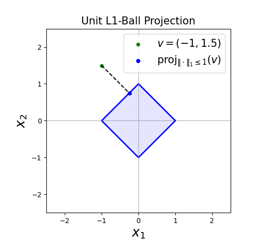
Fortunately, computing projection onto the ball is an established task, and there are several efficient algorithms available. For example, see condat2016fast and the references therein. Here we adopted a simple algorithm of time complexity as in duchi2008efficient , which supports parallelizable or vectorized implementation for the projections of a batch of weight vectors, i.e., a weight matrix, as will be described in the next subsection. The implementation mainly involves sorting and soft-thresholding yin2008bregman ; see Algorithm 3 in Appendix A.1 for the details.
MagR for Weight Matrix. In practical implementation of MagR, we preprocess the entire weight matrix within each linear layer. For per-channel quantization (or per-column quantization in our setting), the penalty is imposed column-wise on the weight matrix to reduce the quantization scale of each channel. That is, MagR amounts to solving
In this case, we take the following iteration:
where the proximal operator and the corresponding projection in (4) are applied column-wise to the matrix input. Hereby we summarize MagR for processing one linear layer in Algorithm 1 with the column-wise -ball projection for matrix input as detailed in Algorithm 2.
Input: Pre-trained weight matrix ; Hessian matrix ; max iteration number ; step size ; penalty parameter .
Output: Preprocessed weights .
Input: Matrix ; the radius of ball, .
Output: such that all columns , .
MagR for Per-Group Quantization. By using more float scaling factors, per-group quantization becomes a preferred strategy for mitigating accuracy loss at extremely low bit-widths. In this approach, a weight vector is segmented into groups of weights, each containing elements, with all weights within a group sharing a common scaling factor for quantization. Here, per-group MagR applies an penalty to each vector of grouped weights. Consequently, the -ball projection is independently performed on these vectors, while maintaining the gradient descent step unchanged. We note that the group-wise -ball projection can be easily done using Algorithm 2, with an additional reshaping of the input into .
5 Experiments
Overview. We tested the proposed MagR for INT4, INT3, and INT2 weight quantization. In our notations, the weight and activation bits are denoted by ‘W’ and ‘A’, respectively. Additionally, we implemented group-wise weight quantization with the group size denoted by ‘g’. For example, W2A16g128 signifies INT2 weight and FP16 activation (i.e., INT2 weight-only quantization) with a group size of 128.
We employed our MagR processing approach on top of the two gradient-free PTQ methods, RTN and OPTQ frantar2022optq , to quantize the LLaMA1 (7B-65B) touvron2023llama and LLaMA2 (7B-70B) touvron2023llama2 model families. By applying MagR on top of RTN (MagR+RTN), we achieved better results than AWQ lin2023awq for per-channel INT3 and INT4 weight quantization. Additionally, MagR combined with OPTQ (MagR+OPTQ) achieved state-of-the-art performance for INT3 and INT4 qunatization. To enhance the per-channel INT2 quantization, we ran 30 additional iterations of coordinate descent algorithm zhang2024comq on top of OPTQ, which we denote by MagR+OPTQ†. It turns out MagR+OPTQ† is superior to both Omniquant shao2023omniquant and QuIP chee2024quip in terms of perplexity (Table 2), and falls just short of QuIP in zero-shot tasks for 13B and 70B models (Table 3). Note that QuIP uses random orthogonal transformations (so-called Incoherence Processing) to process both the weights and features, resulting in slower throughput than OPTQ. In contrast, MagR-based method does not introduce any overhead whatsoever compared with OPTQ.
In conclusion, our MagR-based PTQ method is intuitive yet effective in compressing models into extreme bit-widths, while maintaining performance without introducing any inference overhead.
Datasets and Evaluation. Following the previous work frantar2022optq ; lin2023awq ; shao2023omniquant , we evaluate the quantized model on language generation tasks on WikiText2 merity2016pointer and C4 raffel2020exploring . Additionally, we test its performance on zero-shot tasks, including PIQA bisk2020piqa , ARC (Easy and Challenge) clark2018think , and Winogrande sakaguchi2021winogrande . For the language generation experiments, our implement is based on the OPTQ’s frantar2022optq repository, which is built using PyTorch. For executing all zero-shot tasks, we adhere to the lm-eval-harness eval-harness .
Baseline: For the language generation task, we compare our method with RTN, OPTQ frantar2022optq , AWQ lin2023awq and OmniQuant shao2023omniquant on LLaMA1 and LLaMA2 models. In addition to the aforementioned methods, we also conduct a comparison with QuIP chee2024quip on the LLaMA2-70B model. In the zero-shot task, we focus on four individual tasks and compare the average accuracy across all four tasks with Omniquant shao2023omniquant .
Implementation details. We utilized the HuggingFace implementations of the LLaMA1 and LLaMA2 models and perform quantization on a single NVIDIA A100 GPU with 80GB of memory. Following the OPTQ method, we load one block consisting of 7 linear layers into GPU memory at a time. In line with previous work chee2024quip ; frantar2022optq , the input matrix is obtained by propagating the calibration data through the quantized layers.
The choice of parameters. To ensure that the MagR-processed layer output is faithful to the original , we need to use a tiny penalty parameter in (2). For per-channel quantization, was fixed to be in our experiments, but we did find that setting it to a smaller value of or can sometimes slightly improve the perplexity (with a relative change of in ppl). Similarly for per-group quantization, we set to , while reducing it to or could sometimes also slightly improve the perplexity.
Furthermore, we used a multiplicative scalar to decay the standard quantization step (or equivalently, the quantization scale) of the quantizer. In other words, our . It has been shown in existing works li2016ternary ; rastegari2016xnor that, optimal quantization step for binary or ternary quantization yielding the minimum quantization error is not given by . Shrinking at low bit-width results in a more clustered quantization grid lattice that fits the weights better, which leads to a smaller overall error. In general, is positively correlated with the bit-width used. For per-channel quantization, the best on INT2 quantization, whereas the empirically optimal is around for INT3 quantization. As for INT4, is simply set to 1, that is, we used the standard quantization step. In addition, for per-group quantization, we chose for both INT2 and INT3 quantization. We observed that this refinement on the quantization step significantly improves the performance of the PTQ method. In addition, the iteration number in Algorithm 1 was set to across all the experiments.
| Datasets | Wikitext2 | C4 | |||||
|---|---|---|---|---|---|---|---|
| LLaMA / PPL | 2-7B | 2-13B | 2-70B | 2-7B | 2-13B | 2-70B | |
| FP16 | Baseline | 5.47 | 4.88 | 3.31 | 6.97 | 6.46 | 5.52 |
| W2A16 | OPTQ | 7.7e3 | 2.1e3 | 77.95 | NAN | 323.12 | 48.82 |
| OmniQuant | 37.37 | 17.21 | 7.81 | 90.64 | 26.76 | 12.28 | |
| QuIP | - | - | 6.33 | - | - | 8.94 | |
| MagR+OPTQ† | 16.73 | 11.14 | 5.95 | 23.73 | 14.45 | 8.53 | |
| W2A16 g128 | OPTQ | 36.77 | 28.14 | - | 33.70 | 20.97 | - |
| OmniQuant | 11.06 | 8.26 | 6.55 | 15.02 | 11.05 | 8.52 | |
| MagR+OPTQ | 9.94 | 7.63 | 5.52 | 14.08 | 10.57 | 8.05 | |
| W3A16 | RTN | 539.48 | 10.68 | 7.52 | 402.35 | 12.51 | 10.02 |
| OPTQ | 8.37 | 6.44 | 4.82 | 9.81 | 8.02 | 6.57 | |
| AWQ | 24.00 | 10.45 | - | 23.85 | 13.07 | - | |
| OmniQuant | 6.58 | 5.58 | 3.92 | 8.65 | 7.44 | 6.06 | |
| QuIP | - | - | 3.85 | - | - | 6.14 | |
| MagR+RTN | 8.66 | 6.55 | 4.64 | 10.78 | 8.26 | 6.77 | |
| MagR+OPTQ | 6.41 | 5.41 | 3.82 | 8.23 | 7.19 | 6.03 | |
| W3A16 g128 | RTN | 6.66 | 5.51 | 3.97 | 8.40 | 7.18 | 6.02 |
| OPTQ | 6.29 | 5.42 | 3.85 | 7.89 | 7.00 | 5.85 | |
| AWQ | 6.24 | 5.32 | - | 7.84 | 6.94 | - | |
| OmniQuant | 6.03 | 5.28 | 3.78 | 7.75 | 6.98 | 5.85 | |
| MagR+RTN | 6.46 | 5.45 | 3.95 | 8.22 | 7.12 | 6.00 | |
| MagR+OPTQ | 6.00 | 5.23 | 3.71 | 7.77 | 6.93 | 5.84 | |
| W4A16 | RTN | 6.11 | 5.20 | 3.67 | 7.71 | 6.83 | 5.79 |
| OPTQ | 5.83 | 5.13 | 3.58 | 7.37 | 6.70 | 5.67 | |
| AWQ | 6.15 | 5.12 | - | 7.68 | 6.74 | - | |
| OmniQuant | 5.74 | 5.02 | 3.47 | 7.35 | 6.65 | 5.65 | |
| QuIP | - | - | 3.53 | - | - | 5.87 | |
| MagR+RTN | 5.91 | 5.17 | 3.58 | 7.52 | 6.81 | 5.72 | |
| MagR+OPTQ | 5.70 | 4.97 | 3.44 | 7.28 | 6.63 | 5.63 | |
5.1 Language Generation
We concentrate our analysis on perplexity-based tasks. The results for the LLaMA2 family with context length of 2048, are elaborated in Table 2, while those for LLaMA1 are provided in Appendix Table 5. As evidenced by the tables, the MagR preprocessing consistently improve the performance of the baselines RTN and OPTQ. Moreover, MagR+OPTQ consistently outperforms most baseline across the LLaMA family models for both per-channel and per-group weight quantization. Particularly, for INT2, MagR+OPTQ† performs 30 additional coordinate descent (CD) iterations on top of OPTQ to refine the solution, surpassing all baselines.
Furthermore, MagR+RTN achieves performance comparable to OPTQ. Notably, it outperforms AWQ by a significant margin in INT3 quantization, implying that MagR proves more effective as a preprocessing method compared to channel-wise scaling.
| LLaMA2 / Acc | WBits | Method | ARC-C | ARC-E | PIQA | Winogrande | Avg. |
|---|---|---|---|---|---|---|---|
| LLaMA2-7B | FP16 | - | 40.0 | 69.3 | 78.5 | 67.3 | 63.8 |
| 4 | OmniQuant | 37.9 | 67.8 | 77.1 | 67.0 | 62.5 | |
| 4 | MagR+OPTQ | 39.3 | 68.4 | 78 | 66.5 | 63.1 | |
| 3 | OmniQuant | 35.3 | 62.6 | 73.6 | 63.6 | 58.8 | |
| 3 | MagR+OPTQ | 34.6 | 62 | 74.7 | 63 | 58.6 | |
| 2 | OmniQuant | 21.6 | 35.2 | 57.5 | 51.5 | 41.5 | |
| 2 | QuIP | 19.4 | 26.0 | 54.6 | 51.8 | 37.5 | |
| 2 | MagR+OPTQ† | 22.0 | 36.7 | 59.8 | 51.1 | 42.4 | |
| LLaMA2-13B | FP16 | - | 45.6 | 73.3 | 79.10 | 69.6 | 65.5 |
| 4 | OmniQuant | 43.1 | 70.2 | 78.4 | 67.8 | 64.9 | |
| 4 | QuIP | 44.9 | 73.3 | 79 | 69.7 | 66.7 | |
| 4 | MagR+OPTQ | 44.2 | 72.0 | 78.0 | 68.6 | 65.7 | |
| 3 | OmniQuant | 42.0 | 69.0 | 77.7 | 65.9 | 63.7 | |
| 3 | QuIP | 41.5 | 70.4 | 76.9 | 69.9 | 64.7 | |
| 3 | MagR+OPTQ | 42.2 | 69.0 | 77.7 | 66.5 | 63.9 | |
| 2 | OmniQuant | 23.0 | 44.4 | 62.6 | 52.6 | 45.7 | |
| 2 | QuIP | 23.5 | 45.2 | 62.0 | 52.8 | 45.9 | |
| 2 | MagR+OPTQ† | 23.2 | 44.3 | 62.4 | 52.1 | 45.5 | |
| LLaMA2-70B | FP16 | - | 51.1 | 77.7 | 81.1 | 77.0 | 71.7 |
| 4 | OmniQuant | 49.8 | 77.9 | 80.7 | 75.8 | 71.1 | |
| 4 | QuIP | 47.0 | 74.3 | 80.3 | 76.0 | 69.4 | |
| 4 | MagR+OPTQ | 50.1 | 77.5 | 80.8 | 76.0 | 71.1 | |
| 3 | OmniQuant | 47.6 | 75.7 | 79.7 | 73.5 | 69.1 | |
| 3 | QuIP | 46.3 | 73.2 | 80.0 | 74.6 | 68.5 | |
| 3 | MagR+OPTQ | 47.7 | 76.6 | 79.4 | 75.4 | 69.8 | |
| 2 | OmniQuant | 28.7 | 55.4 | 68.8 | 53.2 | 51.5 | |
| 2 | QuIP | 34.0 | 62.2 | 74.8 | 67.5 | 59.6 | |
| 2 | MagR+OPTQ† | 35.9 | 61.3 | 74.7 | 64.8 | 59.2 |
5.2 Zero-Shot Tasks
We evaluated the performance of quantized models on several zero-shot tasks. The results are reported in Table 3. Similar to previous observations, the proposed MagR demonstrates superior performance on most models compared to OmniQuant, with a small gap compared to QuIP chee2024quip . Nonetheless, it is reasonable and commendable that our algorithm achieves results close to QuIP without introducing any inference overhead. It is possible to further improve our approach based on the insight behind QuIP chee2024quip - i.e., quantization benefits from incoherent weight and Hessian matrices. As shown in Table 3, incoherence processing often improves the quantization of large models, especially at higher compression rates (e.g., 2bits). The extension of MagR into incoherence preprocessing is left for future work.
| Method/ Model | LLaMA2-7B | LLaMA2-13B | LLaMA2-70B |
|---|---|---|---|
| RTN | 5 min | 12 min | 36 min |
| MagR+RTN | 20 min | 40 min | 4 hr |
| OPTQ | 22 min | 40 min | 4 hr |
| MagR+OPTQ | 35 min | 70 min | 7.5 hr |
| MagR+OPTQ† | 2.5 hr | 5.5 hr | 31 hr |
5.3 Runtime
We report the execution time of MagR+RTN and MagR+OPTQ on a single NVIDIA A100 GPU in Table 4. For example, it typically took 0.5-7.5 hours for MagR+OPTQ to quantize the LlaMA2 models. We note that the integration of MagR can markedly enhance the performance of the standard OPTQ frantar2022optq . It is noted that MagR+OPTQ† for INT2 weight quantization requires a longer runtime due to the additional CD iterations, extending the quantization process for LLaMA2-70B to 31 hr. It also reveals that the preprocessing overhead for quantizing the LLaMA2 models (7B-70B) amounts to approximately 15 min, 30 min, and 3.5 hr, respectively. In comparison, our total runtime is roughly half of that of the gradient-based method, OmniQuant shao2023omniquant , while achieving at least comparable results. Moreover, MagR introduces no post-processing step or overhead during inference.
6 Concluding Remarks
In this paper, we proposed MagR, based on -regularization, to significantly reduce the maximum weight magnitude of pre-trained LLMs within each layer while preserving their output. MagR is designed to enhance the accuracy of backpropagation-free PTQ methods that use layer-wise reconstruction, such as RTN and OPTQ. MagR produces a more clustered distribution of weights and leads to a smaller quantization step, thereby facilitating the subsequent PTQ task. To solve the -regularization problem, we used the classical proximal gradient descent algorithm with -ball projections, tailored to handle matrix variables efficiently. Our experiments on LLaMA family validated the effectiveness of the MagR approach, achieving the state-of-the-art performance on NLP tasks. Remarkably, unlike existing weight preprocessing techniques that require performing an inverse transformation on features during inference, MagR eliminates the need for post-processing and incurs no overhead. This renders MagR more practical for the deployment of quantized models.
Acknowledgement
This work was partially supported by NSF grants DMS-2208126, DMS-2110836, IIS-2110546, CCSS-2348046, SUNY-IBM AI Research Alliance Grant, and a start-up grant from SUNY Albany. We would also like to thank SUNY Albany for providing access to the Nvidia A100 GPUs.
References
- [1] Reza Yazdani Aminabadi, Samyam Rajbhandari, Minjia Zhang, Ammar Ahmad Awan, Cheng Li, Du Li, Elton Zheng, Jeff Rasley, Shaden Smith, Olatunji Ruwase, and Yuxiong He. Deepspeed inference: Enabling efficient inference of transformer models at unprecedented scale, 2022.
- [2] Kayhan Behdin, Ayan Acharya, Aman Gupta, Sathiya Keerthi, and Rahul Mazumder. Quantease: Optimization-based quantization for language models–an efficient and intuitive algorithm. arXiv preprint arXiv:2309.01885, 2023.
- [3] Yonatan Bisk, Rowan Zellers, Jianfeng Gao, Yejin Choi, et al. Piqa: Reasoning about physical commonsense in natural language. In Proceedings of the AAAI conference on artificial intelligence, volume 34, pages 7432–7439, 2020.
- [4] Zhaowei Cai, Xiaodong He, Jian Sun, and Nuno Vasconcelos. Deep learning with low precision by half-wave gaussian quantization. In Proceedings of the IEEE conference on computer vision and pattern recognition, pages 5918–5926, 2017.
- [5] Jerry Chee, Yaohui Cai, Volodymyr Kuleshov, and Christopher M De Sa. Quip: 2-bit quantization of large language models with guarantees. Advances in Neural Information Processing Systems, 36, 2024.
- [6] Jungwook Choi, Zhuo Wang, Swagath Venkataramani, Pierce I-Jen Chuang, Vijayalakshmi Srinivasan, and Kailash Gopalakrishnan. Pact: Parameterized clipping activation for quantized neural networks. arXiv preprint arXiv:1805.06085, 2018.
- [7] Peter Clark, Isaac Cowhey, Oren Etzioni, Tushar Khot, Ashish Sabharwal, Carissa Schoenick, and Oyvind Tafjord. Think you have solved question answering? try arc, the ai2 reasoning challenge. arXiv preprint arXiv:1803.05457, 2018.
- [8] Laurent Condat. Fast projection onto the simplex and the ball. Mathematical Programming, 158(1):575–585, 2016.
- [9] John Duchi, Shai Shalev-Shwartz, Yoram Singer, and Tushar Chandra. Efficient projections onto the l 1-ball for learning in high dimensions. In Proceedings of the 25th international conference on Machine learning, pages 272–279, 2008.
- [10] Elias Frantar and Dan Alistarh. Optimal brain compression: A framework for accurate post-training quantization and pruning. Advances in Neural Information Processing Systems, 35:4475–4488, 2022.
- [11] Elias Frantar, Saleh Ashkboos, Torsten Hoefler, and Dan Alistarh. Optq: Accurate quantization for generative pre-trained transformers. In The Eleventh International Conference on Learning Representations, 2022.
- [12] Leo Gao, Jonathan Tow, Baber Abbasi, Stella Biderman, Sid Black, Anthony DiPofi, Charles Foster, Laurence Golding, Jeffrey Hsu, Alain Le Noac’h, Haonan Li, Kyle McDonell, Niklas Muennighoff, Chris Ociepa, Jason Phang, Laria Reynolds, Hailey Schoelkopf, Aviya Skowron, Lintang Sutawika, Eric Tang, Anish Thite, Ben Wang, Kevin Wang, and Andy Zou. A framework for few-shot language model evaluation, 12 2023.
- [13] Itay Hubara, Matthieu Courbariaux, Daniel Soudry, Ran El-Yaniv, and Yoshua Bengio. Quantized neural networks: Training neural networks with low precision weights and activations. Journal of Machine Learning Research, 18(187):1–30, 2018.
- [14] Sehoon Kim, Coleman Hooper, Thanakul Wattanawong, Minwoo Kang, Ruohan Yan, Hasan Genc, Grace Dinh, Qijing Huang, Kurt Keutzer, Michael W. Mahoney, Yakun Sophia Shao, and Amir Gholami. Full stack optimization of transformer inference: a survey, 2023.
- [15] Fengfu Li, Bin Liu, Xiaoxing Wang, Bo Zhang, and Junchi Yan. Ternary weight networks. arXiv preprint arXiv:1605.04711, 2016.
- [16] Yuhang Li, Ruihao Gong, Xu Tan, Yang Yang, Peng Hu, Qi Zhang, Fengwei Yu, Wei Wang, and Shi Gu. Brecq: Pushing the limit of post-training quantization by block reconstruction. arXiv preprint arXiv:2102.05426, 2021.
- [17] Chen Lin, Bo Peng, Zheyang Li, Wenming Tan, Ye Ren, Jun Xiao, and Shiliang Pu. Bit-shrinking: Limiting instantaneous sharpness for improving post-training quantization. In Proceedings of the IEEE/CVF Conference on Computer Vision and Pattern Recognition, pages 16196–16205, 2023.
- [18] Ji Lin, Jiaming Tang, Haotian Tang, Shang Yang, Xingyu Dang, and Song Han. Awq: Activation-aware weight quantization for llm compression and acceleration. arXiv preprint arXiv:2306.00978, 2023.
- [19] Yuexiao Ma, Huixia Li, Xiawu Zheng, Feng Ling, Xuefeng Xiao, Rui Wang, Shilei Wen, Fei Chao, and Rongrong Ji. Affinequant: Affine transformation quantization for large language models. arXiv preprint arXiv:2403.12544, 2024.
- [20] Johannes Maly and Rayan Saab. A simple approach for quantizing neural networks. Applied and Computational Harmonic Analysis, 66:138–150, 2023.
- [21] Stephen Merity, Caiming Xiong, James Bradbury, and Richard Socher. Pointer sentinel mixture models. arXiv preprint arXiv:1609.07843, 2016.
- [22] Jean Jacques Moreau. Décomposition orthogonale d’un espace hilbertien selon deux cônes mutuellement polaires. Comptes rendus hebdomadaires des séances de l’Académie des sciences, 255:238–240, 1962.
- [23] Markus Nagel, Rana Ali Amjad, Mart Van Baalen, Christos Louizos, and Tijmen Blankevoort. Up or down? adaptive rounding for post-training quantization. In International Conference on Machine Learning, pages 7197–7206. PMLR, 2020.
- [24] Markus Nagel, Mart van Baalen, Tijmen Blankevoort, and Max Welling. Data-free quantization through weight equalization and bias correction. In Proceedings of the IEEE/CVF International Conference on Computer Vision, pages 1325–1334, 2019.
- [25] Neal Parikh, Stephen Boyd, et al. Proximal algorithms. Foundations and trends® in Optimization, 1(3):127–239, 2014.
- [26] Colin Raffel, Noam Shazeer, Adam Roberts, Katherine Lee, Sharan Narang, Michael Matena, Yanqi Zhou, Wei Li, and Peter J Liu. Exploring the limits of transfer learning with a unified text-to-text transformer. Journal of machine learning research, 21(140):1–67, 2020.
- [27] Mohammad Rastegari, Vicente Ordonez, Joseph Redmon, and Ali Farhadi. Xnor-net: Imagenet classification using binary convolutional neural networks. In European conference on computer vision, pages 525–542. Springer, 2016.
- [28] Keisuke Sakaguchi, Ronan Le Bras, Chandra Bhagavatula, and Yejin Choi. Winogrande: An adversarial winograd schema challenge at scale. Communications of the ACM, 64(9):99–106, 2021.
- [29] Wenqi Shao, Mengzhao Chen, Zhaoyang Zhang, Peng Xu, Lirui Zhao, Zhiqian Li, Kaipeng Zhang, Peng Gao, Yu Qiao, and Ping Luo. Omniquant: Omnidirectionally calibrated quantization for large language models. arXiv preprint arXiv:2308.13137, 2023.
- [30] Hugo Touvron, Thibaut Lavril, Gautier Izacard, Xavier Martinet, Marie-Anne Lachaux, Timothée Lacroix, Baptiste Rozière, Naman Goyal, Eric Hambro, Faisal Azhar, et al. Llama: Open and efficient foundation language models. arXiv preprint arXiv:2302.13971, 2023.
- [31] Hugo Touvron, Louis Martin, Kevin Stone, Peter Albert, Amjad Almahairi, Yasmine Babaei, Nikolay Bashlykov, Soumya Batra, Prajjwal Bhargava, Shruti Bhosale, et al. Llama 2: Open foundation and fine-tuned chat models. arXiv preprint arXiv:2307.09288, 2023.
- [32] Naigang Wang, Chi-Chun Charlie Liu, Swagath Venkataramani, Sanchari Sen, Chia-Yu Chen, Kaoutar El Maghraoui, Vijayalakshmi Viji Srinivasan, and Leland Chang. Deep compression of pre-trained transformer models. Advances in Neural Information Processing Systems, 35:14140–14154, 2022.
- [33] Xiuying Wei, Ruihao Gong, Yuhang Li, Xianglong Liu, and Fengwei Yu. Qdrop: Randomly dropping quantization for extremely low-bit post-training quantization. arXiv preprint arXiv:2203.05740, 2022.
- [34] Xiuying Wei, Yunchen Zhang, Yuhang Li, Xiangguo Zhang, Ruihao Gong, Jinyang Guo, and Xianglong Liu. Outlier suppression+: Accurate quantization of large language models by equivalent and optimal shifting and scaling. arXiv preprint arXiv:2304.09145, 2023.
- [35] Guangxuan Xiao, Ji Lin, Mickael Seznec, Hao Wu, Julien Demouth, and Song Han. Smoothquant: Accurate and efficient post-training quantization for large language models. In International Conference on Machine Learning, pages 38087–38099. PMLR, 2023.
- [36] Zhewei Yao, Xiaoxia Wu, Cheng Li, Stephen Youn, and Yuxiong He. Exploring post-training quantization in llms from comprehensive study to low rank compensation. In Proceedings of the AAAI Conference on Artificial Intelligence, volume 38, pages 19377–19385, 2024.
- [37] Penghang Yin, Shuai Zhang, Jiancheng Lyu, Stanley Osher, Yingyong Qi, and Jack Xin. Blended coarse gradient descent for full quantization of deep neural networks. Research in the Mathematical Sciences, 6:1–23, 2019.
- [38] Wotao Yin, Stanley Osher, Donald Goldfarb, and Jerome Darbon. Bregman iterative algorithms for -minimization with applications to compressed sensing. SIAM Journal on Imaging sciences, 1(1):143–168, 2008.
- [39] Aozhong Zhang, Zi Yang, Naigang Wang, Yingyong Qin, Jack Xin, Xin Li, and Penghang Yin. Comq: A backpropagation-free algorithm for post-training quantization. arXiv preprint arXiv:2403.07134, 2024.
- [40] Jinjie Zhang, Yixuan Zhou, and Rayan Saab. Post-training quantization for neural networks with provable guarantees. SIAM Journal on Mathematics of Data Science, 5(2):373–399, 2023.
- [41] Susan Zhang, Stephen Roller, Naman Goyal, Mikel Artetxe, Moya Chen, Shuohui Chen, Christopher Dewan, Mona Diab, Xian Li, Xi Victoria Lin, et al. Opt: Open pre-trained transformer language models. arXiv preprint arXiv:2205.01068, 2022.
Appendix A Appendix / supplemental material
A.1 Projection of a Vector onto -Ball
Algorithm 3 describes the implementation of unit -ball projection of a vector in .
Input: Vector ; the radius of ball, .
Output: such that .
A.2 Additional Experimental Results
Table 5 shows the results for WikiText2 and C4 perplexity on the LLaMA1.
| Datasets | Wikitext2 | C4 | |||||||
|---|---|---|---|---|---|---|---|---|---|
| LLaMA / PPL | 1-7B | 1-13B | 1-30B | 1-65B | 1-7B | 1-13B | 1-30B | 1-65B | |
| FP16 | 5.68 | 5.09 | 4.10 | 3.53 | 7.08 | 6.61 | 5.98 | 5.62 | |
| W2A16 | OPTQ | 2.1e3 | 5.5e3 | 499.75 | 55.91 | 689.13 | 2.5e3 | 169.80 | 40.58 |
| OmniQuant | 15.47 | 13.21 | 8.71 | 7.58 | 24.89 | 18.31 | 13.89 | 10.77 | |
| MagR+OPTQ† | 19.98 | 9.41 | 8.47 | 6.41 | 24.69 | 16.37 | 13.09 | 8.82 | |
| W2A16 g128 | OPTQ | 44.01 | 15.60 | 10.92 | 9.51 | 27.71 | 15.29 | 11.93 | 11.99 |
| OmniQuant | 9.72 | 7.93 | 7.12 | 5.95 | 12.97 | 10.36 | 9.36 | 8.00 | |
| MagR+OPTQ | 9.89 | 9.22 | 6.72 | 6.41 | 13.14 | 10.62 | 8.05 | 9.14 | |
| W3A16 | RTN | 25.73 | 11.39 | 14.95 | 10.68 | 28.26 | 13.22 | 28.66 | 12.79 |
| OPTQ | 8.06 | 6.76 | 5.84 | 5.06 | 9.49 | 8.16 | 7.29 | 6.71 | |
| AWQ | 11.88 | 7.45 | 10.07 | 5.21 | 13.26 | 9.13 | 12.67 | 7.11 | |
| OmniQuant | 6.49 | 5.68 | 4.74 | 4.04 | 8.19 | 7.32 | 6.57 | 6.07 | |
| MagR+RTN | 7.93 | 6.71 | 5.66 | 4.79 | 9.77 | 8.46 | 7.38 | 6.87 | |
| MagR+OPTQ | 6.86 | 5.43 | 4.73 | 4.2 | 8.65 | 7.21 | 6.56 | 6.16 | |
| W3A16 g128 | RTN | 7.01 | 5.88 | 4.87 | 4.24 | 8.62 | 7.49 | 6.58 | 6.10 |
| OPTQ | 6.55 | 5.62 | 4.80 | 4.17 | 7.85 | 7.10 | 6.47 | 6.00 | |
| AWQ | 6.46 | 5.51 | 4.63 | 3.99 | 7.92 | 7.07 | 6.37 | 5.94 | |
| OmniQuant | 6.15 | 5.44 | 4.56 | 3.94 | 7.75 | 7.05 | 6.37 | 5.93 | |
| MagR+RTN | 6.90 | 5.50 | 4.82 | 4.17 | 8.46 | 7.19 | 6.52 | 6.02 | |
| MagR+OPTQ | 6.29 | 5.41 | 4.52 | 3.95 | 7.78 | 7.09 | 6.38 | 5.93 | |
| W4A16 | RTN | 6.43 | 5.55 | 4.57 | 3.87 | 7.93 | 6.98 | 6.34 | 5.85 |
| OPTQ | 6.13 | 5.40 | 4.48 | 3.83 | 7.43 | 6.84 | 6.20 | 5.80 | |
| AWQ | 6.08 | 5.34 | 4.39 | 3.76 | 7.52 | 6.86 | 6.17 | 5.77 | |
| OmniQuant | 5.86 | 5.21 | 4.25 | 3.71 | 7.34 | 6.76 | 6.11 | 5.73 | |
| MagR+RTN | 6.16 | 5.42 | 4.36 | 3.80 | 7.66 | 6.87 | 6.22 | 5.82 | |
| MagR+OPTQ | 6.03 | 5.23 | 4.24 | 3.72 | 7.39 | 6.77 | 6.13 | 5.75 | |